Abstract
Accurately assessing the carbon sink intensity of China’s ecosystem is crucial for achieving carbon neutrality. However, existing ecosystem process models have significant uncertainties in net ecosystem productivity (NEP) estimates due to the lack of or insufficient description of phenological regulation. Although plant developmental factors have been proven to significantly influence autumn phenology, they have not been systematically incorporated into autumn phenology models. In this study, we modified the autumn phenology model (cold-degree-day, CDD) by incorporating the growing-season gross primary productivity (GPP) and the start of growing season (SOS) and used it as a constraint to improve the CASA model for quantifying NEP across China from 2003 to 2021. Validation results showed that the CDD model incorporating developmental factors significantly improved the simulation accuracy at the end of the growing season (EOS). More importantly, compared with flux tower observations, the NEP derived from the improved CASA model based on the above phenology model showed a 15.34% reduction in root mean square error and a 74% increase in the coefficient of determination relative to the original model. During the study period, China’s multiyear average total NEP was 489.67 ± 38.27 Tg C/yr, with the highest found in evergreen broadleaf forests and the lowest detected in shrublands. Temporally, China’s NEP demonstrated an overall increasing trend with an average rate of 1.75 g C/m2/yr2. However, the growth rate of NEP remained far below concurrent carbon emissions from fossil fuel combustion totally, especially for eastern China, while the northeastern regions performed relatively better. The improved regional carbon flux estimation framework proposed in this study will provide important support for developing future climate change mitigation strategies.
1. Introduction
Terrestrial ecosystems have absorbed approximately 30% of anthropogenic carbon dioxide emissions over the past decade, effectively mitigating global climate warming [1]. China’s terrestrial ecosystems have been recognized as a significant component of the global carbon sink [2,3,4]. However, due to the diversity of China’s climate and ecosystems along with the significant spatial heterogeneity of terrestrial ecosystems, there are still considerable uncertainties in estimating the carbon sink capacity [3]. Reducing these uncertainties is crucial for refining the global carbon budget, supporting the formulation of climate policies, and predicting future climate change.
Net ecosystem productivity (NEP), calculated as the difference between net primary productivity (NPP) and soil heterotrophic respiration (HR), is a key indicator for assessing carbon fluxes in terrestrial ecosystems [5]. The estimation of regional terrestrial ecosystem carbon fluxes is typically categorized into ‘bottom-up’ and ‘top-down’ approaches [3]. Terrestrial ecosystem models, such as the widely used Carnegie–Ames–Stanford Approach (CASA) model, are common ‘bottom-up’ methods and are important tools for assessing carbon sinks on global and regional scales [6,7]. These models are usually driven by inputs, such as climate variables and land-use change data, and can predict future changes in ecosystem carbon sinks [3]. However, the factors driving carbon sinks in these models are often not fully comprehensive [3]. Recently, an increasing number of studies have highlighted the significant impact of changes in the growing season length of temperate plants on ecosystem productivity [8,9]. While warmer autumns may increase carbon loss by extending respiratory activity, the advance in the start of the growing season (SOS) and the delay in the end of the growing season (EOS) caused by climate warming have extended the carbon uptake period and increased the net carbon uptake of Northern Hemisphere forest ecosystems [8]. Therefore, incorporating vegetation phenology information into ecosystem models is crucial for accurately assessing vegetation productivity.
Traditional plant phenology models typically use accumulated temperature to determine EOS [10,11,12]. However, the drivers of autumn phenology are more complex, being influenced not only by climatic conditions but also by the developmental status of plants, including the growing season gross primary production (GPP) and SOS [9,10,12]. Developmental factors can influence plant senescence through direct mechanisms, such as carbon sink limitations from photosynthesis and programmed cell death, as well as indirect mechanisms, like intensified summer drought [13,14]. Studies have shown that warming-induced advances in SOS and increased growing season GPP may lead to earlier plant senescence, partially offsetting the delaying effect of warming on EOS [9,15]. Furthermore, if phenology models overlook plant developmental factors, they may overestimate future delays in autumn phenology, thereby inflating projections of future ecosystem productivity [9,12]. Integrating phenology algorithms into GPP models has been demonstrated to significantly enhance model accuracy and reduce biases compared to flux tower-measured GPP [11]. Therefore, improving phenology models and integrating their outputs with NPP models is essential for achieving more accurate regional estimates of NEP.
In this study, we proposed an improved autumn phenology model and used it to constrain the output of the CASA model, aiming to enhance the prediction accuracy of NEP for China’s terrestrial ecosystems. The objectives of this study were: (1) to construct an autumn phenology model incorporating developmental factors; (2) to assess the NPP simulation performance of the CASA model modified by incorporating phenology information; and (3) to analyze the spatial patterns and temporal trends of NEP in China from 2003 to 2021 based on the phenology-modified CASA model. This study will contribute to accounting for ecosystem carbon sinks, thereby helping to formulate carbon reduction policies and achieve carbon neutrality goals.
2. Materials and Methods
2.1. Data Sources
To extract phenological metrics, the normalized difference vegetation index (NDVI) dataset from MODIS (MYD13C1) was used. The temperature (Tem) datasets used in the autumn phenology model and NEP simulation were also obtained from MODIS (MOD11C2). GPP data used to improve the phenology model came from the revised EC-LUE (Eddy Covariance Light Use Efficiency) model [16], and GPP estimates based on satellite NIRv (near-infrared reflectance) [17]. Due to the highly consistent interannual variations between the two datasets (Figure S1), we averaged them for model improvement.
The fraction of absorbed photosynthetically active radiation (FAPAR) and photosynthetically active radiation (PAR) required for the CASA model were obtained from Global Land Surface Satellite (GLASS) products. Monthly actual evapotranspiration (ET) was sourced from the ECMWF Reanalysis v5 (ERA5) dataset. Potential evapotranspiration (PET) and precipitation (Pre) were obtained from the China 1-km monthly potential evapotranspiration and precipitation datasets [18,19].
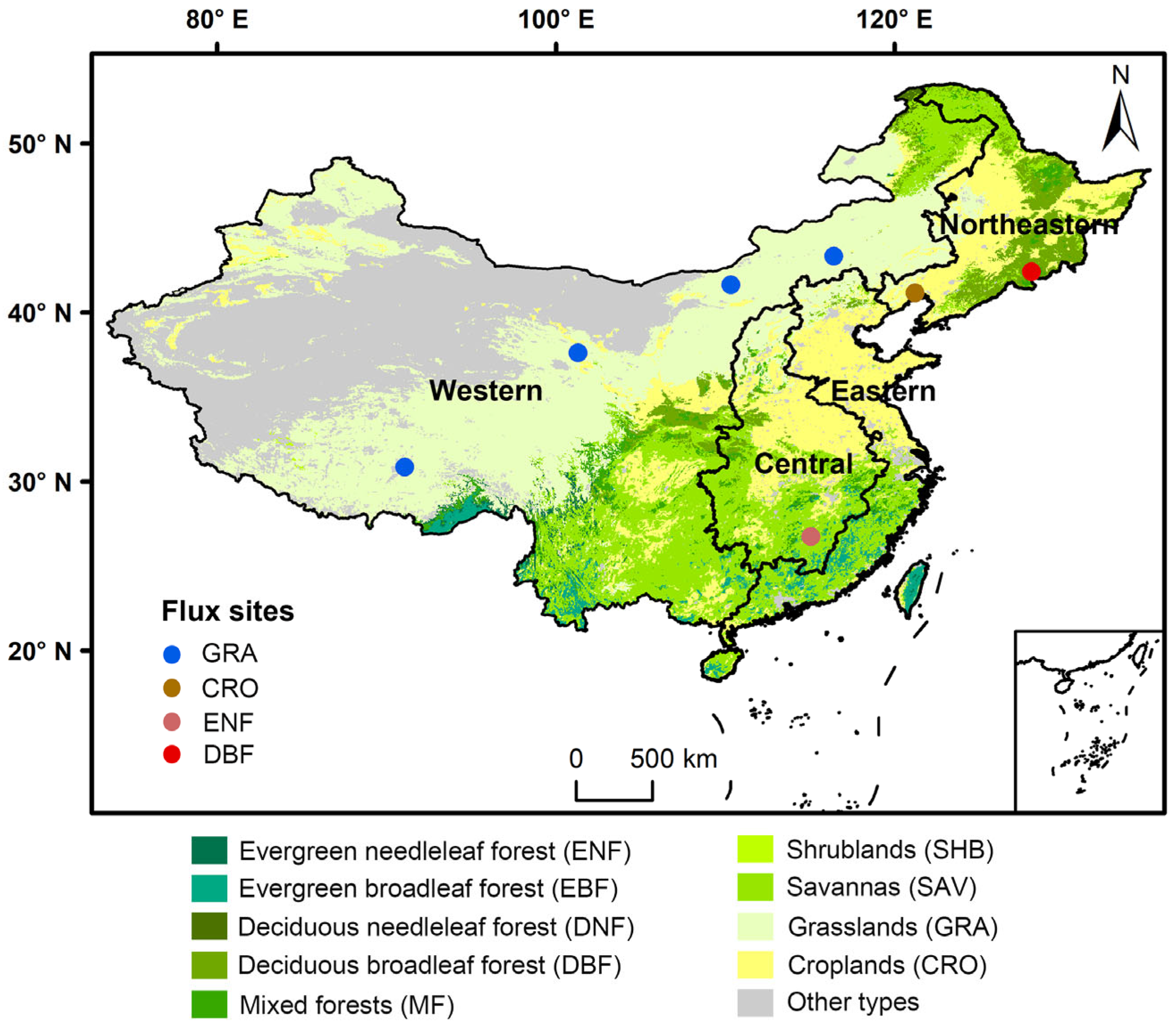
For the land cover data, the MODIS Land Cover Climate Modeling Grid (MCD12C1) Version 6 product was used. This study focused on nine major and widely distributed vegetation types in China, including evergreen needleleaf forest (ENF), evergreen broadleaf forest (EBF), deciduous needleleaf forest (DNF), deciduous broadleaf forest (DBF), mixed forests (MF), shrublands (SHB), savannas (SAV), grasslands (GRA), and croplands (CRO), with their distribution shown in Figure 1.
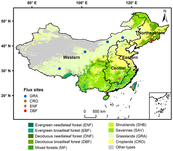
Figure 1.
Distribution of the landcover types, flux tower sites, and four economic regions across China.
We used satellite data products from 2003 to 2021 to estimate NEP and test the feasibility of the new NEP simulation framework. All satellite data were standardized to a spatial resolution of 0.05° using the arithmetic average. The spatiotemporal resolution and data acquisition details of the satellite data used in this study are shown in Table 1.

Table 1.
The spatiotemporal resolution and data accessibility details of the satellite datasets.
To test the performance of NEP simulation, we obtained 52 site-year NEP flux records across 7 flux tower sites in China (Figure 1), downloaded from the National Science & Technology Infrastructure platform (https://www.nesdc.org.cn/ (accessed on 29 January 2025)). Finally, to evaluate the synergistic variation trend between fossil fuel carbon emissions and ecosystem carbon sequestration, we obtained apparent carbon emission data for China’s four economic regions (eastern, central, western, and northeastern) from 2003 to 2021 from the Carbon Emission Accounts and Datasets (CEADs) [20,21].
2.2. Methods
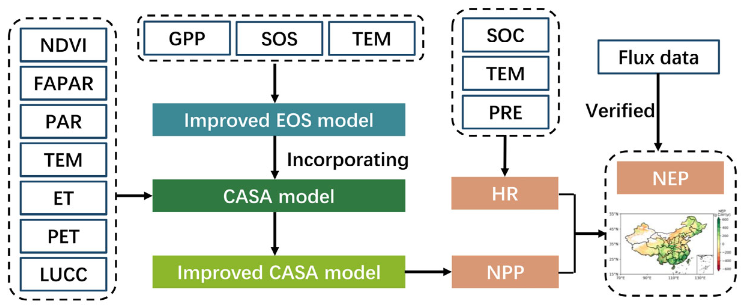
The framework for NEP improvement involved three steps: (1) improving the EOS simulation by introducing developmental factors (growing-season GPP and SOS) into the traditional autumn phenology model; (2) incorporating the improved EOS simulation into the CASA model to enhance the accuracy of NPP estimation; and finally, (3) quantifying the terrestrial NEP by subtracting the soil heterotrophic respiration from the modified NPP. The scheme of the work is illustrated in Figure 2.
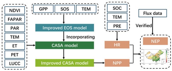
Figure 2.
The framework of NEP improvement. SOC refers to soil organic carbon density.
2.2.1. Phenological Extraction Methods
Phenology metrics were retrieved based on MODIS NDVI data. NDVI observations during the non-growing season, defined as the multiyear daily average temperature below 0 °C, were first replaced with the average value in the non-growing season. The Savitzky–Golay filter was then applied to smooth and reconstruct the NDVI curve. A double logistic function was used to fit the reconstructed NDVI time series to extract SOS and EOS. Specific details of the phenology extraction can be found in Ren et al. (2020) [22].
2.2.2. Improvement of the Autumn Phenology Model
The traditional autumn phenology model is based on low temperature accumulation, known as the cold degree day (CDD) model [10]. Considering the potential impacts of SOS and growing season GPP on EOS [9,15], we incorporated SOS, GPP, and their combination into the CDD model, naming the models CDDS, CDDG, and CDDSG, respectively. The CDD model hypothesizes that the cooling degree starts to accumulate when the daily temperature drops below the critical temperature and stops on the day of foliar senescence [10]. The formula was as follows:
where represents the accumulated cooling degree from day to day ; is the required threshold upon which EOS occurs; is the critical temperature; is the mean daily temperature on day d; and is set to 1 July [23]. The model has two free parameters, and .
For the CDDS and CDDG models, depends on SOS and the growing season GPP (Equations (3) and (4)), while the for CDDSG model is linearly linked to both SOS and the growing season GPP (Equation (5)). The of the modified models are expressed by the following equations:
where is the SOS anomaly (difference from the multiyear average SOS); is the growing season GPP anomaly (difference from the multiyear average GPP); and , , and are free parameters. To optimize free parameters in models, the simulated annealing algorithm was employed in this study. The optimal parameter combination was determined with the smallest root mean square error (RMSE) between modelled and observed EOS.
2.2.3. Modification of the CASA Model
In the CASA model, NPP was determined by the absorbed photosynthetically active radiation (APAR) and the light use efficiency () [24]. Here, APAR was obtained from the PAR and FAPAR.
where denotes the location; represents time; and is the NPP (g C/m2) at location and time .
is constrained by both temperature and moisture and is calculated as follows:
where and represent the effects of low and high temperatures on light use efficiency, respectively; is the moisture stress; and is the maximum light use efficiency under ideal conditions. Detailed calculation methods and values for , , and can be found in Liang et al. (2022) and Chen et al. (2024) [5,25].
The NPP calculated by the CASA model was interpolated to a 1-day resolution using a cubic spline function, and the CASA results were constrained by the actual vegetation phenological dates and temperature [11,26].
where is the monthly NPP simulated by the original algorithm in the CASA model, and is the result after being constrained with . is the day of year, and is daily average temperature. SOS was satellite-derived, while EOS was derived from the CDDSG model.
2.2.4. NEP Estimation
NEP was obtained by subtracting soil heterotrophic respiration (HR) from NPP.
The geostatistical model of soil respiration (GSMSR), driven by temperature, precipitation, and soil organic carbon density [27], was employed to obtain the monthly soil respiration ().
where is set as 0.588, to 0.118, to 1.83, to −0.006, to 2.972, and to 5.657 [27]. is the soil organic carbon density at 20 cm depth, varies across different vegetation types; for specific values, refer to Chen et al. (2024) [25]. and represent the monthly average temperature and precipitation, respectively.
HR was calculated based on the empirical relationship between and [5].
where is the monthly soil respiration.
2.2.5. Evaluation of Model Performances
We assessed the accuracy of the phenology model based on two metrics: RMSE and Pearson correlation coefficient (r) [10,28]. The original CASA output and the phenology-modified CASA output were compared with the MODIS gap-filled yearly NPP dataset (MOD17A3HGF) using the coefficient of determination (R2) and RMSE. Additionally, the performance of NEP estimation was also evaluated using R2 and RMSE by comparing NEP flux data with NEP data produced by either the original CASA or the phenology-modified CASA [11].
2.2.6. Analysis
We calculated the trend of terrestrial NEP across China for each pixel using the Theil-Sen trend estimator and assessed the significance of the trends at the 0.05 level with the non-parametric Mann–Kendall test [29,30]. One-way analysis of variance (ANOVA) with Tukey’s HSD test was used to examine differences in the performance of phenology models as well as differences in NEP and its trends across different vegetation types and regions. Finally, we assessed the interannual trend of the difference between fossil fuel carbon emissions and ecosystem carbon sequestration in China’s four economic regions. All analyses were performed in Python.
3. Results
3.1. Performances Assessment of Models
Overall, the models that incorporated developmental factors outperformed the original phenology model (Figure 3a,b). The CDDSG model achieved the highest average r values (0.10), significantly surpassing the other models, followed by the CDDS (0.09), CDDG (0.03), and CDD models (0.01). In terms of the prediction accuracy, the EOS simulated by the CDDG model exhibited a significantly lower RMSE (14.27 days) compared to other models, followed by CDDSG (14.95 days), CDDS (15.32 days), and CDD (18.28 days). Based on these results, we introduced the EOS predicted by the CDDSG model into the CASA model.
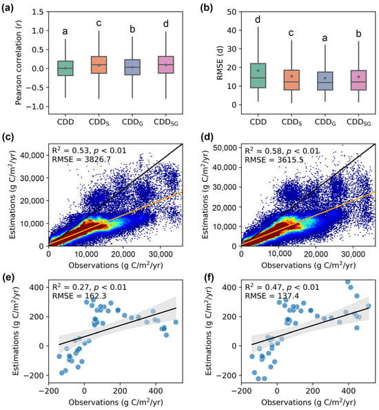
Figure 3.
Model performance comparison. (a,b) Pearson’s correlation coefficient and RMSE between predicted EOS from different phenology models and observed EOS, respectively. Different letters indicate significant differences among models (p < 0.05). (c,d) Comparison between the NPP modeled by the original CASA and the phenology-modified CASA with MODIS NPP, respectively. (e,f) Accuracy of NEP produced by the original CASA and the phenology-modified CASA compared to the NEP flux observations, respectively.
The NPP produced by the phenology-modified CASA model was more consistent with the MODIS NPP (Figure 3c,d). Specifically, the NPP simulated by the phenology-modified CASA model displayed a relatively higher R2 (0.58 vs. 0.53) and lower RMSE (3615.5 vs. 3826.7 g C/m2/yr) compared to the counterparts of the original CASA model. Similarly, the following comparison of NEP based on the original CASA model and the phenology-modified CASA model against flux tower NEP observations revealed that the RMSE of the phenology-modified model decreased by 15.34% compared to the original model, while the R2 increased from 0.27 to 0.47, representing an improvement of approximately 74% (Figure 3e,f).
3.2. Spatial Patterns of NEP Estimates
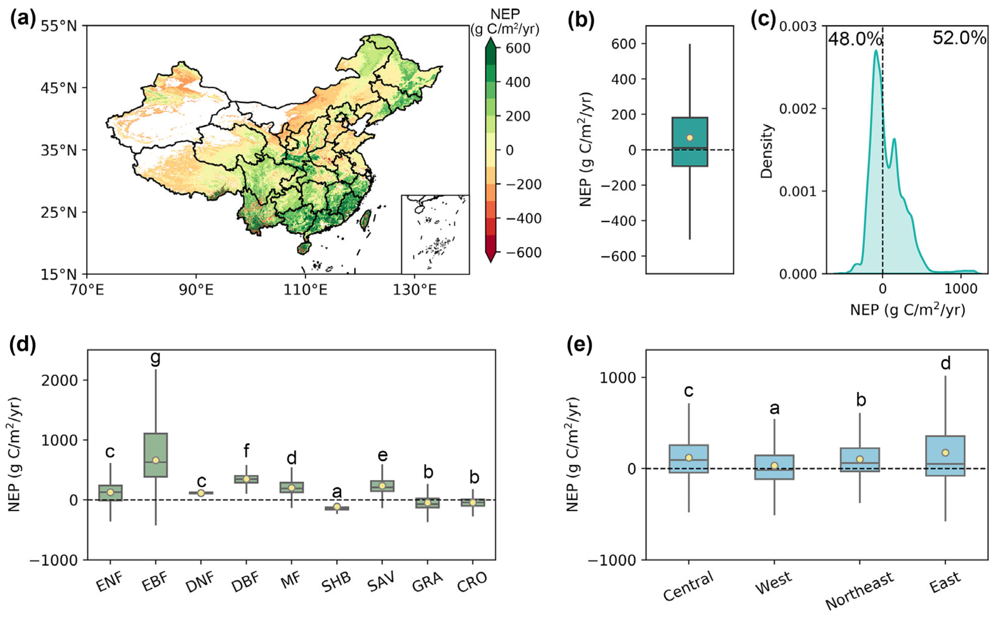
From 2003 to 2021, the total annual average NEP over China was 489.67 ± 38.27 Tg C/yr (mean ± standard error), with an average of 68.78 g C/m2/yr per unit area (Figure 4a,b). Of the pixels, 52.0% showed a multiyear average NEP greater than 0, serving as carbon sinks (Figure 4c). Spatially, stronger carbon sink capabilities were observed in the southeast, southwest, and the three northeastern provinces, generally exceeding 300 g C/m2/yr, while most of the Bohai Sea Rim area, Inner Mongolia, and the central region of the Qinghai–Tibet Plateau exhibited weak carbon sources (Figure 4a).
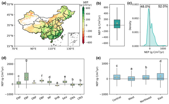
Figure 4.
The multiyear mean of annual NEP in China produced by the phenology-modified CASA model during 2003–2021. (a) The spatial pattern of the multiyear mean NEP during 2003–2021. (b) The multiyear mean NEP over China. (c) The density distribution of the multiyear mean annual NEP. (d,e) Multiyear mean NEP across various vegetation types and economic regions. The yellow dots represent the mean value, and the horizontal lines within the bars denote the median value. Different letters indicate significant differences among models (p < 0.05).
Across diverse vegetation types, the multiyear average NEP of EBF (600.53 g C/m2/yr) was significantly higher than that of other vegetation types, followed by DBF (348.64 g C/m2/yr) and SAV (236.48 g C/m2/yr) (Figure 4d). In contrast, SHB, GRA, and CRO functioned as carbon sources, displaying negative multiyear average NEP values of −113.34, −46.16, and −45.43 g C/m2/yr, respectively. From a regional perspective, all four economic regions in China played a role as carbon sinks from 2003 to 2021 (Figure 4e). The multiyear average NEP in the eastern region (174.17 g C/m2/yr) was the greatest, likely due to the highest forest coverage in China, followed by the northeastern, central, and western regions, with NEP values of 119.52, 101.59, and 32.49 g C/m2/yr, respectively.
3.3. Temporal Trends of NEP Estimates
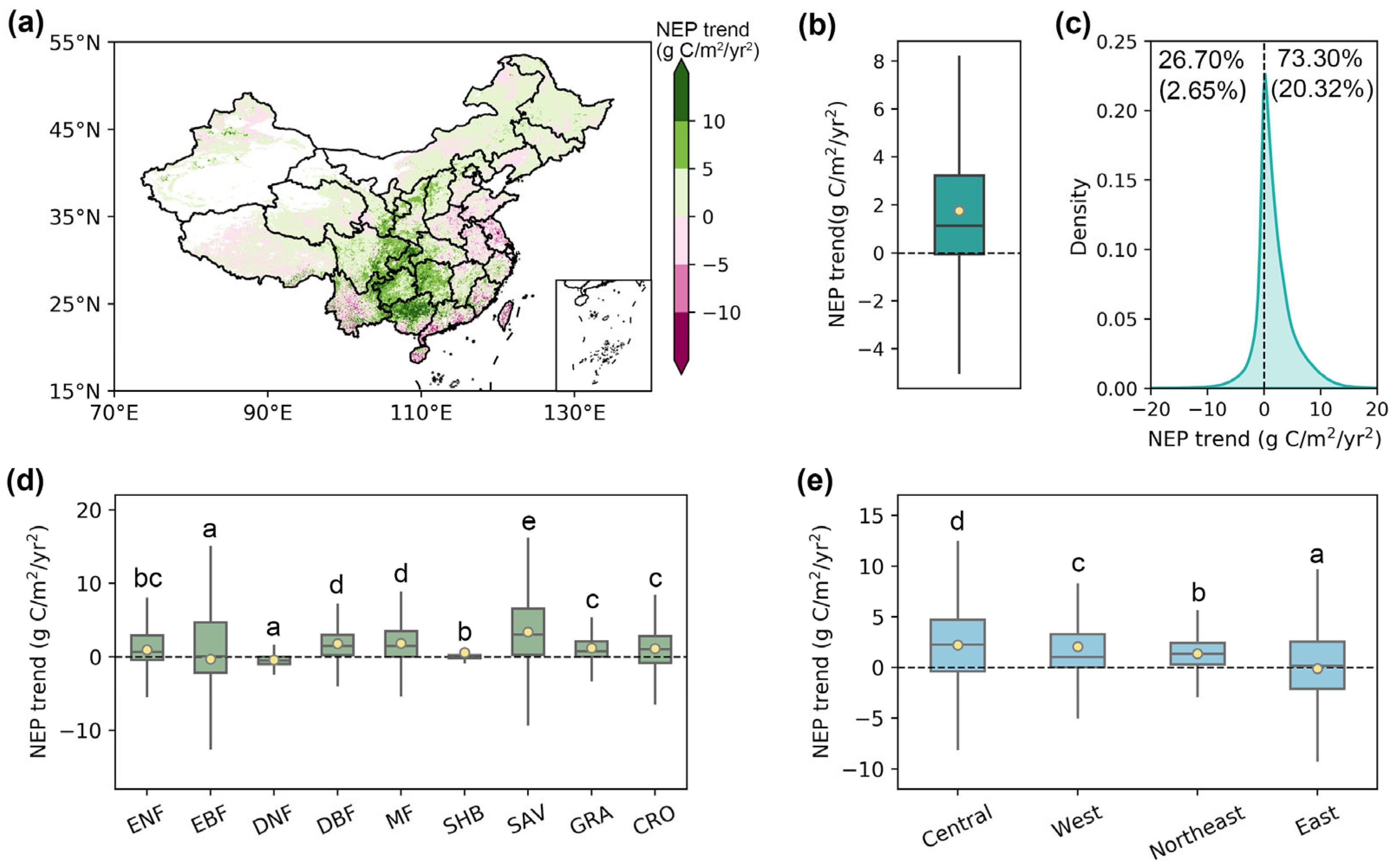
Overall, this study found an increasing tendency of NEP in China with an average rate of 1.75 g C/m2/yr2 from 2003 to 2021 (Figure 5a,b). Specifically, this increasing trend was identified in 73.30% of the pixels, with 20.32% passing the significance test (Figure 5c). Spatially, the increase in NEP was primarily concentrated in central regions, such as Guizhou, Chongqing, and Hunan, while most eastern coastal areas exhibited a declining trend. Further investigation revealed an increment of NEP across all vegetation types except for EBF and DNF. Among them, SAV exhibited the highest NEP growth rate of 3.40 g C/m2/yr2, followed by MF (1.83 g C/m2/yr2) and DBF (1.81 g C/m2/yr2). Subregionally, all areas showed positive NEP trends during the study period, except the economically developed eastern region (−0.01 g C/m2/yr2), with the central region exhibiting the most pronounced increase at 2.21 g C/m2/yr2.
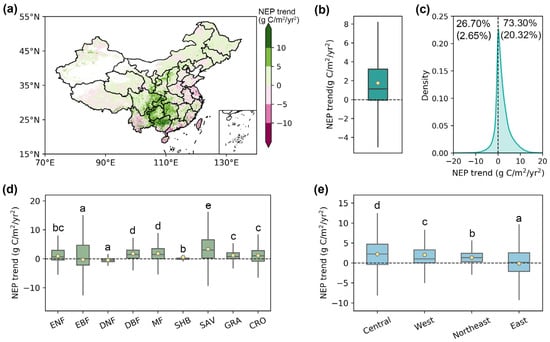
Figure 5.
The trends of NEP in China produced by the phenology-modified CASA model during 2003–2021. (a) The spatial pattern of NEP trend from 2003 to 2021. (b) The mean NEP trend across China. (c) The density distribution of the NEP trend. The numbers in parentheses represent the proportion that passed the significance test (p < 0.05). (d,e) The NEP trend across different vegetation types and economic regions. The yellow dots represent the mean value, and the horizontal lines within the bars denote the median value. Different letters indicate significant differences among models (p < 0.05).
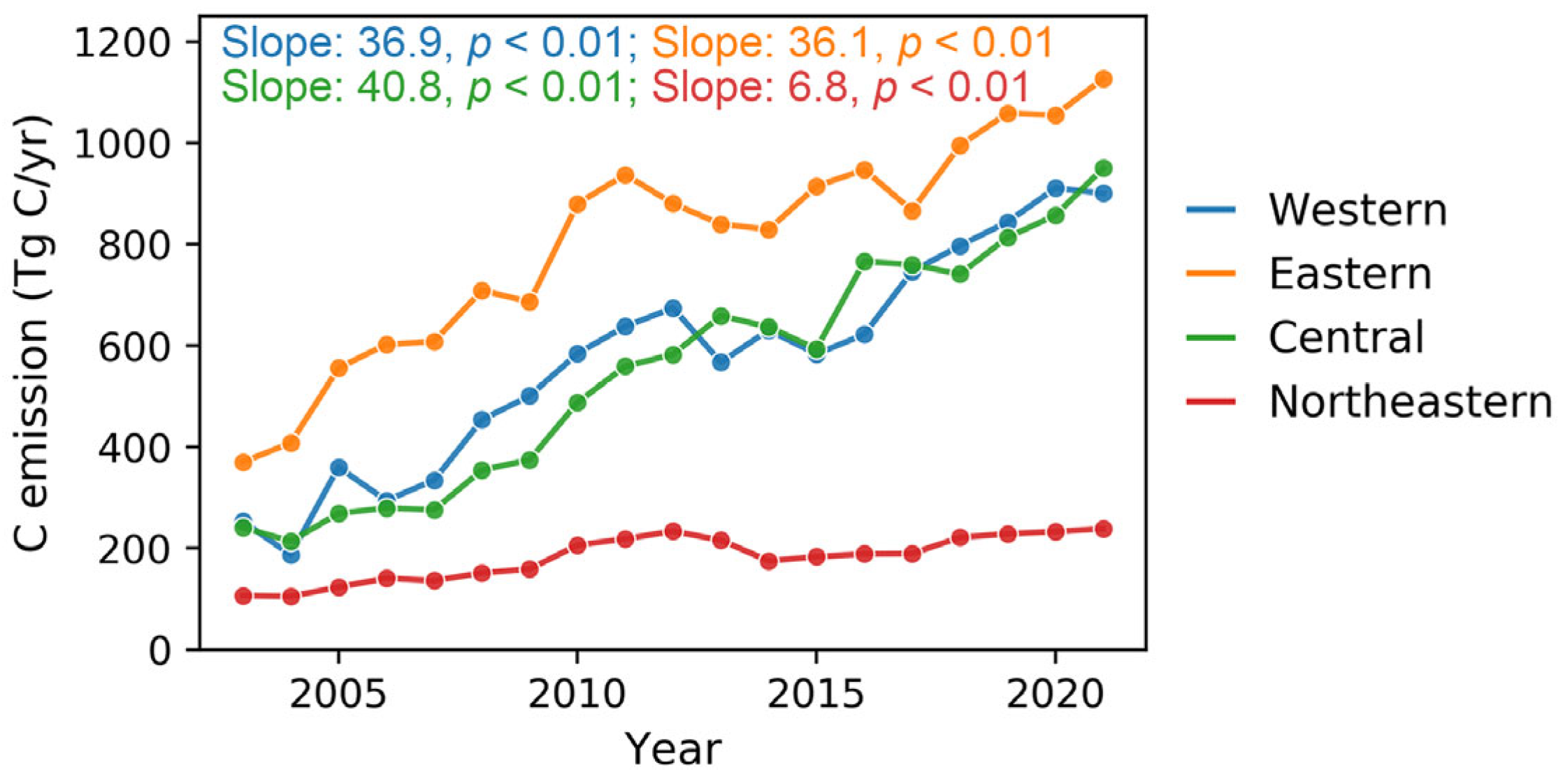
By analyzing the trends in the difference between total apparent carbon emissions and ecosystem NEP, we identified significant regional disparities in carbon neutrality progress across China’s regions (Figure 6). The central region exhibited the fastest net carbon emission growth, reaching 40.8 Tg C/yr, suggesting that carbon emissions from fossil fuel consumption substantially outpaced the enhancement in ecosystem carbon sequestration. The western and eastern regions showed comparable net carbon emission growth rates of 36.9 and 36.1 Tg C/yr, respectively. In contrast, the northeastern region performed the most favorably, exhibiting both the lowest total net carbon emissions throughout the study period and the most modest growth rate at 6.8 Tg C/yr.

Figure 6.
The tendency comparison of the difference between apparent carbon emissions and terrestrial NEP in China’s four economic regions from 2003 to 2021.
4. Discussion
Accurate phenological models are crucial tools for predicting vegetation phenological responses to future climate scenarios and their subsequent impacts on ecosystem functions [31,32]. Given the significant influence of developmental factors on autumn phenology, this study enhanced the traditional autumn phenology model by incorporating growing season GPP and SOS. The results showed that whether considering GPP or SOS alone or incorporating both factors, the modified autumn phenology models outperformed the original temperature-based model, significantly enhancing the simulation capability of autumn phenology (Figure 3). Traditional temperature-based models predict that under future warming conditions, vegetation productivity will increase due to extended growing seasons [8,33]. However, in temperate forests of the Northern Hemisphere, increased growing season productivity and earlier spring phenology triggered by rising CO2 concentrations, higher temperatures, or changes in light levels may accelerate plant senescence, potentially offsetting the promotional effects of warming on growing season extension [9,15]. Therefore, current phenological models that do not consider developmental factors may seriously overestimate future growing season length, leading to significant biases in global carbon cycle estimates [8,9]. Future research should fully integrate developmental factors into predictions of plant phenology, which may revise our expectations of plant carbon sequestration capacity and avoid overly optimistic estimates of ecosystem carbon sink potential under future climate change.
In recent years, numerous studies have employed various methods to estimate the carbon sink capacity of China’s terrestrial ecosystems [4,5,25]. While estimates vary across methodologies, there is consensus that China’s terrestrial ecosystems act as a significant carbon sink [2,3]. Piao et al. (2022) [3] systematically compared estimates from different periods and methods, revealing that China’s terrestrial ecosystems exhibit a carbon sink capacity ranging from 0.12 to 1.11 Pg C/yr. Our study estimated an average NEP of 0.49 Pg C/yr for the period 2003–2021, which falls within the credible range but is slightly higher than estimates from ecosystem process models. This discrepancy likely stems from variations in temporal coverage, as China’s NEP has shown significant increases since the 21st century [34], while other studies include NEP data from before 2000, lowering the overall average in those estimates. On the other hand, the spatial distribution of NEP estimated in our study aligns with previous studies [2,4,25], with strong carbon sink areas primarily located in the southeastern and southwestern parts of China. Forests serve as the primary carbon sinks, while shrubs, grasslands, and croplands act as weak carbon sources (Figure 4). Forest ecosystems have high productivity and carbon storage capacity, and studies have shown that existing global forests alone can account for the land carbon sink [35]. In contrast, shrubs and grasslands have low biomass and limited carbon storage capacity, with carbon absorption and respiration being generally balanced, resulting in a weak carbon sink or even a carbon source [36,37].
Consistent with other studies, China’s terrestrial carbon sink showed a significant upward trend from 2003 to 2021 (Figure 5), likely driven by multiple factors. First, the fertilization effect of increased atmospheric CO2 concentrations significantly enhanced plant photosynthesis efficiency, thereby promoting carbon uptake [17,38]. Second, in both the northern and southern forest regions, climate warming extended the growing season, which may have further strengthened carbon sequestration capacity [8]. Additionally, in southeastern China, increased anthropogenic nitrogen deposition has been shown to have a significant positive impact on plant growth [39], potentially providing crucial support for the enhancement of carbon sinks [40]. Finally, human interventions played a key role, such as large-scale afforestation projects contributing to over 70% of forest area expansion, natural forest protection, and ecological restoration programs, like the conversion of grazing land to grassland, which effectively promoted vegetation growth and enhanced ecosystem carbon sequestration capacity [41,42]. The combined effects of CO2 fertilization, climate warming, increased nitrogen deposition, and human interventions collectively drove the continuous growth of China’s terrestrial carbon sink.
Our analysis of the residual emissions after offsetting industrial carbon emissions with the carbon sink of China’s terrestrial ecosystems revealed that, across all economic regions, the growth in ecosystem carbon sinks was smaller than the increase in carbon emissions from fossil fuel combustion during the same period (Figure 6). There were also regional differences in carbon neutrality levels. The economically developed eastern regions, including the Bohai Sea Rim and the Huang–Huai–Hai region, were far from achieving carbon neutrality. These areas were predominantly cropland with inherently weak carbon sink capacity, combined with high levels of industrial development and dense populations, leading to significantly higher apparent carbon emissions and residual emissions compared to other regions. In contrast, the northeastern region, with its relatively slower economic growth, showed a slower increase in residual emissions and exhibited better carbon neutrality levels than other regions. The western and central regions had relatively similar levels of carbon neutrality. Studies have suggested that as China’s forests gradually mature and age, the carbon sink capacity might decline, further reducing the ability of terrestrial ecosystems to offset industrial carbon emissions [3,43]. Therefore, achieving carbon neutrality requires the coordinated implementation of multiple strategies.
The NEP simulation framework we developed also has some uncertainties. First, discrepancies may exist between the actual start and end dates of plant photosynthesis and the SOS and EOS derived from the phenology model. Studies have shown that photosynthesis can continue until chlorophyll depletion in the leaves [44]. Second, ecosystem process models, such as CASA, do not account for human factors, like irrigation, fertilization, and forest management, all of which can significantly influence plant growth [3]. This adds uncertainty to the NEP estimates, and caution is needed when applying these models to agricultural ecosystems. Furthermore, ecosystem process models rely on remote sensing data, and the accuracy of these estimates is highly dependent on the quality of the remote sensing data [11]. The relatively coarse resolution of remote sensing data may also obscure NEP variations in specific plant types [22]. In the future, when extending our NEP accounting framework to larger study areas, special attention should be given to data quality, and multi-source data should be used for cross-validation to improve the reliability of the estimates. Additionally, more factors influencing plant growth should be incorporated into carbon sink accounting models to improve their comprehensiveness and accuracy.
5. Conclusions
This study enhanced NEP estimation by incorporating developmental factors (growing-season GPP and SOS) into autumn phenology model and using the modified phenology outputs to constrain the CASA model. The integration of developmental factors significantly improved the autumn phenology model’s performance, resulting in lower RMSE and higher correlation. The CASA model, constrained by phenological information, exhibited markedly better alignment with MODIS NPP products. Moreover, compared to the original model, the NEP produced by the phenology-modified CASA model achieved a 15.34% reduction in RMSE and a 74% improvement in R2 against flux tower observations. From 2003 to 2021, the annual average total NEP of China’s terrestrial ecosystems was 489.67 ± 38.27 Tg C/yr and significantly increased with an average growth rate of 1.75 g C/m2/yr2. Among vegetation types, evergreen broadleaf forests maintained the highest NEP, while shrublands exhibited the lowest values. However, the NEP growth rates across all four economic regions remained insufficient to offset the concurrent increases in industrial carbon emissions, with eastern China showing the highest net carbon emissions and facing significant challenges in achieving carbon neutrality. This study proposes a new and more accurate framework for NEP estimation, which provides valuable insights for understanding and predicting China’s carbon sink strength and offers scientific support for the formulation of carbon neutrality policies.
Supplementary Materials
The following supporting information can be downloaded at: https://www.mdpi.com/article/10.3390/rs17030487/s1, Figure S1: Correlation of interannual fluctuations between different GPP datasets.
Author Contributions
Conceptualization, S.J. and S.R.; methodology, S.J. and S.R.; investigation, S.J.; writing—original draft preparation, S.J. and S.R.; writing—review and editing, L.F., J.C., G.W., and Q.W. All authors have read and agreed to the published version of the manuscript.
Funding
This study is supported by the National Key R&D Program of China (No. 2022YFC3204400) and the National Natural Science Foundation of China Key Program (No. 52339002).
Data Availability Statement
All data used in this study could be obtained freely online.
Acknowledgments
We acknowledge the data support from National Earth System Science Data Center, National Science & Technology Infrastructure of China.
Conflicts of Interest
The authors declare no conflicts of interest.
References
- Le Quéré, C.; Moriarty, R.; Andrew, R.M.; Canadell, J.G.; Sitch, S.; Korsbakken, J.I.; Friedlingstein, P.; Peters, G.P.; Andres, R.J.; Boden, T.A.; et al. Global Carbon Budget 2015. Earth Syst. Sci. Data 2015, 7, 349–396. [Google Scholar] [CrossRef]
- Jung, M.; Reichstein, M.; Margolis, H.A.; Cescatti, A.; Richardson, A.D.; Arain, M.A.; Arneth, A.; Bernhofer, C.; Bonal, D.; Chen, J.; et al. Global patterns of land-atmosphere fluxes of carbon dioxide, latent heat, and sensible heat derived from eddy covariance, satellite, and meteorological observations. J. Geophys. Res. Biogeosci. 2011, 116, G00J07. [Google Scholar] [CrossRef]
- Piao, S.; He, Y.; Wang, X.; Chen, F. Estimation of China’s terrestrial ecosystem carbon sink: Methods, progress and prospects. Sci. China Earth Sci. 2022, 65, 641–651. [Google Scholar] [CrossRef]
- Yao, Y.; Li, Z.; Wang, T.; Chen, A.; Wang, X.; Du, M.; Jia, G.; Li, Y.; Li, H.; Luo, W.; et al. A new estimation of China’s net ecosystem productivity based on eddy covariance measurements and a model tree ensemble approach. Agric. For. Meteorol. 2018, 253–254, 84–93. [Google Scholar] [CrossRef]
- Liang, L.; Geng, D.; Yan, J.; Qiu, S.; Shi, Y.; Wang, S.; Wang, L.; Zhang, L.; Kang, J. Remote Sensing Estimation and Spatiotemporal Pattern Analysis of Terrestrial Net Ecosystem Productivity in China. Remote Sens. 2022, 14, 1902. [Google Scholar] [CrossRef]
- Friedlingstein, P.; O’Sullivan, M.; Jones, M.W.; Andrew, R.M.; Bakker, D.C.E.; Hauck, J.; Landschützer, P.; Le Quéré, C.; Luijkx, I.T.; Peters, G.P.; et al. Global Carbon Budget 2023. Earth Syst. Sci. Data 2023, 15, 5301–5369. [Google Scholar] [CrossRef]
- Piao, S.; Liu, Z.; Wang, T.; Peng, S.; Ciais, P.; Huang, M.; Ahlstrom, A.; Burkhart, J.F.; Chevallier, F.; Janssens, I.A.; et al. Weakening temperature control on the interannual variations of spring carbon uptake across northern lands. Nat. Clim. Chang. 2017, 7, 359–363. [Google Scholar] [CrossRef]
- Keenan, T.F.; Gray, J.; Friedl, M.A.; Toomey, M.; Bohrer, G.; Hollinger, D.Y.; Munger, J.W.; O’Keefe, J.; Schmid, H.P.; Wing, I.S.; et al. Net carbon uptake has increased through warming-induced changes in temperate forest phenology. Nat. Clim. Chang. 2014, 4, 598–604. [Google Scholar] [CrossRef]
- Zani, D.; Crowther, T.W.; Mo, L.; Renner, S.S.; Zohner, C.M. Increased growing-season productivity drives earlier autumn leaf senescence in temperate trees. Science 2020, 370, 1066–1071. [Google Scholar] [CrossRef]
- Keenan, T.F.; Richardson, A.D. The timing of autumn senescence is affected by the timing of spring phenology: Implications for predictive models. Glob. Change Biol. 2015, 21, 2634–2641. [Google Scholar] [CrossRef]
- Peng, J.; Wu, C.; Zhang, X.; Ju, W.; Wang, X.; Lu, L.; Liu, Y. Incorporating water availability into autumn phenological model improved China’s terrestrial gross primary productivity (GPP) simulation. Environ. Res. Lett. 2021, 16, 094012. [Google Scholar] [CrossRef]
- Zohner, C.M.; Mirzagholi, L.; Renner, S.S.; Mo, L.; Rebindaine, D.; Bucher, R.; Palouš, D.; Vitasse, Y.; Fu, Y.H.; Stocker, B.D.; et al. Effect of climate warming on the timing of autumn leaf senescence reverses after the summer solstice. Science 2023, 381, eadf5098. [Google Scholar] [CrossRef] [PubMed]
- Buermann, W.; Bikash, P.R.; Jung, M.; Burn, D.H.; Reichstein, M. Earlier springs decrease peak summer productivity in North American boreal forests. Environ. Res. Lett. 2013, 8, 024027. [Google Scholar] [CrossRef]
- Lam, E. Controlled cell death, plant survival and development. Nat. Rev. Mol. Cell Biol. 2004, 5, 305–315. [Google Scholar] [CrossRef]
- Fu, Y.S.H.; Campioli, M.; Vitasse, Y.; De Boeck, H.J.; Van den Berge, J.; AbdElgawad, H.; Asard, H.; Piao, S.; Deckmyn, G.; Janssens, I.A. Variation in leaf flushing date influences autumnal senescence and next year’s flushing date in two temperate tree species. Proc. Natl. Acad. Sci. USA 2014, 111, 7355–7360. [Google Scholar] [CrossRef]
- Zheng, Y.; Shen, R.; Wang, Y.; Li, X.; Liu, S.; Liang, S.; Chen, J.M.; Ju, W.; Zhang, L.; Yuan, W. Improved estimate of global gross primary production for reproducing its long-term variation, 1982–2017. Earth Syst. Sci. Data 2020, 12, 2725–2746. [Google Scholar]
- Wang, S.; Zhang, Y.; Ju, W.; Chen, J.M.; Ciais, P.; Cescatti, A.; Sardans, J.; Janssens, I.A.; Wu, M.; Berry, J.A.; et al. Recent global decline of CO2 fertilization effects on vegetation photosynthesis. Science 2020, 370, 1295–1300. [Google Scholar] [CrossRef]
- Peng, S.; Ding, Y.; Liu, W.; Li, Z. 1 km monthly temperature and precipitation dataset for China from 1901 to 2017. Earth Syst. Sci. Data 2019, 11, 1931–1946. [Google Scholar] [CrossRef]
- Peng, S.; Ding, Y.; Wen, Z.; Chen, Y.; Cao, Y.; Ren, J. Spatiotemporal change and trend analysis of potential evapotranspiration over the Loess Plateau of China during 2011–2100. Agric. For. Meteorol. 2017, 233, 183–194. [Google Scholar] [CrossRef]
- Guan, Y.; Shan, Y.; Huang, Q.; Chen, H.; Wang, D.; Hubacek, K. Assessment to China’s Recent Emission Pattern Shifts. Earth’s Future 2021, 9, e2021EF002241. [Google Scholar] [CrossRef]
- Shan, Y.; Huang, Q.; Guan, D.; Hubacek, K. China CO2 emission accounts 2016–2017. Sci. Data 2020, 7, 54. [Google Scholar] [CrossRef] [PubMed]
- Ren, S.; Li, Y.; Peichl, M. Diverse effects of climate at different times on grassland phenology in mid-latitude of the Northern Hemisphere. Ecol. Indic. 2020, 113, 106260. [Google Scholar] [CrossRef]
- Wu, C.; Wang, J.; Ciais, P.; Peñuelas, J.; Zhang, X.; Sonnentag, O.; Tian, F.; Wang, X.; Wang, H.; Liu, R.; et al. Widespread decline in winds delayed autumn foliar senescence over high latitudes. Proc. Natl. Acad. Sci. USA 2021, 118, e2015821118. [Google Scholar] [CrossRef] [PubMed]
- Potter, C.S.; Randerson, J.T.; Field, C.B.; Matson, P.A.; Vitousek, P.M.; Mooney, H.A.; Klooster, S.A. Terrestrial ecosystem production: A process model based on global satellite and surface data. Glob. Biogeochem. Cycles 1993, 7, 811–841. [Google Scholar] [CrossRef]
- Chen, Y.; Xu, Y.; Chen, T.; Zhang, F.; Zhu, S. Exploring the Spatiotemporal Dynamics and Driving Factors of Net Ecosystem Productivity in China from 1982 to 2020. Remote Sens. 2024, 16, 60. [Google Scholar] [CrossRef]
- Gonsamo, A.; Chen, J.M.; Price, D.T.; Kurz, W.A.; Liu, J.; Boisvenue, C.; Hember, R.A.; Wu, C.; Chang, K.-H. Improved assessment of gross and net primary productivity of Canada’s landmass. J. Geophys. Res. Biogeosci. 2013, 118, 1546–1560. [Google Scholar] [CrossRef]
- Yu, G.; Zheng, Z.; Wang, Q.; Fu, Y.; Zhuang, J.; Sun, X.; Wang, Y. Spatiotemporal Pattern of Soil Respiration of Terrestrial Ecosystems in China: The Development of a Geostatistical Model and Its Simulation. Environ. Sci. Technol. 2010, 44, 6074–6080. [Google Scholar] [CrossRef]
- Wu, C.; Peng, J.; Ciais, P.; Peñuelas, J.; Wang, H.; Beguería, S.; Andrew Black, T.; Jassal, R.S.; Zhang, X.; Yuan, W.; et al. Increased drought effects on the phenology of autumn leaf senescence. Nat. Clim. Chang. 2022, 12, 943–949. [Google Scholar] [CrossRef]
- Mann, H.B. Nonparametric Tests Against Trend. Econometrica 1945, 13, 245–259. [Google Scholar] [CrossRef]
- Kendall, M.G. Rank Correlation Methods; Griffin: Oxford, UK, 1948. [Google Scholar]
- Fu, Y.; Li, X.; Zhou, X.; Geng, X.; Guo, Y.; Zhang, Y. Progress in plant phenology modeling under global climate change. Sci. China Earth Sci. 2020, 63, 1237–1247. [Google Scholar] [CrossRef]
- Piao, S.; Liu, Q.; Chen, A.; Janssens, I.A.; Fu, Y.; Dai, J.; Liu, L.; Lian, X.; Shen, M.; Zhu, X. Plant phenology and global climate change: Current progresses and challenges. Glob. Change Biol. 2019, 25, 1922–1940. [Google Scholar] [CrossRef] [PubMed]
- Menzel, A.; Fabian, P. Growing season extended in Europe. Nature 1999, 397, 659. [Google Scholar] [CrossRef]
- Shi, Y.; Yang, C.; Zhu, J.; Chang, J.; Zhao, X.; Sun, W.; Huang, M.; Yu, Y.; Guo, K.; Gu, F.; et al. Estimation of national and provincial carbon emissions, terrestrial carbon sinks and their relative contribution to emission reductions during 1980~2020. Sci. Sin. Vitae 2024, 54, 2459–2478. [Google Scholar] [CrossRef]
- Pan, Y.; Birdsey, R.A.; Fang, J.; Houghton, R.; Kauppi, P.E.; Kurz, W.A.; Phillips, O.L.; Shvidenko, A.; Lewis, S.L.; Canadell, J.G.; et al. A Large and Persistent Carbon Sink in the World’s Forests. Science 2011, 333, 988–993. [Google Scholar] [CrossRef]
- Lal, R. Soil Carbon Sequestration Impacts on Global Climate Change and Food Security. Science 2004, 304, 1623–1627. [Google Scholar] [CrossRef]
- Schlesinger, W.H.; Andrews, J.A. Soil respiration and the global carbon cycle. Biogeochemistry 2000, 48, 7–20. [Google Scholar] [CrossRef]
- Fang, J.; Kato, T.; Guo, Z.; Yang, Y.; Hu, H.; Shen, H.; Zhao, X.; Kishimoto-Mo, A.W.; Tang, Y.; Houghton, R.A. Evidence for environmentally enhanced forest growth. Proc. Natl. Acad. Sci. USA 2014, 111, 9527–9532. [Google Scholar] [CrossRef]
- Liu, X.; Zhang, Y.; Han, W.; Tang, A.; Shen, J.; Cui, Z.; Vitousek, P.; Erisman, J.W.; Goulding, K.; Christie, P.; et al. Enhanced nitrogen deposition over China. Nature 2013, 494, 459–462. [Google Scholar] [CrossRef]
- Piao, S.; Yin, G.; Tan, J.; Cheng, L.; Huang, M.; Li, Y.; Liu, R.; Mao, J.; Myneni, R.B.; Peng, S.; et al. Detection and attribution of vegetation greening trend in China over the last 30 years. Glob. Change Biol. 2015, 21, 1601–1609. [Google Scholar] [CrossRef]
- Lu, F.; Hu, H.; Sun, W.; Zhu, J.; Liu, G.; Zhou, W.; Zhang, Q.; Shi, P.; Liu, X.; Wu, X.; et al. Effects of national ecological restoration projects on carbon sequestration in China from 2001 to 2010. Proc. Natl. Acad. Sci. USA 2018, 115, 4039–4044. [Google Scholar] [CrossRef]
- Yang, C.; Shi, Y.; Sun, W.; Zhu, J.; Ji, C.; Feng, Y.; Ma, S.; Guo, Z.; Fang, J. Updated estimation of forest biomass carbon pools in China, 1977–2018. Biogeosciences 2022, 19, 2989–2999. [Google Scholar] [CrossRef]
- Leng, Y.; Li, W.; Ciais, P.; Sun, M.; Zhu, L.; Yue, C.; Chang, J.; Yao, Y.; Zhang, Y.; Zhou, J.; et al. Forest aging limits future carbon sink in China. One Earth 2024, 7, 822–834. [Google Scholar] [CrossRef]
- Keskitalo, J.; Bergquist, G.; Gardeström, P.; Jansson, S. A Cellular Timetable of Autumn Senescence. Plant Physiol. 2005, 139, 1635–1648. [Google Scholar] [CrossRef] [PubMed]

Disclaimer/Publisher’s Note: The statements, opinions and data contained in all publications are solely those of the individual author(s) and contributor(s) and not of MDPI and/or the editor(s). MDPI and/or the editor(s) disclaim responsibility for any injury to people or property resulting from any ideas, methods, instructions or products referred to in the content. |
© 2025 by the authors. Licensee MDPI, Basel, Switzerland. This article is an open access article distributed under the terms and conditions of the Creative Commons Attribution (CC BY) license (https://creativecommons.org/licenses/by/4.0/).