Abstract
The growth of photovoltaic (PV) installations is essential for the global energy transition; however, comprehensive data regarding their spatial distribution are limited, which complicates effective energy planning. This research introduces a methodology for automatic recognition of ground-mounted PV systems in Italy, using semantic segmentation and Sentinel-2 RGB images with a resolution of 10 m. The objective of this methodology is to accurately identify both the locations and the sizes of these installations, estimate their capacity, and facilitate regular updates to maps, thereby supporting energy planning strategies. The segmentation model, which is founded on a U-Net architecture, is trained using a dataset from 2019 and evaluated on two separate cases that involve different dates and geographical areas. We propose a multi-temporal approach, applying the model to a sequence of images taken throughout the year and aggregating the results to create a PV detection probability map. Users have the flexibility to modify probability thresholds to enhance accuracy: lower thresholds increase producer accuracy, ensuring continuous area detection for capacity estimation, while higher thresholds boost user accuracy by reducing false positives. Additionally, post-processing techniques, such as filtering for plastic-covered greenhouses, assist minimizing detection errors. However, there is a need for improved model generalizability across various landscapes, necessitating retraining with images from a range of environmental contexts.
1. Introduction
In recent years, to achieve decarbonization goals, there has been a significant increase in photovoltaic (PV) installations, representing a key renewable energy source for the energy transition [1,2]. For optimized energy planning, territorial characterization is crucial, including knowing the locations of currently installed PV ground-mounted systems. Despite the growing interest in this technology, both in Italy and globally, there is a lack of available data regarding the distribution of PV installations across the territory. When such data are accessible, they are frequently outdated, rendering them less effective in a rapidly changing environment [3]. While operators are aware of the locations and capacities of these installations, there is often an absence of publicly accessible data that would facilitate analysis of the spatial distribution of existing installations and their development over time.
The most recent attempts to map renewable energy systems (RES) on a national or continental scale are based on data derived from crowdsourcing initiatives (e.g., OpenStreetMap), existing harmonized databases, or measurement campaigns [4,5,6]. While these initiatives are extremely useful, especially for humanitarian purposes, they rely on communities of volunteers who contribute to the maintenance and updating of the mapped information [7]. As a result, the coverage, accuracy, and currency of the mapped data are not uniform, depending heavily on the efforts of each community, and need to be verified and validated by expert users [8].
Remote sensing (RS) is a non-invasive surveying technique for studying and monitoring of the Earth’s surface through long-distance observation and has been effectively used in the past to address various needs related to the development of PV systems [9]. In the literature, several examples can be found where RS data were applied to estimate the PV potential of a territory [10,11,12], to detect and monitor failures in PV systems [13,14], as well as to map ground-mounted or rooftop PV installations [15,16,17]. Thanks to the spatial coverage of the data, the update frequency, the availability of multiple types of free acquisitions, and the wide range of data processing techniques and algorithms, satellite or aerial RS can be successfully applied for the identification of PV installations for energy planning purposes. This constitutes an alternative to the aforementioned methods based on data collection from existing databases, field surveys, or crowdsourcing campaigns [18].
From the earliest studies on the subject [19,20], two main methods for PV systems mapping were identified: (1) physically based approaches, using hyperspectral images; and (2) the application of machine learning (ML) algorithms to multispectral images. Physically based approaches exploit the reflectance characteristics of PV panels across different bands of the electromagnetic spectrum to extract installations from the surrounding background. The layered composition of PV modules generates a spectral signature characterized by low reflectance values in the visible wavelengths (i.e., between 400 nm and 700 nm), a rapid increase in reflectance between 900 nm and 1150 nm, and two strong absorption dips around 1730 nm and 2200 nm [20]. However, these details can only be detected through hyperspectral remote sensing, including the DESIS sensor (DLR Earth Sensing Imaging Spectrometer), mounted on the International Space Station (ISS) [21], and the AVIRIS-NG (Airborne Visible InfraRed Imaging Spectrometer–Next Generation) sensor and satellite images from the PRISMA mission (PRecursore IperSpettrale della Missione Applicativa) [18].
Although these studies [18,20,21] demonstrate the effectiveness of the physically based approaches for PV installations recognition, this method requires prior knowledge of the spectral characteristics of the materials composing solar modules and the surrounding environment. The variety of existing PV system types and the interest in research on increasingly efficient new materials require constant updates of the typical spectral signatures of solar panels to ensure their correct identification. Additionally, with this method, mapping errors can arise due to confusion between PV systems and surfaces with similar spectral properties, such as agricultural films, polyethylene covers, and synthetic grass used in sports fields [18,22]. The spread of this approach is also limited by the availability and accessibility of data from hyperspectral missions.
The second method for identifying PV systems involves the use of ML algorithms combined with multispectral RS imagery, often preferred for the huge number of available sensors and ease of access to data. Moreover, recent developments in image analysis techniques, including deep learning (DL) algorithms, allow for the rapid and efficient extraction of information from images [23]. Regarding PV systems identification, available studies in the literature mainly differ for spectral and spatial resolution of input images and data processing techniques, which mostly consist of classification with ML algorithms or object extraction using DL models. In terms of the spectral and spatial resolution of the images, studies can be distinguished between those using medium-spatial-resolution (between 10 m and 30 m) multiband images [24,25,26,27,28,29,30,31,32,33] and those using ultra-high-spatial-resolution (<1 m) natural color (RGB) images [15,23,34,35,36].
Multiband images include acquisitions in different bands of the electromagnetic spectrum, mainly in the VIS and NIR wavelengths, so as to exploit the spectral characteristics of the objects to identify the PV modules in a study area [33]. Medium-resolution imagery from the Landsat and Sentinel-2 constellations allows for detecting ground-mounted PV systems over a large study area, generally at the national level. Moreover, thanks to availability of medium/long time series, those images can be used to monitor installations over time and verify how the territory has changed with the increasing penetration of PV installations. In [30], Landsat time series were employed to study the development of ground-mounted PV systems in northwestern China from 2007 to 2019, highlighting that the conversion to PV systems has mainly affected desert or sandy lands, as well as areas covered by herbaceous vegetation.
High-resolution RGB images, on the other hand, are primarily used for the recognition of rooftop PV modules, since the small size of rooftop panels requires detailed acquisitions with metric or centimetric resolution; however, they are also effective for mapping ground-mounted systems [23,35,37]. Studies based on RGB image analysis do not exploit the spectral properties of PV installations but rather their geometric characteristics to identify the shape of the panels and extract them from the surrounding background. In [34], locations of rooftop PV modules were provided using RGB images with a spatial resolution of 12 cm, as well as an estimate of the generated capacity. However, the high spatial resolution limited the use on a large scale, as many studies reported analyses over a small area of interest, generally corresponding to a city [15,23,34].
Regarding image processing techniques, the literature review shows a prevalence of classification algorithms with ML, especially Random Forest (RF) [38], applied to multiband or RGB satellite images to identify PV modules with accuracies up to 98% [24,29,30,31,39]. Among DL algorithms, semantic segmentation with convolutional neural networks (CNNs) predominates [16,32,40]. Recent studies have proposed the application of refined neural networks on medium-resolution Sentinel-2 images for national-scale mapping of ground-mounted PV systems [27,32,37]. In [32], the map with the best accuracy (92%) was obtained from multiband images (i.e., RGB + NIR) from Sentinel-2, which were used as input for a semantic segmentation model with a U-Net architecture [41]. The same model was employed to generate a global-scale dataset of PV systems with an accuracy close to 90%, including information on modules’ installation dates [37]. Similarly, in [27], multispectral acquisitions from the Sentinel-2 constellation were used to train a semantic segmentation model to identify locations and installation dates of ground-mounted PV systems distributed across as vast and heterogeneous a territory as India.
In the Italian context, a national mapping of ground-mounted PV installations with a power capacity greater than 100 kW is dated to 2019 [42]. Yet, considering the highly dynamic nature of the current photovoltaic landscape, this map is already outdated and requires further updates. For some regions, a mapping of areas covered by PV systems can be derived from the regional land use map, where the classification is detailed down to the fourth level [43]. However, this level of detail is not available for the entire national territory; the update frequency of the maps can vary from region to region, and, most importantly, power data associated with the systems are not available.
The aim of this study is to provide a methodology for the automatic recognition of ground-mounted PV systems in Italy, at a national scale. In this work, we applied semantic segmentation to Sentinel-2 satellite images, with the goal of ensuring frequent mapping updates. The detection algorithm ought to be improved through the integration of power estimation models, which would enable the mapping of both PV location and capacity data, thereby facilitating a precise geographical representation for energy planning objectives. The examination of the applicability of the model for energy planning constitutes the added value and innovation of our research with respect to the existing literature, which has primarily concentrated on the study and comparison of methods rather than their application. Furthermore, to the best of our knowledge, this study is the first to address the extensive mapping of ground-mounted PV systems in Italy. Different challenges in PV plant detection must be addressed. Primarily, the proposed methodology needs to be sufficiently robust to accommodate the diverse geographical contexts which characterize Italian landscapes, as well as the irregular distribution of plants throughout the territory and the extensive array of technologies and system types. Achieving a high level of mapping accuracy is essential, as the locations of PV systems must include their spatial extent to enable reliable capacity estimation. Finally, a comprehensive automated approach should be evaluated to guarantee the replicability and regular updating of information essential for energy planning in the swiftly changing field of renewable energy facilities. Thus, the primary aim of this research is to develop a model that not only effectively identifies ground-mounted PV installations but is also designed for continuous data updating on a wide scale. Regular monitoring and integration of both new and existing systems is essential for sustaining an accurate and current comprehension of photovoltaic assets. Furthermore, the methodology must be flexible enough to accommodate various study areas, facilitating regular automatic updates that account for changes in the distribution and capacity of installations.
2. Materials and Methods
The methodology proposed in this study for mapping ground-mounted PV systems makes use of Copernicus Sentinel-2 imagery combined with a neural network for semantic segmentation. The segmentation model was initially trained using an appropriate dataset from year 2019, after which we assessed the model in two distinct test cases: (i) the same study area as the training set but in a different year; and (ii) a different study area to the training set but in same year. Finally, results were validated and discussed in the context of energy planning. A synthesis of the methodology is summarized in Figure 1 and detailed in the following sections.
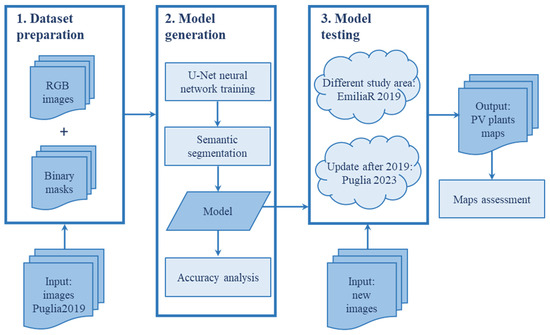
Figure 1.
A flowchart illustrating the primary stages of this study.
2.1. Study Areas
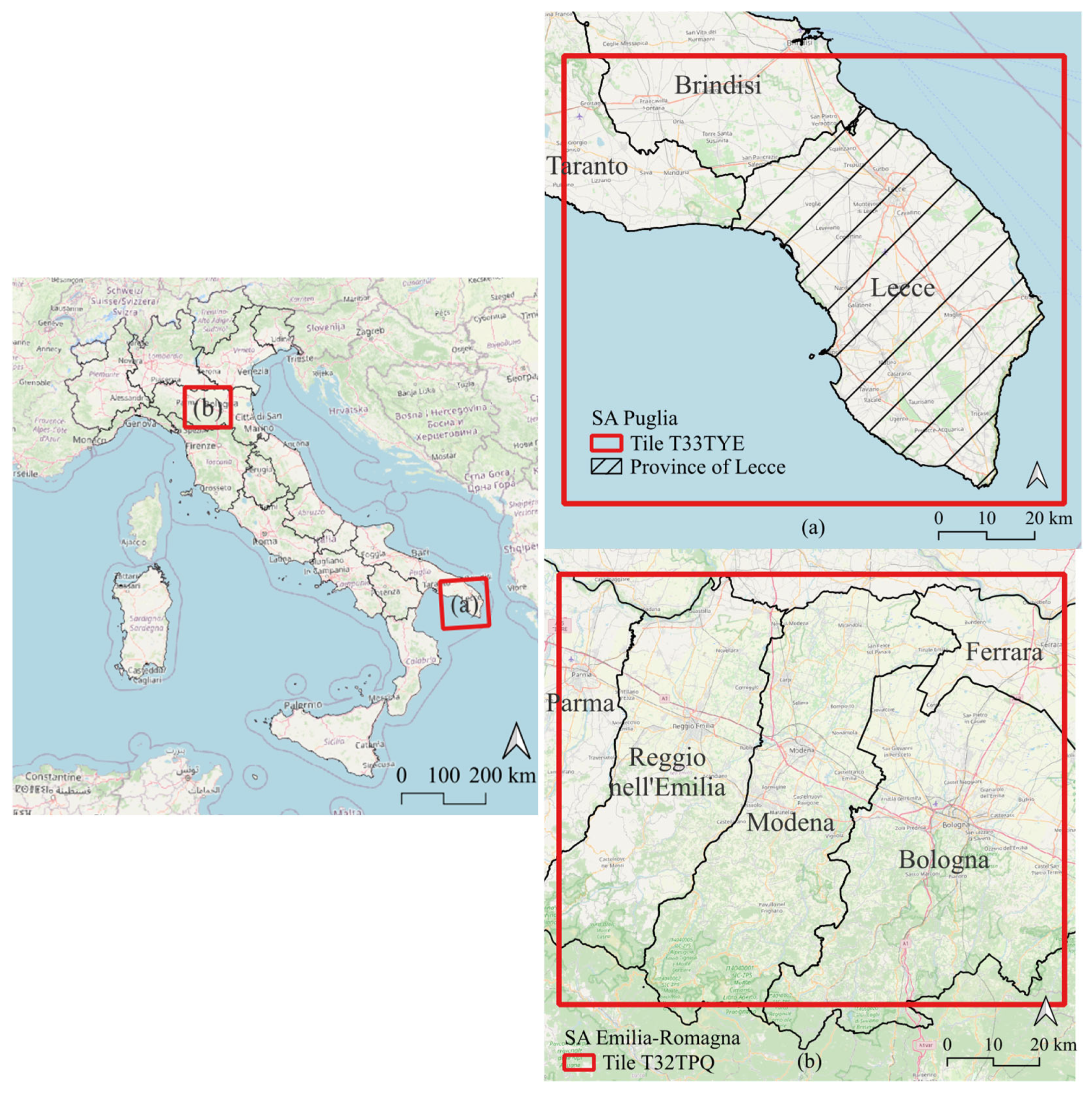
In recent years, the southern regions of Italy have experienced the most significant penetration of ground-mounted PV panels, with Puglia standing out as a notable example. By the end of 2023, ground-mounted systems accounted for 66% of the total PV systems in this region [44]. Puglia also stands out as the region with the highest total installed capacity and the largest average size of ground-mounted systems [44,45]. Northern regions, in contrast, exhibit a low penetration rate of ground-mounted system capacity, falling below 10% in the provinces of Liguria, Lombardia, Valle d’Aosta, and Trentino-Alto Adige. Thus, we choose to incorporate two distinct study areas in this research (refer to Figure 2), to be representative of different PV penetrations.
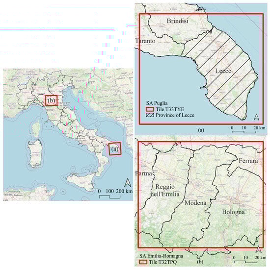
Figure 2.
Study areas: (a) SA Puglia, used for both model training and testing; (b) SA Emilia-Romagna, used for model testing. Basemap: @OpenStreetMap Contributors.
The first study area (hereby named SA Puglia) corresponds to Sentinel-2 tile T33TYE and covers the whole province of Lecce, as well as portions of Taranto and Brindisi. This study area was selected for both training and testing of the methodology, as it accounted for the highest concentration of photovoltaic power in 2023 and the highest amount of new PV installations among southern Italian provinces [44].
The second study area (hereby named SA Emilia-Romagna) corresponds to Sentinel-2 tile T32TPQ and is located between the Italian provinces of Modena, Reggio-Emilia, Bologna, Parma, and Ferrara. This study area was chosen for methodology testing, as characterized by a different morphological and geographical context with respect to the training environment. In addition, an official PV plant database is available for this study area in the regional high-resolution land use/land cover map [43].
2.2. Satellite Imagery
RGB Sentinel-2 images (L2A products) at 10 m spatial resolution downloaded from the Copernicus Data Space Ecosystem Browser [46] were used in this work. Cloud-free images (cloud cover percentage < 5%) were selected for the two study areas for the years 2019 and 2023. We considered all the available images acquired over the whole year to make the model robust to variations in the lighting conditions and seasonality of the surrounding territory. A detail of the images used for training and testing of the methodology for the two study areas is reported in Table 1. Sentinel-2 L2A images already provided surface reflectance values, yet some pre-processing was computed to the data. Pixels corresponding to small clouds and/or cloud shadows were masked out using the scene classification layer (SCL) provided within acquisitions. Additionally, where needed, seawater pixels were removed to prevent sea surface roughness brightness from interfering with the segmentation process.

Table 1.
Sentinel-2 imagery dataset used within this work.
To facilitate neural network training [15,23], RGB image tiles, each covering 110 × 110 km2, were split into sub-blocks of 549 × 549 pixels, equivalent to an area of approximately 30 km2.
2.3. Reference Dataset
In Italy, the most recent national mapping of ground-mounted PV installations (with capacity > 100 kW) was conducted in 2019 [42]. This mapping campaign involved the manual digitization of the footprints of PV systems, utilizing a collection of data points that encompassed the locations and technical specifications of the plants. Consequently, this national database, which includes the location, perimeter, and capacity of each installed PV system, served as the reference dataset for our methodology. During the model training phase, the dataset was used to generate labels to be associated with images for SA Puglia year 2019, while during the model testing phase, the dataset was used as a validation set to assess PV maps’ accuracy for both SA Puglia year 2023 and SA Emilia-Romagna year 2019. The number of PV plants and their power capacity are summarized in Table 2 and Table 3 for SA Puglia and SA Emilia-Romagna, respectively.
Table 2.
PV plants included in the reference dataset for SA Puglia. Source [42].
Table 3.
PV plants included in the reference dataset for SA Emilia-Romagna. Source [42].
2.4. Semantic Segmentation Model
Semantic segmentation is a widely used computer vision method that involves assigning class labels to the individual pixels of an image through the application of a deep learning (DL) algorithm. Consequently, a semantic segmentation model is responsible for identifying and categorizing objects within an image by accurately delineating their spatial extent.
To map solar plants in satellite images, we must be able to automatically detect them with good accuracy. For this scope, we trained a semantic segmentation model based on the DL encoder-decoder U-Net architecture developed by [41]. Such a multilayered symmetric architecture allows the artificial neural network to acquire more precise information, thanks to the fact that its structure can keep the learned information for longer by concatenating high-level features with low-level features. This process of concatenating information from various blocks allows U-Net to produce accurate results even with small training datasets.
The U-Net architecture includes an initial down-sampling path (i.e., encoder) that enables the neural network to extract contextual information and characteristics of the objects intended for segmentation within the image. Subsequently, a final up-sampling path (i.e., decoder) utilizes the information gathered in the first phase to accurately determine the locations of the objects and produce their segmentation as output.
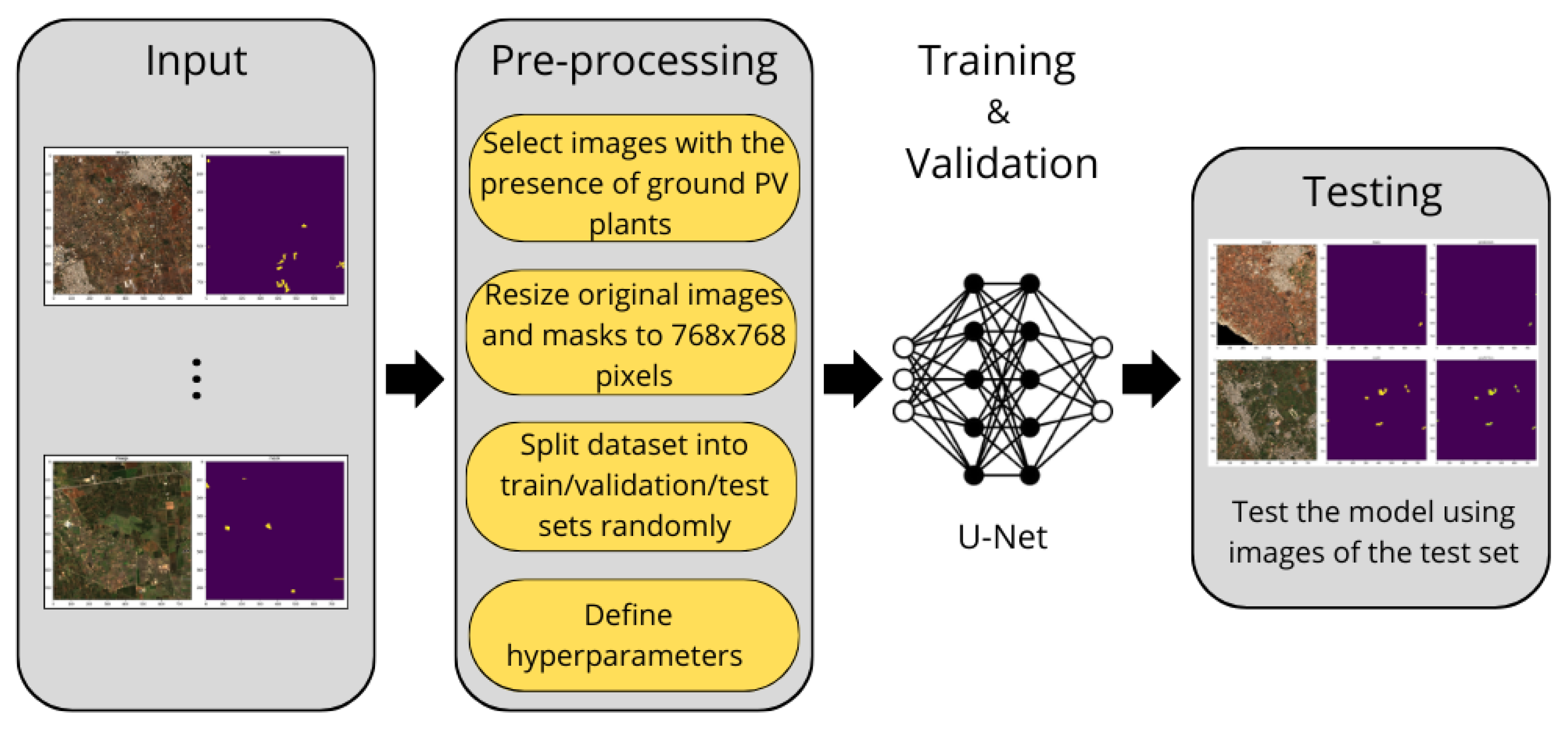
The model was trained to differentiate PV plants from the surrounding background. The training process was conducted on a virtual machine equipped with an Nvidia GPU Tesla V100 with 32 GB of RAM to enhance efficiency and minimize processing time (around 60 min). Figure 3 illustrates the framework we proposed to train the semantic segmentation model.
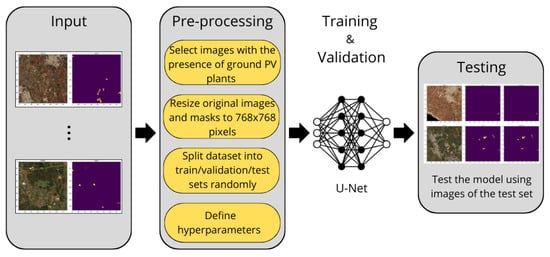
Figure 3.
Our proposed framework for the segmentation of PV installations on Sentinel-2 images.
2.4.1. Data Pre-Processing
The dataset used for model training counted 2397 RGB images along with their respective labels (see Section 2.2 and Section 2.3), each containing a minimum of one pixel labelled as a PV installation. Selected images referred to SA Puglia year 2019. The images and labels were resized from 549 × 549 pixels to 768 × 768 pixels to enhance the visibility of labelled segments, thereby assisting the model in detecting even the smallest portions of PV plants. Figure 4 shows an example of an RGB image, and its relative label used to train the semantic segmentation model. At this stage, we conducted the splitting of the complete dataset into training, validation, and test subsets with the following distribution: 60% allocated to the training set, 20% to the validation set, and 20% to the test set.
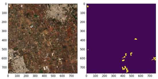
Figure 4.
An example of an RGB image and its corresponding label included in the dataset used for model training. Blue pixels represent background, yellow pixels represent PV plants.
2.4.2. Building of the Model
The segmentation model was developed with the U-Net architecture. This architecture is characterized by its symmetry, with both the encoder and the decoder consisting of four convolutional and deconvolutional blocks, each comprising two convolutional layers with an ReLU (rectified linear unit) as the activation function and a max pooling layer. The output is a convolutional layer, with Softmax as the activation function.
After preparing the training, validation, and test sets, we configured the hyperparameters. A summary of the selected values for each hyperparameter can be found in Table 4.
Table 4.
Hyperparameters configuration.
The model was trained minimizing cross-entropy (CE) chosen as loss function (Equation (1)):
where is the true probability distribution, and is the predicted probability distribution (output of Softmax).
The performance of the model during the training session was assessed using accuracy as the evaluation metric and checking the trend of the loss function.
2.5. Generating PV Plants Maps
In the third step of the methodology, the semantic segmentation model was tested on different case studies, namely SA Puglia 2023 and SA Emilia-Romagna 2019. We applied the model, using all the downloaded Sentinel-2 images (Table 1) as input, which resulted in many different outputs. The outputs generated by the model represented the likelihood of each pixel being classified as part of the PV class. Subsequent post-processing was performed to consolidate all model outputs and produce a final map depicting PV installations. Initially, the probability map outputs were converted into binary maps by applying a threshold of 60%. This threshold was determined empirically through an examination of pixel distribution histograms. Then, the maps were aggregated by summation, allowing each pixel to take on values ranging from 0 to N, with N equal to the number of satellite images used in SA. Ultimately, we normalized the result in relation to cloud masks to account for the presence of cloud or cloud shadows in the original imagery.
The results of the post-processing indicate the likelihood that a pixel corresponds to a PV plant, with values ranging from 0 to 100. A value of 0 represents no probability of being classified as PV, while a value of 100 represents a very high probability. To assess the efficacy of the methodology, thresholds of 0, 25, 50, 75, and 100 were applied. This strategy facilitates the analysis of classification effectiveness across different probability levels by producing PV maps for each specified threshold. These maps allow for a more comprehensive examination of the method’s ability to accurately identify PV plants at various confidence levels.
In addition, given the high number of plastic covered greenhouses (PCGs) that characterize the SA Puglia [47], we employed a simple method to identify PCGs and avoid potential misclassification with PV modules [48]. For this purpose, we computed the plastic greenhouse index (PGI) [49] on a Sentinel-2 image acquired in the summer season [50,51] for automatic mapping of PCGs and removed detected objects from the PV maps of thresholds 0 and 25.
Since the primary goal of this study is to identify the distribution of ground-mounted PV systems for optimized energy planning, it is essential to complement the mapping with data on the capacity of the PV modules. Thus, we first converted generated PV maps from raster format to vector format; then, we computed the extent of each detected plant and estimated capacity by mean of Equation (2):
where P is the capacity of a plant in megawatt [MW], A is the area occupied by a plant (expressed in km2), and Coeff is a coefficient representing the average ratio between area and capacity of existing plants, assumed equal to 0.018 km2 × MW−1.
P = A/Coeff,
2.6. Maps Validation
To validate final PV maps, the number and the extent of the identified installations were compared with the reference dataset (see Section 2.3) for both SA Puglia 2023 and SA Emilia-Romagna 2019. To focus the analysis on the methodology’s ability to recognize PV modules, we assessed accuracy metrics considering the class of PV plants only, without computing the performance for background pixel recognition. The validation was based on the calculation of accuracy scores (Equations (3)–(6)), namely user accuracy (UA), producer accuracy (PA), F1-score, and intersect over union (IoU):
where TP is the number of true positives, FP the number of false positives, and FN the number of false negatives. PA represents the map’s accuracy from the perspective of the map maker, indicating the proportion of correctly classified elements in a given class. UA reflects the map’s reliability from the user’s perspective, showing the proportion of elements labeled as a class on the map that truly belong to that class on the ground. The F1-score serves as a balanced evaluation metric that takes into account both PA and UA. IoU measures the degree of overlap between prediction and ground-truth [52]. Accuracy metrics were calculated based on the number of PV installations in the maps with respect to the reference dataset.
For SA Puglia 2023, we performed further assessments to evaluate how well the methodology works for updating maps and for estimating capacity. Capacity values derived from our maps were compared with values available from official statistics [44]. Since statistics are reported at the provincial (i.e., NUTS-3 [53]) scale, we validated results for the province of Lecce (see Figure 2). Finally, to assess the efficacy of detecting newly installed plants, we conducted a spatial intersection between reference data and model outputs and manually verified potential new photovoltaic installations, considering that the reference dataset is from 2019.
3. Results
3.1. Model Performances
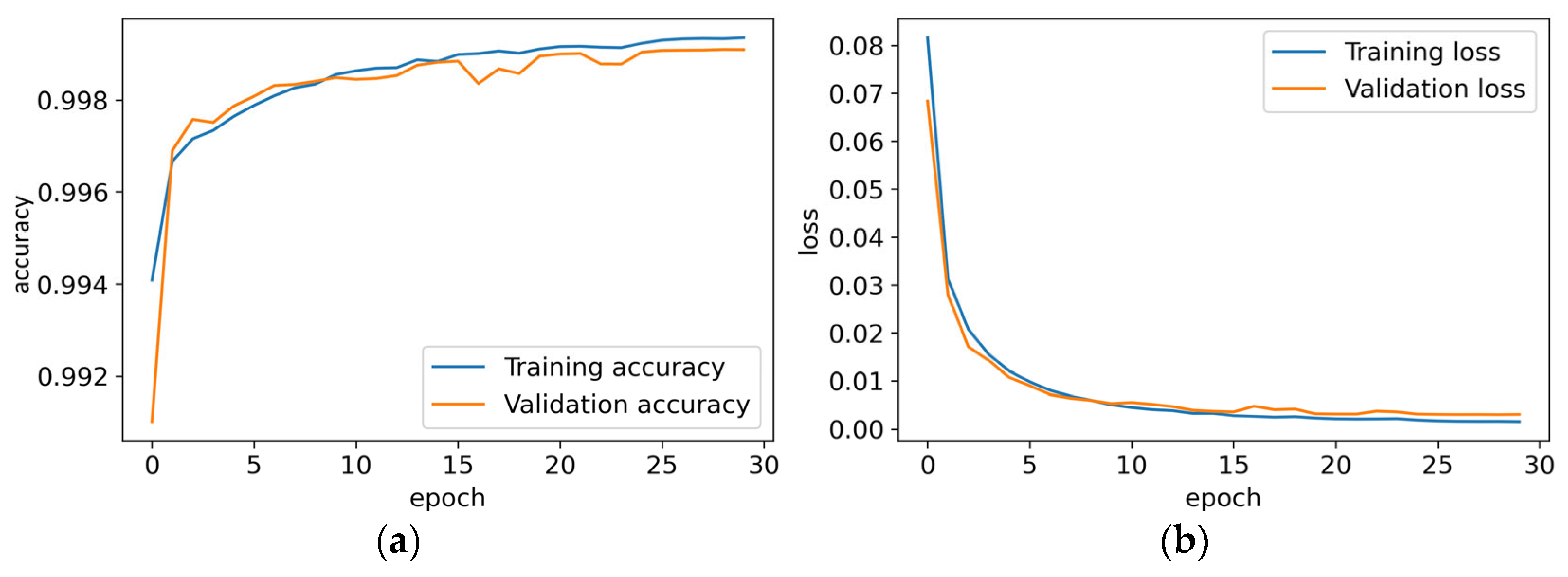
Figure 5 illustrates the learning curves of the model during the training phase. Additionally, Table 5 provides a summary of the accuracy and CE values achieved by the model at the end of the training process.
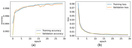
Figure 5.
The evaluation of accuracy and loss function during model training: (a) accuracy score curve, (b) cross-entropy curve.
Table 5.
Accuracy and loss function (cross-entropy) achieved during model training.
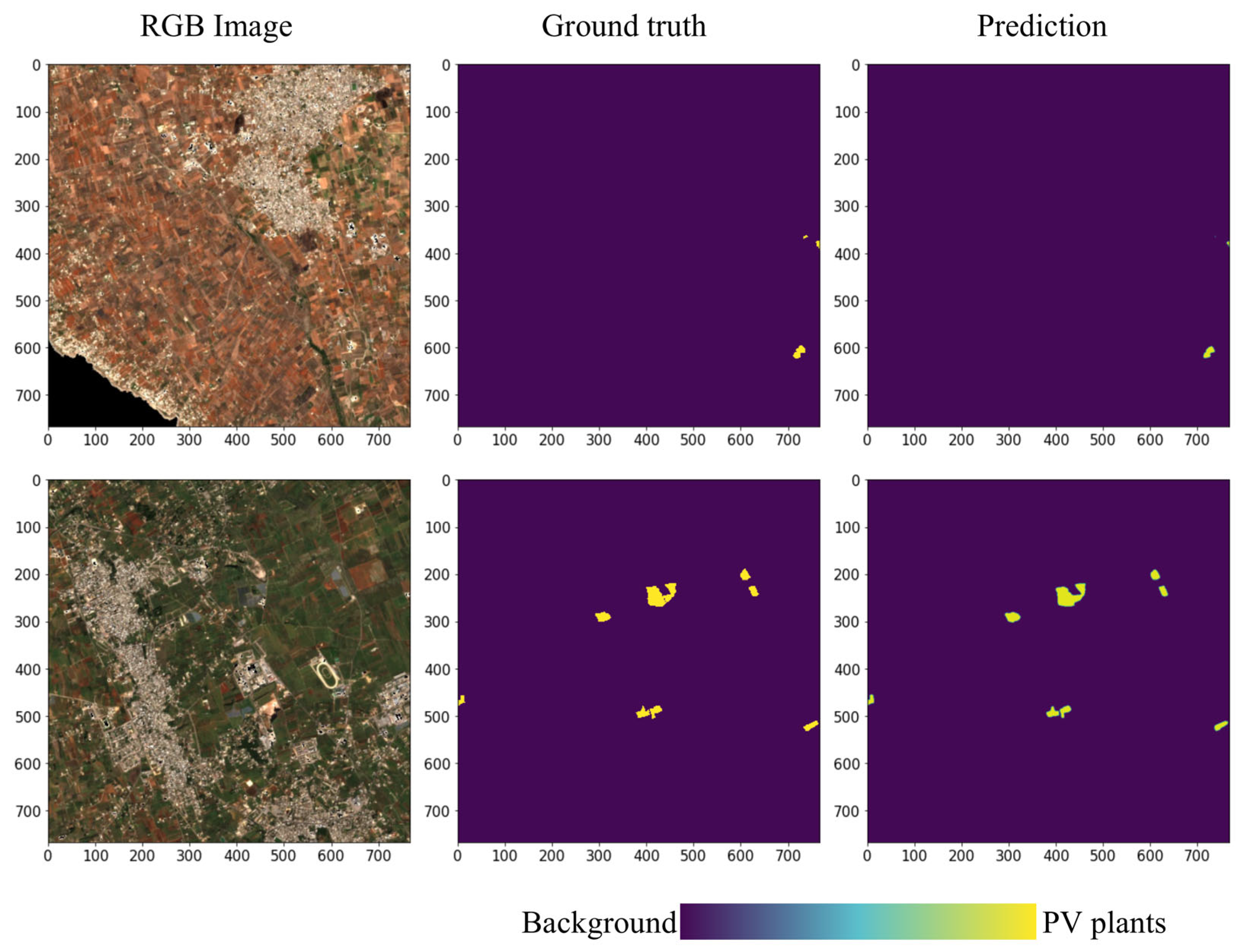
The high accuracy values achieved suggest that the model training was successful. Both the training and validation curves (Figure 5) follow a similar pattern, indicating that the model is well-fitted to the input dataset. Figure 6 represents two examples from the test set, with the RGB image on the left, ground truth in the middle, and model prediction on the right. Despite the notable differences between the two RGB images, the model accurately identifies PV modules with few errors along the edges, especially for smaller plants.

Figure 6.
Examples taken from the test set, representing RGB image, ground truth, and model prediction. Numbers in the maps indicate pixel coordinates [unitless].
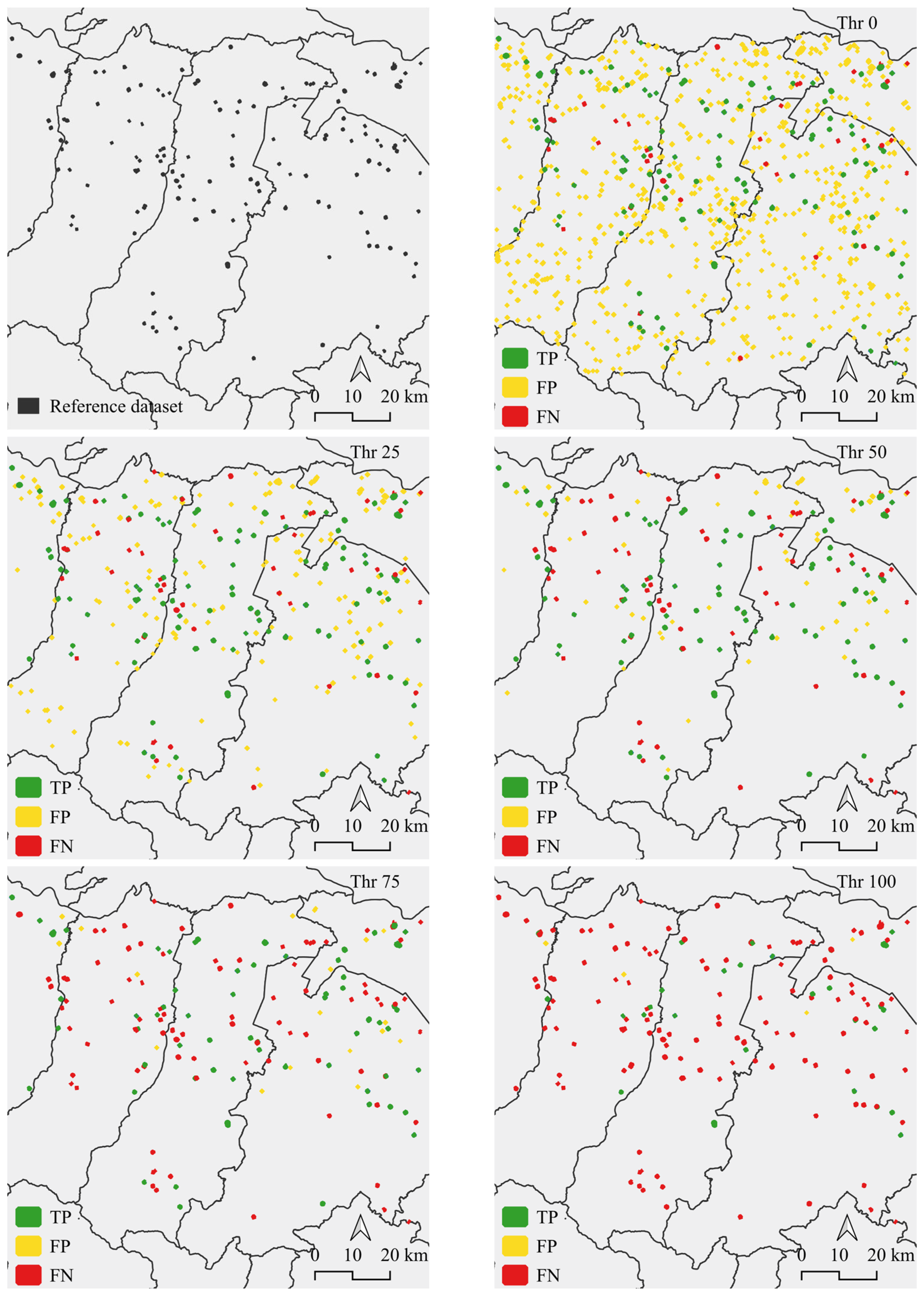
3.2. PV Plant Detection: SA Puglia
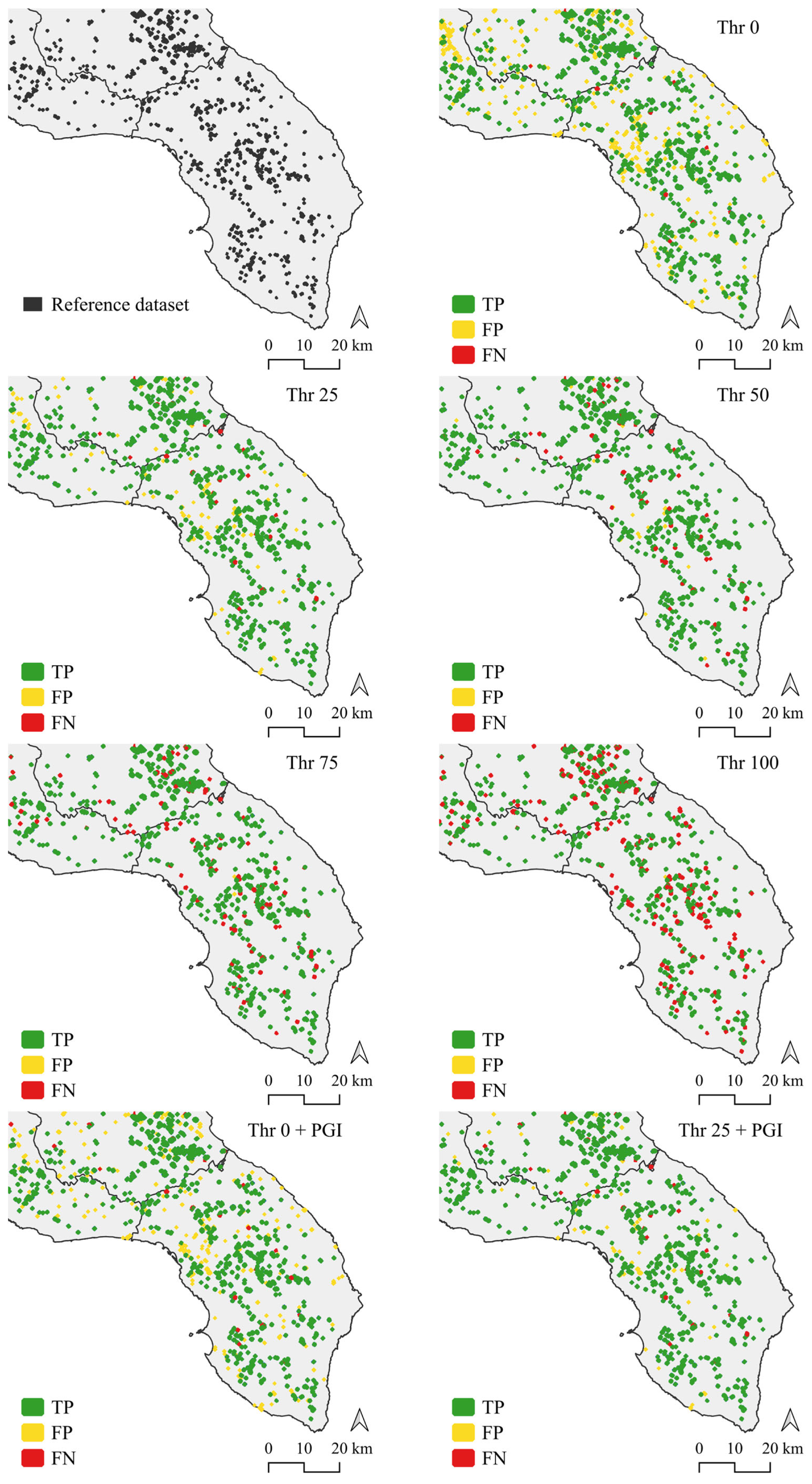
This section presents the outcomes obtained for the test SA Puglia (year 2023). Figure 7 displays PV plant maps obtained for varying threshold values. To enhance the understanding of map performances, we also present a map that illustrates the reference dataset. Overall, there is a good agreement between generated maps and the reference, indicating that the proposed methodology is effective for PV plant detection in this study area. Nonetheless, different results can be observed when considering the different thresholds. For low threshold values (i.e., 0 and 25), true positive detections predominate in the maps and false negatives are almost absent, while there are a great number of false positives, which implies an overestimation of PV installations, notably in the map for threshold 0. The reduction in false positives occurs with an increase in threshold values; however, this also leads to a decrease in true positives, resulting in a rise in false negatives and, consequently, a significant number of missed detections.
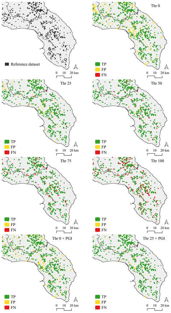
Figure 7.
SA Puglia 2023: PV plants maps obtained for varying threshold values.
The introduction of PGI also decreases the incidence of false positives while maintaining a high level of true positives. The outcomes depicted in the maps are confirmed by the accuracy scores reported in Table 6. Lower thresholds return the greatest PA values (>90%), while higher thresholds return the greatest UA values (close to 100%). Threshold 50 results in a good compromise, with the highest values for both F1-score and IoU. Using threshold 25 with PGI can reach comparable scores, since adding PGI leads to an increase in UA (+4%) with negligible effects on PA (−1%).
Table 6.
SA Puglia 2023: accuracy scores obtained for varying threshold values.
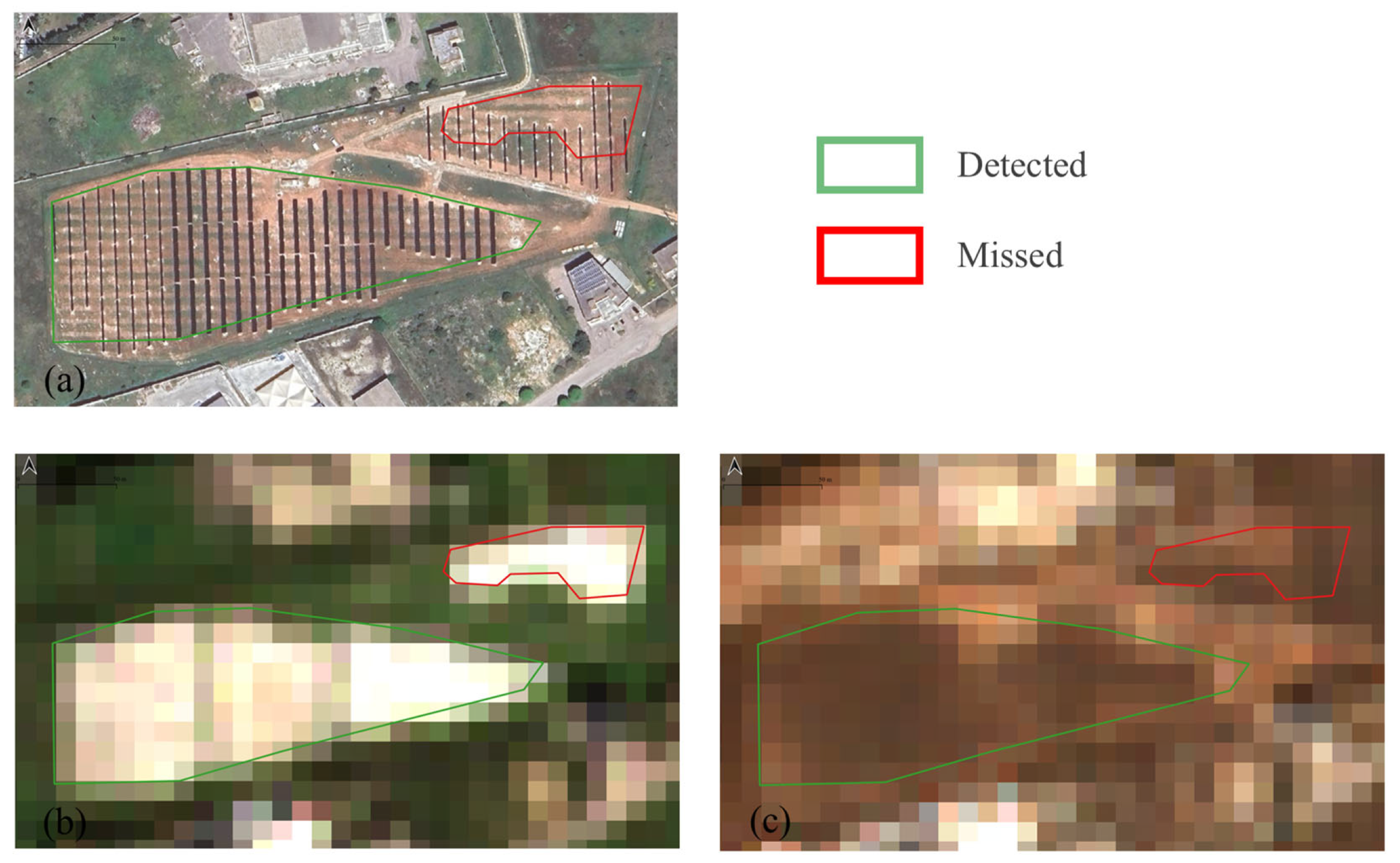
Although PA values exceed 90%, a few detections are missing in the maps. Some examples are reported in Appendix A (Figure A1, Figure A2 and Figure A3).
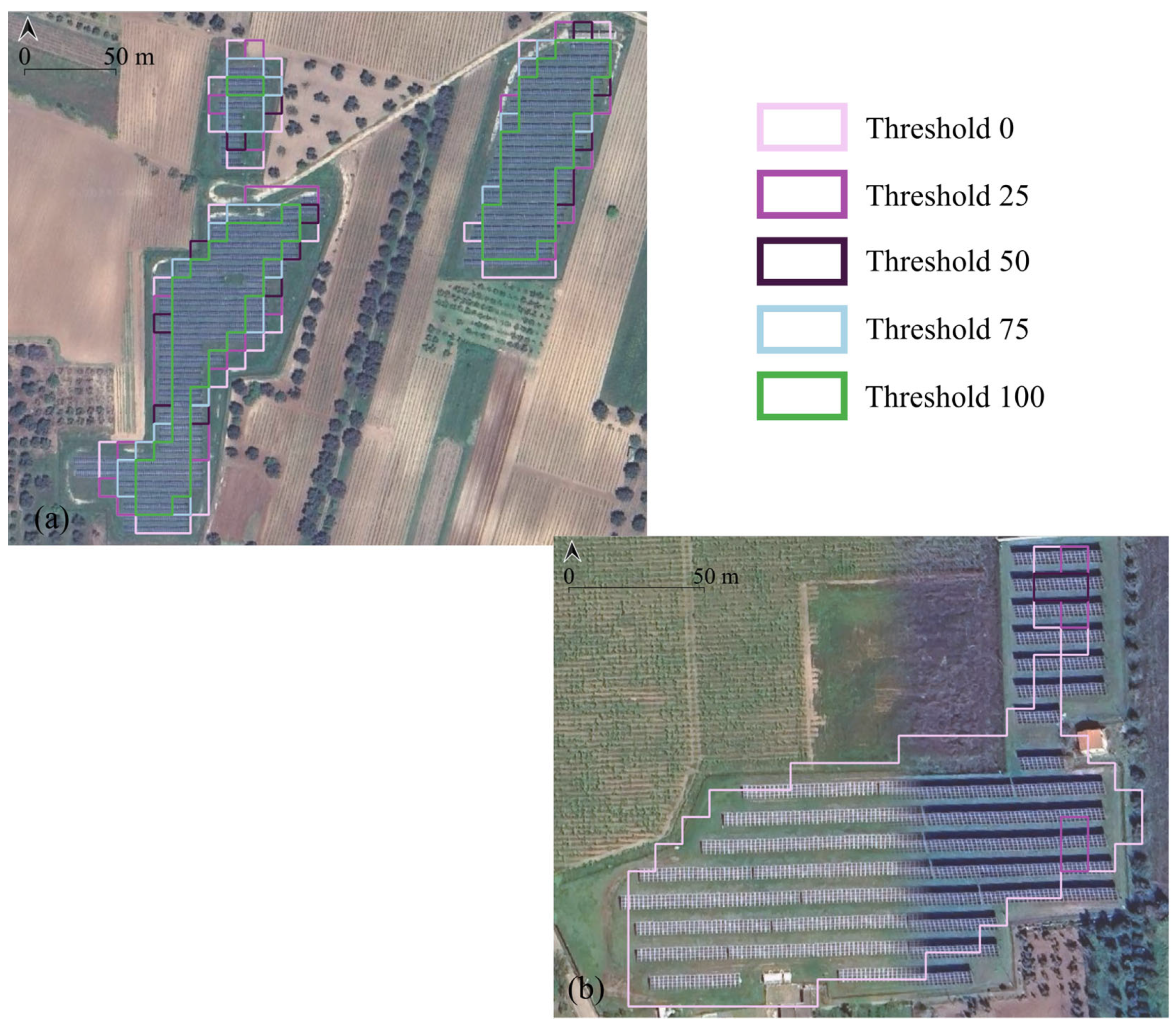
The aim of the methodology is to identify not only the sites of PV plants but also their size, enabling the estimation of power capacity based on the area-to-power relationship. Therefore, it is important to verify how the size of the plants varies as the threshold varies. Some examples are shown in Figure 8. In Figure 8a, PV installations are recognized with any threshold; plants edges are missing with higher threshold values, but overall, the full extent of PV farms is identified. Conversely, in Figure 8b, detection succeeds with thresholds lower than 50, but the whole shape of PV plants is fully reconstructed with threshold 0 only. The estimated capacity for varying threshold values is presented in Table 7. Figures refer to the province of Lecce, and the reference value (reported in official statistics) is around 540 MW for year 2023.
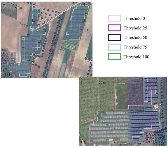
Figure 8.
Detection performances for varying threshold values: (a) examples of PV plants fully recognized with any threshold; (b) example of PV plants fully recognized only with threshold 0. Basemap: Google satellite.
Table 7.
Estimated capacity [MW] for varying threshold values. Assessment performed for the province of Lecce (reference value ~540 MW).
Maps generated with higher threshold values tend to underestimate the total PV capacity, even though they identify a similar number of plants to other maps. The reason behind this is that these thresholds identify only limited sections of PV plants, frequently dividing a single plant into multiple segments, which consequently diminishes the effectiveness of the maps for this study. On the other hand, maps produced with threshold equal to 0 (both with and without PGI) tend to overestimate total capacity due to an excess in the number of recognized installations and over-identification of plant extents. The map generated with a threshold of 50, which yields the highest accuracy ratings, tends to underestimate PV capacity. Although it is proficient in recognizing the locations of plants, this map encounters difficulties in accurately representing the size of the plants. The map created with a threshold of 25 comes closer to the reference value, especially when PGI is applied to reduce misclassification with plastic greenhouses.
Finally, we present performances in detecting potential new plants (Table 8).
Table 8.
Detection of potential new installations for varying threshold values. Potential new installations are retrieved as the difference of the spatial intersection between PV plant maps and the reference dataset dated to 2019.
Higher threshold values fail in detecting potential new plants, whereas low thresholds overestimate the number of potential new plants, as false positives predominate in the maps. The application of PGI appears to be advantageous, particularly as the total number of plants and the number of new plants decrease by an equivalent amount.
Figure 9 illustrates an example of new PV plants installed during year 2023. The plant depicted on the left is absent in the image captured in January (Figure 9b), but it is present in the image taken in October 2023 (Figure 9c). The proposed methodology employs a multi-temporal approach, incorporating semantic segmentation applied to different satellite images from the same year, which facilitates the accurate identification of this object on the maps at the lowest threshold values.

Figure 9.
Detection performances for varying threshold values: examples of PV plants as visible in the (a) Google Satellite basemap, the (b) Sentinel-2 image from January 2023, and the (c) Sentinel-2 image from October 2023.
3.3. PV Plant Detection: SA Emilia-Romagna
This section presents the outcomes obtained for the test SA Emilia-Romagna (year 2019). Accuracy scores are reported in Table 9.
Table 9.
SA Emilia-Romagna 2019: accuracy scores obtained for varying threshold values.
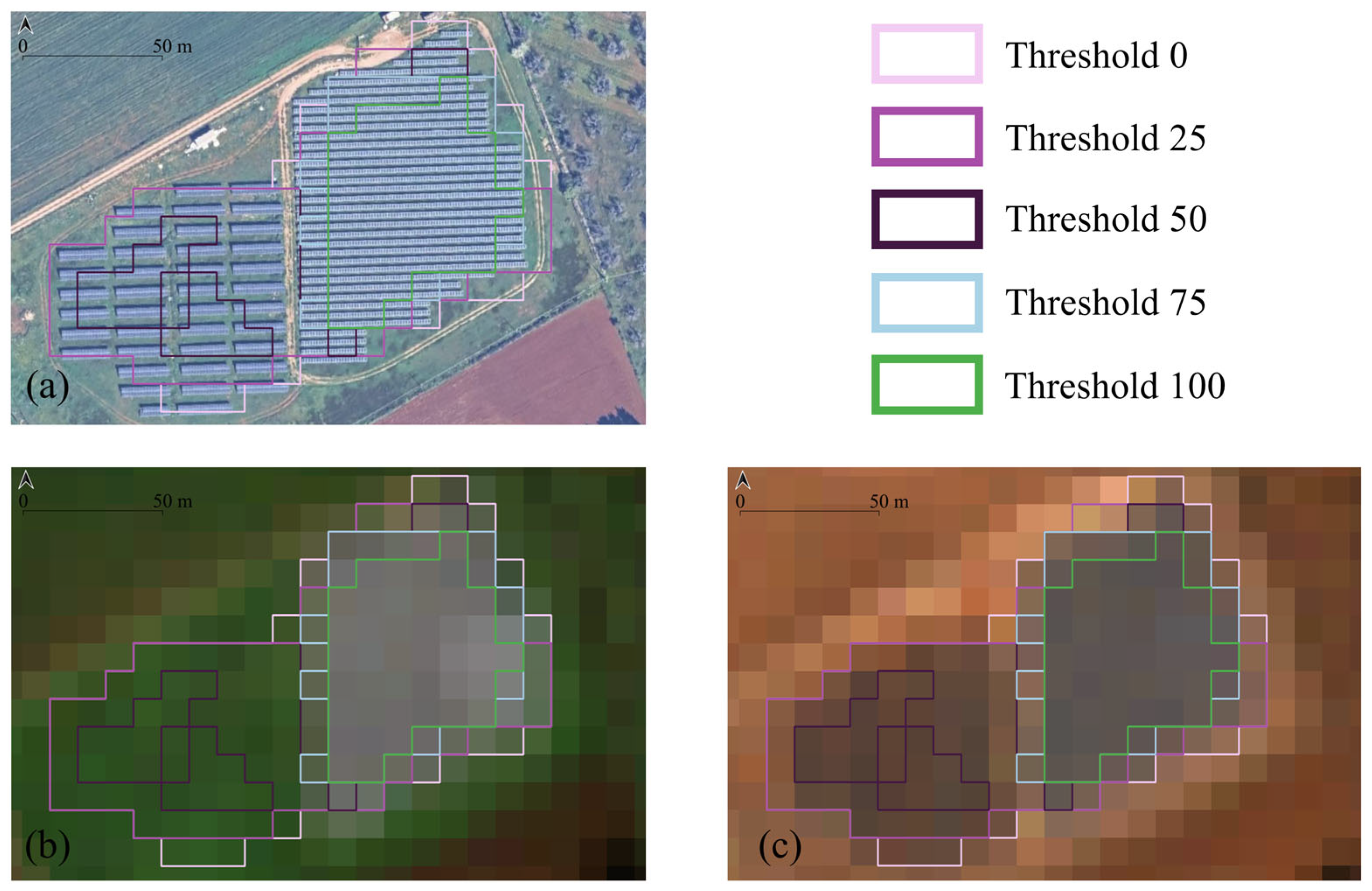
Figure 10 displays PV plant maps obtained for varying threshold values and a map representing the reference dataset. Overall, accuracy scores remain low, and significantly lower than the values calculated for the previous SA. The highest scores are achieved with the threshold equal to 50, yielding UA, PA, and an F1-score around 60%—less than the 90% obtained for SA Puglia. The observed trend is validated; at reduced thresholds, maps exhibit a higher occurrence of true positives and false positives, which results in high PA values and low UA values. As the threshold is raised, the number of false positives declines; nevertheless, there is a substantial increase in false negatives, leading to high UA values but low PA values.
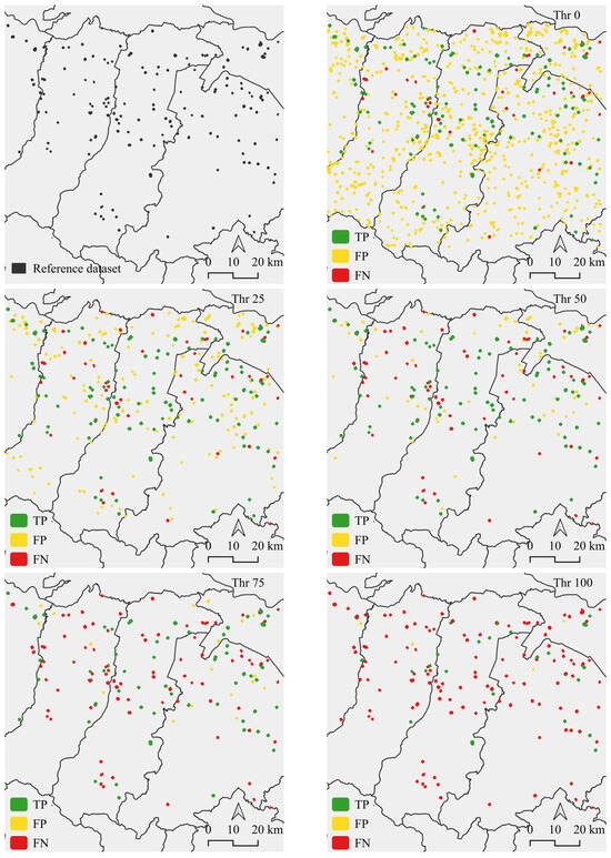
Figure 10.
SA Emilia-Romagna 2019: PV plants maps obtained for varying threshold values.
4. Discussion
4.1. Semantic Segmentation for PV Plant Detection
The learning curves resulting from the training phase show that our model was built correctly. Both training and validation curves follow a smooth behaviour, reaching convergence in 30 epochs. The number of images used for training is adequate, leading to better learning performances compared to [40]. Accuracies calculated on the validation set are close to the ones on the training set, reducing model overfitting, and in line with values reported in other studies, which are usually greater than 97% [32,34,54]. These results demonstrate a certain ability of semantic segmentation in detecting PV installations on satellite imagery. Nonetheless, authors warn of the main limitations of these methods, including difficulties in generalizing and extending the models—often too dependent on the specific characteristics of the images used during calibration—and high accuracy values derived from a significant imbalance between pixels representing PV plants and the background, which typically outnumber them considerably [23]. For these reasons, we assessed our model on cases different from the one on which it was trained.
Tests carried out for SA Puglia return high accuracy scores, proving good performances in PV objects recognition, with UA ranging from 63% to 100% and PA from 71% to 96% and a low rate of undetected plants. Those cases (see Appendix A) represent small PV farms, or less common layouts for PV installations, meaning that the model fails in recognizing them that and further training is needed. Moreover, PV modules smaller than the spatial resolution of Sentinel-2 images can generate missing detections due to the presence of mixed pixels that contain both PV and soil portions. To improve the model’s ability in detecting small objects, it would be appropriate to increase the spatial resolution of the input data, combining Sentinel-2 imagery (10 m resolution) with high-resolution images in a multi-scale and multi-source framework, as proposed by [23,35,54]. As an alternative, more exhaustive training datasets and new architectures could be investigated. Among others, Mask2Former, recently developed by [55], obtained excellent accuracies in segmenting various types of PV plants, from large-scale utility to small residential panels, outperforming U-Net results.
Finally, the methodology we proposed is based on a multi-temporal approach, where semantic segmentation is applied to multiple images captured within the same year. This approach has proven effective for detecting PV plants and allows users to select the most suitable mapping threshold according to their specific application needs. Lower thresholds help minimize the number of undetected objects (i.e., higher PA values), while higher thresholds reduce commission errors (i.e., higher UA values). An additional advantage of the multi-temporal approach is that accuracies remain consistent and are not influenced by the choice of input images. In [28], the greatest accuracy scores were achieved using spring images, while they decreased when including images from the autumn season. Our method, however, is season-independent, resulting in greater transferability, particularly when applied to different study areas with seasonal variations (e.g., predominance of winter crops vs. summer crops).
4.2. Mapping PV Plants in Different Landscapes
The model demonstrates high accuracy when tested on the same study area used for training. However, its performance declines noticeably when applied to a different study area, as indicated by a significant decrease in all assessment metrics for SA Emilia-Romagna. This suggests challenges in model generalizability. The primary difficulties stem from the diverse characteristics of the two areas, including variations in landscape and context, such as the prevalent morphology, the spatial distribution of PV plants, and the size of installations. The training area (i.e., Puglia) is characterized by extensive plains, a high density of ground-mounted PV systems, and large-scale PV farms, which contrasts with the differing attributes of the other area (i.e., Emilia-Romagna). Many studies report similar challenges when trying to transfer detecting models. Ref. [29] found that a classifier trained in highly urbanized coastal landscape outperformed a classifier trained in rural landscape. One possible solution they proposed is to use many regions during training, to achieve better accuracy scores. Similarly, ref. [37] also trained a machine learning pipeline with data from various study areas to generate a global model to identify PV modules.
Another limitation to model transfer could be related to the use of RGB images. To improve the recognition of PV systems and reduce omission errors, some authors suggest including multi-spectral data and combining the various spectral bands using simple algebraic formulas to obtain spectral indices [27,31]. In the literature, the most prevalent indices consist of vegetation indices (e.g., Bare Soil Index [56], Enhanced Vegetation Index [57], Normalized Difference Vegetation Index [58]), indices for assessing the water content on a surface (e.g., Land Surface Water Index [59], Normalized Difference Water Index [60], Normalized Difference Snow Index [61]), and indices for characterizing built environments (e.g., Built-Up Index [62], Normalized Difference Built-up Index [63]). Ground-mounted PV systems generally return low values for vegetation and water indices and high values for built-environment indices, in contrast to the background in which they are located (typically agricultural fields or sparsely vegetated areas), allowing for their distinction.
Moreover, some studies have shown that even greater accuracy in extracting PV systems can be achieved by combining spectral bands and indices with other types of data, such as texture variables [24,26], geometric and topographic information [39,64], or radar satellite images [25,28,29]. For the SA Emilia-Romagna test addressed in this study, further issues in PV plant detection could be attributed to a complex morphology, given that the mountainous terrain, mountain shadows, and bare rock soil can affect confusion errors. As already discussed in [39,51], we can expect performance improvements integrating satellite imagery with topographic data, namely digital terrain models, slope, and hillshade maps.
4.3. Mapping PV Plants for Energy Planning
This study aims at proposing a methodology to be used for generating PV plant maps for energy planning purposes. Therefore, it should be valid in detecting the locations of PV farms (as discussed in the previous sections), guarantee frequent updates, and allow for the estimation of capacity values. Our results demonstrate that semantic segmentation can be effective for the scope, especially when applied to satellite imagery with a multi-temporal approach and selecting maps with low threshold values. This approach guarantees on the one hand the detection of existing and potential new plants with good accuracy; on the other hand, it allows for the identification of the whole size of plants, including borders where mixed pixels prevail on the images, and derive capacity through the area-to-power relationship [65]. Maps from high threshold values hardly reconstruct the shape of objects, mainly due to different segmentation performances on the acquired images depending on season, background, and light conditions. Maps from low thresholds allow for PV plants identified in any of the original satellite image to be considered, thus ensuring continuity and increasing the number of detections.
Nonetheless, the main limitation with this approach consists of dealing with false positives, namely objects erroneously classified as PV installations. In this study, for SA Puglia, we managed to reduce misclassifications of plastic covered greenhouses with a proper filtering, since those elements characterized the area of interest. However, different objects could be addressed when extending the methodology to cover other regions in Italy [18,22]. Moreover, technological advances may bring new layouts and types of PV systems to the market. To ensure the effectiveness of the model in the future, it is important to keep the training dataset updated by including the latest developments. In the next years, an increase in agrivoltaic systems is expected [66], which may require a dedicated update in segmentation model training. By providing updated insights, this methodology will support energy planning strategies and help manage current and future potential of PV installations across Italy.
The achievement of high levels of decarbonization outlined in national and European plans requires the development of renewable energy resources and the optimized integration of various energy carriers to maximize generation. The adoption of modelling tools can aid in the planning and sustainable management of the energy system, monitoring the spatial and temporal variability of renewable resources, even in geographically complex contexts such as Italy. The methodology presented in this study will provide a more comprehensive understanding of the potential energy output from PV systems, enabling more effective planning and decision-making.
5. Conclusions
In recent years, the expansion of photovoltaic installations has accelerated, highlighting their crucial role as a renewable energy source in the global energy transition. However, comprehensive information on the spatial distribution of PV systems remains limited, posing challenges for effective energy planning.
This study introduces a methodology for automatic recognition of the location and extent of ground-mounted PV systems in Italy using semantic segmentation applied to 10 m resolution RGB images acquired from the Sentinel-2 satellites. The proposed model employs a U-Net architecture, achieving 99% accuracy during training, including the validation dataset. The methodology relies on a multi-temporal approach, deploying the semantic segmentation model on a set of images collected throughout the year. Model outputs are then aggregated into a final map representing the probability of PV plant detection. This method allows for flexible accuracy optimization, depending on the application needs: lower probability thresholds can be chosen to increase producer accuracy (PA), while higher thresholds improve user accuracy (UA). Furthermore, lower probability thresholds ensure continuous area detection, proving more effective in estimating PV power output using an area-to-power relationship. Such thresholds are also advantageous for identifying new installations, despite the trade-off of increased false positives, which can be mitigated through post-processing techniques, such as filters for recognising plastic-covered greenhouses.
Nevertheless, the proposed methodology has certain limitations. Detection of small installations is constrained by image resolution, as well as some specific PV plant layouts which necessitate a broader training dataset, more specialized model architectures, or the integration of additional spectral data. Another challenge lies in the model’s generalizability across diverse landscapes. To address this issue, future work will focus on re-training the model with images from various environmental contexts to facilitate PV plant recognition across different landscapes and PV configurations. Additionally, the complexity of terrain morphology has emerged as a significant obstacle; integrating topographic information, such as elevation maps, slope, and hillshade data, is proposed to enhance detection accuracy and robustness.
Author Contributions
Conceptualization, G.R. and M.A.; methodology, G.R., M.A. and A.M.; software, G.R. and A.M.; validation, G.R.; data curation, G.R. and A.M.; writing—original draft preparation, G.R. and M.A.; writing—review and editing, G.R., M.A. and A.M.; visualization, G.R. and M.A.; supervision, M.A. All authors have read and agreed to the published version of the manuscript.
Funding
This work has been financed by the Research Fund for the Italian Electrical System under the Three-Year Research Plan 2022–2024 (DM MITE n. 337, 15/09/2022), in compliance with the Decree of 16 April 2018.
Data Availability Statement
The datasets presented in this article are not readily available because the data are part of an ongoing study. Requests to access the datasets should be directed to corresponding author.
Acknowledgments
The authors would like to thank all colleagues whose comments improved the methodology presented in this paper.
Conflicts of Interest
The authors declare no conflicts of interest. The funders had no role in the design of the study; in the collection, analyses, or interpretation of data; in the writing of the manuscript; or in the decision to publish the results.
Appendix A
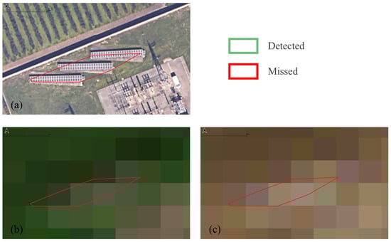
Figure A1.
Example of undetected small PV plants: (a) Google Satellite basemap; (b) Sentinel-2 image from January 2023; (c) Sentinel-2 image from October 2023.
Figure A1.
Example of undetected small PV plants: (a) Google Satellite basemap; (b) Sentinel-2 image from January 2023; (c) Sentinel-2 image from October 2023.
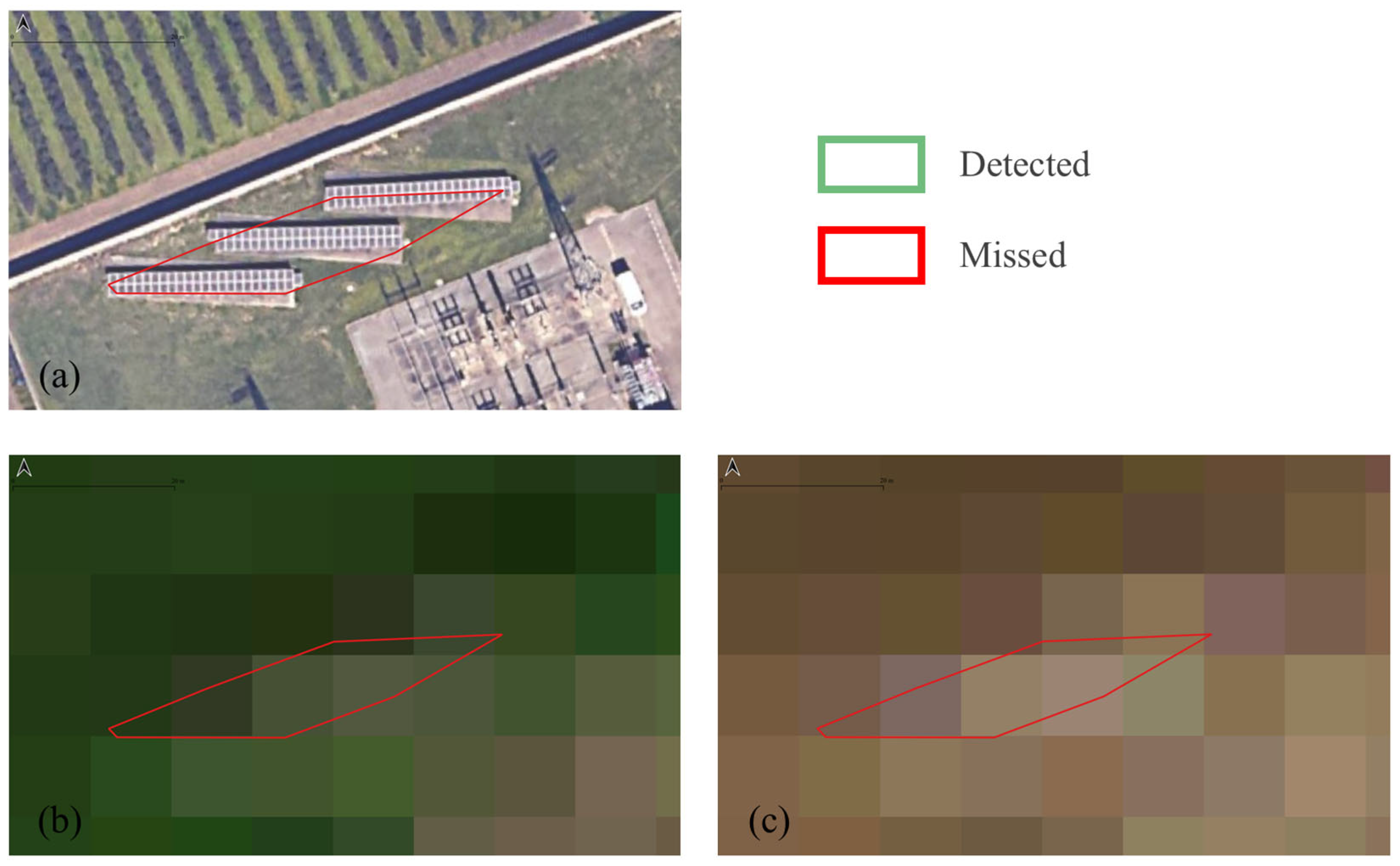

Figure A2.
Example of undetected PV plants: (a) Google Satellite basemap; (b) Sentinel-2 image from January 2023; (c) Sentinel-2 image from October 2023.
Figure A2.
Example of undetected PV plants: (a) Google Satellite basemap; (b) Sentinel-2 image from January 2023; (c) Sentinel-2 image from October 2023.
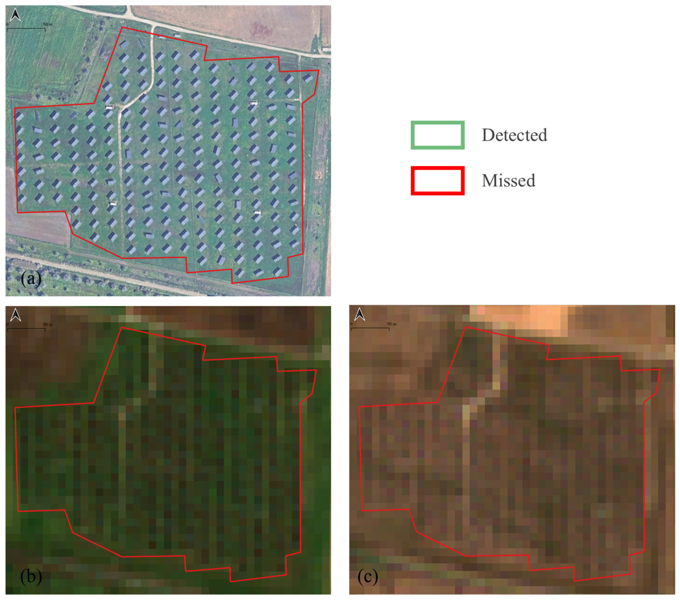
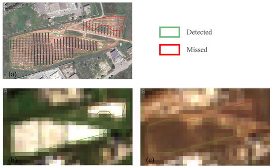
Figure A3.
Example of partially undetected PV plants: (a) Google Satellite basemap; (b) Sentinel-2 image from January 2023; (c) Sentinel-2 image from October 2023.
Figure A3.
Example of partially undetected PV plants: (a) Google Satellite basemap; (b) Sentinel-2 image from January 2023; (c) Sentinel-2 image from October 2023.
References
- Ministero dell’Ambiente e della Sicurezza Energetica (MASE). Piano Nazionale Integrato per l’Energia e il Clima 2024. Available online: https://www.mase.gov.it/sites/default/files/PNIEC_2024_revfin_01072024.pdf (accessed on 11 November 2024).
- European Union. Communication from the Commission to the European Parliament, the European Council, the Council, the European Economic and Social Committee and the Committee of the Regions Repowereu Plan; European Union: Brussels, Belgium, 2022. [Google Scholar]
- de Hoog, J.; Maetschke, S.; Ilfrich, P.; Kolluri, R.R. Using Satellite and Aerial Imagery for Identification of Solar PV: State of the Art and Research Opportunities. In Proceedings of the Eleventh ACM International Conference on Future Energy Systems, Virtual Event, 22–16 June 2020; Association for Computing Machinery: New York, NY, USA, 2020; pp. 308–313. [Google Scholar]
- Peters, R.; Berlekamp, J.; Tockner, K.; Zarfl, C. RePP Africa—A Georeferenced and Curated Database on Existing and Proposed Wind, Solar, and Hydropower Plants. Sci Data 2023, 10, 16. [Google Scholar] [CrossRef] [PubMed]
- Dunnett, S.; Sorichetta, A.; Taylor, G.; Eigenbrod, F. Harmonised Global Datasets of Wind and Solar Farm Locations and Power. Sci Data 2020, 7, 130. [Google Scholar] [CrossRef] [PubMed]
- Stowell, D.; Kelly, J.; Tanner, D.; Taylor, J.; Jones, E.; Geddes, J.; Chalstrey, E. A Harmonised, High-Coverage, Open Dataset of Solar Photovoltaic Installations in the UK. Sci Data 2020, 7, 394. [Google Scholar] [CrossRef] [PubMed]
- Claramunt, C.; Lotfian, M. Geomatics in the Era of Citizen Science. Geomatics 2023, 3, 364–366. [Google Scholar] [CrossRef]
- Heinisch, B. The Promises of Citizen Science—Fact or Fake? ARPHA Proc. 2024, 6, 13–18. [Google Scholar] [CrossRef]
- Chen, Q.; Li, X.; Zhang, Z.; Zhou, C.; Guo, Z.; Liu, Z.; Zhang, H. Remote Sensing of Photovoltaic Scenarios: Techniques, Applications and Future Directions. Appl. Energy 2023, 333, 120579. [Google Scholar] [CrossRef]
- Sun, T.; Shan, M.; Rong, X.; Yang, X. Estimating the Spatial Distribution of Solar Photovoltaic Power Generation Potential on Different Types of Rural Rooftops Using a Deep Learning Network Applied to Satellite Images. Appl. Energy 2022, 315, 119025. [Google Scholar] [CrossRef]
- Zhong, T.; Zhang, Z.; Chen, M.; Zhang, K.; Zhou, Z.; Zhu, R.; Wang, Y.; Lü, G.; Yan, J. A City-Scale Estimation of Rooftop Solar Photovoltaic Potential Based on Deep Learning. Appl. Energy 2021, 298, 117132. [Google Scholar] [CrossRef]
- Tiwari, A.; Meir, I.A.; Karnieli, A. Object-Based Image Procedures for Assessing the Solar Energy Photovoltaic Potential of Heterogeneous Rooftops Using Airborne LiDAR and Orthophoto. Remote Sens. 2020, 12, 223. [Google Scholar] [CrossRef]
- Hijjawi, U.; Lakshminarayana, S.; Xu, T.; Piero Malfense Fierro, G.; Rahman, M. A Review of Automated Solar Photovoltaic Defect Detection Systems: Approaches, Challenges, and Future Orientations. Sol. Energy 2023, 266, 112186. [Google Scholar] [CrossRef]
- Roggi, G.; Niccolai, A.; Grimaccia, F.; Lovera, M. A Computer Vision Line-Tracking Algorithm for Automatic UAV Photovoltaic Plants Monitoring Applications. Energies 2020, 13, 838. [Google Scholar] [CrossRef]
- Zhu, R.; Guo, D.; Wong, M.S.; Qian, Z.; Chen, M.; Yang, B.; Chen, B.; Zhang, H.; You, L.; Heo, J.; et al. Deep Solar PV Refiner: A Detail-Oriented Deep Learning Network for Refined Segmentation of Photovoltaic Areas from Satellite Imagery. Int. J. Appl. Earth Obs. Geoinf. 2023, 116, 103134. [Google Scholar] [CrossRef]
- Hou, X.; Wang, B.; Hu, W.; Yin, L.; Wu, H. SolarNet: A Deep Learning Framework to Map Solar Power Plants in China from Satellite Imagery. arXiv 2019, arXiv:1912.03685. [Google Scholar]
- Bradbury, K.; Saboo, R.; Johnson, T.L.; Malof, J.M.; Devarajan, A.; Zhang, W.; Collins, L.M.; Newell, R.G. Distributed Solar Photovoltaic Array Location and Extent Dataset for Remote Sensing Object Identification. Sci Data 2016, 3, 160106. [Google Scholar] [CrossRef] [PubMed]
- Jörges, C.; Vidal, H.S.; Hank, T.; Bach, H. Detection of Solar Photovoltaic Power Plants Using Satellite and Airborne Hyperspectral Imaging. Remote Sens. 2023, 15, 3403. [Google Scholar] [CrossRef]
- Malof, J.M.; Hou, R.; Collins, L.M.; Bradbury, K.; Newell, R. Automatic Solar Photovoltaic Panel Detection in Satellite Imagery. In Proceedings of the 2015 International Conference on Renewable Energy Research and Applications (ICRERA), Palermo, Italy, 22–25 November 2015; pp. 1428–1431. [Google Scholar]
- Czirjak, D.W. Detecting Photovoltaic Solar Panels Using Hyperspectral Imagery and Estimating Solar Power Production. JARS 2017, 11, 026007. [Google Scholar] [CrossRef]
- Cerra, D.; Ji, C.; Heiden, U. Solar Panels Area Estimation Using the Spaceborne Imaging Spectrometer Desis: Outperforming Multispectral Sensors. ISPRS Ann. Photogramm. Remote Sens. Spat. Inf. Sci. 2022, 1, 9–14. [Google Scholar] [CrossRef]
- Ji, C.; Bachmann, M.; Esch, T.; Feilhauer, H.; Heiden, U.; Heldens, W.; Hueni, A.; Lakes, T.; Metz-Marconcini, A.; Schroedter-Homscheidt, M.; et al. Solar Photovoltaic Module Detection Using Laboratory and Airborne Imaging Spectroscopy Data. Remote Sens. Environ. 2021, 266, 112692. [Google Scholar] [CrossRef]
- Guo, Z.; Zhuang, Z.; Tan, H.; Liu, Z.; Li, P.; Lin, Z.; Shang, W.-L.; Zhang, H.; Yan, J. Accurate and Generalizable Photovoltaic Panel Segmentation Using Deep Learning for Imbalanced Datasets. Renew. Energy 2023, 219, 119471. [Google Scholar] [CrossRef]
- Wang, X.; Xiao, X.; Zhang, X.; Ye, H.; Dong, J.; He, Q.; Wang, X.; Liu, J.; Li, B.; Wu, J. Characterization and Mapping of Photovoltaic Solar Power Plants by Landsat Imagery and Random Forest: A Case Study in Gansu Province, China. J. Clean. Prod. 2023, 417, 138015. [Google Scholar] [CrossRef]
- Jiang, W.; Tian, B.; Duan, Y.; Chen, C.; Hu, Y. Rapid Mapping and Spatial Analysis on the Distribution of Photovoltaic Power Stations with Sentinel-1&2 Images in Chinese Coastal Provinces. Int. J. Appl. Earth Obs. Geoinf. 2023, 118, 103280. [Google Scholar] [CrossRef]
- Chen, Z.; Kang, Y.; Sun, Z.; Wu, F.; Zhang, Q. Extraction of Photovoltaic Plants Using Machine Learning Methods: A Case Study of the Pilot Energy City of Golmud, China. Remote Sens. 2022, 14, 2697. [Google Scholar] [CrossRef]
- Ortiz, A.; Negandhi, D.; Mysorekar, S.R.; Nagaraju, S.K.; Kiesecker, J.; Robinson, C.; Bhatia, P.; Khurana, A.; Wang, J.; Oviedo, F.; et al. An Artificial Intelligence Dataset for Solar Energy Locations in India. Sci Data 2022, 9, 497. [Google Scholar] [CrossRef] [PubMed]
- Plakman, V.; Rosier, J.; van Vliet, J. Solar Park Detection from Publicly Available Satellite Imagery. GISci. Remote Sens. 2022, 59, 462–481. [Google Scholar] [CrossRef]
- Wang, J.; Liu, J.; Li, L. Detecting Photovoltaic Installations in Diverse Landscapes Using Open Multi-Source Remote Sensing Data. Remote Sens. 2022, 14, 6296. [Google Scholar] [CrossRef]
- Xia, Z.; Li, Y.; Chen, R.; Sengupta, D.; Guo, X.; Xiong, B.; Niu, Y. Mapping the Rapid Development of Photovoltaic Power Stations in Northwestern China Using Remote Sensing. Energy Rep. 2022, 8, 4117–4127. [Google Scholar] [CrossRef]
- Zhang, X.; Xu, M.; Wang, S.; Huang, Y.; Xie, Z. Mapping Photovoltaic Power Plants in China Using Landsat, Random Forest, and Google Earth Engine. Earth Syst. Sci. Data 2022, 14, 3743–3755. [Google Scholar] [CrossRef]
- Costa, M.V.C.V.d.; Carvalho, O.L.F.d.; Orlandi, A.G.; Hirata, I.; Albuquerque, A.O.d.; Silva, F.V.e.; Guimarães, R.F.; Gomes, R.A.T.; Júnior, O.A.d.C. Remote Sensing for Monitoring Photovoltaic Solar Plants in Brazil Using Deep Semantic Segmentation. Energies 2021, 14, 2960. [Google Scholar] [CrossRef]
- Kouyama, T.; Imamoglu, N.; Imai, M.; Nakamura, R. Verifying Rapid Increasing of Mega-Solar PV Power Plants in Japan by Applying a CNN-Based Classification Method to Satellite Images. In Proceedings of the IGARSS 2020—2020 IEEE International Geoscience and Remote Sensing Symposium, Waikoloa, HI, USA, 26 September–2 October 2020; pp. 4104–4107. [Google Scholar]
- Jurakuziev, D.; Jumaboev, S.; Lee, M. A Framework to Estimate Generating Capacities of PV Systems Using Satellite Imagery Segmentation. Eng. Appl. Artif. Intell. 2023, 123, 106186. [Google Scholar] [CrossRef]
- Kleebauer, M.; Marz, C.; Reudenbach, C.; Braun, M. Multi-Resolution Segmentation of Solar Photovoltaic Systems Using Deep Learning. Remote Sens. 2023, 15, 5687. [Google Scholar] [CrossRef]
- Yu, J.; Wang, Z.; Majumdar, A.; Rajagopal, R. DeepSolar: A Machine Learning Framework to Efficiently Construct a Solar Deployment Database in the United States. Joule 2018, 2, 2605–2617. [Google Scholar] [CrossRef]
- Kruitwagen, L.; Story, K.T.; Friedrich, J.; Byers, L.; Skillman, S.; Hepburn, C. A Global Inventory of Photovoltaic Solar Energy Generating Units. Nature 2021, 598, 604–610. [Google Scholar] [CrossRef] [PubMed]
- Breiman, L. Random Forests. Mach. Learn. 2001, 45, 5–32. [Google Scholar] [CrossRef]
- Zhang, X.; Zeraatpisheh, M.; Rahman, M.M.; Wang, S.; Xu, M. Texture Is Important in Improving the Accuracy of Mapping Photovoltaic Power Plants: A Case Study of Ningxia Autonomous Region, China. Remote Sens. 2021, 13, 3909. [Google Scholar] [CrossRef]
- Ioannou, K.; Myronidis, D. Automatic Detection of Photovoltaic Farms Using Satellite Imagery and Convolutional Neural Networks. Sustainability 2021, 13, 5323. [Google Scholar] [CrossRef]
- Ronneberger, O.; Fischer, P.; Brox, T. U-Net: Convolutional Networks for Biomedical Image Segmentation. In Proceedings of the Medical Image Computing and Computer-Assisted Intervention—MICCAI 2015, Munich, Germany, 5–9 October 2015; Navab, N., Hornegger, J., Wells, W.M., Frangi, A.F., Eds.; Springer International Publishing: Cham, Switzerland, 2015; pp. 234–241. [Google Scholar]
- Garofalo, E.; Aiello, M.; Airoldi, D.; Gargiulo, A. Definizione e Quantificazione delle Aree Idonee: Elementi di Discussione e Sperimentazione con la Regione Piemonte; RSE: Milano, Italy, 2021. [Google Scholar]
- 2020—Coperture Vettoriali Uso del Suolo di Dettaglio—Edizione 2023—Geoportale. Available online: https://geoportale.regione.emilia-romagna.it/download/dati-e-prodotti-cartografici-preconfezionati/pianificazione-e-catasto/uso-del-suolo/2020-coperture-vettoriali-uso-del-suolo-di-dettaglio-edizione-2023 (accessed on 8 November 2024).
- GSE. Gestore dei Servizi Energetici S.p.A. Rapporto Statistico 2023. Solare Fotovoltaico; Gestore dei Servizi Energetici S.p.A.: Roma, Italy, 2024. [Google Scholar]
- ISPRA. Consumo di Suolo, Dinamiche Territoriali e Servizi Ecosistemici. Edizione 2022—SNPA—Sistema Nazionale Protezione Ambiente 2022. Available online: https://www.snpambiente.it/snpa/consumo-di-suolo-dinamiche-territoriali-e-servizi-ecosistemici-edizione-2022/ (accessed on 11 November 2024).
- Copernicus Browser. Available online: https://browser.dataspace.copernicus.eu/ (accessed on 11 November 2024).
- Veettil, B.K.; Van, D.D.; Quang, N.X.; Hoai, P.N. Remote Sensing of Plastic-Covered Greenhouses and Plastic-Mulched Farmlands: Current Trends and Future Perspectives. Land Degrad. Dev. 2023, 34, 591–609. [Google Scholar] [CrossRef]
- Aguilar, M.A.; Jiménez-Lao, R.; Aguilar, F.J. Evaluation of Object-Based Greenhouse Mapping Using WorldView-3 VNIR and SWIR Data: A Case Study from Almería (Spain). Remote Sens. 2021, 13, 2133. [Google Scholar] [CrossRef]
- Yang, D.; Chen, J.; Zhou, Y.; Chen, X.; Chen, X.; Cao, X. Mapping Plastic Greenhouse with Medium Spatial Resolution Satellite Data: Development of a New Spectral Index. ISPRS J. Photogramm. Remote Sens. 2017, 128, 47–60. [Google Scholar] [CrossRef]
- la Cecilia, D.; Tom, M.; Stamm, C.; Odermatt, D. Pixel-Based Mapping of Open Field and Protected Agriculture Using Constrained Sentinel-2 Data. ISPRS Open J. Photogramm. Remote Sens. 2023, 8, 100033. [Google Scholar] [CrossRef]
- Zhang, P.; Du, P.; Guo, S.; Zhang, W.; Tang, P.; Chen, J.; Zheng, H. A Novel Index for Robust and Large-Scale Mapping of Plastic Greenhouse from Sentinel-2 Images. Remote Sens. Environ. 2022, 276, 113042. [Google Scholar] [CrossRef]
- Nicolau, A.P.; Dyson, K.; Saah, D.; Clinton, N. Accuracy Assessment: Quantifying Classification Quality. In Cloud-Based Remote Sensing with Google Earth Engine: Fundamentals and Applications; Cardille, J.A., Crowley, M.A., Saah, D., Clinton, N.E., Eds.; Springer International Publishing: Cham, Switzerland, 2024; pp. 135–145. ISBN 978-3-031-26588-4. [Google Scholar]
- Overview—Eurostat. Available online: https://ec.europa.eu/eurostat/web/nuts (accessed on 8 November 2024).
- Ge, F.; Wang, G.; He, G.; Zhou, D.; Yin, R.; Tong, L. A Hierarchical Information Extraction Method for Large-Scale Centralized Photovoltaic Power Plants Based on Multi-Source Remote Sensing Images. Remote Sens. 2022, 14, 4211. [Google Scholar] [CrossRef]
- García, G.; Aparcedo, A.; Nayak, G.K.; Ahmed, T.; Shah, M.; Li, M. Generalized Deep Learning Model for Photovoltaic Module Segmentation from Satellite and Aerial Imagery. Sol. Energy 2024, 274, 112539. [Google Scholar] [CrossRef]
- Diek, S.; Fornallaz, F.; Schaepman, M.E.; De Jong, R. Barest Pixel Composite for Agricultural Areas Using Landsat Time Series. Remote Sens. 2017, 9, 1245. [Google Scholar] [CrossRef]
- Huete, A.; Didan, K.; Miura, T.; Rodriguez, E.P.; Gao, X.; Ferreira, L.G. Overview of the Radiometric and Biophysical Performance of the MODIS Vegetation Indices. Remote Sens. Environ. 2002, 83, 195–213. [Google Scholar] [CrossRef]
- Rouse, J.W., Jr.; Haas, R.H.; Schell, J.A.; Deering, D.W. Monitoring Vegetation Systems in the Great Plains with ERTS. NASA Spec. Publ. 1974, 351, 309. [Google Scholar]
- Chandrasekar, K.; Sesha Sai, M.V.R.; Roy, P.S.; Dwevedi, R.S. Land Surface Water Index (LSWI) Response to Rainfall and NDVI Using the MODIS Vegetation Index Product. Int. J. Remote Sens. 2010, 31, 3987–4005. [Google Scholar] [CrossRef]
- McFEETERS, S.K. The Use of the Normalized Difference Water Index (NDWI) in the Delineation of Open Water Features. Int. J. Remote Sens. 1996, 17, 1425–1432. [Google Scholar] [CrossRef]
- Hall, D.K.; Riggs, G.A. Normalized-Difference Snow Index (NDSI). In Encyclopedia of Snow, Ice and Glaciers; Springer: Berlin/Heidelberg, Germany, 2013. [Google Scholar]
- He, C.; Shi, P.; Xie, D.; Zhao, Y. Improving the Normalized Difference Built-up Index to Map Urban Built-up Areas Using a Semiautomatic Segmentation Approach. Remote Sens. Lett. 2010, 1, 213–221. [Google Scholar] [CrossRef]
- Zha, Y.; Gao, J.; Ni, S. Use of Normalized Difference Built-up Index in Automatically Mapping Urban Areas from TM Imagery. Int. J. Remote Sens. 2003, 24, 583–594. [Google Scholar] [CrossRef]
- Wang, Y.; Cai, D.; Chen, L.; Yang, L.; Ge, X.; Peng, L. A Downscaling Methodology for Extracting Photovoltaic Plants with Remote Sensing Data: From Feature Optimized Random Forest to Improved HRNet. Remote Sens. 2023, 15, 4931. [Google Scholar] [CrossRef]
- Jie, Y.; Ji, X.; Yue, A.; Chen, J.; Deng, Y.; Chen, J.; Zhang, Y. Combined Multi-Layer Feature Fusion and Edge Detection Method for Distributed Photovoltaic Power Station Identification. Energies 2020, 13, 6742. [Google Scholar] [CrossRef]
- Ronchetti, G.; Galbiati, I.; Garofalo, E. Analyzing Wind and Photovoltaic Plant Development towards the Energy Transition in Italy. Next Energy, 2024; submitted. [Google Scholar]


Disclaimer/Publisher’s Note: The statements, opinions and data contained in all publications are solely those of the individual author(s) and contributor(s) and not of MDPI and/or the editor(s). MDPI and/or the editor(s) disclaim responsibility for any injury to people or property resulting from any ideas, methods, instructions or products referred to in the content. |
© 2025 by the authors. Licensee MDPI, Basel, Switzerland. This article is an open access article distributed under the terms and conditions of the Creative Commons Attribution (CC BY) license (https://creativecommons.org/licenses/by/4.0/).