

Machine Learning-Based Cerrado Land Cover Classification Using PlanetScope Imagery


Abstract

1. Introduction
2. Materials and Methods
2.1. Study Site
2.2. Field Data
2.3. Satellite Data and Feature Space
2.4. Machine Learning Classification Methods
2.5. Data Processing and Classification
2.6. Post-Classification
2.7. Accuracy Assessment
2.8. Land Cover Change
3. Results
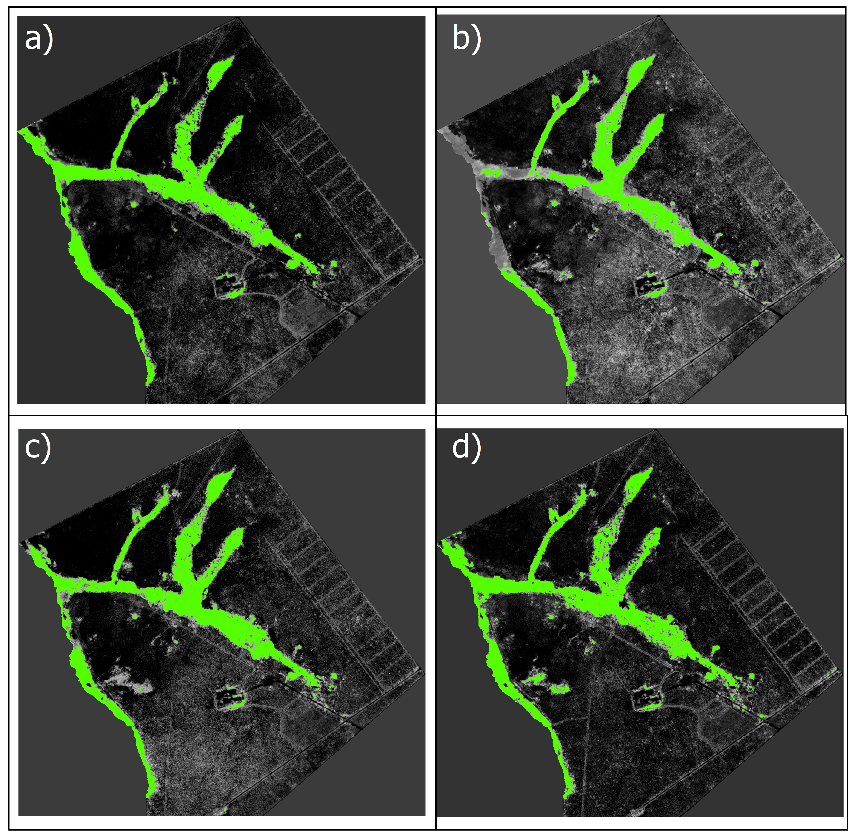
3.1. Mask Creation
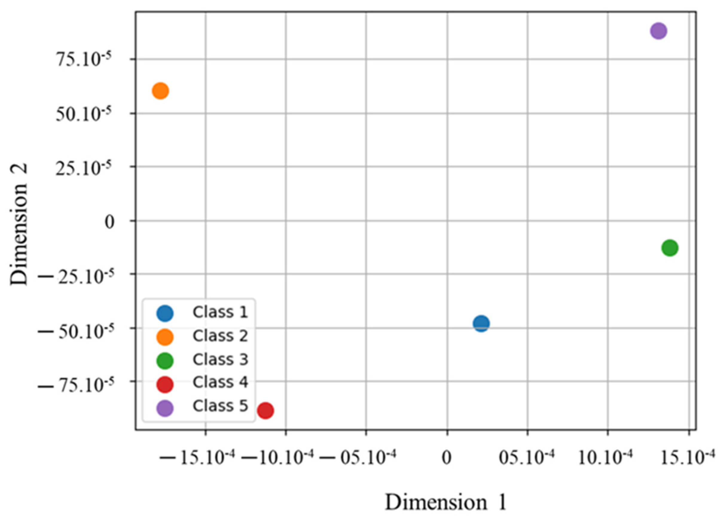
3.2. Class Separability
3.3. ML Classification Assessment
3.4. Accuracy Evaluation
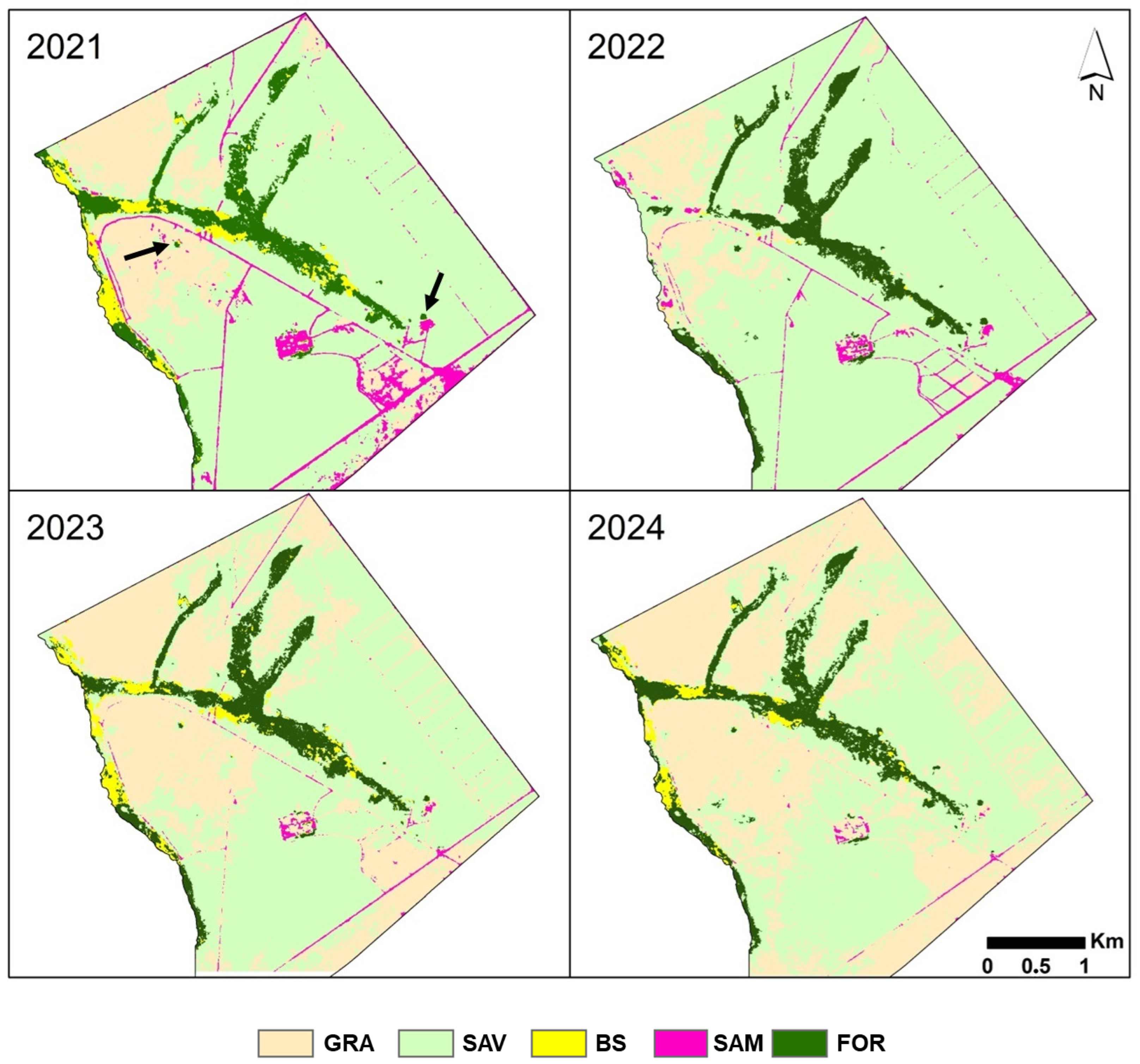
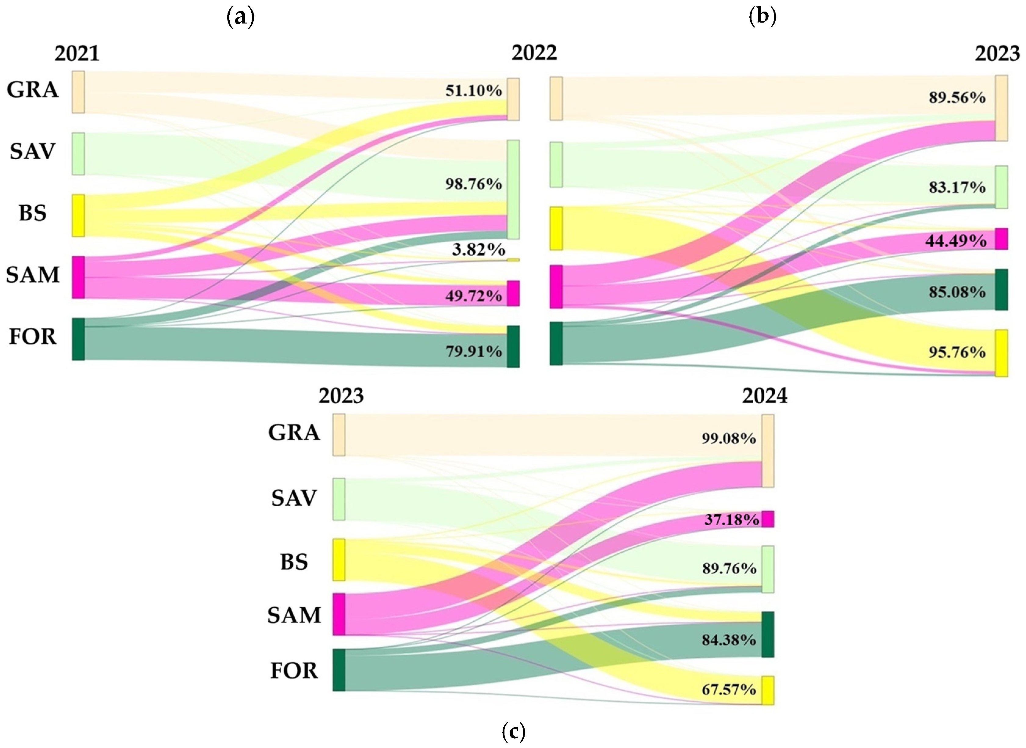
3.5. Land Cover from 2021 to 2024
4. Discussion
4.1. Cerrado Vegetation Mapping
4.2. Dynamic of Vegetation Formations from 2021 to 2024
5. Conclusions
Author Contributions
Funding
Data Availability Statement
Acknowledgments
Conflicts of Interest
References
- Mittermeier, R.A.; Myers, N.; Mittermeier, C.G.; Robles Gil, P. (Eds.) Hotspots: Earth’s Biologically Riches and Most Endangered Terrestrial Ecoregions, 1st ed.; CEMEX, Conservation International: Mexico City, Mexico, 1999; ISBN 978-968-6397-58-1. [Google Scholar]
- Silva, J.M.C.; Bates, J.M. Biogeographic Patterns and Conservation in the South American Cerrado: A Tropical Savanna Hotspot. BioScience 2002, 52, 225. [Google Scholar] [CrossRef]
- Klink, C.A.; Machado, R.B. Conservation of the Brazilian Cerrado. Conserv. Biol. 2005, 19, 707–713. [Google Scholar] [CrossRef]
- Alencar, A.; Shimbo, J.Z.; Lenti, F.; Balzani Marques, C.; Zimbres, B.; Rosa, M.; Arruda, V.; Castro, I.; Fernandes Márcico Ribeiro, J.; Varela, V.; et al. Mapping Three Decades of Changes in the Brazilian Savanna Native Vegetation Using Landsat Data Processed in the Google Earth Engine Platform. Remote Sens. 2020, 12, 924. [Google Scholar] [CrossRef]
- Klink, C.A.; Moreira, A.G. Past and Current Human Occupation, and Land Use. In The Cerrados of Brazil: Ecology and Natural History of a Neotropical Savanna; Columbia University Press: New York, NY, USA, 2002; pp. 69–88. [Google Scholar]
- Ribeiro, J.F.; Walter, B.M.T. Fitofisionomias do bioma Cerrado. In Cerrado: Ambiente e Flora; Sano, S.M., Almeida, S.P., Eds.; Embrapa-CPAC: Planaltina, DF, Brazil, 1998; Cap. 3; pp. 87–166. [Google Scholar]
- Solbrig, O.T. The Diversity of the Savanna Ecosystm. In Biodiversity and Savanna Ecosystem Processes; Solbrig, O.T., Medina, E., Silva, J.F., Eds.; Ecological Studies; Springer: Berlin/Heidelberg, Germany, 1996; Volume 121, pp. 31–41. ISBN 978-3-642-78971-7. [Google Scholar]
- Neri, A.V.; Schaefer, C.E.G.R.; Souza, A.L.; Ferreira-Junior, W.G.; Meira-Neto, J.A.A. Pedology and Plant Physiognomies in the Cerrado, Brazil. An. Acad. Bras. Ciênc. 2013, 85, 87–102. [Google Scholar] [CrossRef]
- Neves, S.P.S.; Funch, R.; Conceição, A.A.; Miranda, L.A.P.; Funch, L.S. What Are the Most Important Factors Determining Different Vegetation Types in the Chapada Diamantina, Brazil? Braz. J. Biol. 2016, 76, 315–333. [Google Scholar] [CrossRef]
- Bueno, M.L.; Dexter, K.G.; Pennington, R.T.; Pontara, V.; Neves, D.M.; Ratter, J.A.; De Oliveira-Filho, A.T. The Environmental Triangle of the Cerrado Domain: Ecological Factors Driving Shifts in Tree Species Composition between Forests and Savannas. J. Ecol. 2018, 106, 2109–2120. [Google Scholar] [CrossRef]
- Lewis, K.; De Van Barros, F.; Cure, M.B.; Davies, C.A.; Furtado, M.N.; Hill, T.C.; Hirota, M.; Martins, D.L.; Mazzochini, G.G.; Mitchard, E.T.A.; et al. Mapping Native and Non-Native Vegetation in the Brazilian Cerrado Using Freely Available Satellite Products. Sci. Rep. 2022, 12, 1588. [Google Scholar] [CrossRef]
- Lehmann, C.E.R.; Anderson, T.M.; Sankaran, M.; Higgins, S.I.; Archibald, S.; Hoffmann, W.A.; Hanan, N.P.; Williams, R.J.; Fensham, R.J.; Felfili, J.; et al. Savanna Vegetation-Fire-Climate Relationships Differ Among Continents. Science 2014, 343, 548–552. [Google Scholar] [CrossRef]
- Pivello, V.R.; Shida, C.N.; Meirelles, S.T. Alien Grasses in Brazilian Savannas: A Threat to the Biodiversity. Biodivers. Conserv. 1999, 8, 1281–1294. [Google Scholar] [CrossRef]
- Miatto, R.C.; Silva, I.A.; Silva-Matos, D.M.; Marrs, R.H. Woody Vegetation Structure of Brazilian Cerrado Invaded by Pteridium arachnoideum (Kaulf.) Maxon (Dennstaedtiaceae). Flora Morphol. Distrib. Funct. Ecol. Plants 2011, 206, 757–762. [Google Scholar] [CrossRef]
- Pivello, V.R.; Vieira, M.V.; Grombone-Guaratini, M.T.; Matos, D.M.S. Thinking about Super-Dominant Populations of Native Species—Examples from Brazil. Perspect. Ecol. Conserv. 2018, 16, 74–82. [Google Scholar] [CrossRef]
- Mistry, J.; Berardi, A. Assessing Fire Potential in a Brazilian Savanna Nature Reserve. Biotropica 2005, 37, 439–451. [Google Scholar] [CrossRef]
- Hoffmann, W.A.; Lucatelli, V.M.P.C.; Silva, F.J.; Azeuedo, I.N.C.; Marinho, M.D.S.; Albuquerque, A.M.S.; Lopes, A.D.O.; Moreira, S.P. Impact of the Invasive Alien Grass Melinis minutiflora at the Savanna-forest Ecotone in the Brazilian Cerrado. Divers. Distrib. 2004, 10, 99–103. [Google Scholar] [CrossRef]
- Hoffmann, W.A.; Haridasan, M. The Invasive Grass, Melinis minutiflora, Inhibits Tree Regeneration in a Neotropical Savanna. Austral Ecol. 2008, 33, 29–36. [Google Scholar] [CrossRef]
- Miranda, H.S.; Bustamente, M.M.C.; Miranda, A.C. The fire factor. In The Cerrados of Brazil: Ecology and Natural History of a Neotropical Savanna; Oliveira, P.S., Marquis, R.J., Eds.; Columbia University Press: New York, NY, USA, 2002; pp. 51–68. [Google Scholar]
- Assis, G.B.; Pilon, N.A.L.; Siqueira, M.F.; Durigan, G. Effectiveness and Costs of Invasive Species Control Using Different Techniques to Restore Cerrado Grasslands. Restor. Ecol. 2021, 29, e13219. [Google Scholar] [CrossRef]
- Souza, C.M.; Shimbo, J.Z.; Rosa, M.R.; Parente, L.L.; Alencar, A.A.; Rudorff, B.F.T.; Hasenack, H.; Matsumoto, M.; Ferreira, L.G.; Souza-Filho, P.W.M.; et al. Reconstructing Three Decades of Land Use and Land Cover Changes in Brazilian Biomes with Landsat Archive and Earth Engine. Remote Sens. 2020, 12, 2735. [Google Scholar] [CrossRef]
- Françoso, R.D.; Brandão, R.; Nogueira, C.C.; Salmona, Y.B.; Machado, R.B.; Colli, G.R. Habitat Loss and the Effectiveness of Protected Areas in the Cerrado Biodiversity Hotspot. Nat. Conserv. 2015, 13, 35–40. [Google Scholar] [CrossRef]
- Sano, E.E.; Rosa, R.; Brito, J.L.S.; Ferreira, L.G. Land Cover Mapping of the Tropical Savanna Region in Brazil. Environ. Monit. Assess. 2010, 166, 113–124. [Google Scholar] [CrossRef]
- Fonseca, L.M.G.; Körting, T.S.; Bendini, H.D.N.; Girolamo-Neto, C.D.; Neves, A.K.; Soares, A.R.; Taquary, E.C.; Maretto, R.V. Pattern Recognition and Remote Sensing Techniques Applied to Land Use and Land Cover Mapping in the Brazilian Savannah. Pattern Recognit. Lett. 2021, 148, 54–60. [Google Scholar] [CrossRef]
- Haddad, I.; Galvão, L.S.; Breunig, F.M.; Dalagnol, R.; Bourscheidt, V.; Jacon, A.D. On the Combined Use of Phenological Metrics Derived from Different PlanetScope Vegetation Indices for Classifying Savannas in Brazil. Remote Sens. Appl. Soc. Environ. 2022, 26, 100764. [Google Scholar] [CrossRef]
- FIBGE—Fundação Instituto Brasileiro de Geografia e Estatística. Zoneamento Ambiental da Bacia do Córrego Taquara—Distrito Federal; Versão Preliminar: Rio de Janeiro, Brazil, 1995; Volume I.
- UNESCO. Subsídios ao Zoneamento da APA Gama-Cabeça de Veado e Reserva da Biosfera do Cerrado: Caracterização e Conflitos Socioambientais; UNESCO, MAB, Reserva da Biosfera do Cerrado: Brasília, Brazil, 2003. [Google Scholar]
- Simões, K.C.C.; Hay, J.D.V.; de Andrade, C.O.; de Carvalho, O.A., Jr.; Gomes, R.A.T. Distribuição de Cana-do-Reino (Arundo donax L.) no Distrito Federal; Biodiversidade Brasileira-BioBrasil: Vinhedo, Brazil, 2013; p. 2.
- Martins, C.R.; Hay, J.D.V.; Valls, J.F.; Leite, L.L.; Henriques, R.P.B. Study on alien gramineous of the Brasilia National Park, Federal District, Brazil. Nat. Conserv. 2007, 5, 93–100. [Google Scholar]
- D’antonio, C.M.; Vitouek, P.M. Biological invasions by exotics grasses, the grass/fire, and goal change. Annu. Rev. Ecol. Evol. Syst. 1992, 23, 63–87. [Google Scholar] [CrossRef]
- Oliveira, V.M.; Schwartsburd, P.B.; Brighenti, A.M.; D’oliveira, P.S.; Miranda, J.E.C. Plantas tóxicas em pastagens: Samambaia-do-campo (Pteridium esculentum subsp. Archnoideum (kaulf) Thomson, Família Dennstaedtiaceae). In Comunicado Técnico; EMBRAPA: Brasilia, Brazil, 2018. [Google Scholar]
- Norway’s International Climate and Forests Initiative (NICFI). NICFI Satellite Data Program User Guide; Norway’s International Climate and Forests Initiative (NICFI): Oslo, Norway, 2022. [Google Scholar]
- Bueno, I.T.; Acerbi Júnior, F.W.; Silveira, E.M.O.; Mello, J.M.; Carvalho, L.M.T.; Gomide, L.R.; Withey, K.; Scolforo, J.R.S. Object-Based Change Detection in the Cerrado Biome Using Landsat Time Series. Remote Sens. 2019, 11, 570. [Google Scholar] [CrossRef]
- Breiman, L. Random Forests. Mach. Learn. 2001, 45, 5–32. [Google Scholar] [CrossRef]
- Sheykhmousa, M.; Mahdianpari, M.; Ghanbari, H.; Mohammadimanesh, F.; Ghamisi, P.; Homayouni, S. Support vector machine versus random forest for remote sensing image classification: A meta-analysis and systematic review. IEEE J. Sel. Top. Appl. Earth Obs. Remote Sens. 2020, 13, 6308–6325. [Google Scholar] [CrossRef]
- Jafarzadeh, H.; Mahdianpari, M.; Gill, E.; Mohammadimanesh, F.; Homayouni, S. Bagging and Boosting Ensemble Classifiers for Classification of Multispectral, Hyperspectral and PolSAR Data: A Comparative Evaluation. Remote Sens. 2021, 13, 4405. [Google Scholar] [CrossRef]
- Breiman, L. Using Adaptive Bagging to Debias Regressions; Technical Report 547; Statistics Dept, UCB: Brussels, Belgium, 1999. [Google Scholar]
- Chen, T.; Guestrin, C. XGBoost: A Scalable Tree Boosting System. In Proceedings of the 22nd ACM SIGKDD International Conference on Knowledge Discovery and Data Mining, San Francisco, CA, USA, 13 August 2016; ACM: New York, NY, USA, 2016; pp. 785–794. [Google Scholar]
- Friedman, J.H. Greedy function approximation: A gradient boosting machine. Ann. Stat. 2001, 29, 1189–1232. [Google Scholar] [CrossRef]
- Chemura, A.; Rwasoka, D.; Mutanga, O.; Dube, T.; Mushore, T. The Impact of Land-Use/Land Cover Changes on Water Balance of the Heterogeneous Buzi Sub-Catchment, Zimbabwe. Remote Sens. Appl. Soc. Environ. 2020, 18, 100292. [Google Scholar] [CrossRef]
- Vapnik, V.N. The Nature of Statistical Learning Theory, 2nd ed.; Springer: New York, NY, USA, 1995; p. 314. [Google Scholar]
- Kavzoglu, T.; Colkesen, I. A Kernel Functions Analysis for Support Vector Machines for Land Cover Classification. Int. J. Appl. Earth Obs. Geoinf. 2009, 11, 352–359. [Google Scholar] [CrossRef]
- Huang, C.; Davis, L.S.; Townshend, J.R.G. An Assessment of Support Vector Machines for Land Cover Classification. Int. J. Remote Sens. 2002, 23, 725–749. [Google Scholar] [CrossRef]
- Pouteau, R.; Meyer, J.-Y.; Taputuarai, R.; Stoll, B. Support Vector Machines to Map Rare and Endangered Native Plants in Pacific Islands Forests. Ecol. Inform. 2012, 9, 37–46. [Google Scholar] [CrossRef]
- Kulkarni, K.; Vijaya, P.A. Separability analysis of the band combinations for land cover classification of satellite images. Int. J. Eng. Trends Technol. 2021, 69, 138–144. [Google Scholar] [CrossRef]
- Souza, C.M.; Roberts, D.A.; Cochrane, M.A. Combining Spectral and Spatial Information to Map Canopy Damage from Selective Logging and Forest Fires. Remote Sens. Environ. 2005, 98, 329–343. [Google Scholar] [CrossRef]
- Congalton, R.G. A review of assessing the accuracy of classifications of remotely sensed data. Remote Sens. Environ. 1991, 37, 35–46. [Google Scholar] [CrossRef]
- Sasaki, Y. The truth of the F-measure. Teach. Tutor Mater. 2007, 1, 1–5. [Google Scholar]
- Cuba, N. Research Note: Sankey Diagrams for Visualizing Land Cover Dynamics. Landsc. Urban Plan. 2015, 139, 163–167. [Google Scholar] [CrossRef]
- Buja, A.; Swayne, D.F.; Littman, M.L.; Dean, N.; Hofmann, H.; Chen, L. Data Visualization with Multidimensional Scaling. J. Comput. Graph. Stat. 2008, 17, 444–472. [Google Scholar] [CrossRef]
- Guzmán, D.M.; Drummond, S.A.; Barreto, J.G. Undesirable Neighbours: Eucalyptus and Protected Areas. In Protected Area Management—Recent Advances; Nazip Suratman, M., Ed.; IntechOpen: London, UK, 2022; ISBN 978-1-83969-812-5. [Google Scholar]
- Liu, X.; Fu, D.; Zevenbergen, C.; Busker, T.; Yu, M. Assessing Sponge Cities Performance at City Scale Using Remotely Sensed LULC Changes: Case Study Nanjing. Remote Sens. 2021, 13, 580. [Google Scholar] [CrossRef]
- Acharki, S. PlanetScope contributions compared to Sentinel-2, and Landsat-8 for LULC mapping. Remote Sens. Appl. Soc. Environ. 2022, 27, 100774. [Google Scholar] [CrossRef]
- Schwieder, M.; Leitão, P.J.; Da Cunha Bustamante, M.M.; Ferreira, L.G.; Rabe, A.; Hostert, P. Mapping Brazilian Savanna Vegetation Gradients with Landsat Time Series. Int. J. Appl. Earth Obs. Geoinf. 2016, 52, 361–370. [Google Scholar] [CrossRef]
- Basheer, S.; Wang, X.; Farooque, A.A.; Nawaz, R.A.; Liu, K.; Adekanmbi, T.; Liu, S. Comparison of Land Use Land Cover Classifiers Using Different Satellite Imagery and Machine Learning Techniques. Remote Sens. 2022, 14, 4978. [Google Scholar] [CrossRef]
- Chachondhia, P.; Shakya, A.; Kumar, G. Performance Evaluation of Machine Learning Algorithms Using Optical and Microwave Data for LULC Classification. Remote Sens. Appl. Soc. Environ. 2021, 23, 100599. [Google Scholar] [CrossRef]
- Sheykhmousa, M.; Kerle, N.; Kuffer, M.; Ghaffarian, S. Post-Disaster Recovery Assessment with Machine Learning-Derived Land Cover and Land Use Information. Remote Sens. 2019, 11, 1174. [Google Scholar] [CrossRef]
- Camargo, F.F.; Sano, E.E.; Almeida, C.M.; Mura, J.C.; Almeida, T. A Comparative Assessment of Machine-Learning Techniques for Land Use and Land Cover Classification of the Brazilian Tropical Savanna Using ALOS-2/PALSAR-2 Polarimetric Images. Remote Sens. 2019, 11, 1600. [Google Scholar] [CrossRef]
- Zhang, P.; Ke, Y.; Zhang, Z.; Wang, M.; Li, P.; Zhang, S. Urban Land Use and Land Cover Classification Using Novel Deep Learning Models Based on High Spatial Resolution Satellite Imagery. Sensors 2018, 18, 3717. [Google Scholar] [CrossRef]
- Angelita, C.; Betânia, G.; Ionaí, M.; Mariza, P.; Leonardo, B. Frost Damage in a Lobelia Brasiliensis (Campanulaceae) Population at Reserva Ecologica Do Ibge, Brasilia –Federal District, Brazil. Rev. Biol. Neotrop. J. Neotrop. Biol. 2023, 20, 44–49. [Google Scholar]
- Brando, P.M.; Durigan, G. Changes in Cerrado Vegetation after Disturbance by Frost (São Paulo State, Brazil). Plant Ecol. 2004, 175, 205–215. [Google Scholar] [CrossRef]
- Miranda, H.S.; Sato, M.N.; Neto, W.N.; Aires, F.S. Fires in the Cerrado, the Brazilian Savanna. In Tropical Fire Ecology; Springer: Berlin/Heidelberg, Germany, 2009; pp. 427–450. ISBN 978-3-540-77380-1. [Google Scholar]
- Tambosi, L.R.; Barbosa, E.G. Uso de modelos de nicho ecológico, gerados em escala local, para identificação de áreas suscetíveis à invasão de gramíneas africanas em uma reserva de cerrado do estado de São Paulo. In Proceedings of the Anias XIV Simpósio Brasileiro de Sensoriamento Remoto, Natal, Brazil, 25–30 April 2009; INPE: Natal, Brazil, 2009; pp. 3111–3118. [Google Scholar]
- Sciamarelli, A.; Guglieri-Caporal, A.; Caporal, F.J.M. Prediction for expansion of two invasive grasses in Mato Grosso do Sul, Brazil, using climatic data and NDVI/MODIS. Número Espec. 2011, 36, 98–106. [Google Scholar]
- Hojo-Souza, N.S.; Carneiro, C.M.; Santos, R.C.d. Pteridium aquilinum: O que sabemos e o que ainda falta saber. Biosci. J. 2010, 26, 798–808. [Google Scholar]
- Zalba, S.M.; Cuevas, Y.A.; Boó, R.M. Invasion of Pinus halepensis Mill. following a wildfire in an Argentine grassland nature reserve. J. Environ. Manag. 2008, 88, 539–546. [Google Scholar] [CrossRef]
- Chen, C.R.; Condron, L.M.; Xu, Z.H. Impacts of grassland afforestation with coniferous trees on soil phosphorus dynamics and associated microbial processes: A review. For. Ecol. Manag. 2008, 255, 396–409. [Google Scholar] [CrossRef]
- Rejmanék, M.; Richardson, D.M. What attributes make some plant species more invasive? Ecology 1996, 77, 1655–1661. [Google Scholar] [CrossRef]
- Zanchetta, D.; Diniz, F.V. Estudo da contaminação biológica por Pinus spp. em três diferentes áreas na estação ecológica de Itirapina (SP, BRASIL). Rev. Inst. Florest. 2006, 18, 1–14. [Google Scholar] [CrossRef]


| Algorithm | Parameter | Values |
|---|---|---|
| RF | n_estimators | 100, 300, 500 |
| max_depth | 10, 20, 30 | |
| min_samples_split | 2, 5, 10 | |
| XGBoost | n_estimators | 100, 300, 500, 700 |
| max_depth | 3, 5, 7, 9 | |
| learning_rate | 0.01, 0.1, 0.2, 0,3 | |
| SVM | C | 0.1, 1, 10 |
| kernel | linear, poly, rbf | |
| degree | 2, 3, 4 | |
| gamma | scale, auto |
| Class Name | GRA | SAV | BS | SAM | FOR | Total | UA |
|---|---|---|---|---|---|---|---|
| GRA | 2061 | 0 | 36 | 0 | 0 | 2097 | 0.98 |
| SAV | 166 | 3994 | 4 | 0 | 2 | 4166 | 0.96 |
| BS | 0 | 2 | 499 | 0 | 0 | 501 | 1.00 |
| SAM | 0 | 9 | 0 | 555 | 11 | 575 | 0.97 |
| FOR | 0 | 24 | 0 | 11 | 2682 | 2717 | 0.99 |
| Total | 2227 | 4029 | 539 | 566 | 2695 | 10,056 | |
| PA | 0.93 | 0.99 | 0.93 | 0.98 | 1.00 |
| Class Name | GRA | SAV | BS | SAM | FOR | Total | UA |
|---|---|---|---|---|---|---|---|
| GRA | 2057 | 1 | 39 | 0 | 0 | 2097 | 0.98 |
| SAV | 169 | 3986 | 4 | 0 | 7 | 4166 | 0.96 |
| BS | 0 | 1 | 500 | 0 | 0 | 501 | 1.00 |
| SAM | 0 | 9 | 0 | 558 | 8 | 575 | 0.97 |
| FOR | 0 | 25 | 0 | 16 | 2676 | 2717 | 0.98 |
| Total | 2226 | 4022 | 543 | 574 | 2691 | 10,056 | |
| PA | 0.92 | 0.99 | 0.92 | 0.97 | 0.99 |
| Class Name | GRA | SAV | BS | SAM | FOR | Total | UA |
|---|---|---|---|---|---|---|---|
| GRA | 2093 | 0 | 4 | 0 | 0 | 2097 | 1.00 |
| SAV | 183 | 3983 | 0 | 0 | 0 | 4166 | 0.96 |
| BS | 0 | 5 | 496 | 0 | 0 | 501 | 0.99 |
| SAM | 0 | 9 | 0 | 558 | 8 | 575 | 0.97 |
| FOR | 0 | 29 | 0 | 12 | 2676 | 2717 | 0.98 |
| Total | 2276 | 4026 | 500 | 570 | 2684 | 10,056 | |
| PA | 0.92 | 0.99 | 0.99 | 0.98 | 1.00 |
| Algorithm | F1-Score (Weighted Avg) | OA (%) | kappa |
|---|---|---|---|
| RF | 0.97 | 97.3648 | 0.9629 |
| XGBoost | 0.97 | 97.2255 | 0.9609 |
| SVM | 0.98 | 97.5139 | 0.9649 |
| Comparison | Z | p-Value |
|---|---|---|
| RF vs. XGBoost: | 0.6204 | 0.5350 |
| RF vs. SVM | −0.6369 | 0.5242 |
| XGBoost vs. SVM | 1.2576 | 0.2086 |
Disclaimer/Publisher’s Note: The statements, opinions and data contained in all publications are solely those of the individual author(s) and contributor(s) and not of MDPI and/or the editor(s). MDPI and/or the editor(s) disclaim responsibility for any injury to people or property resulting from any ideas, methods, instructions or products referred to in the content. |
© 2025 by the authors. Licensee MDPI, Basel, Switzerland. This article is an open access article distributed under the terms and conditions of the Creative Commons Attribution (CC BY) license (https://creativecommons.org/licenses/by/4.0/).
Share and Cite
Rodrigues, T.; Takahashi, F.; Dias, A.; Lima, T.; Alcântara, E. Machine Learning-Based Cerrado Land Cover Classification Using PlanetScope Imagery. Remote Sens. 2025, 17, 480. https://doi.org/10.3390/rs17030480
Rodrigues T, Takahashi F, Dias A, Lima T, Alcântara E. Machine Learning-Based Cerrado Land Cover Classification Using PlanetScope Imagery. Remote Sensing. 2025; 17(3):480. https://doi.org/10.3390/rs17030480
Chicago/Turabian StyleRodrigues, Thanan, Frederico Takahashi, Arthur Dias, Taline Lima, and Enner Alcântara. 2025. "Machine Learning-Based Cerrado Land Cover Classification Using PlanetScope Imagery" Remote Sensing 17, no. 3: 480. https://doi.org/10.3390/rs17030480
APA StyleRodrigues, T., Takahashi, F., Dias, A., Lima, T., & Alcântara, E. (2025). Machine Learning-Based Cerrado Land Cover Classification Using PlanetScope Imagery. Remote Sensing, 17(3), 480. https://doi.org/10.3390/rs17030480