
SDGSAT-1 Cloud Detection Algorithm Based on RDE-SegNeXt


Abstract
1. Introduction
- 1.
- We have refined the labeling and constructed a new SDGSAT-1 cloud detection dataset. The dataset consists of 15,000 finely labeled feature classes, including clouds, cloud shadow, snow, water and land, required for the five SDGSAT missions, in order to address the lack of data in the field of SDGSAT cloud detection and to promote the subsequent application and dissemination of the data.
- 2.
- We propose a new convolutional attention module, called RDE-MSCA (re-parameterized detail-enhanced multi-scale convolutional attention), which on the one hand can establish the parameter link between different channels of convolutional kernels through re-parameterization, and on the other hand can reduce the computational complexity, Finally, the gated linear structure enables the model to adaptively weight the detail-enhanced convolution information to improve the expressiveness of the network, so as to make full use of the feature information and computational resources to improve the accuracy of cloud detection. information and computational resources to improve the accuracy and efficiency of cloud detection.
- 3.
- Based on the RDE-MSCA module, we propose a re-parameterized convolutional attention network with detail-enhanced convolution RDE-SegNeXt for the cloud detection task of SDGSAT-1 data, and experimentally demonstrate the model’s excellent ability to discriminate and detect clouds and cloud shadow, and clouds and snow of SDGSAT-1 data, while ensuring low computational complexity and high inference speed. In addition, we also demonstrate its excellent performance for other cloud detection tasks on the public cloud detection dataset 38-Cloud, and further demonstrate the competitive detection accuracy of RDE-SegNeXt on the public remote sensing dataset LoveDA for the detection of other remote sensing data features, demonstrating the universal applicability and effectiveness of the model.
2. Materials and Methods
2.1. SDGSAT-1
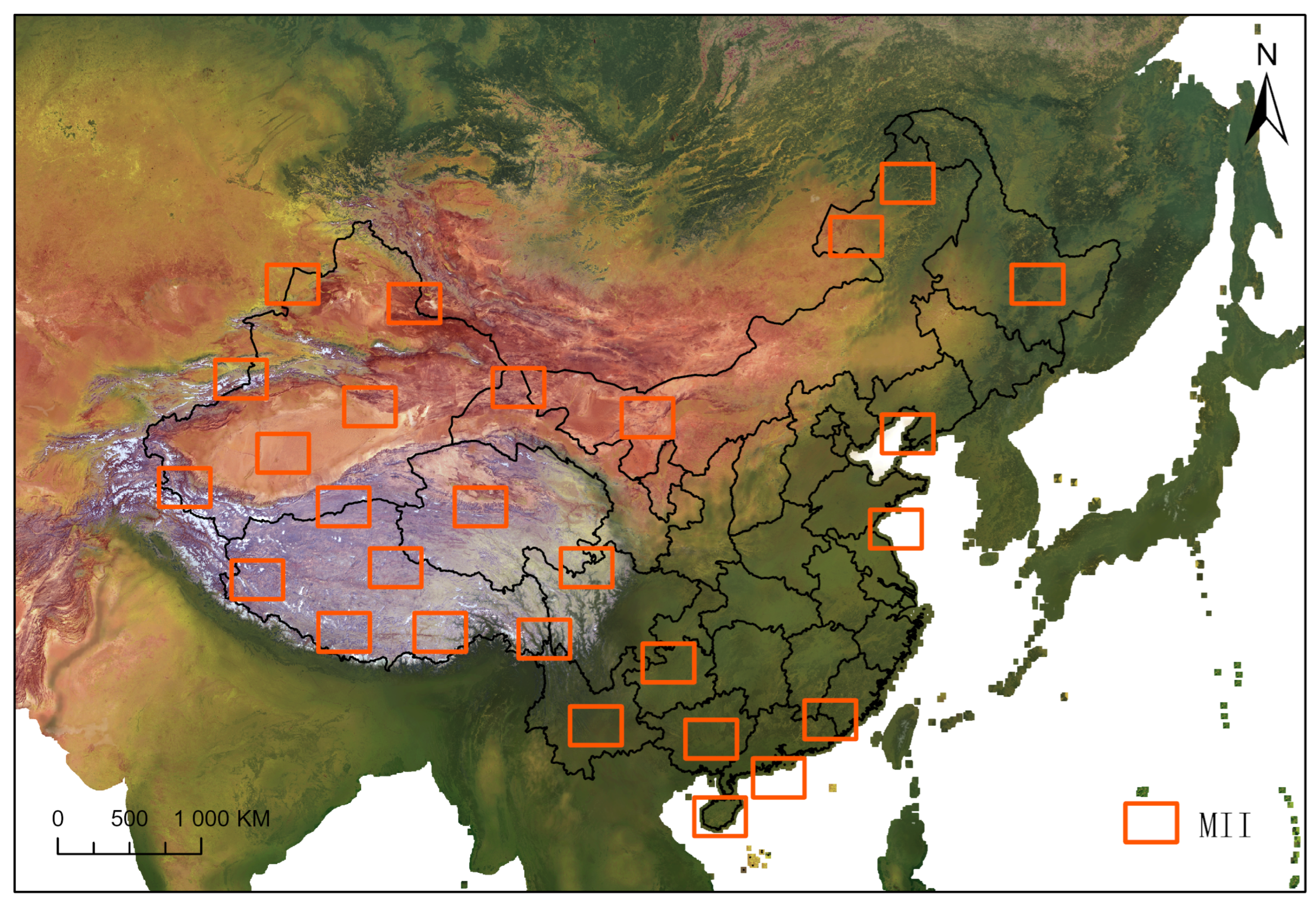
2.1.1. Areas
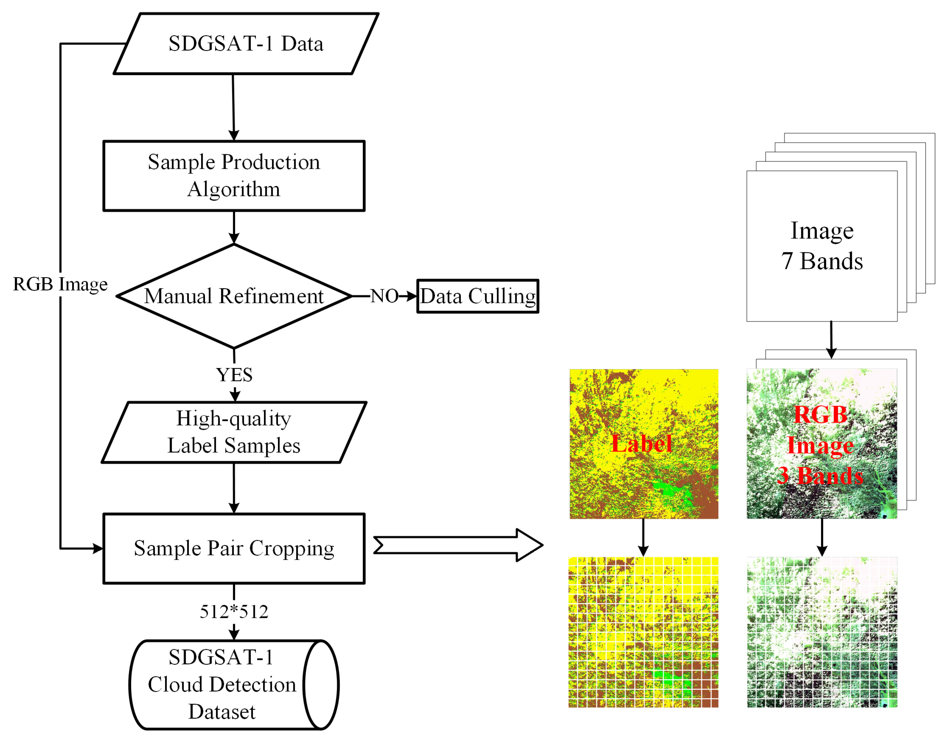
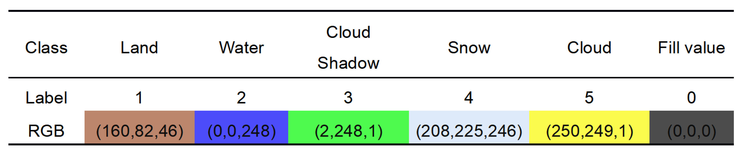
2.1.2. Sample Production and Labeling Process
- (1)
- Threshold method to automatically generate initial tags
- (2)
- Manual Refinement
- (3)
- Sample Pair Cropping
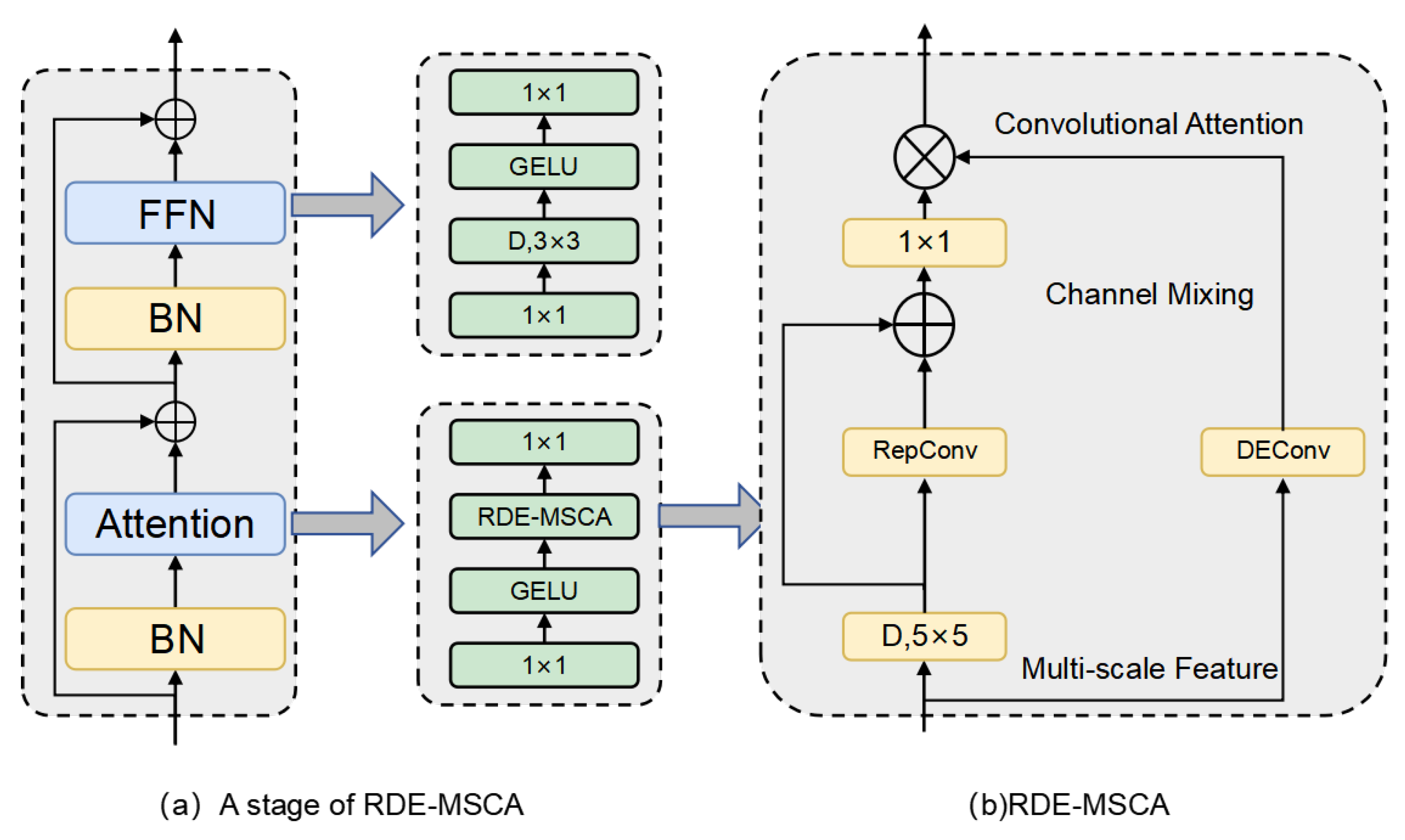
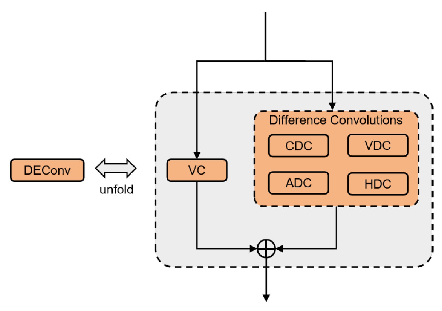
2.2. RDE-MSCA
- (1)
- Vanilla convolution: extracts the intensity level information of the image, i.e., traditional convolution operation.
- (2)
- Centre difference convolution: Calculates the centre difference of each pixel in the image, captures the difference between the centre pixel and its surrounding neighborhood, and is used to capture fine-grained gradient information. CDC modifies the convolution weights so that the centre weight is subtracted from the sum of the surrounding weights, and enhances sensitivity to edges during feature extraction by emphasizing the contrast between the centre and the surroundings.
- (3)
- Angular difference convolution: Extracts the gradient information of each angle in the image to effectively capture the corner features and angular differences in the image, which is very useful for detecting corner-like structures. The ADC adjusts the weights to compute the differences in the angular direction and introduces the parameter theta to control the degree of angular differences.
- (4)
- Horizontal difference convolution: calculates the difference in the horizontal direction and is used to enhance horizontal edge features.
- (5)
- Vertical difference convolution: computes the difference in the vertical direction and is used to enhance vertical edge features.
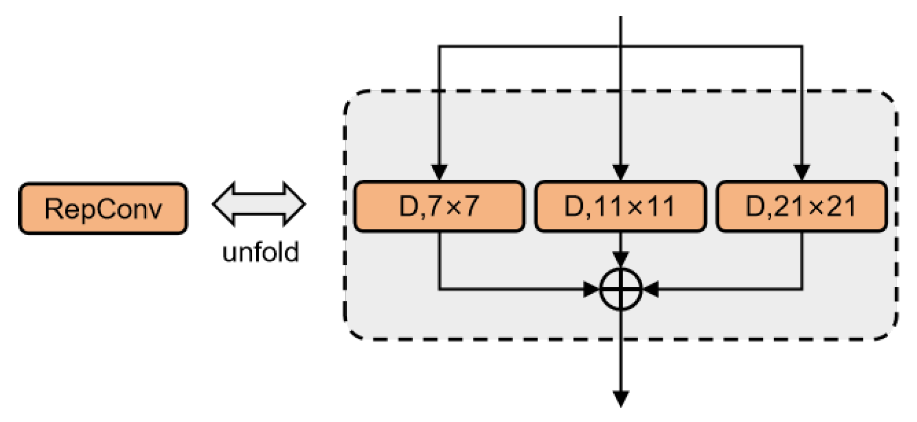
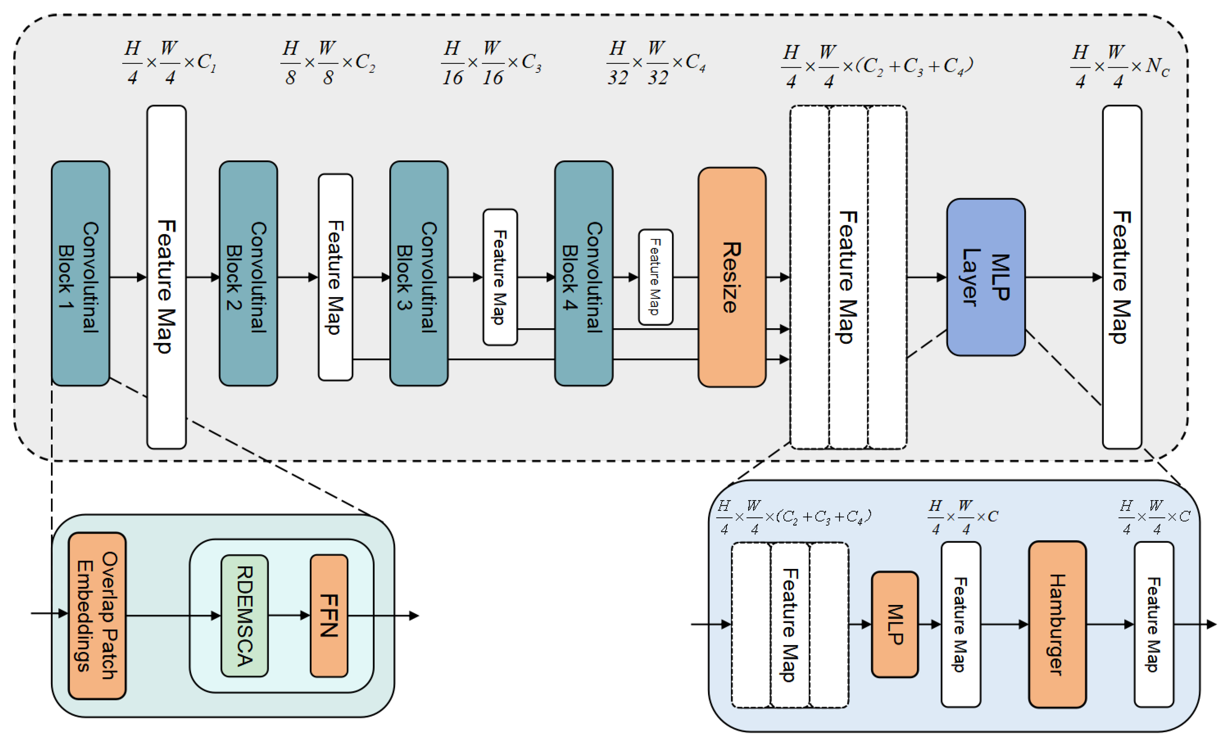
2.3. RDE-SegNeXt
3. Experiments
3.1. Datasets and Evaluation Metrics
3.1.1. Datasets
3.1.2. Evaluation Metrics
3.2. Implementation Details
3.3. Ablation Study
3.4. Comparison Experiments
3.4.1. Comparative Experiments of the SDGSAT-1 Dataset
- I.
- Quantitative Analysis
- II.
- Efficiency analysis
- III.
- Qualitative analysis
3.4.2. 38-Cloud Public Cloud Dataset Comparison Experiments
- I.
- Quantitative analysis
- II.
- Quantitative analysis
3.4.3. LoveDA Public Dataset Comparison Experiments
- I.
- Quantitative analysis
- (a)
- Overall performance analysisAs shown in the Table 9, RDE-SegNeXt achieved the highest overall performance with mFscore (64.68%), aAcc (64.68%), mIoU (48.51%) and mAcc (61.33%). This is a 1.84% improvement in mIoU and a 1.9% improvement in mFscore over the previous top performer, PoolFormer (46.67% mIoU, 62.78% mFscore). Compared with the Swin Transformer series, which also has high accuracy, RDE-SegNeXt not only has a 6%–8% improvement in mIoU (e.g., 42.44% for Swin-L compared to 48.51% for RDE-SegNeXt), but also improves the F1 scores by about 5.77%, which demonstrates a better comprehensive segmentation capability and global accuracy.
- (b)
- Category analysisAccording to the IoU and Acc metrics of each category in the Table 10, RDE-SegNeXt achieves the best or near-best performance in most of the categories, which demonstrates its excellent adaptability to the composite urban and natural scenes. For the roads category RDE-SegNeXt achieves the highest IoU (52.20%) in the roads category, thanks to the effective capture of edges and fine structures by the detail-enhanced convolution, especially for narrow and continuous road targets. For bare ground and agricultural land, RDE-SegNeXt also achieves the best performance on the bare ground and agricultural land categories, indicating the model’s strength in recognizing complex features such as sparsely vegetated areas and agricultural land. For the buildings and forests categories: the RDE-SegNeXt also performs well on the buildings and forests categories, showing the advantage of RepConv in capturing large-scale shapes and local textures with the DEConv parallel branch.
- II.
- Qualitative Analysis
4. Discussion
5. Conclusions
Author Contributions
Funding
Data Availability Statement
Acknowledgments
Conflicts of Interest
References
- King, M.D.; Platnick, S.; Menzel, W.P.; Ackerman, S.A.; Hubanks, P.A. Spatial and temporal distribution of clouds observed by MODIS onboard the Terra and Aqua satellites. IEEE Trans. Geosci. Remote Sens. 2013, 51, 3826–3852. [Google Scholar] [CrossRef]
- Meng, X.; Shen, H.; Yuan, Q.; Li, H.; Zhang, L.; Sun, W. Pansharpening for cloud-contaminated very high-resolution remote sensing images. IEEE Trans. Geosci. Remote Sens. 2018, 57, 2840–2854. [Google Scholar] [CrossRef]
- Shen, H.; Wu, J.; Cheng, Q.; Aihemaiti, M.; Zhang, C.; Li, Z. A spatiotemporal fusion based cloud removal method for remote sensing images with land cover changes. IEEE J. Sel. Top. Appl. Earth Obs. Remote Sens. 2019, 12, 862–874. [Google Scholar] [CrossRef]
- Zou, Z.; Shi, Z. Ship detection in spaceborne optical image with SVD networks. IEEE Trans. Geosci. Remote Sens. 2016, 54, 5832–5845. [Google Scholar] [CrossRef]
- Ma, A.; Wang, J.; Zhong, Y.; Zheng, Z. FactSeg: Foreground activation-driven small object semantic segmentation in large-scale remote sensing imagery. IEEE Trans. Geosci. Remote Sens. 2021, 60, 5606216. [Google Scholar] [CrossRef]
- Chen, H.; Li, W.; Shi, Z. Adversarial instance augmentation for building change detection in remote sensing images. IEEE Trans. Geosci. Remote Sens. 2021, 60, 5603216. [Google Scholar] [CrossRef]
- Guo, H.; Dou, C.; Chen, H.; Liu, J.; Fu, B.; Li, X.; Zou, Z.; Liang, D. SDGSAT-1: The world’s first scientific satellite for sustainable development goals. Sci. Bull. 2023, 68, 34–38. [Google Scholar] [CrossRef]
- Irish, R.R.; Barker, J.L.; Goward, S.N.; Arvidson, T. Characterization of the Landsat-7 ETM+ automated cloud-cover assessment (ACCA) algorithm. Photogramm. Eng. Remote Sens. 2006, 72, 1179–1188. [Google Scholar] [CrossRef]
- Zhu, Z.; Woodcock, C.E. Object-based cloud and cloud shadow detection in Landsat imagery. Remote Sens. Environ. 2012, 118, 83–94. [Google Scholar] [CrossRef]
- Luo, Y.; Trishchenko, A.P.; Khlopenkov, K.V. Developing clear-sky, cloud and cloud shadow mask for producing clear-sky composites at 250-meter spatial resolution for the seven MODIS land bands over Canada and North America. Remote Sens. Environ. 2008, 112, 4167–4185. [Google Scholar] [CrossRef]
- Liu, X.; Xu, J.; Du, B. Automatic Cloud Detection of GMS-5 Images with Dual-Channel Dynamic Thresholding. J. Appl. Meteorol. 2005, 16, 434–444. [Google Scholar]
- Ma, F.; Zhang, Q.; Guo, N.; Zhang, J. Research on cloud detection methods for multi-channel satellite cloud maps. Atmos. Sci. 2007, 31, 119–128. [Google Scholar]
- Zhu, Z.; Wang, S.; Woodcock, C.E. Improvement and expansion of the Fmask algorithm: Cloud, cloud shadow, and snow detection for Landsats 4–7, 8, and Sentinel 2 images. Remote Sens. Environ. 2015, 159, 269–277. [Google Scholar] [CrossRef]
- Dong, Z.; Sun, L.; Liu, X.; Wang, Y.; Liang, T. CDAG-Improved Algorithm and Its Application to GF-6 WFV Data Cloud Detection. Acta Opt. Sin 2020, 40, 143–152. [Google Scholar]
- Sun, L.; Mi, X.; Wei, J.; Wang, J.; Tian, X.; Yu, H.; Gan, P. A cloud detection algorithm-generating method for remote sensing data at visible to short-wave infrared wavelengths. ISPRS J. Photogramm. Remote Sens. 2017, 124, 70–88. [Google Scholar] [CrossRef]
- Mi, W.; Zhiqi, Z.; Zhipeng, D.; Shuying, J.; SU, H. Stream-computing based high accuracy on-board real-time cloud detection for high resolution optical satellite imagery. Acta Geod. Cartogr. Sin. 2018, 47, 760. [Google Scholar]
- Changmiao, H.; Zheng, Z.; Ping, T. Research on multispectral satellite image cloud and cloud shadow detection algorithm of domestic satellite. Natl. Remote Sens. Bull. 2023, 27, 623–634. [Google Scholar]
- Ge, K.; Liu, J.; Wang, F.; Chen, B.; Hu, Y. A Cloud Detection Method Based on Spectral and Gradient Features for SDGSAT-1 Multispectral Images. Remote Sens. 2022, 15, 24. [Google Scholar] [CrossRef]
- Xie, Y.; Ma, C.; Wan, G.; Chen, H.; Fu, B. Cloud detection using SDGSAT-1 thermal infrared data. In Proceedings of the Remote Sensing of Clouds and the Atmosphere XXVIII. SPIE, Amsterdam, The Netherland, 5–6 September 2023; Volume 12730, pp. 77–82. [Google Scholar]
- Jiao, L.; Huo, L.; Hu, C.; Tang, P. Refined UNet v3: Efficient end-to-end patch-wise network for cloud and shadow segmentation with multi-channel spectral features. Neural Networks 2021, 143, 767–782. [Google Scholar] [CrossRef] [PubMed]
- Li, Z.; Shen, H.; Cheng, Q.; Liu, Y.; You, S.; He, Z. Deep learning based cloud detection for medium and high resolution remote sensing images of different sensors. ISPRS J. Photogramm. Remote Sens. 2019, 150, 197–212. [Google Scholar] [CrossRef]
- Shao, Z.; Pan, Y.; Diao, C.; Cai, J. Cloud detection in remote sensing images based on multiscale features-convolutional neural network. IEEE Trans. Geosci. Remote Sens. 2019, 57, 4062–4076. [Google Scholar] [CrossRef]
- Fan, X.; Chang, H.; Huo, L.; Hu, C. Gf-1/6 satellite pixel-by-pixel quality tagging algorithm. Remote Sens. 2023, 15, 1955. [Google Scholar] [CrossRef]
- Chang, H.; Fan, X.; Huo, L.; Hu, C. Improving Cloud Detection in WFV Images Onboard Chinese GF-1/6 Satellite. Remote Sens. 2023, 15, 5229. [Google Scholar] [CrossRef]
- Qin, X.; Wang, Z.; Bai, Y.; Xie, X.; Jia, H. FFA-Net: Feature fusion attention network for single image dehazing. In Proceedings of the AAAI Conference on Artificial Intelligence, New York, NY, USA, 7–12 February 2020; Volume 34, pp. 11908–11915. [Google Scholar]
- Wu, H.; Qu, Y.; Lin, S.; Zhou, J.; Qiao, R.; Zhang, Z.; Xie, Y.; Ma, L. Contrastive learning for compact single image dehazing. In Proceedings of the IEEE/CVF Conference on Computer Vision and Pattern Recognition, Nashville, TN, USA, 20–25 June 2021; pp. 10551–10560. [Google Scholar]
- Wu, H.; Liu, J.; Xie, Y.; Qu, Y.; Ma, L. Knowledge transfer dehazing network for nonhomogeneous dehazing. In Proceedings of the IEEE/CVF conference on Computer Vision and Pattern Recognition Workshops, Seattle, WA, USA, 14–19 June 2020; pp. 478–479. [Google Scholar]
- Zhang, H.; Patel, V.M. Densely connected pyramid dehazing network. In Proceedings of the IEEE Conference on Computer Vision and Pattern Recognition, Salt Lake City, UT, USA, 18–23 June 2018; pp. 3194–3203. [Google Scholar]
- Bai, H.; Pan, J.; Xiang, X.; Tang, J. Self-guided image dehazing using progressive feature fusion. IEEE Trans. Image Process. 2022, 31, 1217–1229. [Google Scholar] [CrossRef] [PubMed]
- Wang, C.; Shen, H.Z.; Fan, F.; Shao, M.W.; Yang, C.S.; Luo, J.C.; Deng, L.J. EAA-Net: A novel edge assisted attention network for single image dehazing. Knowl.-Based Syst. 2021, 228, 107279. [Google Scholar] [CrossRef]
- Cai, Z.; Ding, X.; Shen, Q.; Cao, X. Refconv: Re-parameterized refocusing convolution for powerful convnets. arXiv 2023, arXiv:2310.10563. [Google Scholar]
- Ding, X.; Zhang, X.; Ma, N.; Han, J.; Ding, G.; Sun, J. Repvgg: Making vgg-style convnets great again. In Proceedings of the IEEE/CVF Conference on Computer Vision and Pattern Recognition, Nashville, TN, USA, 20–15 June 2021; pp. 13733–13742. [Google Scholar]
- Dauphin, Y.N.; Fan, A.; Auli, M.; Grangier, D. Language modeling with gated convolutional networks. In Proceedings of the International Conference on Machine Learning, PMLR, Sydney, NSW, Australia, 6–11 August 2017; pp. 933–941. [Google Scholar]
- Shazeer, N. Glu variants improve transformer. arXiv 2020, arXiv:2002.05202. [Google Scholar]
- Narang, S.; Chung, H.W.; Tay, Y.; Fedus, W.; Fevry, T.; Matena, M.; Malkan, K.; Fiedel, N.; Shazeer, N.; Lan, Z.; et al. Do transformer modifications transfer across implementations and applications? arXiv 2021, arXiv:2102.11972. [Google Scholar]
- Hua, W.; Dai, Z.; Liu, H.; Le, Q. Transformer quality in linear time. In Proceedings of the International conference on machine learning, PMLR, Baltimore, MA, USA, 17–23 July 2022; pp. 9099–9117. [Google Scholar]
- Du, N.; Huang, Y.; Dai, A.M.; Tong, S.; Lepikhin, D.; Xu, Y.; Krikun, M.; Zhou, Y.; Yu, A.W.; Firat, O.; et al. Glam: Efficient scaling of language models with mixture-of-experts. In Proceedings of the International Conference on Machine Learning, PMLR, Baltimore, MA, USA, 17–23 July 2022; pp. 5547–5569. [Google Scholar]
- Thoppilan, R.; De Freitas, D.; Hall, J.; Shazeer, N.; Kulshreshtha, A.; Cheng, H.T.; Jin, A.; Bos, T.; Baker, L.; Du, Y.; et al. Lamda: Language models for dialog applications. arXiv 2022, arXiv:2201.08239. [Google Scholar]
- Hu, J.; Shen, L.; Sun, G. Squeeze-and-excitation networks. In Proceedings of the IEEE Conference on Computer Vision and Pattern Recognition, Salt Lake City, UT, USA, 18–28 June 2018; pp. 7132–7141. [Google Scholar]
- Woo, S.; Park, J.; Lee, J.Y.; Kweon, I.S. Cbam: Convolutional block attention module. In Proceedings of the European Conference on Computer Vision (ECCV), Munich, Germany, 8–14 September 2018; pp. 3–19. [Google Scholar]
- Wang, J.; Sun, K.; Cheng, T.; Jiang, B.; Deng, C.; Zhao, Y.; Liu, D.; Mu, Y.; Tan, M.; Wang, X.; et al. Deep high-resolution representation learning for visual recognition. IEEE Trans. Pattern Anal. Mach. Intell. 2020, 43, 3349–3364. [Google Scholar] [CrossRef]
- Chen, L.C. Rethinking atrous convolution for semantic image segmentation. arXiv 2017, arXiv:1706.05587. [Google Scholar]
- Cheng, B.; Misra, I.; Schwing, A.G.; Kirillov, A.; Girdhar, R. Masked-attention mask transformer for universal image segmentation. In Proceedings of the IEEE/CVF Conference on Computer Vision and Pattern Recognition, New Orleans, LA, USA, 18–24 June 2022; pp. 1290–1299. [Google Scholar]
- Yu, W.; Luo, M.; Zhou, P.; Si, C.; Zhou, Y.; Wang, X.; Feng, J.; Yan, S. Metaformer is actually what you need for vision. In Proceedings of the IEEE/CVF Conference on Computer Vision and Pattern Recognition, New Orleans, LA, USA, 18–24 June 2022; pp. 10819–10829. [Google Scholar]
- Wang, L.; Fang, S.; Meng, X.; Li, R. Building extraction with vision transformer. IEEE Trans. Geosci. Remote Sens. 2022, 60, 1–11. [Google Scholar] [CrossRef]
- Fu, J.; Liu, J.; Tian, H.; Li, Y.; Bao, Y.; Fang, Z.; Lu, H. Dual attention network for scene segmentation. In Proceedings of the IEEE/CVF Conference on Computer Vision and Pattern Recognition, Long Beach, CA, USA, 15–19 June 2019; pp. 3146–3154. [Google Scholar]
- Strudel, R.; Garcia, R.; Laptev, I.; Schmid, C. Segmenter: Transformer for Semantic Segmentation. In Proceedings of the IEEE/CVF international Conference on Computer Vision, Nashville, TN, USA, 20–25 June 2021; pp. 7262–7272. [Google Scholar]
- Yuan, W.; Wang, J.; Xu, W. Shift pooling PSPNet: Rethinking PSPNet for building extraction in remote sensing images from entire local feature pooling. Remote Sens. 2022, 14, 4889. [Google Scholar] [CrossRef]
- Liu, Z.; Mao, H.; Wu, C.Y.; Feichtenhofer, C.; Darrell, T.; Xie, S. A convnet for the 2020s. In Proceedings of the IEEE/CVF Conference on Computer Vision and Pattern Recognition, New Orleans, LA, USA, 18–24 June 2022; pp. 11976–11986. [Google Scholar]
- Liu, Z.; Lin, Y.; Cao, Y.; Hu, H.; Wei, Y.; Zhang, Z.; Lin, S.; Guo, B. Swin transformer: Hierarchical vision transformer using shifted windows. In Proceedings of the IEEE/CVF international Conference on Computer Vision, Montreal, QC, Canada, 10–17 October 2021; pp. 10012–10022. [Google Scholar]
- Guo, M.H.; Lu, C.Z.; Hou, Q.; Liu, Z.; Cheng, M.M.; Hu, S.M. Segnext: Rethinking convolutional attention design for semantic segmentation. Adv. Neural Inf. Process. Syst. 2022, 35, 1140–1156. [Google Scholar]
- Wang, J.; Zheng, Z.; Ma, A.; Lu, X.; Zhong, Y. LoveDA: A remote sensing land-cover dataset for domain adaptive semantic segmentation. arXiv 2021, arXiv:2110.08733. [Google Scholar]
- Cubuk, E.D.; Zoph, B.; Shlens, J.; Le, Q.V. Randaugment: Practical automated data augmentation with a reduced search space. In Proceedings of the IEEE/CVF Conference on Computer Vision and Pattern Recognition Workshops, Seattle, WA, USA, 14–19 June 2020; pp. 702–703. [Google Scholar]
- Liu, Z.; Hu, H.; Lin, Y.; Yao, Z.; Xie, Z.; Wei, Y.; Ning, J.; Cao, Y.; Zhang, Z.; Dong, L.; et al. Swin transformer v2: Scaling up capacity and resolution. In Proceedings of the IEEE/CVF Conference on Computer Vision and Pattern Recognition, New Orleans, LA, USA, 18–24 June 2022; pp. 12009–12019. [Google Scholar]


| Landsat-8 | Sentinel-2A | Sentinel-2B | GF-1 | GF-6 | SDGSAT-1 | |
|---|---|---|---|---|---|---|
| Coastal Blue | 0.433–0.453 | 0.432–0.453 | 0.432–0.453 | — | 0.40–0.45 | 0.37–0.427 0.41–0.467 |
| Blue | 0.450–0.515 | 0.459–0.525 | 0.459–0.525 | 0.45–0.52 | 0.45–0.52 | 0.457–0.529 |
| Green | 0.525–0.600 | 0.542–0.578 | 0.541–0.577 | 0.52–0.59 | 0.52–0.59 | 0.51-0.597 |
| Yellow | — | — | — | — | 0.59-0.63 | — |
| Red | 0.630–0.680 | 0.649–0.680 | 0.650–0.681 | 0.63–0.69 | 0.63–0.69 | 0.618–0.696 |
| Red Edge 1 Red Edge 2 Red Edge 3 | — | 0.697–0.712 0.733–0.748 0.773–0.793 | 0.696–0.712 0.732–0.747 0.770–0.790 | — | 0.69–0.73 0.73–0.77 | 0.744–0.813 |
| NIR Narrow NIR | 0.845–0.885 | 0.780–0.886 0.854–0.875 | 0.780–0.886 0.853–0.875 | 0.77–0.89 | 0.77–0.89 | 0.798–0.911 |
| Water vapor | — | 0.935–0.955 | 0.933–0.954 | — | — | — |
| Cirrus | 1.360–1.390 | 1.358–1.389 | 1.362–1.392 | — | — | — |
| SWIR 1 | 1.560–1.660 | 1.568–1.659 | 1.563–1.657 | — | — | — |
| SWIR 2 | 2.100–2.300 | 2.115–2.290 | 2.093–2.278 | — | — | — |
| TIRS 1 | 10.60–11.19 | — | — | — | — | — |
| TIRS 2 | 11.50–12.51 | — | — | — | — | — |
| Type | Item of Indicators | Specific Indicators |
|---|---|---|
| Orbit | Track Type | Solar synchronous orbit |
| Orbital Altitude | 505 km | |
| Orbital Inclination | ||
| MII | Image Width | 300 km |
| Detection Spectrum | B1: 374 nm∼427 nm | |
| B2: 410 nm∼467 nm | ||
| B3: 457 nm∼529 nm | ||
| B4: 510 nm∼597 nm | ||
| B5: 618 nm∼696 nm | ||
| B6: 744 nm∼813 nm | ||
| B7: 798 nm∼811 nm | ||
| Pixel Resolution | 10 m |
| Stage | Output Size | e.r. | Tiny | Small | Base | Large |
|---|---|---|---|---|---|---|
| 1 | 8 | C = 32 L = 3 | C = 64 L = 2 | C = 64 L = 3 | C = 64 L = 3 | |
| 2 | 8 | C=64 L = 3 | C = 128 L = 2 | C = 128 L = 3 | C = 128 L = 5 | |
| 3 | 4 | C = 160 L = 5 | C = 320 L = 4 | C = 320 L = 12 | C = 320 L = 27 | |
| 4 | 4 | C = 256 L = 2 | C = 512 L = 2 | C = 512 L = 3 | C = 512 L = 3 |
| Methods | mFscore | mIOU | mAcc |
|---|---|---|---|
| SegNext-Tiny | 77.33 | 66.59 | 74.24 |
| SegNext-Tiny+RepConv | 78.03 | 67.50 | 75.15 |
| SegNext-Tiny+DEConv | 79.19 | 68.89 | 77.16 |
| SegNext-Tiny+RepConv+DEConv (ALL) | 79.63 | 69.25 | 78.00 |
| SegNext-Tiny+RepConv+RepConv (First) | 75.21 | 66.95 | 77.78 |
| SegNext-Tiny+RepConv+DEConv (First) | 81.77 | 71.85 | 81.83 |
| Model | mFscore | aAcc | mIoU | mAcc |
|---|---|---|---|---|
| Hrnet [41] | 68.82 | 85.90 | 56.30 | 62.76 |
| Deeplabv3+ [42] | 67.07 | 84.32 | 54.42 | 65.31 |
| Mask2former [43] | 72.88 | 79.89 | 59.52 | 70.90 |
| PoolFormer [44] | 77.69 | 88.09 | 67.64 | 76.93 |
| BuildFormer [45] | 79.63 | 88.07 | 69.01 | 78.82 |
| DANet [46] | 73.34 | 85.26 | 62.58 | 70.39 |
| Segmenter [47] | 75.26 | 85.89 | 64.26 | 72.61 |
| SP-PSPNet [48] | 79.62 | 88.06 | 69.12 | 79.35 |
| ConvNeXt-T [49] | 72.53 | 84.69 | 61.02 | 68.92 |
| ConvNeXt-S [49] | 76.98 | 86.56 | 66.12 | 75.85 |
| ConvNeXt-B [49] | 78.55 | 87.17 | 67.98 | 77.06 |
| ConvNeXt-L [49] | 78.73 | 87.78 | 68.29 | 76.60 |
| Swin-T [50] | 77.57 | 87.47 | 66.61 | 73.74 |
| Swin-S [50] | 78.44 | 87.76 | 67.61 | 76.05 |
| Swin-B [50] | 78.74 | 87.07 | 67.40 | 75.47 |
| Swin-L [54] | 79.69 | 88.21 | 69.14 | 76.55 |
| SegNext-T [51] | 77.33 | 86.98 | 66.59 | 74.24 |
| SegNext-S [51] | 78.51 | 87.38 | 67.95 | 76.42 |
| SegNext-B [51] | 79.46 | 87.75 | 68.98 | 77.37 |
| SegNext-L [51] | 79.53 | 88.03 | 69.25 | 77.50 |
| RDE-SegNext | 81.77 | 89.03 | 71.85 | 81.83 |
| Model | Land (1) | Water (2) | Shadow (3) | Snow (4) | Cloud (5) | |||||
|---|---|---|---|---|---|---|---|---|---|---|
| IoU (%) | Acc (%) | IoU (%) | Acc (%) | IoU (%) | Acc (%) | IoU (%) | Acc (%) | IoU (%) | Acc (%) | |
| Hrnet | 80.8 | 95.31 | 30.76 | 31.44 | 25.38 | 28.76 | 63.19 | 68.47 | 81.37 | 89.83 |
| Deeplabv3+ | 75.22 | 87.96 | 25.83 | 36.20 | 25.83 | 30.95 | 61.97 | 77.92 | 83.25 | 93.80 |
| Mask2former | 71.57 | 93.75 | 67.75 | 85.46 | 25.48 | 29.30 | 68.01 | 77.93 | 64.80 | 68.07 |
| PoolFormer | 82.80 | 92.65 | 79.93 | 92.04 | 21.59 | 23.21 | 69.25 | 82.83 | 84.60 | 93.91 |
| BuildFormer | 82.31 | 93.06 | 77.05 | 88.95 | 29.91 | 36.75 | 70.58 | 84.78 | 85.19 | 90.57 |
| DANet | 70.91 | 94.94 | 75.17 | 76.15 | 14.73 | 16.21 | 64.08 | 79.51 | 79.90 | 85.15 |
| Segmenter | 80.23 | 93.85 | 77.24 | 81.45 | 20.19 | 24.14 | 62.55 | 76.15 | 81.08 | 87.48 |
| SP-PSPNet | 82.16 | 93.27 | 78.10 | 90.84 | 29.20 | 35.08 | 70.88 | 87.78 | 85.27 | 89.79 |
| ConvNeXt-T | 78.32 | 93.93 | 69.08 | 71.00 | 16.30 | 18.92 | 61.96 | 74.96 | 79.44 | 85.78 |
| ConvNeXt-S | 80.94 | 93.31 | 79.53 | 86.51 | 23.69 | 27.27 | 64.72 | 84.48 | 81.72 | 87.71 |
| ConvNeXt-B | 81.18 | 93.31 | 79.99 | 87.98 | 26.23 | 31.67 | 69.42 | 83.59 | 83.08 | 88.77 |
| ConvNeXt-L | 82.17 | 92.24 | 80.23 | 88.59 | 26.21 | 30.28 | 68.99 | 78.47 | 83.86 | 93.42 |
| Swin-T | 81.43 | 94.97 | 72.43 | 74.47 | 25.56 | 29.69 | 69.21 | 80.38 | 84.41 | 89.17 |
| Swin-S | 81.95 | 92.66 | 75.86 | 84.46 | 27.50 | 32.86 | 67.83 | 77.50 | 84.82 | 92.75 |
| Swin-B | 81.17 | 95.06 | 74.57 | 78.30 | 31.75 | 43.56 | 65.50 | 74.29 | 84.01 | 86.14 |
| Swin-L | 82.45 | 94.49 | 79.98 | 83.16 | 30.31 | 37.59 | 66.76 | 76.85 | 86.19 | 90.66 |
| SegNext-T | 80.76 | 95.07 | 76.16 | 80.08 | 23.64 | 27.60 | 69.12 | 81.08 | 83.27 | 87.37 |
| SegNext-S | 81.32 | 94.51 | 78.82 | 85.66 | 26.05 | 30.98 | 69.76 | 82.95 | 83.78 | 87.99 |
| SegNext-B | 81.78 | 94.61 | 80.30 | 87.35 | 27.10 | 31.69 | 70.33 | 83.88 | 84.07 | 88.14 |
| SegNext-L | 81.98 | 94.82 | 81.36 | 88.51 | 27.73 | 32.35 | 70.80 | 84.61 | 84.42 | 88.55 |
| RDE-SegNext | 83.04 | 95.29 | 82.14 | 89.64 | 30.05 | 34.47 | 73.39 | 85.02 | 86.07 | 91.71 |
| Model | Time (s) | Flops (G) | Params (M) |
|---|---|---|---|
| Hrnet | 0.77 | 93.78 | 65.849 |
| Deeplabv3+ | 0.28 | 260.10 | 60.211 |
| Mask2former | 0.29 | 221.617 | 48.548 |
| PoolFormer | 0.11 | 30.741 | 15.651 |
| BuildFormer | 0.15 | 116.614 | 38.354 |
| DANet | 0.19 | 216.064 | 47.463 |
| Segmenter | 0.15 | 37.388 | 25.978 |
| SP-PSPNet | 0.17 | 181.248 | 46.585 |
| ConvNeXt-T | 0.21 | 239.616 | 59.245 |
| ConvNeXt-S | 0.26 | 262.144 | 80.880 |
| ConvNeXt-B | 0.28 | 299.008 | 123.904 |
| ConvNeXt-L | 0.40 | 401.408 | 238.592 |
| Swin-T | 0.32 | 241.66 | 58.944 |
| Swin-S | 0.45 | 266.24 | 80.262 |
| Swin-B | 0.53 | 305.15 | 122.88 |
| Swin-L | 0.78 | 416.77 | 237.568 |
| SegNext-T | 0.08 | 6.299 | 4.226 |
| SegNext-S | 0.12 | 13.303 | 13.551 |
| SegNext-B | 0.20 | 31.071 | 27.046 |
| SegNext-L | 0.45 | 64.736 | 47.989 |
| RDE-SegNext | 0.14 | 31.818 | 63.172 |
| Model | IoU (%) | Acc (%) | Fscore (%) |
|---|---|---|---|
| Hrnet | 61.34 | 78.57 | 76.04 |
| Deeplabv3+ | 58.68 | 71.78 | 73.96 |
| Mask2former | 53.62 | 66.12 | 69.81 |
| PoolFormer | 63.80 | 71.16 | 77.90 |
| BuildFormer | 58.04 | 69.34 | 73.45 |
| DANet | 60.42 | 74.32 | 75.33 |
| Segmenter | 55.66 | 74.21 | 71.51 |
| SP-PSPNet | 60.57 | 75.04 | 75.44 |
| ConvNeXt-T | 26.79 | 28.84 | 42.25 |
| ConvNeXt-S | 46.79 | 53.44 | 63.75 |
| ConvNeXt-B | 52.86 | 63.72 | 69.17 |
| ConvNeXt-L | 61.39 | 82.21 | 76.08 |
| Swin-T | 55.26 | 65.16 | 71.18 |
| Swin-S | 57.94 | 71.08 | 73.37 |
| Swin-B | 61.72 | 74.55 | 76.33 |
| Swin-L | 63.01 | 81.99 | 77.31 |
| SegNext-T | 56.24 | 75.24 | 72.00 |
| SegNext-S | 56.64 | 77.90 | 72.32 |
| SegNext-B | 61.75 | 81.79 | 76.35 |
| SegNext-L | 64.52 | 81.35 | 78.44 |
| RDE-SegNext | 65.36 | 83.65 | 79.05 |
| Model | mFscore | aAcc | mIoU | mAcc |
|---|---|---|---|---|
| Deeplabv3+ | 57.06 | 61.15 | 40.75 | 55.48 |
| Hrnet | 56.62 | 57.64 | 40.35 | 57.27 |
| Mask2former | 56.23 | 52.40 | 39.73 | 52.40 |
| PoolFormer | 62.78 | 67.12 | 46.67 | 61.48 |
| BuildFormer | 60.82 | 64.32 | 44.97 | 57.96 |
| DANet | 46.54 | 53.50 | 30.99 | 44.60 |
| Segmenter | 44.25 | 52.22 | 29.15 | 44.61 |
| SP-PSPNet | 61.86 | 65.34 | 45.86 | 58.73 |
| ConvNeXt-T | 47.52 | 51.61 | 31.91 | 47.38 |
| ConvNeXt-S | 47.71 | 53.37 | 32.35 | 48.37 |
| ConvNeXt-B | 50.41 | 54.99 | 34.61 | 50.38 |
| ConvNeXt-L | 52.78 | 57.10 | 36.98 | 52.35 |
| Swin-T | 56.29 | 60.13 | 39.78 | 53.55 |
| Swin-S | 56.47 | 61.65 | 40.14 | 53.68 |
| Swin-B | 57.29 | 61.22 | 40.76 | 54.77 |
| Swin-L | 58.91 | 63.13 | 42.44 | 55.32 |
| SegNext-T | 50.17 | 54.85 | 31.35 | 48.43 |
| SegNext-S | 51.62 | 55.91 | 32.90 | 49.26 |
| SegNext-B | 53.42 | 59.33 | 34.51 | 51.60 |
| SegNext-L | 55.48 | 60.45 | 36.12 | 52.97 |
| RDE-SegNext | 57.38 | 63.23 | 38.24 | 54.68 |
| Model | Background | Building | Road | Water | Barren | Forest | Agricultural | |||||||
|---|---|---|---|---|---|---|---|---|---|---|---|---|---|---|
| IoU (%) | Acc (%) | IoU (%) | Acc (%) | IoU (%) | Acc (%) | IoU (%) | Acc (%) | IoU (%) | Acc (%) | IoU (%) | Acc (%) | IoU (%) | Acc (%) | |
| Deeplabv3+ | 46.14 | 77.77 | 43.97 | 70.74 | 50.77 | 58.58 | 42.22 | 44.78 | 17.12 | 19.91 | 39.22 | 66.95 | 45.86 | 49.65 |
| Hrnet | 40.10 | 59.21 | 25.83 | 82.60 | 49.81 | 59.37 | 57.52 | 63.80 | 27.18 | 32.24 | 34.47 | 51.73 | 47.57 | 51.96 |
| Mask2former | 49.14 | 87.90 | 45.96 | 55.32 | 46.40 | 51.23 | 44.04 | 55.07 | 21.23 | 29.65 | 36.03 | 50.08 | 35.34 | 37.53 |
| PoolFormer | 51.35 | 74.50 | 57.08 | 77.44 | 48.41 | 53.13 | 54.49 | 87.31 | 22.73 | 24.91 | 40.08 | 54.01 | 52.52 | 59.03 |
| BuildFormer | 49.05 | 83.07 | 59.21 | 76.86 | 45.87 | 56.45 | 50.28 | 66.82 | 27.12 | 32.12 | 41.47 | 59.90 | 50.35 | 56.03 |
| DANet | 47.42 | 72.01 | 48.97 | 75.51 | 40.32 | 48.19 | 46.17 | 60.23 | 21.62 | 22.44 | 36.09 | 54.22 | 42.58 | 46.79 |
| Segmenter | 44.25 | 60.12 | 39.81 | 54.23 | 41.77 | 46.85 | 44.06 | 53.67 | 24.23 | 26.18 | 31.62 | 47.93 | 37.19 | 43.58 |
| SP-PSPNet | 51.78 | 75.46 | 55.25 | 70.93 | 44.52 | 53.28 | 48.92 | 59.18 | 27.79 | 30.22 | 42.03 | 58.45 | 49.65 | 53.88 |
| ConvNeXt-T | 47.52 | 51.61 | 31.91 | 47.38 | 50.77 | 58.58 | 42.22 | 44.78 | 17.12 | 19.91 | 39.22 | 66.95 | 45.86 | 49.65 |
| ConvNeXt-S | 47.71 | 53.37 | 32.35 | 48.37 | 49.81 | 59.37 | 57.52 | 63.80 | 27.18 | 32.24 | 34.47 | 51.73 | 47.57 | 51.96 |
| ConvNeXt-B | 50.41 | 54.99 | 34.61 | 50.38 | 46.40 | 51.23 | 44.04 | 55.07 | 21.23 | 29.65 | 36.03 | 50.08 | 35.34 | 37.53 |
| ConvNeXt-L | 52.78 | 57.10 | 36.98 | 52.35 | 48.41 | 53.13 | 54.49 | 87.31 | 22.73 | 24.91 | 40.08 | 54.01 | 52.52 | 59.03 |
| Swin-T | 56.29 | 60.13 | 39.78 | 53.55 | 50.77 | 58.58 | 42.22 | 44.78 | 17.12 | 19.91 | 39.22 | 66.95 | 45.86 | 49.65 |
| Swin-S | 56.47 | 61.65 | 40.14 | 53.68 | 49.81 | 59.37 | 57.52 | 63.80 | 27.18 | 32.24 | 34.47 | 51.73 | 47.57 | 51.96 |
| Swin-B | 57.29 | 61.22 | 40.76 | 54.77 | 46.40 | 51.23 | 44.04 | 55.07 | 21.23 | 29.65 | 36.03 | 50.08 | 35.34 | 37.53 |
| Swin-L | 58.91 | 63.13 | 42.44 | 55.32 | 48.41 | 53.13 | 54.49 | 87.31 | 22.73 | 24.91 | 40.08 | 54.01 | 52.52 | 59.03 |
| SegNext-T | 50.17 | 58.39 | 35.67 | 52.73 | 47.11 | 58.28 | 43.39 | 48.42 | 17.84 | 20.18 | 38.23 | 59.88 | 44.67 | 50.17 |
Disclaimer/Publisher’s Note: The statements, opinions and data contained in all publications are solely those of the individual author(s) and contributor(s) and not of MDPI and/or the editor(s). MDPI and/or the editor(s) disclaim responsibility for any injury to people or property resulting from any ideas, methods, instructions or products referred to in the content. |
© 2025 by the authors. Licensee MDPI, Basel, Switzerland. This article is an open access article distributed under the terms and conditions of the Creative Commons Attribution (CC BY) license (https://creativecommons.org/licenses/by/4.0/).
Share and Cite
Li, X.; Hu, C. SDGSAT-1 Cloud Detection Algorithm Based on RDE-SegNeXt. Remote Sens. 2025, 17, 470. https://doi.org/10.3390/rs17030470
Li X, Hu C. SDGSAT-1 Cloud Detection Algorithm Based on RDE-SegNeXt. Remote Sensing. 2025; 17(3):470. https://doi.org/10.3390/rs17030470
Chicago/Turabian StyleLi, Xueyan, and Changmiao Hu. 2025. "SDGSAT-1 Cloud Detection Algorithm Based on RDE-SegNeXt" Remote Sensing 17, no. 3: 470. https://doi.org/10.3390/rs17030470
APA StyleLi, X., & Hu, C. (2025). SDGSAT-1 Cloud Detection Algorithm Based on RDE-SegNeXt. Remote Sensing, 17(3), 470. https://doi.org/10.3390/rs17030470