


Distinguishing Lithofacies of Flysch Formations Using Deep Learning Models: Integrating Remote Sensing Data with Morphological Indexes


Abstract

1. Introduction
2. Materials and Methods
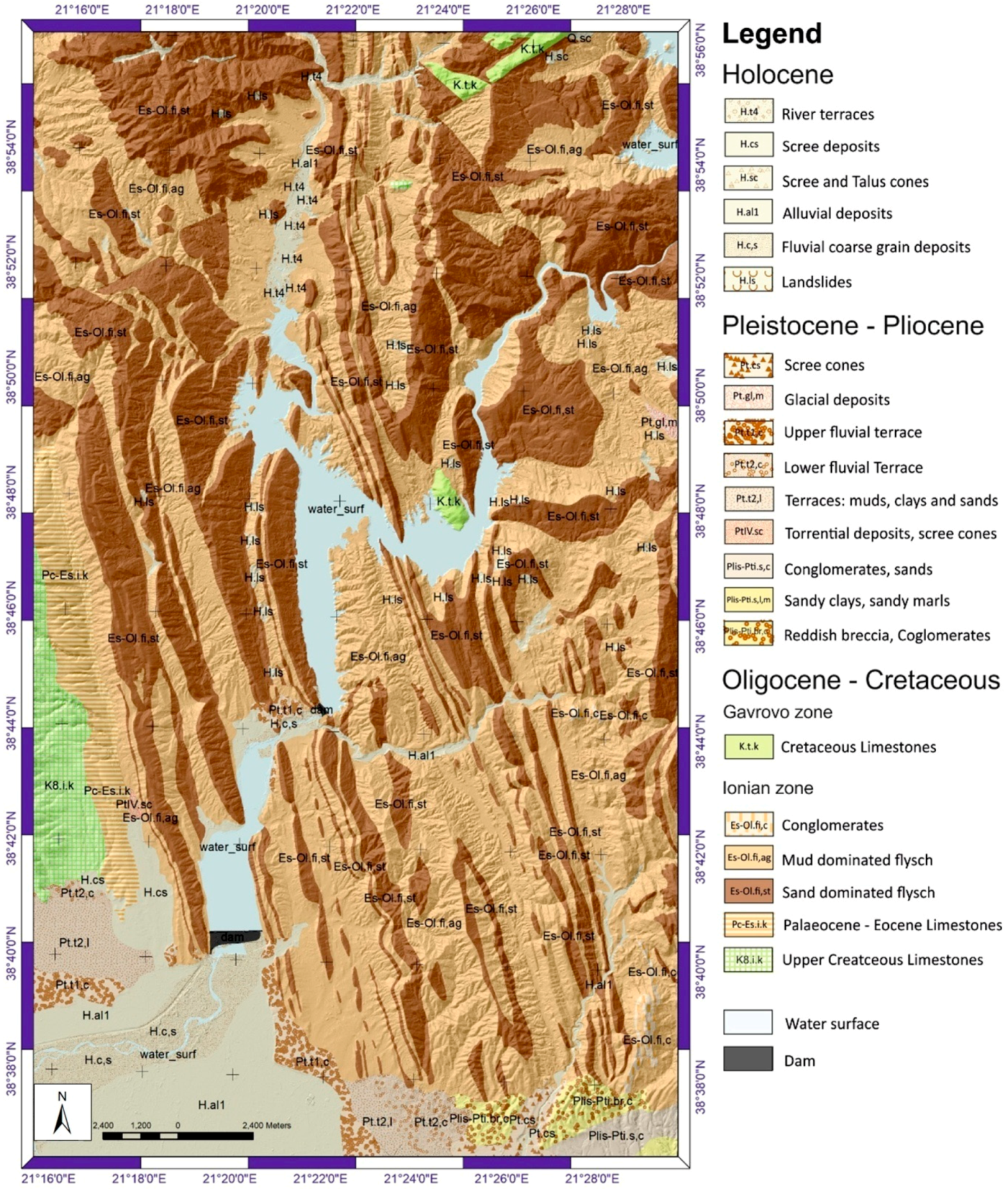
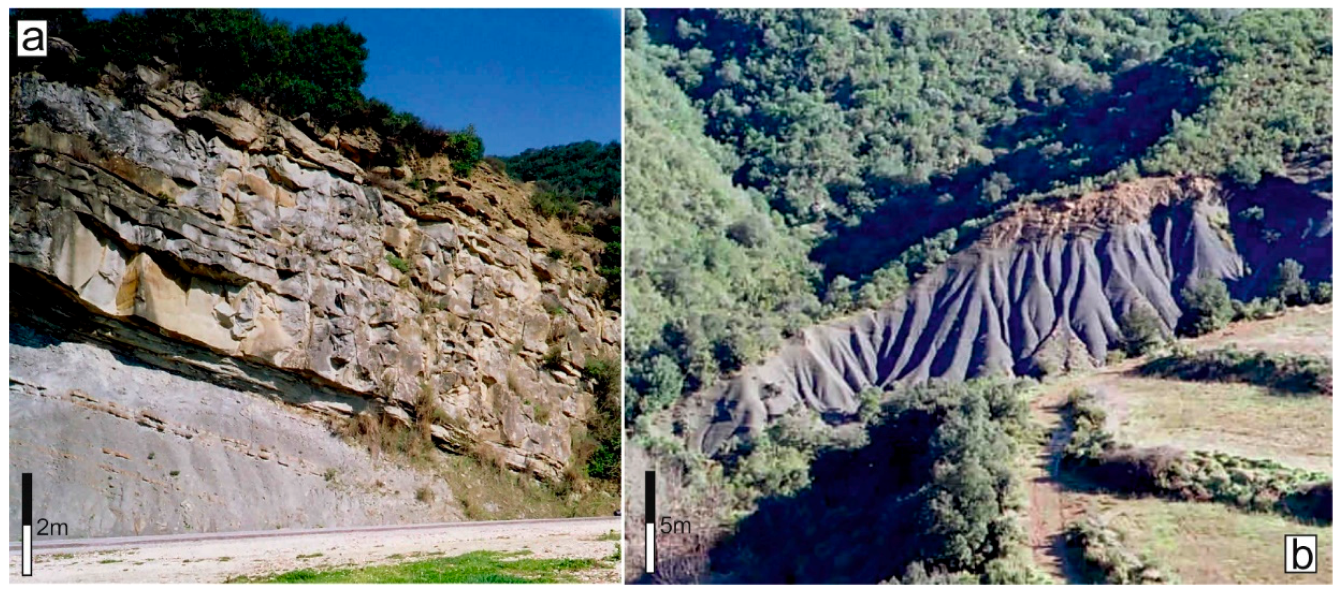
2.1. Study Area
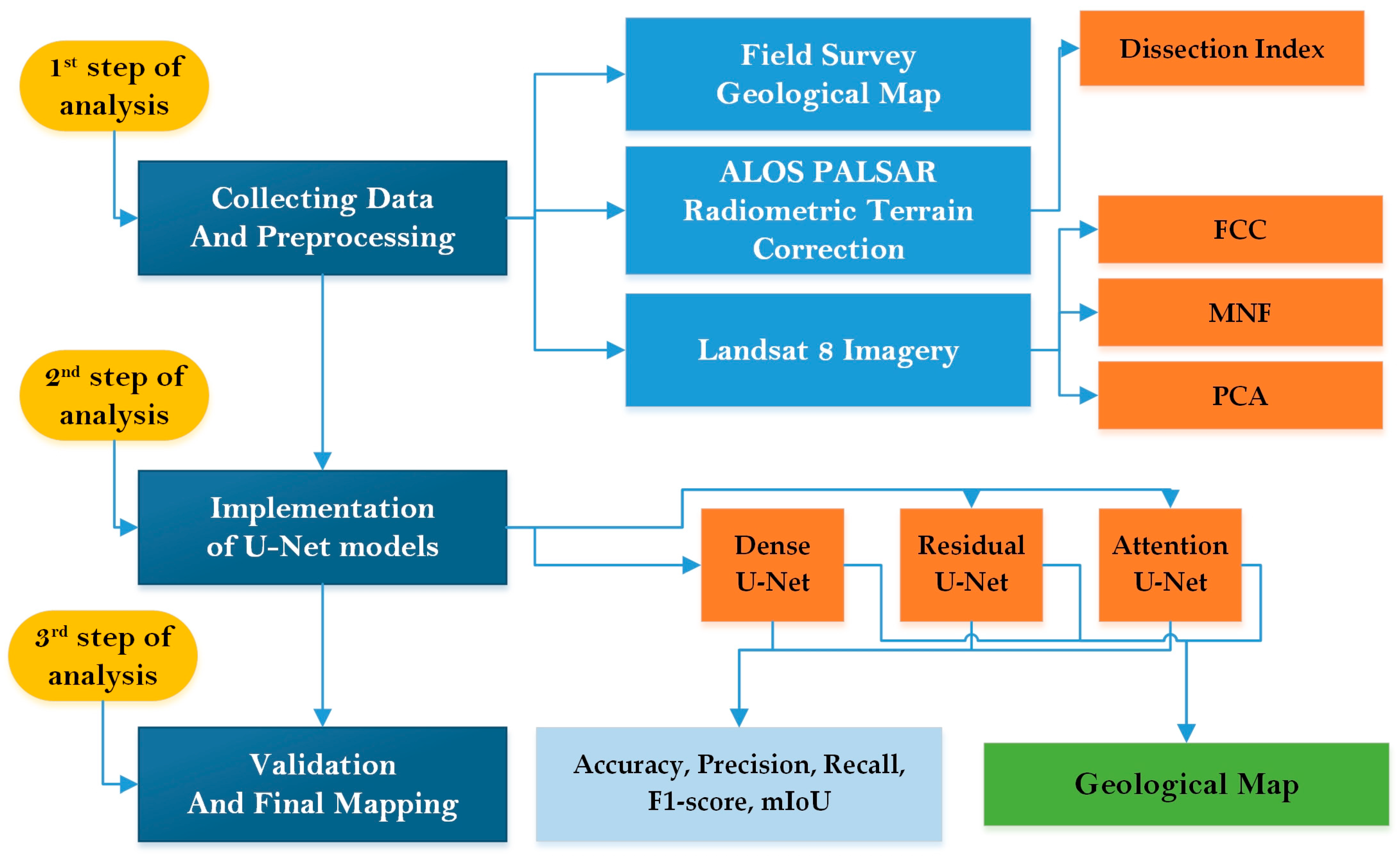
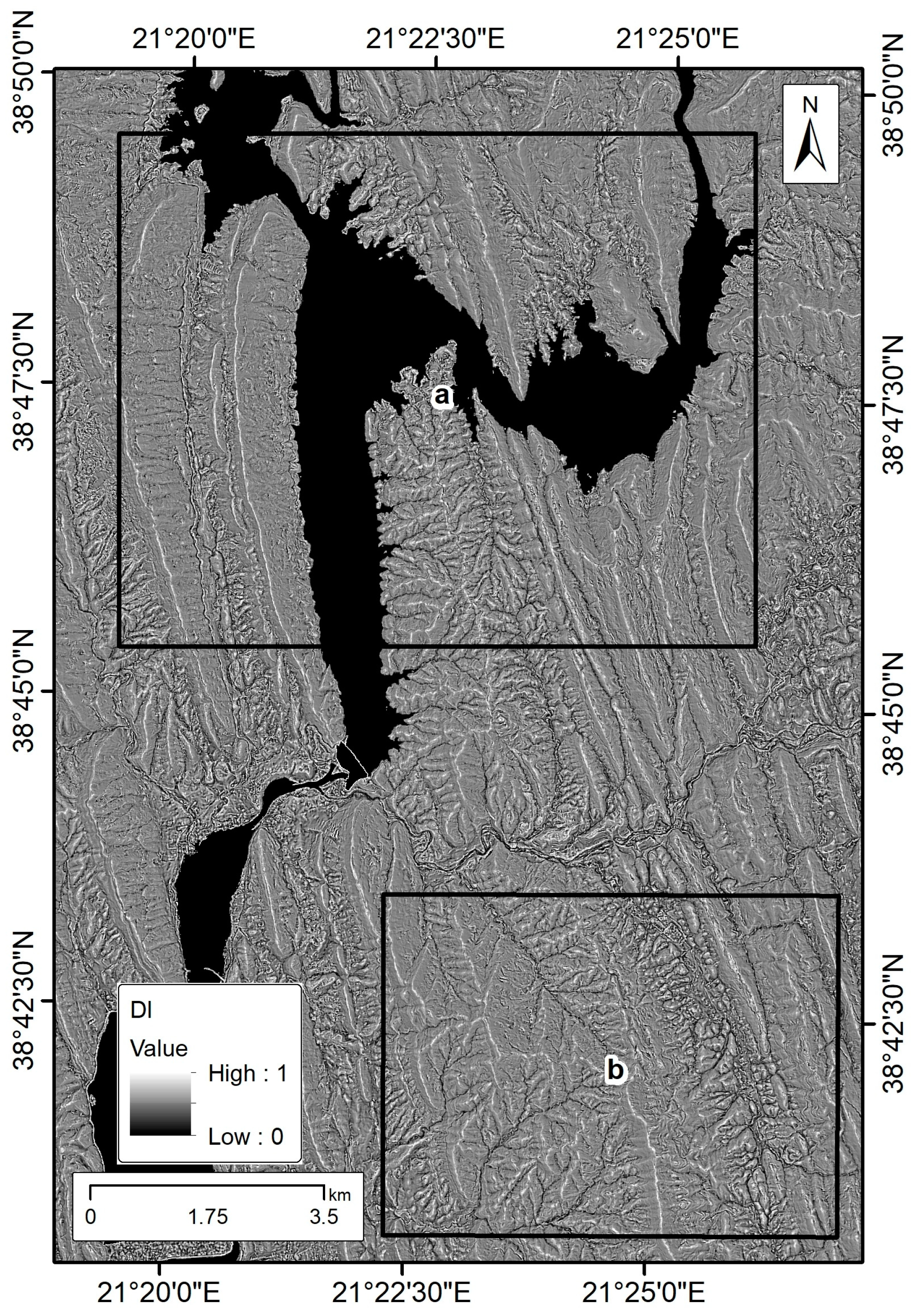
2.2. Methodology
2.2.1. Collect and Preprocessing Data
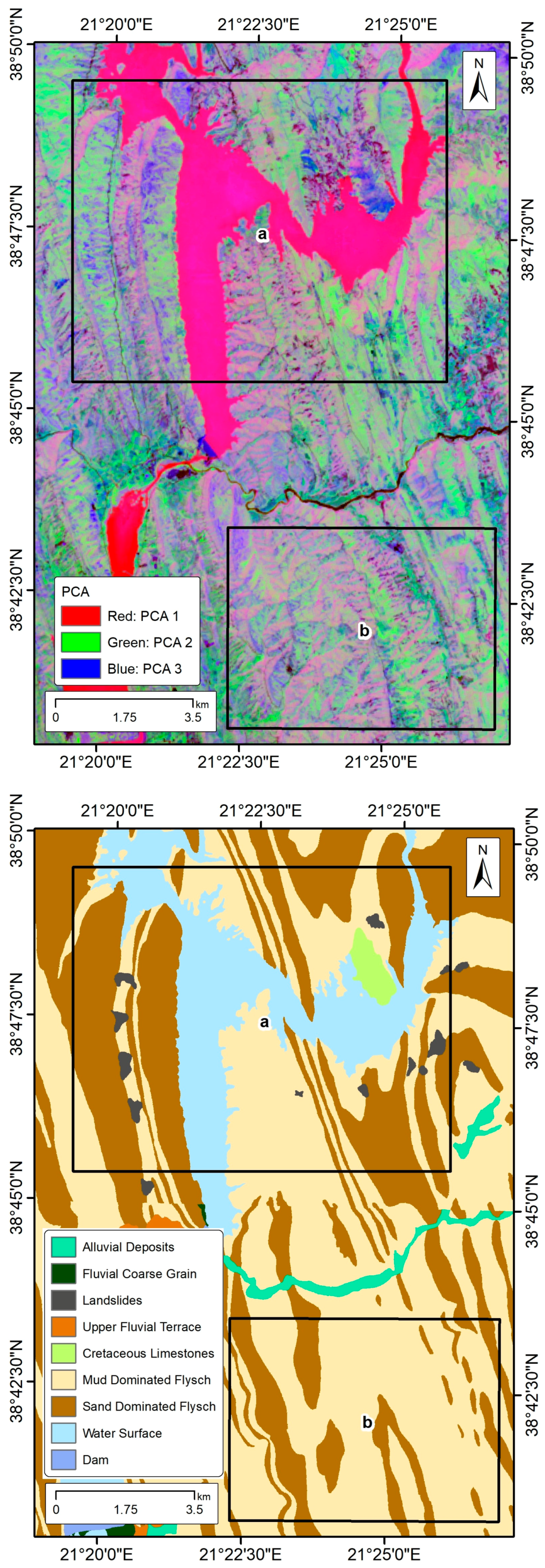
Field Survey—Geological Survey—Ground Truth Data
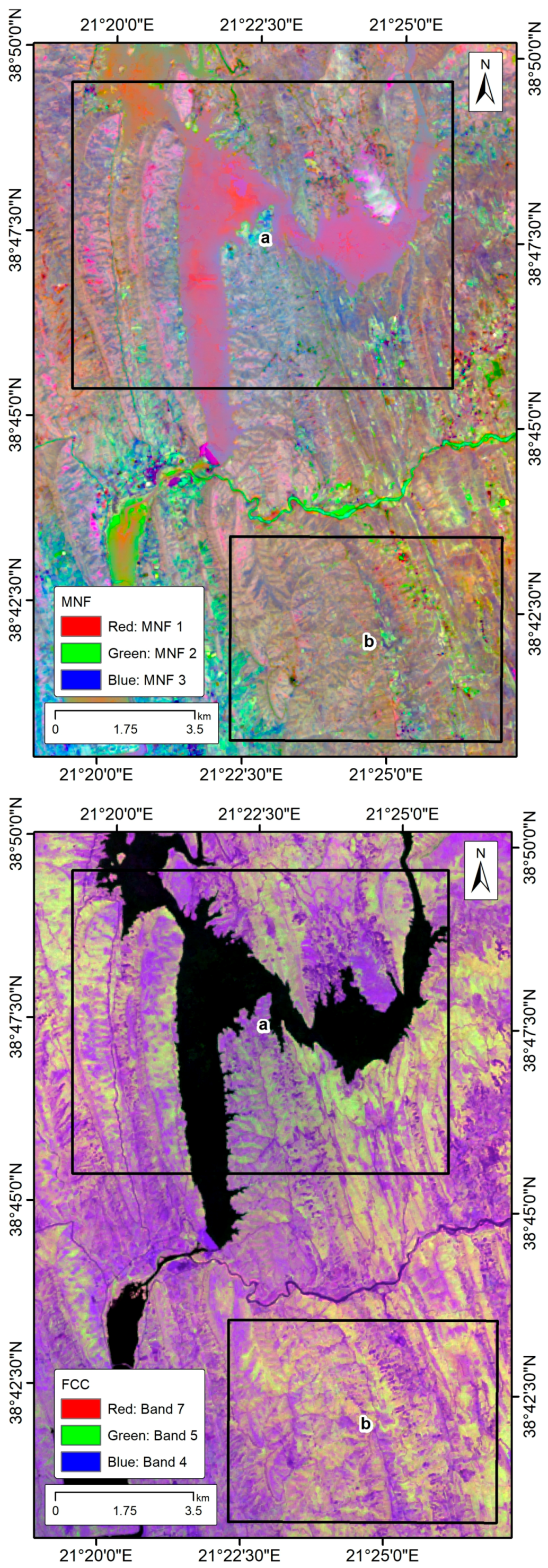
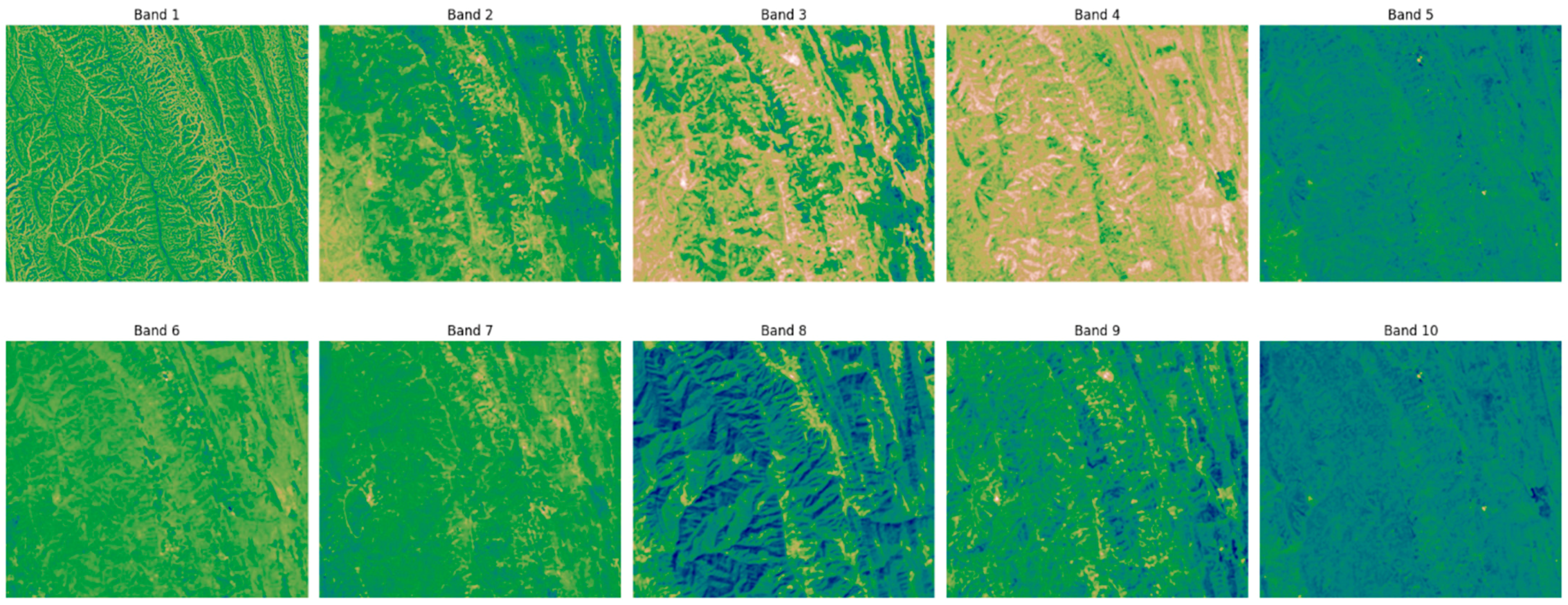
Remote Sensing Data
2.2.2. Training and Validation Database
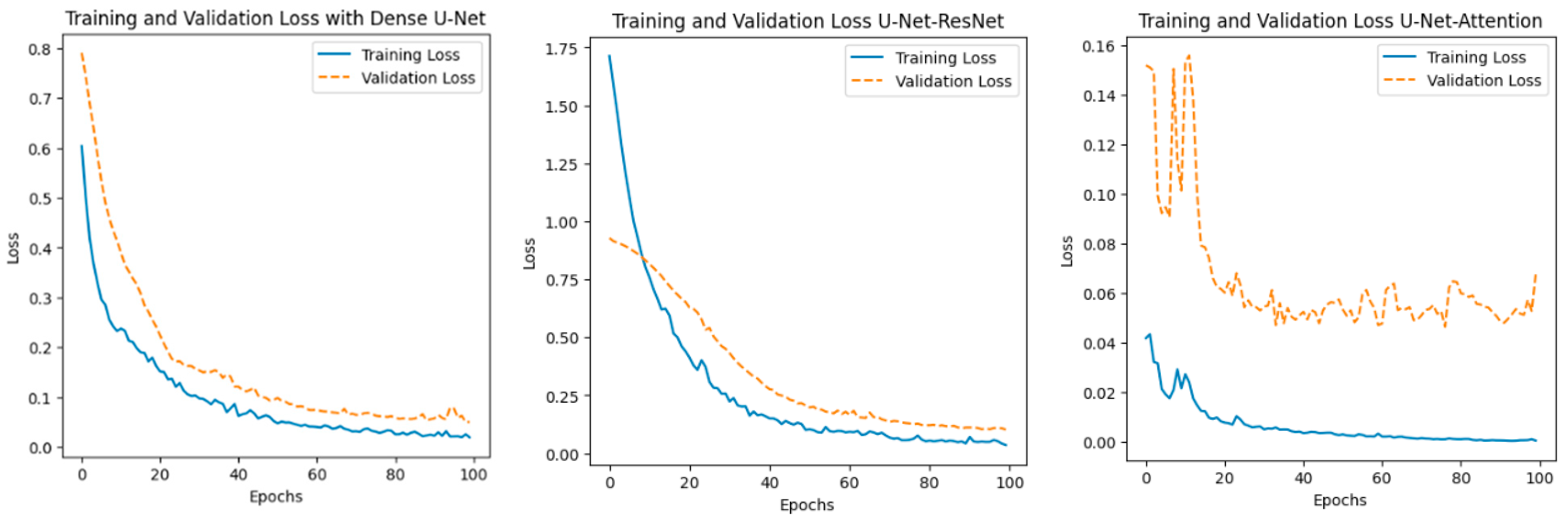
2.2.3. Implementation of U-Net Models
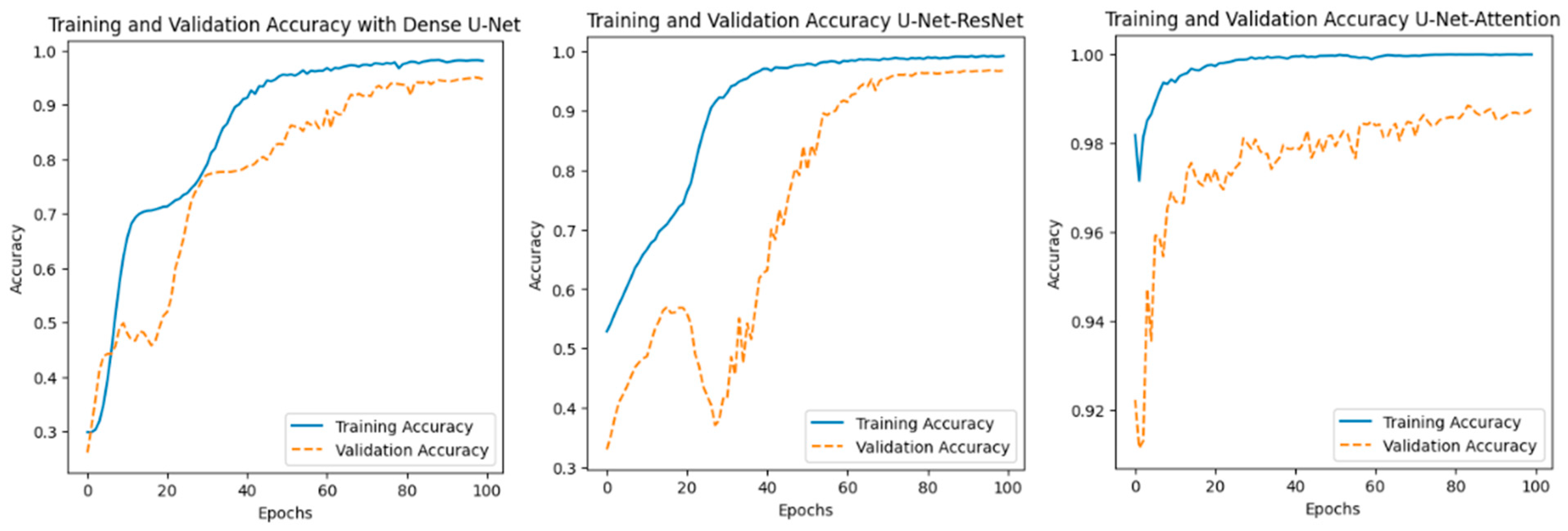
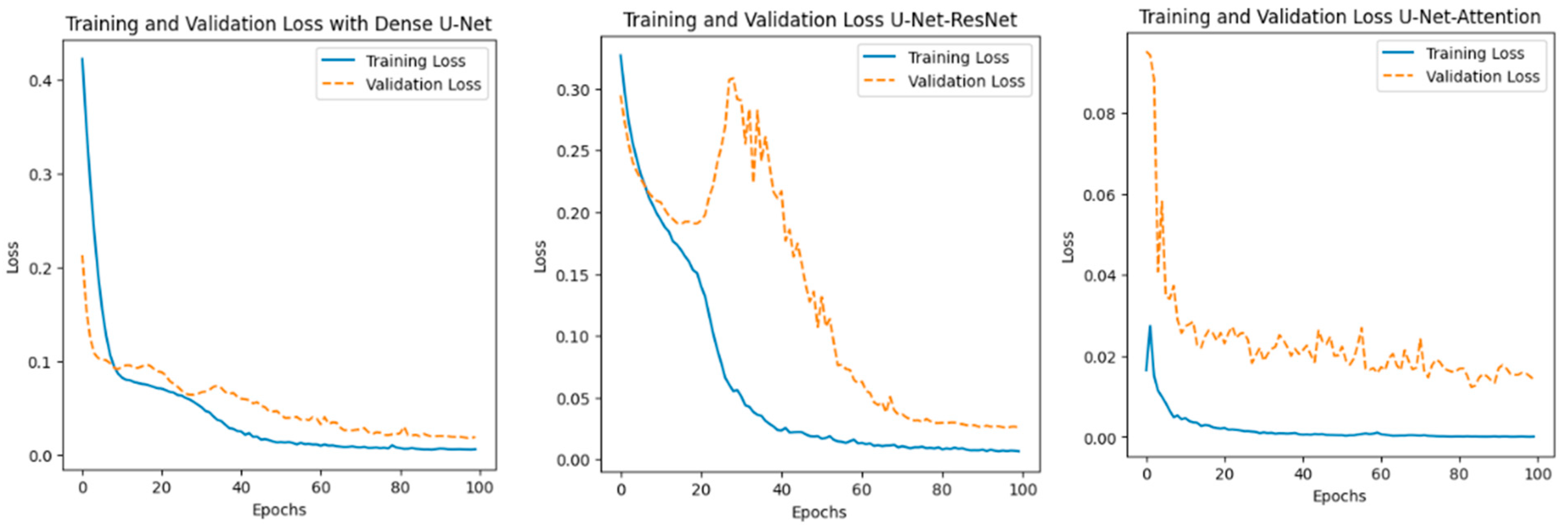
Dense U-Net
Residual U-Net
Attention U-Net
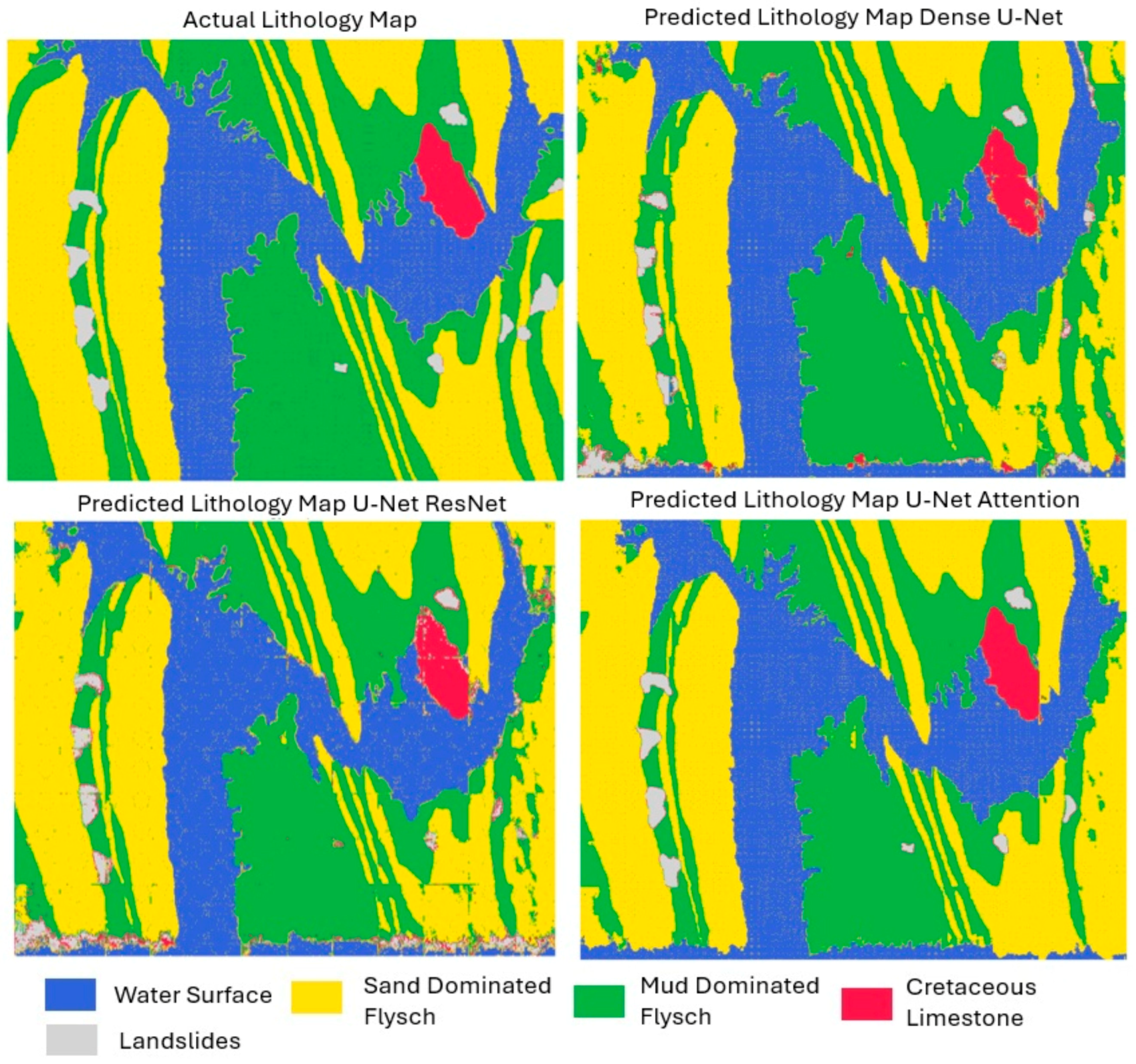
2.2.4. Validation and Final Mapping
3. Results
4. Discussion
5. Conclusions
Author Contributions
Funding
Data Availability Statement
Conflicts of Interest
References
- Peyghambari, S.; Zhang, Y. Hyperspectral Remote Sensing in Lithological Mapping, Mineral Exploration, and Environmental Geology: An Updated Review. J. Appl. Remote Sens. 2021, 15, 031501. [Google Scholar] [CrossRef]
- Mahmood, T.; Hasan, K.; Akhter, S. Lithologic Mapping of a Forested Montane Terrain from Landsat 5 TM Image. Geocarto Int. 2018, 34, 750–768. [Google Scholar] [CrossRef]
- Pal, M.; Rasmussen, T.; Porwal, A. Optimized Lithological Mapping from Multispectral and Hyperspectral Remote Sensing Images Using Fused Multi-classifiers. Remote Sens. 2020, 12, 177. [Google Scholar] [CrossRef]
- Bachri, I.; Hakdaoui, M.; Raji, M.; Teodoro, A.C.; Benbouziane, A. Machine Learning Algorithms for Automatic Lithological Mapping Using Remote Sensing Data: A Case Study from Souk Arbaa Sahel, Sidi Ifni Inlier, Western Anti-Atlas, Morocco. ISPRS Int. J. Geo-Inf. 2019, 8, 248. [Google Scholar] [CrossRef]
- Pour, A.B.; Hashim, M.; Hong, J.K.; Park, Y. Lithological and alteration mineral mapping in poorly exposed lithologies using Landsat-8 and ASTER satellite data: North-eastern Graham Land, Antarctic Peninsula. Ore Geol. Rev. 2019, 108, 112–133. [Google Scholar] [CrossRef]
- Dong, Y.; Yang, Z.; Liu, Q.; Zuo, R.; Wang, Z. Fusion of GaoFen-5 and Sentinel-2B Data for Lithological Mapping Using Vision Transformer Dynamic Graph Convolutional Network. Int. J. Appl. Earth Obs. Geoinf. 2024, 129, 103780. [Google Scholar] [CrossRef]
- Othman, A.A.; Gloaguen, R. Integration of spectral, spatial and morphometric data into lithological mapping: A comparison of different Machine Learning Algorithms in the Kurdistan Region, NE Iraq. J. Asian Earth Sci. 2017, 146, 90–102. [Google Scholar] [CrossRef]
- Cracknell, M.J.; Reading, A.M. Geological mapping using remote sensing data: A comparison of five machine learning algorithms, their response to variations in the spatial distribution of training data and the use of explicit spatial information. Comput. Geosci. 2014, 63, 22–33. [Google Scholar] [CrossRef]
- Sahoo, S.; Jha, M.K. Pattern recognition in lithology classification: Modeling using neural networks, self-organizing maps and genetic algorithms. Hydrogeol. J. 2017, 25, 311–330. [Google Scholar] [CrossRef]
- El-Omairi, M.A.; El Garouani, A. Advancements in Lithological Mapping Utilizing Machine Learning Algorithms and Remote Sensing Data. Heliyon 2023, 9, e20168. [Google Scholar] [CrossRef]
- Manap, H.S.; San, B.T. Data Integration for Lithological Mapping Using Machine Learning Algorithms. Earth Sci. Inform. 2022, 15, 1841–1859. [Google Scholar] [CrossRef]
- Muzirafuti, A. Remotely Sensed and Field Data for Geomorphological Analysis of Water Springs: A Case Study of Ain Maarrouf. Geosciences 2024, 14, 51. [Google Scholar] [CrossRef]
- Appiah-Twum, M.; Xu, W.; Sunkari, E.D. Mapping Lithology with Hybrid Attention Mechanism–Long Short-Term Memory: A Hybrid Neural Network Approach Using Remote Sensing and Geophysical Data. Remote Sens. 2024, 16, 4613. [Google Scholar] [CrossRef]
- Kattenborn, T.; Leitloff, J.; Schiefer, F.; Hinz, S. Review on Convolutional Neural Networks (CNN) in Vegetation Remote Sensing. ISPRS J. Photogramm. Remote Sens. 2021, 173, 24–49. [Google Scholar] [CrossRef]
- Wang, Z.; Zuo, R.; Liu, H. Lithological Mapping Based on Fully Convolutional Network and Multi-Source Geological Data. Remote Sens. 2021, 13, 4860. [Google Scholar] [CrossRef]
- Sarker, I.H. Deep Learning: A Comprehensive Overview on Techniques, Taxonomy, Applications and Research Directions. SN Comput. Sci. 2021, 2, 420. [Google Scholar] [CrossRef]
- Deng, L.; Yu, D. Deep Learning: Methods and Applications. Found. Trends Signal Process. 2014, 7, 197–387. [Google Scholar] [CrossRef]
- Fu, G.; Liu, C.; Zhou, R.; Sun, T.; Zhang, Q. Classification for high resolution remote sensing imagery using a fully convolutional network. Remote Sens. 2017, 9, 498. [Google Scholar] [CrossRef]
- Carranza-García, M.; García-Gutiérrez, J.; Riquelme, J. A Framework for Evaluating Land Use and Land Cover Classification Using Convolutional Neural Networks. Remote Sens. 2019, 11, 274. [Google Scholar] [CrossRef]
- Tsangaratos, P.; Ilia, I.; Chrysafi, A.-A.; Matiatos, I.; Chen, W.; Hong, H. Applying a 1D Convolutional Neural Network in Flood Susceptibility Assessments—The Case of the Island of Euboea, Greece. Remote Sens. 2023, 15, 3471. [Google Scholar] [CrossRef]
- Ronneberger, O.; Fischer, P.; Brox, T. U-net: Convolutional networks for biomedical image segmentation. In Proceedings of the International Conference on Medical Image Computing and Computer-Assisted Intervention, Munich, Germany, 5–9 October 2015; pp. 234–241. [Google Scholar]
- Liu, P.; Wei, Y.; Wang, Q.; Chen, Y.; Xie, J. Research on Post-Earthquake Landslide Extraction Algorithm Based on Improved U-Net Model. Remote Sens. 2020, 12, 894. [Google Scholar] [CrossRef]
- Clark, A.; Phinn, S.; Scarth, P. Optimised U-Net for Land Use–Land Cover Classification Using Aerial Photography. PFG J. Photogramm. Remote Sens. Geoinf. Sci. 2023, 91, 125–147. [Google Scholar] [CrossRef]
- Liu, L.; Song, Z.; Zhou, P.; He, X.; Zhao, L. AI-based rock strength assessment from tunnel face images using hybrid neural networks. Sci. Rep. 2024, 14, 17512. [Google Scholar] [CrossRef] [PubMed]
- Polat, A.; Keskin, İ.; Polat, Ö. Automatic Detection and Mapping of Dolines Using U-Net Model from Orthophoto Images. ISPRS Int. J. Geo-Inf. 2023, 12, 456. [Google Scholar] [CrossRef]
- Chen, W.; Li, X.; Qin, X.; Wang, L. Geological Lithology Semantic Segmentation Based on Deep Learning Method. In Remote Sensing Intelligent Interpretation for Geology; Springer: Singapore, 2024. [Google Scholar] [CrossRef]
- Ghoneim, S.M.; Hamimi, Z.; Abdelrahman, K.; Khalifa, M.A.; Shabban, M.; Abdelmaksoud, A.S. Machine learning and remote sensing-based lithological mapping of the Duwi Shear-Belt area, Central Eastern Desert, Egypt. Sci. Rep. 2024, 14, 17010. [Google Scholar] [CrossRef] [PubMed]
- Le, Y.; Porwal, A.; Holden, E.-J.; Dentith, M.C. Towards Automatic Lithological Classification from Remote Sensing Data Using Support Vector Machines. Comput. Geosci. 2012, 45, 229–239. [Google Scholar] [CrossRef]
- Vakalas, I.; Tripsanas, E.; Tzimeas, C.; Konstantopoulos, P. Sedimentary Characteristics and Basin Evolution of a Compart-mentalized Foreland Basin—Internal Ionian Zone, Western Greece. Energies 2024, 17, 315. [Google Scholar] [CrossRef]
- Underhill, J.R. Neogene and Quaternary Tectonics and Sedimentation in Western Greece. Ph.D. Thesis, University of Wales, Cardiff, UK, 1985. [Google Scholar]
- Aubouin, J. Contribution à l’Étude Géologique de la Grèce Septentrionale: Le Confins de l’Épire et de la Thessalie. Ann. Géologiques Pays Helléniques 1959, 10, 525. [Google Scholar]
- Institute of Geology and Subsurface Research, Greece; Institut Français Pétrole. Étude Géologique de l’Épire (Grèce Nord-Occidentale); Technip: Paris, France, 1966; p. 306. [Google Scholar]
- Avdis, V.; Georgiou Ch Skourtsi-Koroneou, V.; Ioakeim, C.; Leontari, S. Geological Map of Greece in Scale 1:50,000, “Agrinion” Sheet; Institute of Geology and Mineral Exploration: Thens, Greece, 2013. [Google Scholar]
- Karfakis, I.; Kanaki-Mauridou, F.; Tsaila-Monopoli, S. Geological Map of Greece in Scale 1:50,000, “Alevrada” Sheet; Institute of Geology and Mineral Exploration: Athens, Greece, 1989. [Google Scholar]
- Smith, A.G. Othris, Pindos and Vourinos Ophiolites and the Pelagonian Zone. In Proceedings of the VI Colloquium Geology Aegean Region, Athens, Greece; 1977; pp. 1369–1374. [Google Scholar]
- Robertson, A.H.F.; Clift, P.D.; Degnan, P.J.; Jones, G. Palaeogeographic and Palaeotectonic Evolution of the Eastern Mediterranean Neotethys. Palaeogeogr. Palaeoclimatol. Palaeoecol. 1991, 87, 289–343. [Google Scholar] [CrossRef]
- Papanikolaou, D. Timing of Tectonic Emplacement of the Ophiolites and Terrane Paleogeography in the Hellenides. Lithos 2009, 108, 262–280. [Google Scholar] [CrossRef]
- Ricci Lucchi, F. Depositional Cycles in the Two Turbidite Formations of Northern Apennines. J. Sediment. Petrol. 1975, 45, 3–43. [Google Scholar] [CrossRef]
- Ricci Lucchi, F. The Foreland Basin System of the Northern Apennines and Related Clastic Wedges: A Preliminary Outline. G. Geol. 1986, 48, 165–185. [Google Scholar]
- Vakalas, I. The Evolution of Foreland Basins in Western Greece. Ph.D. Thesis, University of Patras, Patras, Greece, 2003; p. 373. [Google Scholar]
- Jacobshagen, V.; Richter, D.; Makris, J. Alpidic Development of the Peloponnesus. In Alps, Apennines, Hellenides; Closs, H., Roeder, D., Schmidt, H., Eds.; E. Schweizerbart’sche Verlagsbuchhandlung: Stuttgart, Germany, 1978; pp. 415–423. [Google Scholar]
- de Graciansky, P.C.; Dardeau, G.; Lemoine, M.; Tricart, P. The Inverted Margin of the French Alps and Foreland Basin Inversion. In Inversion Tectonics; Cooper, M.A., Williams, G.D., Eds.; Geological Society, Special Publication: London, UK, 1989; Volume 44, pp. 87–104. [Google Scholar]
- Doutsos, T.; Koukouvelas, I.K.; Xypolias, P. A New Orogenic Model for the External Hellenides. Geol. Soc. Lond. Spec. Publ. 2006, 260, 507–520. [Google Scholar] [CrossRef]
- Weimer, P.; Pettingill, H.S. Deep-Water Exploration and Production: A Global Overview. In Atlas of Deep-Water Outcrops; AAPG Studies in Geology; American Association of Petroleum Geologists: Tulsa, OK, USA, 2007; Volume 56, pp. 12–16. [Google Scholar]
- Piper, D.J.W.; Panagos, A.G.; Pe, G.G. Conglomeratic Miocene Flysch, Western Greece. J. Sediment. Petrol. 1978, 48, 117–126. [Google Scholar]
- Pavlopoulos, A. Contribution to the Geological Investigation of Makrynoros Flysch Deposits, Akarnania. Ph.D. Thesis, Aristotle University of Thessaloniki, Thessaloniki, Greece, 1983. [Google Scholar]
- Leigh, S.P. The Sedimentary Evolution of the Pindos Foreland Basin, Western Greece. Ph.D. Thesis, University of Wales, Cardiff, UK, 1991. [Google Scholar]
- Leigh, S.P.; Hartley, A.J. Mega-Debris Flow Deposits from the Oligo-Miocene Pindos Foreland Basin, Western Mainland, Greece: Implications for Transport Mechanisms in Ancient Deep Marine Basins. Sedimentology 1992, 39, 1003–1012. [Google Scholar] [CrossRef]
- Avramidis, P.; Zelilidis, A.; Vakalas, I.; Kontopoulos, N. Interactions between Tectonic Activity and Eustatic Sea-Level Changes in the Pindos and Mesohellenic Basins, NW Greece: Basin Evolution and Hydrocarbon Potential. J. Petrol. Geol. 2002, 25, 53–82. [Google Scholar] [CrossRef]
- Konstantopoulos, P.A.; Zelilidis, A. Sedimentation of Submarine Fan Deposits in the Pindos Foreland Basin, from Late Eocene to Early Oligocene, West Peloponnesus Peninsula, SW Greece. Geol. J. 2013, 48, 335–362. [Google Scholar] [CrossRef]
- British Petroleum Co. Ltd. (B.P.). The Geological Results of Petroleum Exploration in Western Greece; Institute for Geology and Subsurface Research: Athens, Greece, 1971; Special Report 10. [Google Scholar]
- Fleury, J.J. Evolution d’une Plateforme et d’un Bassin dans Leur Cadre Alpin: Les Zones de Gavrovo-Tripolitze et du Pinde-Olonos. Soc. Géol. Nord Spec. Publ. 1980, 4, 651. [Google Scholar]
- Wilpshaar, M. Applicability of Dinoflagellate Cyst Stratigraphy to the Analyses of Passive and Active Tectonic Settings. Ph.D. Thesis, University of Utrecht, Utrecht, The Netherlands, 1995. [Google Scholar]
- Bellas, S.M. Calcareous Nannofossils of the Tertiary Flysch (Post-Eocene to Early Miocene) of the Ionian Zone in Epirus NW-Greece: Taxonomy and Biostratigraphical Correlations. In Berliner Geowissenschaftliche Abhandlungen; Selbstverlag Fachbereich Geowissenschaften: Berlin, Germany, 1997; Volume 22, p. 173. [Google Scholar]
- Kaggle. Kaggle: Your Machine Learning and Data Science Community. Available online: https://www.kaggle.com (accessed on 19 January 2025).
- Python Software Foundation. Python Programming Language, Version 3.10. Available online: https://www.python.org (accessed on 19 January 2025).
- De Vries, B.; Huang, C.; Armston, J.; Huang, W.; Jones, J.W.; Lang, M.W. Rapid and robust monitoring of flood events using Sentinel-1 and Landsat data on the Google Earth Engine. Remote Sens. Environ. 2020, 240, 111664. [Google Scholar] [CrossRef]
- Shekar, P.R.; Mathew, A. Morphometric Analysis of Watersheds: A Comprehensive Review of Data Sources, Quality, and Geospatial Techniques. Watershed Ecol. Environ. 2023, 6, 13–25. [Google Scholar] [CrossRef]
- Evans, I.S. General geomorphometry, derivatives of altitude, and descriptive statistics. In Spatial Analysis in Geomorphology; Chorley, R.J., Ed.; Harper & Row: New York, NY, USA, 1972; pp. 17–90. [Google Scholar]
- Singh, S.; Dubey, A. Geoenvironmental Planning of Watersheds in Indian; Chugh Publications: Allahabad, India, 1994; pp. 28–69. [Google Scholar]
- Pike, R.J.; Wilson, S.E. Elevation relief ratio, hypsometric integral and geomorphic area altitude analysis. Bull. Geol. Soc. Am. 1971, 82, 1079–1084. [Google Scholar] [CrossRef]
- ASF-ALOS PALSAR. ALOS PALSAR Overview. Available online: https://asf.alaska.edu/data-sets/sar-data-sets/alos-palsar/ (accessed on 10 December 2024).
- Adiri, Z.; Lhissou, R.; Maacha, L.; Jilali, A.; Talbi, E.H.; Jellouli, A.; Chakouri, M. Comparison of ASTER GDEM3, SRTM3, NASADEM, TanDEM-X90, AW3D30, and ALOS PALSAR Data with TanDEM-X12: A Case Study of Tagragra of Akka Inlier, Moroccan Anti-Atlas. Arab. J. Geosci. 2022, 15, 1654. [Google Scholar] [CrossRef]
- Mwaniki, M.W.; Moeller, M.S.; Schellmann, G. A Comparison of Landsat 8 (OLI) and Landsat 7 (ETM+) in Mapping Geology and Visualising Lineaments: A Case Study of Central Region Kenya. In Proceedings of the 36th International Symposium on Remote Sensing of Environment, Berlin, Germany, 11–15 May 2015. ISRSE36-61. [Google Scholar]
- Qasim, M. Application of Remote Sensing for Geological Mapping Using Landsat Etm+ Satellite Image for part of Western Hazara Ranges Across Siran River, North Pakistan. Pak. J. Hydrocarb. Res. 2024, 26, 1–15. [Google Scholar]
- Sabins, F.F. Remote Sensing Principles and Interpretation; W.H. Freeman Company: New York, NY, USA, 1997; pp. 366–371. [Google Scholar]
- Khalifa, A.; Bashir, B.; Çakir, Z.; Kaya, Ş.; Alsalman, A.; Henaish, A. Paradigm of geological mapping of the adıyaman fault zone of eastern turkey using landsat 8 remotely sensed data coupled with PCA, ICA, and MNFA techniques. Int. J. Geo-Inf. 2021, 10, 368. [Google Scholar] [CrossRef]
- Gasmi, A.; Gomez, C.; Zouari, H.; Masse, A.; Ducrot, D. PCA and SVM as geo-computational methods for geological mapping in the southern of Tunisia, using ASTER remote sensing data set. Arab. J. Geosci. 2016, 9, 753. [Google Scholar] [CrossRef]
- Pour, A.B.; Hashim, M. Spectral Transformation of ASTER Data and the Discrimination of Hydrothermal Alteration Minerals in a Semi-Arid Region, SE Iran. Int. J. Phys. Sci. 2011, 6, 2037–2059. [Google Scholar]
- Serbouti, I.; Raji, M.; Hakdaoui, M.; El Kamel, F.; Pradhan, B.; Gite, S.; Alamri, A.; Maulud, K.N.A.; Dikshit, A. Improved Lithological Map of Large Complex Semi-Arid Regions Using Spectral and Textural Datasets within Google Earth Engine and Fused Machine Learning Multi-Classifiers. Remote Sens. 2022, 14, 5498. [Google Scholar] [CrossRef]
- Nielsen, A.A. Kernel maximum autocorrelation factor and minimum noise fraction transformations. IEEE Trans. Image Process. 2011, 20, 612–624. [Google Scholar] [CrossRef] [PubMed]
- Tatar, A.; Haghighi, M.; Zeinijahromi, A. Experiments on Image Data Augmentation Techniques for Geological Rock Type Classification with Convolutional Neural Networks. J. Rock Mech. Geotech. Eng. 2024, 17, 106–125. [Google Scholar] [CrossRef]
- Ghaznavi, A.; Saberioon, M.; Brom, J.; Itzerott, S. Comparative Performance Analysis of Simple U-Net, Residual Attention U-Net, and VGG16-U-Net for Inventory Inland Water Bodies. Appl. Comput. Geosci. 2024, 21, 100150. [Google Scholar] [CrossRef]
- Massironi, M.; Bertoldi, L.; Calafa, P.; Visonà, D.; Bistacchi, A.; Giardino, C.; Schiavo, A. Interpretation and Processing of ASTER Data for Geological Mapping and Granitoid Detection in the Saghro Massif (Eastern Anti-Atlas, Morocco). Geosphere 2008, 4, 736–759. [Google Scholar] [CrossRef]
- Dang, K.B.; Nguyen, M.H.; Nguyen, D.A.; Phan, T.T.H.; Giang, T.L.; Pham, H.H.; Nguyen, T.N.; Tran, T.T.V.; Bui, D.T. Coastal Wetland Classification with Deep U-Net Convolutional Networks and Sentinel-2 Imagery: A Case Study at the Tien Yen Estuary of Vietnam. Remote Sens. 2020, 12, 3270. [Google Scholar] [CrossRef]
- Chen, P.; Su, X.; Liu, M.; Zhu, W. Lensless Computational Imaging Technology Using Deep Convolutional Network. Sensors 2020, 20, 2661. [Google Scholar] [CrossRef]
- Huang, G.; Liu, Z.; Van Der Maaten, L.; Weinberger, K.Q. Densely Connected Convolutional Networks. In Proceedings of the 2017 IEEE Conference on Computer Vision and Pattern Recognition (CVPR), Honolulu, HI, USA, 21–26 July 2017; pp. 2261–2269. [Google Scholar]
- Zhang, K.; Zuo, W.; Chen, Y.; Meng, D.; Zhang, L. Beyond a Gaussian Denoiser: Residual Learning of Deep CNN for Image Denoising. IEEE Trans. Image Process. 2017, 26, 3142–3155. [Google Scholar] [CrossRef]
- Qi, W.; Wei, M.; Yang, W.; Xu, C.; Ma, C. Automatic Mapping of Landslides by the ResU-Net. Remote Sens. 2020, 12, 2487. [Google Scholar] [CrossRef]
- Oktay, O.; Schlemper, J.; Le Folgoc, L.; Lee, M.; Heinrich, M.; Misawa, K.; Mori, K.; McDonagh, S.; Hammerla, N.Y.; Kainz, B.; et al. Attention U-Net: Learning Where to Look for the Pancreas. arXiv 2018, arXiv:1804.03999. [Google Scholar] [CrossRef]
- Abdullah, M.A.M.; Mohammed, A.A.; Awad, S.R. RockDNet: Deep Learning Approach for Lithology Classification. Appl. Sci. 2024, 14, 5511. [Google Scholar] [CrossRef]
- Bahrami, H.; Esmaeili, P.; Homayouni, S.; Pour, A.B.; Chokmani, K.; Bahroudi, A. Machine Learning-Based Lithological Mapping from ASTER Remote-Sensing Imagery. Minerals 2024, 14, 202. [Google Scholar] [CrossRef]
- Long, J.; Shelhamer, E.; Darrell, T. Fully Convolutional Networks for Semantic Segmentation. In Proceedings of the IEEE Conference on Computer Vision and Pattern Recognition, Boston, MA, USA, 7–12 June 2015; pp. 3431–3440. [Google Scholar] [CrossRef]
- Rahman, M.A.; Wang, Y. Optimizing intersection-over-union in deep neural networks for image segmentation. In Proceedings of the International Symposium on Visual Computing, Las Vegas, NV, USA, 12–14 December 2006; Springer: Cham, Switzerland; Berlin/Heidelberg, Germany, 2016; pp. 234–244. [Google Scholar]
- Han, W.; Zhang, X.; Wang, Y.; Wang, L.; Huang, X.; Li, J.; Wang, S.; Chen, W.; Li, X.; Feng, R.; et al. A Survey of Machine Learning and Deep Learning in Remote Sensing of Geological Environment: Challenges, Advances, and Opportunities. ISPRS J. Photogramm. Remote Sens. 2023, 202, 87–113. [Google Scholar] [CrossRef]
- Sun, W.; Zhou, J.; Meng, X.; Yang, G.; Ren, K.; Peng, J. Coupled Temporal Variation Information Estimation and Resolution Enhancement for Remote Sensing Spatial–Temporal–Spectral Fusion. IEEE Trans. Geosci. Remote Sens. 2023, 61, 5532118. [Google Scholar] [CrossRef]
- Blaschke, T.; Kelly, M.; Merschdorf, H. Object-based image analysis: Evolution, history, state of the art, and future vision. In Remotely Sensed Data Characterization, Classifcation, and Accuracies; Thenkabail, P.S., Ed.; UC: Berkeley, CA, USA, 2015. [Google Scholar]
- Pandey, P.C.; Koutsias, N.; Petropoulos, G.P.; Srivastava, P.K.; Dor, E.B. Land use/land cover in view of earth observation: Data sources, input dimensions, and classifers–a review of the state of the art. Geocarto Int. 2021, 36, 957–988. [Google Scholar] [CrossRef]
- Ma, X.; Wang, H.; Wang, J. Semisupervised classification for hyperspectral image based on multi-decision labeling and deep feature learning. ISPRS J. Photogramm. Remote Sens. 2016, 120, 99–107. [Google Scholar] [CrossRef]
- Ma, L.; Liu, Y.; Zhang, X.; Ye, Y.; Yin, G.; Johnson, B.A. Deep learning in remote sensing applications: A meta-analysis and review. ISPRS J. Photogramm. Remote Sens. 2019, 152, 166–177. [Google Scholar] [CrossRef]
- Giang, T.L.; Dang, K.B.; Le, Q.T.; Nguyen, V.G.; Tong, S.S.; Pham, V.-M. U-Net Convolutional Networks for Mining Land Cover Classification Based on High-Resolution UAV Imagery. IEEE Access 2020, 8, 186257–186273. [Google Scholar] [CrossRef]
- Diakogiannis, F.I.; Waldner, F.; Caccetta, P.; Wu, C. ResUNet–A: A Deep Learning Framework for Semantic Segmentation of Remotely Sensed Data. ISPRS J. Photogramm. Remote Sens. 2020, 162, 94–114. [Google Scholar] [CrossRef]


| Models | Overall Accuracy % | Overall IoU % |
|---|---|---|
| Dense U-Net | 0.8993 | 0.7459 |
| Residual U-Net | 0.9247 | 0.8517 |
| Attention U-Net | 0.9597 | 0.9320 |
| Models |
Landslide Body |
Cretaceous Limestone |
Mud-Dominated Flysch |
Sand-Dominated Flysch |
Water Body |
|---|---|---|---|---|---|
| Dense U-Net |
Precision: 0.7282 Recall: 0.3765 F1-score: 0.4964 |
Precision: 0.9717 Recall: 0.8871 F1-score: 0.9274 |
Precision: 0.9043 Recall: 0.8384 F1-score: 0.8701 |
Precision: 0.8737 Recall: 0.9628 F1-score: 0.9161 |
Precision: 0.9589 Recall: 0.9573 F1-score: 0.9581 |
| Residual U-Net |
Precision: 0.8511 Recall: 0.8607 F1-score: 0.8559 |
Precision: 0.9610 Recall: 0.9345 F1-score: 0.9476 |
Precision: 0.9298 Recall: 0.8610 F1-score: 0.8941 |
Precision: 0.9072 Recall: 0.9553 F1-score: 0.9307 |
Precision: 0.9547 Recall: 0.9744 F1-score: 0.9645 |
| Attention U-Net |
Precision: 0.9979 Recall: 0.9365 F1-score: 0.9662 |
Precision: 0.9741 Recall: 0.9963 F1-score: 0.9851 |
Precision: 0.9784 Recall: 0.8918 F1-score: 0.9331 |
Precision: 0.9208 Recall: 0.9870 F1-score: 0.9528 |
Precision: 0.9798 Recall: 0.9904 F1-score: 0.9851 |
| Models | Overall Accuracy % | Overall IoU % |
|---|---|---|
| Dense U-Net | 0.9476 | 0.8729 |
| Residual U-Net | 0.9683 | 0.9066 |
| Attention U-Net | 0.9877 | 0.9320 |
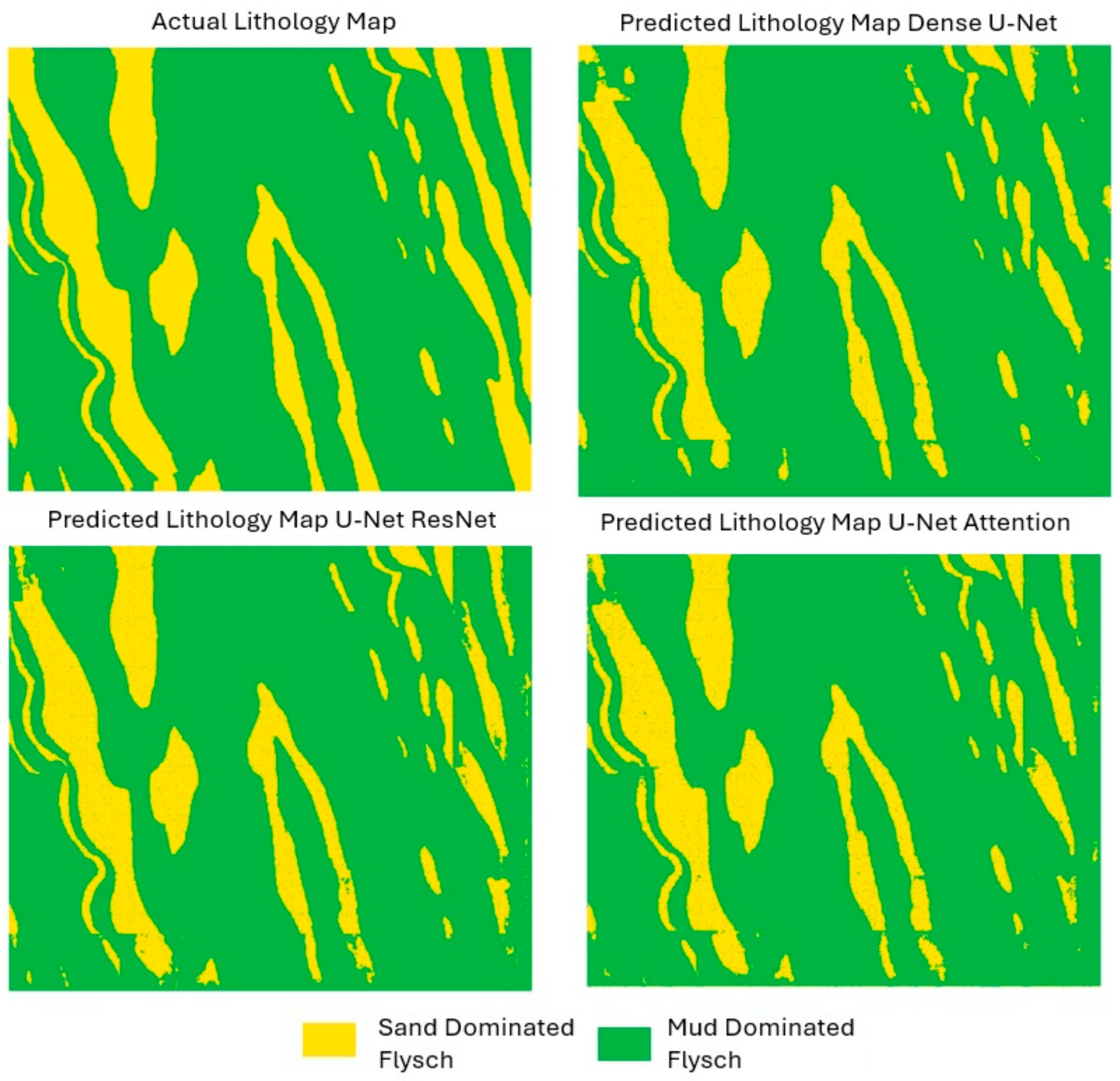
| Models | Mud-Dominated Flysch | Sand-Dominated Flysch |
|---|---|---|
| Dense U-Net | Precision: 0.9582 Recall: 0.9834 F1-score: 0.9706 | Precision: 0.9359 Recall: 0.8489 F1-score: 0.8908 |
| Residual U-Net | Precision: 0.9732 Recall: 0.9835 F1-score: 0.9783 | Precision: 0.9401 Recall: 0.9051 F1-score: 0.9223 |
| Attention U-Net | Precision: 0.9876 Recall: 0.9967 F1-score: 0.9921 | Precision: 0.9882 Recall: 0.9561 F1-score: 0.9719 |
Disclaimer/Publisher’s Note: The statements, opinions and data contained in all publications are solely those of the individual author(s) and contributor(s) and not of MDPI and/or the editor(s). MDPI and/or the editor(s) disclaim responsibility for any injury to people or property resulting from any ideas, methods, instructions or products referred to in the content. |
© 2025 by the authors. Licensee MDPI, Basel, Switzerland. This article is an open access article distributed under the terms and conditions of the Creative Commons Attribution (CC BY) license (https://creativecommons.org/licenses/by/4.0/).
Share and Cite
Tsangaratos, P.; Vakalas, I.; Zanarini, I. Distinguishing Lithofacies of Flysch Formations Using Deep Learning Models: Integrating Remote Sensing Data with Morphological Indexes. Remote Sens. 2025, 17, 422. https://doi.org/10.3390/rs17030422
Tsangaratos P, Vakalas I, Zanarini I. Distinguishing Lithofacies of Flysch Formations Using Deep Learning Models: Integrating Remote Sensing Data with Morphological Indexes. Remote Sensing. 2025; 17(3):422. https://doi.org/10.3390/rs17030422
Chicago/Turabian StyleTsangaratos, Paraskevas, Ioannis Vakalas, and Irene Zanarini. 2025. "Distinguishing Lithofacies of Flysch Formations Using Deep Learning Models: Integrating Remote Sensing Data with Morphological Indexes" Remote Sensing 17, no. 3: 422. https://doi.org/10.3390/rs17030422
APA StyleTsangaratos, P., Vakalas, I., & Zanarini, I. (2025). Distinguishing Lithofacies of Flysch Formations Using Deep Learning Models: Integrating Remote Sensing Data with Morphological Indexes. Remote Sensing, 17(3), 422. https://doi.org/10.3390/rs17030422