A Multilevel Surrogate Model-Based Precipitation Parameter Tuning Method for CAM5 Using Remote Sensing Data for Validation

Abstract

The uncertainty of physical parameters is a major factor contributing to poor precipitation simulation performance in Earth system models (ESMs), particularly in tropical and Pacific regions. To address the high computational cost of repetitive ESM runs, this study proposes a multilevel surrogate model-based parameter optimization framework and applies it to improve the precipitation performance of CAM5. A top-level surrogate model using gradient boosting regression trees (GBRTs) was constructed, leveraging the candidate point (CAND) approach applied to balance exploration and exploitation. A bottom-level surrogate model was then built based on a small, selected dataset; we designed a trust region approach to adjust the sampling region during the bottom-level tuning process. Experimental results demonstrate that the proposed method achieves fast convergence and significantly enhances precipitation simulation accuracy, with an average improvement of 19% in selected regions. In integrating optimization results through a nonuniform parameterization scheme and parameter smoothing, substantial improvements were observed in the South Pacific, Niño, South America, and East Asia. Comparisons with remote sensing data confirm that the optimized precipitation simulations do not introduce significant biases to other variables, validating the effectiveness and robustness of the proposed method.

1. Introduction

Earth system models (ESMs) are an indispensable tool for predicting future climate change trends. In ESMs, because of the grid resolution constraint, physical parameterization schemes are used to describe subgrid physical processes [1]. These subgrid-scale parameterizations encompass multi-faceted interactions with hydro-atmospheric sciences. Each of them contains many uncertain parameters that represent global processes. These parameters control the physical processes at the subgrid scale [2], and slight variations could lead to huge errors in the simulations [3]. Therefore, it is important to calibrate the parameters to better capture real-world physical behaviors [4]. Generally, parameter tuning depends on the experience of climate model experts [5]. However, the physical processes in the Earth system model are becoming increasingly complex as atmospheric science continues to advance. Traditional expertise-based tuning methods may become relatively less applicable in certain contexts.

Automatic optimization algorithms are effective tools with which to replace manual methods. There have been many studies that used various optimization techniques to achieve parameter tuning. Many studies focus on solving the problem; for example, Yang et al. [6] proposed a simulated stochastic approximation annealing (SSAA) [7]-based parameter tuning method. The parameters of the Zhang–McFarlane scheme in CAM5.3 were tuned with SSAA, and there were some positive impacts, including a double intertropical convergence zone and East Asian monsoon precipitation prediction after using the optimal parameters. The authors of [8,9,10] discussed machine learning for ESM calibration and used a machine learning method in both a single-column model and global model. To improve the optimization efficiency, Zhang et al. [11] enhanced the downhill simplex optimization technique, leading to the discovery of a better local minimum solution by selecting more appropriate initial parameter values.

The simulation results of the grid-point atmospheric model of IAP LASG version 2 (GAMIL2), in limited optimal iterations, proved that the downhill simplex method was better than the global optimization algorithms. Williamson et al. [12,13,14] proposed the history-matching method to quantify parametric uncertainty and remove structural biases for the third Hadley Centre Climate Model (HadCM3) and Nucleus for European Modelling of the Ocean (NEMO) ORCA2 global ocean model. Zhang et al. [15] proposed an automated tuning approach that integrates automatic tuning with short-term hindcasts to alleviate the heavy computational workload. The tuning led to a substantial reduction in the significant underestimation of CAM5 longwave cloud forcing and the overestimation of precipitation. Gilewski [16] evaluated the application of Global Environmental Multiscale (GEM) numerical precipitation forecasts in event-based rainfall–runoff hydrological modeling.

These studies indicated that such algorithms can calibrate parameters automatically and effectively improve the simulation accuracy of the ESMs. However, these algorithms typically require a certain number of iterations to meet convergence conditions and find the optimal solution. This means that the quality of the solution depends to some extent on the number of iterations. Typically, ESMs are more complex and resource-consuming than other problems. Therefore, the computational cost generated by such iteration processes is usually unacceptable. Although these methods shorten the optimization time to varying degrees, compared to traditional parameter tuning methods, they still need to run an ESM many times.

Surrogate models are regarded as effective tools with which to solve computationally expensive optimization problems [17]. The objective function in these problems is difficult to express mathematically, or its mathematical form is too complex and time-consuming to compute. The key to solving these problems is to reduce the number of expensive model runs to an acceptable level. A surrogate model establishes connections between adjustable parameters and the responses of a complex expensive model by statistical or data-driven models to approximate a complex expensive model. This is one of the most commonly used approaches for optimizing large complex models. Recently, some studies have indicated that there are various methods with which to construct surrogate models, such as polynomial regression [18], support vector machines [19,20], radial basis function (RBF) networks [21], artificial neural networks (ANNs) [22], and Gaussian processes (GPs) [23,24]. Because the surrogate model can effectively reduce the number of iterations of the objective problem in the optimization process, it is widely used in the parameter optimization of various complex engineering problems.

In recent years, with the development of surrogate model-based optimizations, these methods have been widely used to solve the parameter tuning problems of complex geoscientific models. Neelin et al. [25] constructed a polynomial model that can approximate an atmospheric general circulation model (AGCM) to guide parameter choices. Müller et al. [26] used the RBF surrogate model to optimize the methane emission predictions of a community land model (CLM). Xu et al. [27] proposed a surrogate model-based optimization method to improve the prediction accuracy of the soil organic carbon (SOC) results applying the calibrated parameter values, and result showed that the error could be reduced by up to 12%. Wang et al. [28] established a connection between the optimization of mathematical benchmarks and complex geoscientific models and proposed the adaptive surrogate model-based optimization (ASMO) method. In order to demonstrate the performance of the ASMO method for the parameter tuning of complex geoscientific models, the parameters of a Sacramento Soil Moisture Accounting (SAC-SMA) hydrologic model were tuned based on the ASMO method. On this basis, ASMO has been used to calibrate the parameters of various complex geoscientific models. For example, Gong et al. [29] focused on the Heihe river basin and attempted to tune the parameters that belong to the common land model (CoLM) using a MO-ASMO method. Di et al. [30] implemented the ASMO method to tune WRF model parameters to increase summer precipitation simulations over the Greater Beijing area. Chinta and Balaji [31] presented an MO-ASMO method to enhance the prediction accuracy of the Indian summer monsoon (ISM) in the WRF model. Zhang et al. [32] proposed a land surface evapotranspiration (ET) optimization method based on the multivariate adaptive regression spline (MARS) surrogate model and the ASMO method. The mentioned studies have sufficiently shown that surrogate model-based optimization methods are capable of resolving ESM parameter tuning problems. However, most of these studies focused on weather models or land models, such as the WRF, CoLM and CLM, which cannot prove that surrogate model-based optimization methods are effective for CAM5 parameter tuning. CAM5 is strongly nonlinear and contains more complex physical processes. The application of surrogate models for CAM5 requires further exploration.

CAM5 is a well-calibrated model [15]. Many simulation experiments have indicated that CAM5 captures the global scale of precipitation characteristics reasonably well [33,34]. However, simulation results are still not accurate in some areas. Improving the simulation results over the areas with errors has become one of the biggest CAM5 simulation challenges, and many studies have attempted to improve the CAM5 simulation results over these error areas. Li et al. [35] analyzed the precipitation climatological features over East Asia. Pathak et al. [36] attempted to improve CAM5 precipitation simulation over South Asia. Wang et al. [37] improved the tropical precipitation variability simulation results in CAM5. These studies demonstrated that compared with the default experiment, the simulation results over some regions can be improved to a certain degree. Cui et al. [38], Wang and Zhang [39] conducted studies to improve parameterization schemes by refining physical processes. However, these studies have generally focused on enhancing parameterization schemes from a global perspective, without considering variations across different regions. For these reasons, in this paper, we propose a region-based optimization approach and introduce a nonuniform parameterization scheme, where optimal parameters for multiple regions are integrated into the same case.

The main research contributions of this work are as follows:

1. We first propose a surrogate model-based parameter tuning method for CAM5 precipitation, validating its effectiveness for this complex model.

2. A multilevel surrogate model method is introduced, integrating the candidate point approach and trust region, leading to faster convergence and fewer errors during tuning.

3. A nonuniform parameterization scheme is designed with region-based optimization, improving precipitation simulation by an average of 19% across selected regions.

The structure of this paper is as follows. In Section 2, we provides the details of the experimental design and the description of the model and introduce the surrogate model-based parameter optimization method. In Section 3, we prove the robustness and effectiveness of the surrogate model construction and provide evaluations and analyses of the optimization results. Section 4 comprises the conclusion and discussion.

2. Experimental Setup and Methodology

2.1. Model Description

In this study, we selected the community atmospheric model (CAM Version 5.3), which serves as the atmospheric component of the community Earth system model (CESM, Version 1.3). The compset used in this study was F_2000_CAM5, where “F” means that the active components are atmosphere and land, and “2000” represents the present day period. “CAM5” indicates that the version of the atmospheric model is 5. F_2000_CAM5 is composed of the following components: an active community atmospheric model CAM5.3 and community land model (CLM), a data ocean model (DOCN), and a thermodynamics-only sea ice model (CICE). The model adopts the spectral element dynamical core (SE-dycore) formulation, which is described by Dennis et al. [40]. The resolution was ne30_g16. This means that the model implements a spectral element 1-degree atmosphere and land grids, a gx1v6 Greenland pole 1-degree ocean and sea-ice grids, a 1/2 degree river routing grid, null-wave and internal cism grids, and an ocean/land mask that is determined using the gx1v6 ocean mask.

In this study, a series of AGCM simulations were carried out for 6 years (with 1 year as the model spin-up) for all the simulations. The last 5 years of simulation were used to evaluate the synthesized performance metric of precipitation. The timestep was 1800 s, with the output frequency set to monthly, generating one “.nc” file per simulated month. The resolution was ne30_g16 with 30 vertical layers. We used the climatological SST dataset for the DOCN input data in the CAM5 simulation. The key information of the experimental setup is shown in

Table 1. Introduction to the experimental setup.

Name	Region
Model	Community atmospheric model (CAM Version 5.3)
Compset	F_2000_CAM5
Grid types	Spectral element dynamical core (SE-dycore)
Resolution	ne30_g16
Simulation duration	6 years (with 1 year as the model spin-up)
Timestep	1800 s

.

2.2. Experimental Design

2.2.1. Region Selection and Observation Data

In this study, we selected six regions to improve their precipitation simulation. These regions were selected because they are distributed in the 45° N–45° S region. The majority of global precipitation is concentrated in the mid–low-latitude regions. Tuning parameters over these regions can effectively improve the simulation of CAM5 precipitation. WarmPool, South Pacific, Nino, South America, South Asia, and East Asia were included. Their range is shown in

Table 2. Regions selected in this study.

Name	Region
WarmPool	$-{15}^{\circ }$–${15}^{\circ }$N, 120°–150°E
South Pacific	$-{30}^{\circ }$–$0^{\circ }$N, ${190}^{\circ }$–${250}^{\circ }$E
Nino	$6^{\circ }$–${12}^{\circ }$N, ${210}^{\circ }$–${270}^{\circ }$E
South America	$-{20}^{\circ }$–$0^{\circ }$N, ${280}^{\circ }$–${300}^{\circ }$E
South Asia	$0^{\circ }$–${10}^{\circ }$N, ${75}^{\circ }$–${115}^{\circ }$E
East Asia	${15}^{\circ }$–${40}^{\circ }$N, ${105}^{\circ }$–${140}^{\circ }$E

and Figure 1.

As datasets for evaluating the model precipitation simulation performance, the most commonly used are GPCP [41] and ERA5 [42]. In this study, we selected ERA5. Both ERA5 and GPCP can be used for precipitation analysis. They both provide global precipitation data. However, ERA5 provides higher-resolution data. The data of GPCP are provided on a 2.5-degree grid, and ERA5 precipitation data are provided on a 0.25-degree grid. We believe that choosing data with higher resolution can significantly contrast the tuning results, thereby demonstrating the effectiveness of the proposed method. So, we selected ERA5 instead of GPCP for CAM5 precipitation parameter tuning. The “ESMF_regrid” function and “bilinear” method in the NCAR Command Language (NCL) were used to regrid data.

2.2.2. Parameters and Ranges

The parameter ranges and default values are shown in

Table 3. CAM5 parameter descriptions, default values, and ranges. The CAPE represents the convective available potential energy.

Parameter	Description	Range	Default
cldfrc_rhminl	Relative humidity threshold for stratiform low clouds	0.80∼0.99	0.8975
zmconv_dmpdz	Parcel fractional mass entrainment rate (m−1)	$-2.0\times {10}^{-3}$∼$-0.2\times {10}^{-3}$	$-1.0\times {10}^{-3}$
zmconv_c0_ocn	Deep convection precipitation efficiency over the ocean	$1.0\times {10}^{-3}$∼0.1	$0.045$
zmconv_tau	Time scale for consumption rate of deep CAPE (s)	1800∼28,800	3600
micro_mg_dcs	Auto conversion size threshold for ice to snow (m)	$100\times {10}^{-6}$∼$500\times {10}^{-6}$	$400\times {10}^{-6}$
micro_mg_ai	Fall speed parameter for cloud ice (m/s)	300∼1400	700

. Previous studies have identified these parameters as being sensitive to precipitation. Qian et al. [33] and Pathak et al. [43] indicated that the threshold relative humidity for the stratiform low clouds (cldfrc_rhminl) makes the most significant contribution to the variance of both the global ocean mean precipitation and global mean precipitation. The time scale for the consumption rate of deep convective available potential energy (CAPE) (zmconv_tau) is regarded as an important parameter for global total precipitation and deep convective precipitation [6]. Pathak et al. [43] showed that the autoconversion size threshold for ice to snow (micro_mg_dcs) has a significant impact on the variance in the large-scale precipitation rate, convective precipitation rate, and total (convective + large-scale) precipitation rate. The parcel fractional mass entrainment rate (zmconv_dmpdz) is a parameter with high influence on both the global mean precipitation and the total variance of extreme precipitation. However, its contribution to the variance of global land mean precipitation or global ocean mean precipitation is relatively smaller. In sensitivity experiments related to precipitation, the fall speed parameter for cloud ice (micro_mg_ai) has been recognized as a parameter with significant impact [44]. In CAM5, the deep convection precipitation efficiency over the ocean (zmconv_c0_ocn) is exclusively applied in oceanic regions. Nevertheless, it also has a notable impact on the precipitation variance over certain land areas, demonstrating substantial nonlocal effects and feedback on land precipitation from processes occurring over the ocean [33].

2.2.3. Evaluation Metrics

The objective of parameter tuning is to enhance the CAM5 simulations, leading to better alignment with the reanalysis data. Therefore, the root mean square error (RMSE) was used in this study to evaluate discrepancies between the model simulation and observation data. The RMSE is widely used in many fields for model evaluation. The RMSE is expressed in the same units as the original data, providing an intuitive way to measure error and making it easier for people to understand the accuracy of the model’s predictions. Since the RMSE is the square root of the mean of the squared differences, it gives higher weight to larger errors. This means that when there are significant prediction errors, the RMSE value will noticeably increase. This sensitivity helps to identify substantial deviations in the model’s predictions. The RMSE considers the errors across all data points in the model’s predictions, providing an overview of the total error across the entire dataset. The simulation results of an ESM have many grid points, and the RMSE can capture data differences of this magnitude as much as possible. Many surrogate model-based ESM parameter tuning methods use the RMSE as a metric to evaluate the differences between simulation experiments and observational data [31,32,45,46]. Due to the reasons mentioned above, we chose the RMSE as the evaluation metric for the parameter tuning process. The RMSE is computed by comparing the meteorological variable total precipitation (PRECT) with the observation data, and the expression of the RMSE is as follows:

$$RMSE=\sqrt{{\displaystyle \frac{1}{N}}\sum _{i=1}^N{(mo{d}_i-ob{s}_i)}^2}$$

(1)

where N is the total number of grid points in the simulation region, and $mo{d}_i$ and $ob{s}_i$ are the model-simulated and observation data values at grid point i, respectively. A smaller RMSE value means that there is a smaller error between the model simulation and observation data. The objective of the optimization method is to minimize the RMSE of each region.

2.3. The Surrogate Model-Based Tuning Method Procedure

The surrogate model-based parameter tuning method involves several steps. To begin with, the initial sample sets of these parameters are created through a sampling method. Then, these sample sets are utilized as input parameters to conduct the CAM5 model simulation and to calculate the RMSE objective function value. Second, the top-level surrogate model is created by matching these samples and the corresponding CAM5 simulation results. In each iteration, a distinct strategy is employed to generate new sample points, and the points are treated as input parameters to execute the CAM5. This strategy leverages information and knowledge obtained from the surrogate model to reduce the number of runs of the CAM5, meeting the requirement for accuracy. The recently generated sample points and their corresponding simulation outputs are added to the initial sample sets and are used to update the top-level surrogate model until top-level surrogate model phase convergence. Then, a bottom-level surrogate is constructed using a significantly smaller number of sampling points with high-quality CAM5 model simulation results to avoid falling into a local optimum. Furthermore, strategies for dynamically changing the search space are applied to update the bottom-level surrogate model. Finally, once the convergence criteria of the bottom-level surrogate model are met, the tuning method finishes and outputs the optimized parameter values. In the parameter tuning process, each surrogate model can fully explore the parameter space to obtain better solutions, generating a large number of samples. Just a limited number of selected promising parameter points will be sent to the expensive optimization problem. By avoiding simulations with low-quality parameters, we can significantly reduce the quantity of meaningless CAM5 simulations. Therefore, the surrogate replaces the actual complex model, and the computation cost will be substantially reduced during the tuning process. A specific implementation showing how to tune CAM5 precipitation parameters using this surrogate model-based method is illustrated in Figure 2 and is described in Algorithm 1.

Algorithm 1 Multilevel surrogate model-based tuning method for CAM5 precipitation

1: Generate sampling set using Latin hypercube sampling method. 2: Run the CAM5 model with the parameter set in Line 1 and calculate the corresponding RMSE. 3: Construct the GBRT top-level surrogate model based on the sampling set. 4: while End condition is not met do 5:    Select the next point as input to run the CAM model using the CAND strategy. 6:    Run CAM5 model with new parameter in Line 5 and calculate the RMSE of the new point. 7:    Update the surrogate model using the new parameter and RMSE value in Line 6. 8: end while 9: Construct the GP bottom-level surrogate model using a few high-quality sampling points results. 10: Update the bottom-level surrogate model and trust region. 11: return The tuning results of CAM5 precipitation.

2.4. The Top-Level Surrogate Model

2.4.1. Initial Sampling

For the initial sampling, the sampling method affects the accuracy of the surrogate model. We chose the LHS sampling method as the initial sampling method. It is a stratified sampling method. In contrast to random sampling, this method maximizes the stratification of each edge distribution so that it guarantees the complete coverage of each variable range. In contrast to random sampling, LHS guarantees that the collection of random numbers accurately represents the true variability of these parameters [47].

In addition to the sampling method, the number of samples is also a key factor. Regis and Shoemaker [48] attempted to set the number of samples equal to $2\left(d+1\right)$, and d is the number of dimensions of the problem; however, CAM5 is more complex and more nonlinear, and too few initial samples will seriously affect the convergence speed. Gong et al. [29] and Wang et al. [28] analyzed the relationship between the performance of the surrogate model and the quantity of samples. When the number of samples exceeds 20 times the number of parameters, the performance of the surrogate model will not improve with an increase in the number of samples. Therefore, in considering the efficiency of the method and parameters calibrated in this study, the initial sample set was defined as 60, each sample consisted of 6 parameter values, and each sample was used to run the CAM5 model to calculate the total precipitation.

In this work, 60 samples were extracted from the 6 parameters described in Section 2.4.1 using the Latin hypercube sampling method, and the steps were as follows. For one-dimensional Latin hypercube sampling, the cumulative density function is divided into n equal partitions, and a random data point is chosen within each partition. We know that each parameter is uniformly distributed within its value range. To obtain 60 samples, each parameter is divided into 60 groups without overlapping in the definition range based on the cumulative density function of uniform distribution. The probability of each group being obtained is 1/60. In the interval of each group of parameters, one parameter value is selected randomly. There are 6 vectors generated with the above rules, each of which represents the sampling results of one parameter and contains 60 elements. We try to obtain a 6 * 60 matrix, where each row of the matrix represents a sample point, so that we randomly select one element in each vector and form a new 6-dimensional vector. There are 60 vectors in total. The sampling points are evenly distributed throughout the solution space.

2.4.2. Surrogate Model Construction

Different methods are selected to construct surrogate models for different types of problems. We evaluate which of the following surrogate model construction methods are the most suitable for a CAM5 precipitation simulation: (a) Adaboost, (b) random forest (RF), (c) support vector machine (SVM), (d) bagging, (e) gradient boosting regression tree (GBRT), (f) decision tree, and (g) K-nearest neighbor (KNN). Cross-validation (CV) [49] is a statistical method used to compare machine learning algorithms. In this study, the N-fold CV method was implemented to obtain the best surrogate modeling method for simulating CAM5 precipitation, as described in Equation (2). The entire sample set $S\{X,Y\}$ was divided into N subsets, with each of them equal and independent.

$$\begin{array}{c}\hfill S\{X,Y\}=S^1\{X,Y\},S^2\{X,Y\},\dots ,S^n\{X,Y\}.\end{array}$$

(2)

With a specific surrogate model method, the surrogate model is constructed using an $N-1$ subset of points. The input data were these subsets, and the output data of the surrogate model were the RMSE results of the corresponding sample points. The surrogate model was built N times. For each time, $N-1$ subsets were used to create the surrogate model for training datasets. The remainder of the dataset was regarded as the test dataset. The relative error was used to evaluate the performance of these methods in this study. The relative error was calculated between the simulation results obtained by the surrogate model built on the $N-1$ subsets and the results in the test data. After N iterations, the relative error could be obtained as the evaluation criterion with which to compare the performance of each method of surrogate model construction. The cross-validation results are shown in Figure 3. Compared with other methods, the overall error of the GBRT-based model is the lowest, and the error distribution space is more concentrated. Therefore, the GBRT method was selected to construct the top-level surrogate model.

2.4.3. Generate New Sample Points

After completing the above steps, a surrogate model for the CAM5 precipitation simulation results was constructed. Generally, when solving a complex parameter optimization problem using a surrogate model, to improve the accuracy simulation results of the surrogate model, additional new sample points need to be added, thus reducing the number of simulations of the actual complex model.

Strategies for generating new sample points transform the process of parameter point generation into optimization problems, employing an evaluation criterion. They are iterative methods, and new parameter point generations are guided utilizing data acquired from previous iterations. In this step, a new parameter set is created for the optimal parameter values of the top-level surrogate model, and the optimal parameter values are put into the CAM5 to obtain the corresponding RMSE between this simulation and the observation data.

2.5. The Bottom-Level Surrogate Model

2.5.1. Surrogate Model Construction

Because the surrogate model is constructed using a small number of expensive optimization problem samples, it cannot accurately simulate the actual behavior of the complex model.

Moreover, the optimal solution determined with the surrogate model is an approximate value, and the approximate performance of the surrogate model within the local range near the optimal solution is closely related to the overall optimization accuracy. Therefore, it is necessary to establish a bottom-level surrogate model to mine the local optimal value of the expensive optimization problem so that the local approximation ability is enhanced.

In order to choose a model that is more suitable for our study, we conducted cross-validation experiments based on the selection method for the top-level model. We selected three learning-based methods for comparison: a random forest (RF), support vector machine (SVM), and artificial neural network (ANN). The results are shown in Figure 4. The results indicate that compared with the RBF method, the GP has a smaller error in cross-validation, providing more accurate predictions. Moreover, the cross-validation results are better than those of the three learning-based methods. In contrast, the RBF method not only has a larger error but also a wider range of upper and lower relative error bounds. The prediction results are unstable, and the predictive performance is lower than the three learning-based surrogate model construction methods.

The Gaussian process (GP) [50] was used to construct the bottom-level surrogate model in this study. The GP can transform discrete point distributions into function distributions and is more adapted to small-scale optimizations [51]. The GP is defined as a prior distribution over a function, and the original model $f\left(x\right)$ is assumed to have been generated from such a prior distribution [52]. For more details about the GP, please refer to the Supplementary Materials.

2.5.2. Trust Region Method

The trust region method is utilized to solve the unconstrained optimization problems. For a continuous differentiable function of the second order, the primary concept revolves around approximating the objective function with a quadratic function in the vicinity of the extreme point. This quadratic function seeks optimality within the current trust region centered around the optimal point. The range of the trust region will be dynamically adjusted based on the ratio of the real function to the quadratic function.

In this study, CAM5 parameter tuning is a nonlinear optimization problem that is difficult to describe using a mathematical function; therefore, the surrogate model was built as a replacement for the quadratic function, and the ratio is calculated as follows:

$$\sigma ={\displaystyle \frac{f\left(x_{t+1}\right)-f\left(x_t\right)}{f\left({\hat{x}}_{t+1}\right)-f\left({\hat{x}}_t\right)}}$$

(3)

where $f\left(x_t\right)$ is the fitness function of the expensive optimization problem; in this study, it is the CAM5 simulation result corresponding to the solution that is near optimal in the t-th iteration. And $f\left({\hat{x}}_t\right)$ is the estimated value of the near optimal solution obtained by the surrogate model. The ratio is represented as follows:

$${\mathsf{\Delta }}_{k+1}=\left\{\begin{array}{cc}0.25{\mathsf{\Delta }}_k& \sigma \le 0.25\\ {\mathsf{\Delta }}_k& 0.25<\sigma \le 0.75\\ 2{\mathsf{\Delta }}_k& \sigma >0.75\end{array}\right.$$

(4)

In Equation (4), ${\mathsf{\Delta }}_k$ represents the range of the trust region in the k-th iteration. The range of the new trust region depends on the quality of the surrogate model’s fitting result. If the fitting result is good, the trust region will be expanded or kept unchanged in the next iteration; otherwise, the trust region will be reduced. When $\sigma$ is less than 0.25, the fitting result is not accurate within the current range, and the trust region should be reduced. When $\sigma$ is close to 1, which represents the high proximity of the surrogate model, we can expand the range of the current trust region; otherwise, the trust region keeps the original range in this iteration.

The trust region-based process in this proposed method is shown in Algorithm 2.

Algorithm 2 The trust region method

1: Select initial point $x_0$ and initial range of trust region ${\mathsf{\Delta }}_0$. 2: while End condition is not met do 3:    Calculate the $\sigma$ value, update the trust range. 4:    Add the $x_t$ and $f\left(x_t\right)$ to the points set of the bottom-level surrogate model and update the model. 5: end while

In this method, we select the best ten percent of sampling points from the sample set of the top-level surrogate model to construct the Gaussian process model. The optimal solution value generated with the top-level surrogate model is set as the initial point, and the maximum space enclosed by the initial point set of the bottom-level surrogate model is defined as the initial trust region.

2.5.3. Comparison of the Optimization Processes

To prove the tuning effect of the proposed method, we designed an experiment to compare this method with an ASMO method based on the GP and MIS strategy. The goal of the experiment was to test whether each method can achieve the RMSE results of the default experiment or achieve better results than those from the default experiment under global-based tuning. The optimization process of the two methods is shown in Figure 5. Compared with the ASMO optimization method, we improved the optimization efficiency in many ways. Both the convergence speed and simulation accuracy of the surrogate model improved using the proposed multilevel surrogate model-based method. The CAND strategy can effectively balance exploration and exploitation when updating the surrogate model so that the model can receive the trend and direction of the better solution. The multilevel surrogate model fully considers the existence and quality of these local optima and explores the regions where the top-level surrogate model is difficult to simulate or the simulation effect is not accurate enough to obtain new optimal solutions.

It is possible that our method may indeed have slightly higher errors compared to ASMO in the end. However, our method demonstrates greater stability throughout the entire optimization process, with errors consistently maintained at a lower level. In contrast, AMSO exhibits initial oscillations in errors, indicating that our surrogate model remains stable. While our final error may be slightly higher than that of ASMO, we believe that in cases where the errors are relatively close, the reduction in the number of optimization iterations is a highlight of our method.

2.6. Efficiency Analysis

As mentioned earlier, one of the biggest advantages of the surrogate model is in reducing the computational cost. In this method, this advantage is represented in two aspects. For the whole tuning process, we only run the CAM5 model once in each iteration step, and all of the samples are predicted using the surrogate model. The reduction in the computational cost is directly proportional to the number of samples generated in each step. In the entire optimization process, the number of iterations is less than that of the other methods (Figure 5). Unlike some intelligent algorithms, this method does not have the concept of “individuals”, so there will not be a large amount of redundant computation during the optimization process.

To demonstrate the effectiveness of the algorithm proposed in this study, we compared it with other algorithms that have been widely applied to parameter tuning in GCMs. They are AMSO [28], the GP-GA surrogate model method [31], the RBF-based surrogate model method [26], the improved downhill simplex (IDS) [11], and Particle Swarm Optimization (PSO). Using global precipitation optimization as the target and the default value as the baseline, we evaluated the states of other algorithms after the proposed algorithm achieved its optimal solution. The percentage improvement relative to the default value was calculated to assess the tuning efficiency of each algorithm. The results are shown in Figure 6. The results show that when the proposed multilevel surrogate model algorithm achieves the optimal solution, only the ASMO algorithm produces an RMSE lower than the default experiment, while the RMSE values of other algorithms exceed the default level. Among these, the surrogate-based algorithms, GP-GA and RBF, outperform the non-surrogate-based algorithms, IDS and PSO, further demonstrating the efficiency of surrogate models in solving complex parameter optimization problems.

To validate the robustness of our proposed algorithm, we analyzed the average error between the surrogate model predictions and the actual simulation results during the tuning process, as shown in Figure 7. The results demonstrate that our proposed multilevel surrogate model tuning algorithm achieves smaller average errors and greater robustness during the iteration process.

3. Results

3.1. The Limitations of Global Optimization

The global-based tuning results and default parameter simulation results are shown in Figures S1 and S2. In comparing these figures, it can be seen that the global-based tuning result is not significant. There are slight positive changes in the outcomes only in certain regions of East Asia, the Indian Ocean, and the Pacific. As mentioned earlier, CAM5 is a well-tuned model, and the results based on global tuning are not significant. However, this tuning method struggles to eliminate errors in simulated results in some regions caused by default parameters. Therefore, we need to explore other feasible ways and determine the most suitable parameter optimization use scenario for the surrogate model-based tuning method.

To give full play to the best performance of the surrogate model, we researched the relationship between the parameter change and result change in CAM5 precipitation, explore the influence of a single parameter disturbance on the result, and compare it with the default precipitation value; thus, the influence mode and intensity of parameter changes in global precipitation are obtained. Using the samples generated in Section 2.4.1, we first calculate the difference between the disturbance value and the default value of 60 groups of single-parameter samples. Then, a short-term hindcast named the cloud-associated parameterizations Trestbed (CAPT) [53] with an interval day 3 hindcast, as proposed by [15], was simulated 60 times to obtain the precipitation value corresponding to the disturbance parameters and to calculate the difference with the default precipitation value. Pearson correlation analysis was carried out between them to calculate the symbolic consistency of the two groups of differences to determine the impact of the same parameter value on different regions. In taking rhminl as an example, the results are shown in Figure 8. The impact of parameter changes on the world is different. There is a strong negative correlation in marine regions, such as the South and North Pacific, the Indian Ocean, and the Atlantic, while there is a positive correlation on land, mainly concentrated in Eurasia, South America, Central Africa, and other regions. This means that when the rhminl value is disturbed relative to the default value, the change in precipitation in some regions may be completely opposite, similar to a “rocker” effect. In such a situation, it is difficult to use one parameter value to optimize global change, and the increase in parameter numbers will further enhance this rocker effect, making the mapping between parameters and precipitation complicated. To some extent, the surrogate model has difficulty approximating this complex change through a limited number of samples and iterations, which will greatly reduce the surrogate model’s optimization performance.

The influence of the parameters on different regions and the simulation results of each region are considered. We chose region-based optimization, abided by the parameter disturbance characteristics of the model, and gave full play to the performance advantages of the surrogate model as much as possible.

3.2. Region-Based Optimization Result

Based on Section 3.1, because of the “rocker” effect in CAM5, the optimization result of the region may be inconsistent with the global optimization result. Therefore, region-based optimization is more suitable than global optimization. In considering the global precipitation distribution, six regions were selected in this study, as shown in Table 2. They were WarmPool, South Pacific, Nino, South America, South Asia, and East Asia. We constructed a top surrogate model and a bottom surrogate model for each selected region, and each region was tuned using the methods proposed in Section 2. The RMSE of each region was calculated according to the range shown in Table 2 in the corresponding optimization process, and each region was optimized separately. The region optimization result is shown in

Table 4. The CAM5 simulation performances increase for each region.

Region	Default RMSE	Top-Level RMSE	Optimized RMSE	Reduction Rate
WarmPool	1.985	1.942	1.924	3.07%
South Pacific	0.855	0.523	0.455	46.78%
Nino	0.931	0.895	0.773	17.04%
South America	2.576	2.485	2.371	7.94%
South Asia	1.484	1.326	1.293	12.87%
East Asia	1.213	0.944	0.878	27.68%

. The results show that after the top-level optimization step, each region has different degrees of improvement compared with the default experiment. The simulation result in each region advanced after the bottom-level optimization step, and the results of South Pacific, East Asia, Nino, and South Asia are notably improved. We will discuss these results.

The observation data show that the precipitation in the South Pacific region generally reveals a ladder-like decline from east to west. The default experiment can simulate the changes in precipitation. However, there is a huge deviation in the precipitation value during the precipitation decline in the default simulation. In Figure 9, in the observation data, the precipitation in most areas is less than 3 mm/day. In the default experiment, the precipitation in many areas is over 3 mm/day, which leads to the fact that the precipitation values obtained by the default simulation are larger than the observation data, and the xy plot of the zonal mean in Figure 10a can also capture the large difference between them. The optimization experiment preserves the change patterns of the default experiment, which align with the observed data, and reduces the area where precipitation exceeds 3 mm/day. This positive change is more obvious in areas far from the equator. In the southeast, the error is reduced by 90%, from 2 mm/day to approximately 0.2 mm/day. Figure S10 depicts the difference between the optimal experiment and the default experiment, clearly showing significant improvements over the default parameter experiment, with a marked reduction in precipitation across most of the South Pacific region. Moreover, the optimization did not cause a new deviation. The xy plot of the zonal mean shows that the optimization results over ${26}^{\circ }$–$4^{\circ }$S are significantly better than those of the default experiment. Although it did not bring a significant improvement over the two edges, the precipitation remained at a level almost equal to the default value, without causing a new error. From a macro perspective, the improvement of the RMSE also reaches 46.78%, which is the most significant effect in the region selected in this study.

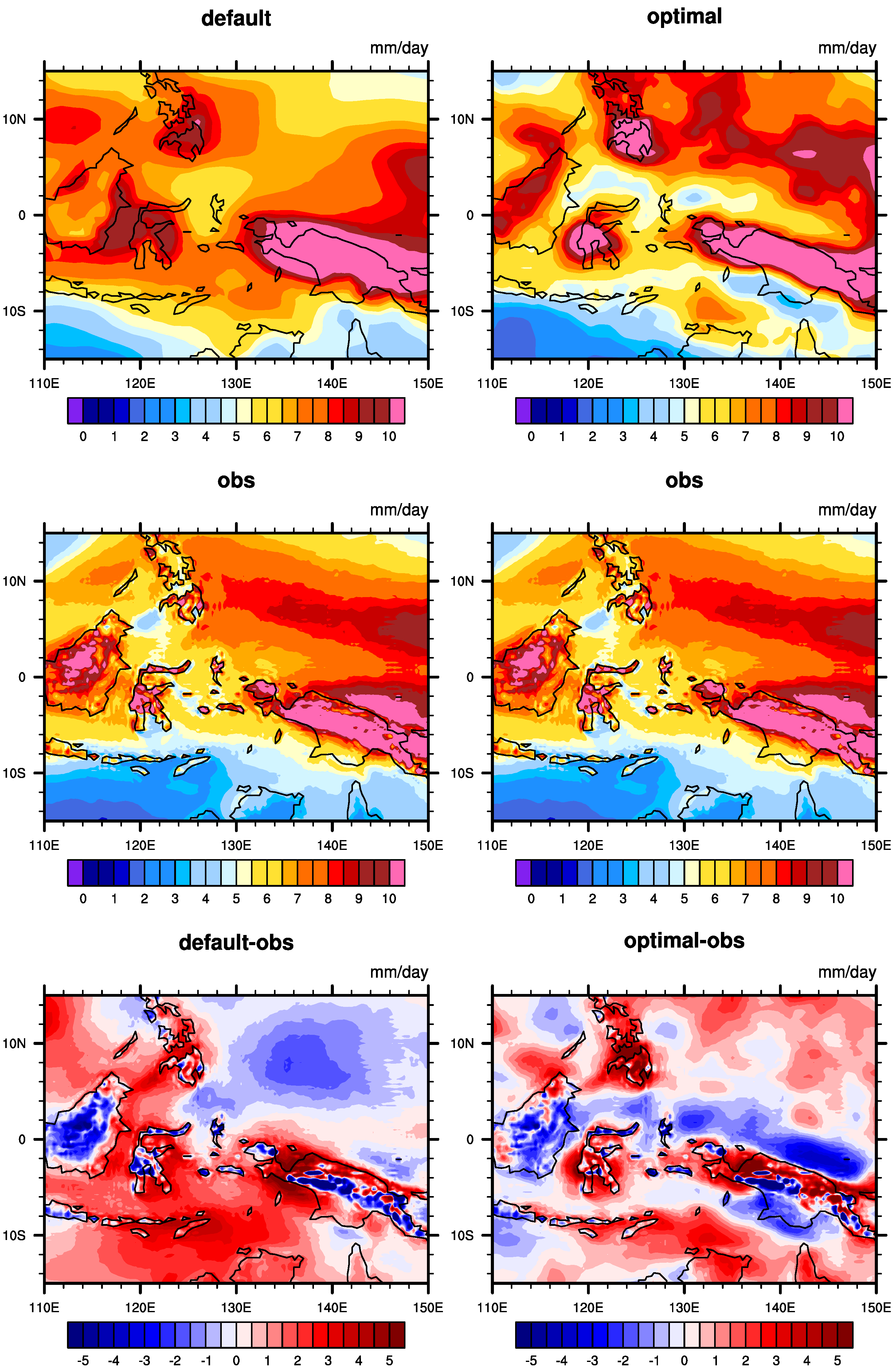
Compared with several other optimization areas, the Warm Pool area spans multiple longitude and latitude ranges, the oceans and continents are intertwined, and the precipitation is relatively large but the optimization results are still positive in many areas. In the southern area near ${10}^{\circ }$S, there is a phenomenon of heavy precipitation inconsistent with the observed data in the default experiment. The optimized results in Figure 11 and Figure S9 show that the precipitation in these areas has been effectively weakened in the model simulation, and the result is closer to the observation data. This improvement can be clearly shown in the xy plot of the zonal mean in Figure 10b. Furthermore, the problem of negative precipitation bias in the default simulation over Sulawesi Island (near $5^{\circ }$S and ${120}^{\circ }$E) has been reduced, and the regions centered on the island have been positively changed. The improvement in the Northern Hemisphere is mainly concentrated in the areas of $4^{\circ }$–${10}^{\circ }$N and ${130}^{\circ }$–${150}^{\circ }$E. The precipitation intensity of the default simulation in this area is far less than the observation data, and the optimization experiment increases the precipitation in this area. The situation of excessive precipitation in the northwest of the Warm Pool has also been improved to a certain extent in the optimization experiment. However, in areas poleward of ${10}^{\circ }$N, the simulation results of the optimization experiment are not ideal, which also makes the deviation in the corresponding areas in the XY plot of the zonal mean larger and leads to an insufficient improvement in the RMSE. Nevertheless, for the Warm Pool, the optimization results still reflect changes that are consistent with the observations.

The xy plot of the zonal mean of South Asia is shown in Figure 10c, and it can be seen that the variation in precipitation with latitude has completely changed after optimization compared with the default simulation. The overall precipitation in the default experiment increases with latitude, while after optimization, it decreases, aligning with the reanalysis data. The optimized values are closer to the reanalysis data compared to the default simulation. The precipitation distribution of the default simulation and optimization result are shown in Figure 12. Compared with the default simulation, ocean precipitation is increased over western Indonesia so that the negative error is almost eliminated, and it is decreased over ${105}^{\circ }$–${120}^{\circ }$E. For land precipitation, the changes are smaller than for ocean precipitation, and there also exist differences in magnitude. Figure S13 depicts the precipitation changes across different regions of South Asia. Overall, precipitation has increased in the southwestern part compared to the default experiment, while the northeastern region shows lower precipitation values than in the default experiment. However, the error between simulation and observation is significantly reduced.

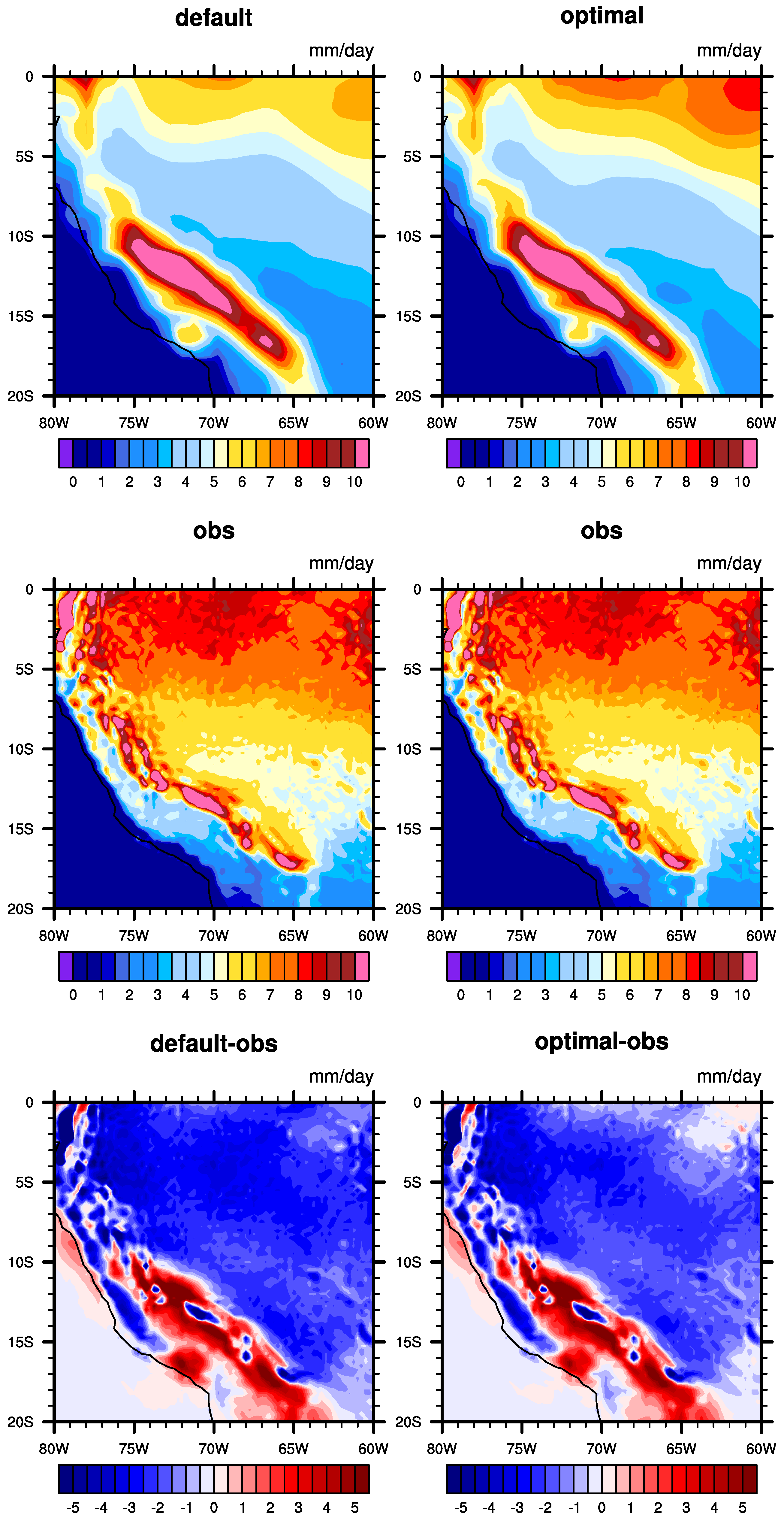
In the default simulation of the Nino region (Figure 13), the observation inconsistency is mainly concentrated in two areas, the negative error area on the western side and the positive error area on the eastern side of the selected domain. For the improvement and optimization results of these two areas, there are obvious heavy rainfall centers; the positive error area is basically consistent with the observation data, and the negative error area is also reduced. The central region with a large error generated by the default experiment still exists after optimization but the value is closer to that of the observation data than of the default result. On the whole, this shows a positive optimization; however, in the xy plot of the meridional mean in Figure 10d, the precipitation over the high-value area in the optimization result is lower than in the observation. Due to the small latitudinal range of the region, we considered analyzing the variation in precipitation with longitude. Figure 13 shows the curve of precipitation variation with longitude in the Nino region. It can be seen that precipitation in the western area has increased compared to in the default experiment, while it has decreased in the eastern area. However, in most of the optimized areas, the results are closer to the reanalysis data. Figure S11 more clearly illustrates the different trends on both sides of the region. The reason is that when improving the area of positive difference, a new small part of the negative error is introduced from the area east of ${100}^{\circ }$W, which is the reason for the large difference in the zonal mean between the simulation and default values.

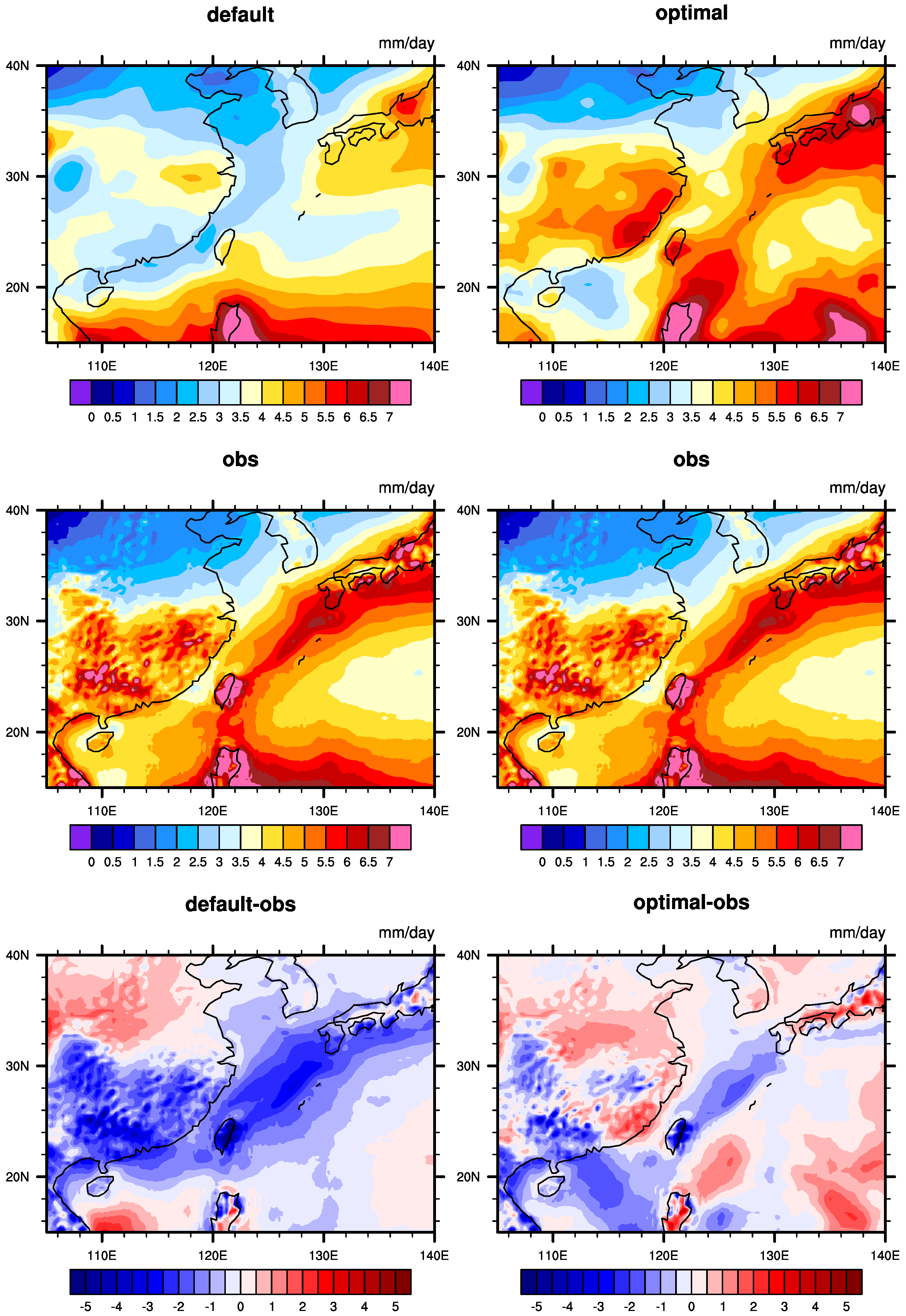
The results in East Asia are similar to those in South Asia, which are shown in Figure 14. In East Asia, the precipitation of the default experiment is generally less than that of the reanalysis data, with the discrepancy being more pronounced in southern China and the Huanghai Sea region. We can see that in the default experiment, there is a relatively large error over the Donghai Sea, centered around the area between Taiwan and Japan, even extending to the Huanghai Sea, the Sea of Japan, and the Korean Peninsula. The optimization results suggest that this error is almost eliminated over these regions, and it is also markedly reduced over the central area. The same is true in southern China. Precipitation in southern China is increased after parameter optimization, which is low in default simulation and hard to match with observations. Figure S14 shows that compared to the default experiment, the optimized CAM precipitation values have increased across most of the East Asia region. In addition, other areas are also improved to different degrees, such as central China and the South China Sea. We observe such positive changes using the xy plot of the zonal mean (Figure 10e), which demonstrates that the optimization result is better than that of the default simulation in most cases, especially at ${20}^{\circ }$N–${30}^{\circ }$N, which corresponds to the changes over southern China and the Donghai Sea.

As shown in Figure 15, the characteristics of the precipitation in South America are wide-ranging and high in quantity, and it is difficult to obtain results consistent with the observations. Compared with the default, the optimized results reflect precipitation changes that are more consistent with the observations in some areas. The zonal mean (Figure 10f) shows that the optimization result has better performance at ${12}^{\circ }$S–$2^{\circ }$N, and the spatial distribution shows that a small area at approximately ${65}^{\circ }$W–${60}^{\circ }$W near the south of the equator has improved after a parameter optimization. Even so, there is a great difference between the model simulation and the observation when evaluating South America. And Figure S12 shows that the difference between the default experiment and the optimized experiment is not as significant as in the other regions. Overall, the optimization effect is not significant.

The impact of parameters on precipitation is not entirely linear; it may even exhibit drastic oscillations. The effects on a global scale can be quite different from those on a regional scale. Therefore, for parameter tuning in precipitation simulations, efficient methods are crucial. Apart from expert knowledge, it is essential to have a rapid approach for exploring the parameter space and finding optimal solutions with limited computational resources. The method we proposed in this paper, based on a multilevel surrogate model, leverages the advantages of surrogate models in iteration and computing the objective function, enabling a swift search within the parameter space to identify superior solutions. The increase in these parameters is the main reason for the increase in precipitation.

3.3. Ensemble Optimization Results of the Nonuniform Parameter Parameterization Scheme

In the local optimization experiments, we found that a local optimization may lead to the simulation results of other regions moving in a worse direction; that is, the optimization of one region is at the cost of worse results in other regions, which is unacceptable. Therefore, we designed a nonuniform parameter parameterization scheme to integrate the optimal parameters of multiple regions into one case. In the selected region, we use the parameters obtained through the surrogate model-based optimization methods and use default values in other regions. To prevent the large difference in parameter values between the two sides of the regional boundary from affecting the experimental results, we designed a boundary smoothing scheme to achieve a smooth transition of parameter values from the center to the boundary of each region. The same or similar parameter values are obtained at the boundary:

$$\begin{array}{cc}\hfill & x=max(\left|{\displaystyle \frac{lat-centerlat}{\frac{1}{2}width}}\right|,\left|{\displaystyle \frac{lon-centerlon}{\frac{1}{2}length}}\right|)\hfill \end{array}$$

(5)

$$\begin{array}{cc}\hfill & weight={\displaystyle \frac{1}{2}}(cos\left(\pi x^3\right)+1)\hfill \end{array}$$

(6)

$$\begin{array}{cc}\hfill & value=(optmization\_value-default\_value)\ast weight+default\_value\hfill \end{array}$$

(7)

where x is used to evaluate the distance from each point in the region to the center of the region. $lat,lon$ represent the latitude and longitude of the point, respectively, and $centerlat,centerlon$ represent the latitude and longitude of the center point. $width,length$ represent the width and length of the selected region. The denominator is equal to the distance between two boundaries and the center point. x means the maximum distance from the point to the length or width of the region, and the value is between 0 and 1. $weight$ is the weight of the distance for each point. The closer to the center point, the closer the weight is to 1, and the closer the parameter value is to the optimized value. The closer to the boundary, the closer the weight is to 0, and the closer the parameter value is to the default value. Equation (7) provides a cosine weight function that allows each real number between 0 and 1 to correspond to a 0–1 variation interval, and the dependent variable gradually decreases as the independent variable increases.

The ensemble parameter experiment results are shown in

Table 5. The tuning results of the ensemble parameter experiment over a selected region.

Region	Default RMSE	Optimized RMSE	Better (+) or Worse (−)
Warm Pool	1.985	2.037	-
South Pacific	0.855	0.802	+
Nino	0.931	0.741	+
South America	2.576	2.540	+
South Asia	1.521	1.759	-
East Asia	1.213	1.054	+

. In this case, different parameters were set according to different regions, and out of the six regions, four regions achieved better simulation results than the default experiment, with two regions performing slightly worse than the default experiment. We know that the simulation results of each region are, to some extent, influenced by the parameter values of other regions, so it is difficult to achieve a level of individual optimization for each region in Section 3.2. Among them, the South Pacific, Nino, South America, and East Asia regions all achieved varying degrees of improvement, while the results of the Warm Pool and South Asia regions slightly decreased compared to the default values. The distribution map of precipitation is shown in Figure 16. Compared with the default experiment, the new experimental results have undergone many positive changes; precipitation in North China was reduced, and precipitation in the East China Sea and the ocean area east of the East China Sea increased, which are the reasons for the improvement of the simulation results over East Asia. In the Pacific region, a portion of the precipitation within the ${150}^{\circ }$W–${120}^{\circ }$W, ${20}^{\circ }$–${30}^{\circ }$S region was reduced; however, there was an increase in precipitation in the western region and near the equator, which also resulted in the simulation results in the South Pacific region not being as significant as the regional optimization results in Section 3.2. The precipitation levels in the Nino region located in the eastern Pacific Ocean near Central America are reduced, and the improvements in some areas to the west are all positive. On the South American continent, some small-scale increases in precipitation are the reason for improving the simulation effect in South America, as such areas are relatively small, so the overall improvement is not significant. In addition, in regions such as Southern Africa, Central Asia, and the Gulf of Mexico, precipitation decreases to varying degrees compared to the default experiments. However, the increase in precipitation in the Warm Pool and South Asian regions result in a slight increase in error between the simulation results and the default experiment. Overall, the results of such simulation experiments can reach a level close to that in the default experiment in most regions, with relatively positive changes in some regions, and only a small portion of the results are slightly lower than the level of the default experiment. Beyond the selected regions in this study, other areas also show varying degrees of improvement. For example, there is a reduction in precipitation near the Cuban islands and the Gulf of Mexico, precipitation suppression in the northeastern part of the Australian islands, and slightly better precipitation performance in the North Pacific around ${180}^{\circ }$W–${150}^{\circ }$W compared to the default experiment, as well as improvements in southern Africa’s precipitation. These regions within ${30}^{\circ }$N–${30}^{\circ }$S have all seen varying levels of precipitation enhancement.

3.4. Evaluation of Simulation Results Related to Precipitation Using Remote Sensing Data

To further elucidate the results of parameter tuning and the nonuniform parameter parameterization scheme, we introduce comparisons with other metrics. Given that our approach is a single-objective parameter optimization method and cannot simultaneously optimize multiple objective metrics. We aimed to demonstrate, by examining the variations in other metrics, that our method improved precipitation without introducing significant errors in other aspects. We used remote sensing data for analyzing these variables because, compared to reanalysis data, remote sensing data directly reflect the actual conditions of the Earth’s surface, making them more intuitive. We selected relative humidity (RELHUM), Top of Atmosphere (TOA), Upward Longwave Flux (FLUT), and Temerature (T). The observations of the RELHUM and T were from an Atmospheric Infrared Sounder (AIRS) Pagano et al. [54], and FLUT, from an Earth Radiation Budget Experiment (ERBE) Barkstrom [55].

Pressure–latitude distributions of the RELHUM are shown in Figures S3 and S4. Combining the results from the simulation experiments and the differences with remote sensing data, we find that the changes between the two sets of experiments are not significant. Under the majority of pressure and latitude conditions, there is hardly any noticeable difference between the two datasets. Only in a very few latitude regions, such as the $0^{\circ }$–${20}^{\circ }$S area at 400 mb and the vicinity of ${40}^{\circ }$N at 500 mb, do we observe extremely subtle differences. In summary, compared to the default parameter experiment, the optimized experiment shows no significant change in relative humidity (RELHUM).

As can be seen in Figures S5 and S6, the optimized experiment and the default experiment show consistent simulation results for temperature (T) across different pressures and latitudes. Figure 1 and Figure 2 indicate that, except for extremely minor differences at a few specific altitudes and latitudes, there are virtually no significant discrepancies. This suggests that, despite improvements in precipitation, there has been no significant change to the temperature simulation. The simulation results for T in the optimized experiment continue to be on par with those of the default experiment.

The spatial distribution of FLUT is shown in Figures S7 and S8. The simulation results of T850 obtained from the nonuniform parameterization scheme experiment, similar to the simulation results for relative humidity (RELHUM) and temperature (T) experiments with the nonuniform parameterization scheme, maintain a high level of consistency with the default experiment in most areas. Comparisons with reanalysis data show slight improvements in the simulation over the default experiment in regions like East Asia and the Indian Ocean. However, in areas such as the South Pacific and North Atlantic, the default experiment performs slightly better results. In terms of mean and extreme values, the simulation results of both experiments are very close. Overall, the simulation values remain at the same level.

The reasons for this situation are believed to be primarily the following. First, the parameters chosen for optimization specifically target precipitation sensitivity and may not be as sensitive to other metrics, hence the limited impact on these metrics. Second, in this study, the compset selected utilizes climatological sea surface temperature (SST) data for ocean simulation. If CMIP-related compsets with variable SST data were employed, it is possible that more variations could be observed. In conclusion, our proposed optimization method based on a multilevel surrogate model and the nonuniform parameterization scheme, while optimizing precipitation simulation results, does not introduce significant errors in other metrics.

4. Summary and Conclusions

The surrogate model is widely used to solve complex and expensive optimization problems, such as various Earth system models, and it has not received enough attention in CAM5 parameter optimization. In this paper, we proposed a multilevel surrogate model-based parameter optimization method for CAM5 precipitation. First, we demonstrated that the surrogate model method can be used to improve the precipitation simulation of CAM5. An appropriate surrogate model was selected by cross validation. Second, we proposed a multilevel surrogate method, which was demonstrated to have a faster convergence speed and fewer errors during the tuning process. Third, because of the “rocker” effect of the parameter, we designed region-based optimization experiments and selected six regions as the performance indicators. The improvement was more pronounced in the South Pacific and East Asia regions, reaching 46.78% and 27.68%, respectively. The improvement in the Nino and South Asia regions also increased by about 15%. The two regions with a more modest improvement were the Warm Pool and South America regions, which were both below 10% at 3.07% and 7.94%, respectively. To integrate these results over each region, we attempted a nonuniform parameter parameterization scheme and implemented weight-based boundary smoothing for each region. In the new parameterization scheme, the same parameter has different values in different regions. The optimal parameters of the six regions were integrated into one case over the corresponding region. The ensemble parameter experimental results show positive changes in four of the six regions we selected, but two regions did not improve. This also reflects certain limitations in the CAM5 surrogate model-based optimization.

The main highlights of this study are as follows:

1. We first proposed a surrogate model-based parameter tuning method for CAM5 precipitation in this study. In considering that the nonlinearity and complexity of CAM5 are much higher than those of other models, the effectiveness and feasibility of the method were validated in this work.

2. We designed a multilevel surrogate model. The multilevel surrogate model integrates the candidate point approach (CAND) and trust region to update the surrogate model in each iteration. The results show that the proposed method has a faster convergence speed and fewer errors during the tuning process. We designed a nonuniform parameter parameterization scheme and integrated parameters using a parameter smoothing scheme.

3. We explored the influence of the same parameter on precipitation over different regions. Then, a region-based optimization method was proposed based on this result, and we constructed different surrogate models for each area. The average improvement of the selected regions was 19%. The nonuniform parameter parameterization scheme attempts simultaneous optimizations for as many regions as possible, and the experimental results were improved in four regions.

In future work, we will continue to explore the application of surrogate models and the nonuniform parameter parameterization scheme for parameter tuning in CAM5, including combinations with other methods, such as AI-based prediction techniques, to build more accurate surrogate models for CAM. Additionally, we will integrate variable resolution Wills et al. [56] with the nonuniform parameter parameterization scheme using variable-resolution grids in tuning regions. Furthermore, we plan to apply this method to other variables or conduct multi-objective optimizations to identify parameter combinations that can effectively improve the simulation performance of multiple variables.

References

1. Williams, P.D. Modelling climate change: The role of unresolved processes. Philos. Trans. R. Soc. A Math. Phys. Eng. Sci. 2005, 363, 2931–2946. [Google Scholar] [CrossRef] [PubMed]
2. Hack, J.; Boville, B.; Kiehl, J.; Rasch, P.; Williamson, D. Climate statistics from the National Center for Atmospheric Research community climate model CCM2. J. Geophys. Res. Atmos. 1994, 99, 20785–20813. [Google Scholar] [CrossRef]
3. Bauer, P.; Thorpe, A.; Brunet, G. The quiet revolution of numerical weather prediction. Nature 2015, 525, 47–55. [Google Scholar] [CrossRef] [PubMed]
4. Mastrandrea, M.D.; Mach, K.J.; Plattner, G.K.; Edenhofer, O.; Stocker, T.F.; Field, C.B.; Ebi, K.L.; Matschoss, P.R. The IPCC AR5 guidance note on consistent treatment of uncertainties: A common approach across the working groups. Clim. Change 2011, 108, 675–691. [Google Scholar] [CrossRef]
5. Wu, L.; Zhang, T.; Qin, Y.; Xue, W. An effective parameter optimization with radiation balance constraint in CAM5 (version 5.3). Geosci. Model Dev. 2020, 13, 41–53. [Google Scholar] [CrossRef]
6. Yang, B.; Qian, Y.; Lin, G.; Leung, L.R.; Rasch, P.J.; Zhang, G.J.; McFarlane, S.A.; Zhao, C.; Zhang, Y.; Wang, H.; et al. Uncertainty quantification and parameter tuning in the CAM5 Zhang-McFarlane convection scheme and impact of improved convection on the global circulation and climate. J. Geophys. Res. Atmos. 2013, 118, 395–415. [Google Scholar] [CrossRef]
7. Liang, F.; Cheng, Y.; Lin, G. Simulated stochastic approximation annealing for global optimization with a square-root cooling schedule. J. Am. Stat. Assoc. 2014, 109, 847–863. [Google Scholar] [CrossRef]
8. Hourdin, F.; Williamson, D.; Rio, C.; Couvreux, F.; Roehrig, R.; Villefranque, N.; Musat, I.; Fairhead, L.; Diallo, F.B.; Volodina, V. Process-based climate model development harnessing machine learning: II. Model calibration from single column to global. J. Adv. Model. Earth Syst. 2021, 13, e2020MS002225. [Google Scholar] [CrossRef]
9. Couvreux, F.; Hourdin, F.; Williamson, D.; Roehrig, R.; Volodina, V.; Villefranque, N.; Rio, C.; Audouin, O.; Salter, J.; Bazile, E.; et al. Process-based climate model development harnessing machine learning: I. A calibration tool for parameterization improvement. J. Adv. Model. Earth Syst. 2021, 13, e2020MS002217. [Google Scholar] [CrossRef]
10. Villefranque, N.; Blanco, S.; Couvreux, F.; Fournier, R.; Gautrais, J.; Hogan, R.J.; Hourdin, F.; Volodina, V.; Williamson, D. Process-based climate model development harnessing machine learning: III. The representation of cumulus geometry and their 3D radiative effects. J. Adv. Model. Earth Syst. 2021, 13, e2020MS002423. [Google Scholar] [CrossRef]
11. Zhang, T.; Li, L.; Lin, Y.; Xue, W.; Xie, F.; Xu, H.; Huang, X. An automatic and effective parameter optimization method for model tuning. Geosci. Model Dev. 2015, 8, 3579–3591. [Google Scholar] [CrossRef]
12. Williamson, D.; Goldstein, M.; Allison, L.; Blaker, A.; Challenor, P.; Jackson, L.; Yamazaki, K. History matching for exploring and reducing climate model parameter space using observations and a large perturbed physics ensemble. Clim. Dyn. 2013, 41, 1703–1729. [Google Scholar] [CrossRef]
13. Williamson, D.; Blaker, A.T.; Hampton, C.; Salter, J. Identifying and removing structural biases in climate models with history matching. Clim. Dyn. 2015, 45, 1299–1324. [Google Scholar] [CrossRef]
14. Williamson, D.B.; Blaker, A.T.; Sinha, B. Tuning without over-tuning: Parametric uncertainty quantification for the NEMO ocean model. Geosci. Model Dev. 2017, 10, 1789–1816. [Google Scholar] [CrossRef]
15. Zhang, T.; Zhang, M.; Lin, W.; Lin, Y.; Xue, W.; Yu, H.; He, J.; Xin, X.; Ma, H.Y.; Xie, S.; et al. Automatic tuning of the Community Atmospheric Model (CAM5) by using short-term hindcasts with an improved downhill simplex optimization method. Geosci. Model Dev. 2018, 11, 5189–5201. [Google Scholar] [CrossRef]
16. Gilewski, P. Application of global environmental multiscale (GEM) numerical weather prediction (NWP) model for hydrological modeling in mountainous environment. Atmosphere 2022, 13, 1348. [Google Scholar] [CrossRef]
17. Sun, C.; Jin, Y.; Cheng, R.; Ding, J.; Zeng, J. Surrogate-Assisted Cooperative Swarm Optimization of High-Dimensional Expensive Problems. IEEE Trans. Evol. Comput. 2017, 21, 644–660. [Google Scholar] [CrossRef]
18. Lian, Y.; Liou, M.S. Multiobjective Optimization Using Coupled Response Surface Model and Evolutionary Algorithm. AIAA J. 2005, 43, 1316–1325. [Google Scholar] [CrossRef]
19. Vapnik, V. The Nature of Statistical Learning Theory; Springer Science & Business Media: Berlin/Heidelberg, Germany, 1999. [Google Scholar]
20. Loshchilov, I.; Schoenauer, M.; Sebag, M. A Mono Surrogate for Multiobjective Optimization. In Proceedings of the 12th Annual Conference on Genetic and Evolutionary Computation, GECCO ’10, Portland, OR, USA, 7–11 July 2010; pp. 471–478. [Google Scholar] [CrossRef]
21. Gutmann, H.M. A radial basis function method for global optimization. J. Glob. Optim. 2001, 19, 201–227. [Google Scholar] [CrossRef]
22. Gaspar-Cunha, A.; Vieira, A. A multi-objective evolutionary algorithm using neural networks to approximate fitness evaluations. Int. J. Comput. Syst. Signals 2005, 6, 18–36. [Google Scholar]
23. Rasmussen, C.E. Gaussian processes in machine learning. In Summer School on Machine Learning; Springer: Berlin/Heidelberg, Germany, 2003; pp. 63–71. [Google Scholar]
24. Jie, H.; Wu, Y.; Zhao, J.; Ding, J.; Liangliang. An efficient multi-objective PSO algorithm assisted by Kriging metamodel for expensive black-box problems. J. Glob. Optim. 2017, 67, 399–423. [Google Scholar] [CrossRef]
25. Neelin, J.D.; Bracco, A.; Luo, H.; McWilliams, J.C.; Meyerson, J.E. Considerations for parameter optimization and sensitivity in climate models. Proc. Natl. Acad. Sci. USA 2010, 107, 21349–21354. [Google Scholar] [CrossRef] [PubMed]
26. Müller, J.; Paudel, R.; Shoemaker, C.A.; Woodbury, J.; Wang, Y.; Mahowald, N. CH4 parameter estimation in CLM4.5bgc using surrogate global optimization. Geosci. Model Dev. 2015, 8, 3285–3310. [Google Scholar] [CrossRef]
27. Xu, H.; Zhang, T.; Luo, Y.; Huang, X.; Xue, W. Parameter calibration in global soil carbon models using surrogate-based optimization. Geosci. Model Dev. 2018, 11, 3027–3044. [Google Scholar] [CrossRef]
28. Wang, C.; Duan, Q.; Gong, W.; Ye, A.; Di, Z.; Miao, C. An evaluation of adaptive surrogate modeling based optimization with two benchmark problems. Environ. Model. Softw. 2014, 60, 167–179. [Google Scholar] [CrossRef]
29. Gong, W.; Duan, Q.; Li, J.; Wang, C.; Di, Z.; Dai, Y.; Ye, A.; Miao, C. Multi-objective parameter optimization of common land model using adaptive surrogate modeling. Hydrol. Earth Syst. Sci. 2015, 19, 2409–2425. [Google Scholar] [CrossRef]
30. Di, Z.; Duan, Q.; Wang, C.; Ye, A.; Miao, C.; Gong, W. Assessing the applicability of WRF optimal parameters under the different precipitation simulations in the Greater Beijing Area. Clim. Dyn. 2018, 50, 1927–1948. [Google Scholar] [CrossRef]
31. Chinta, S.; Balaji, C. Calibration of WRF model parameters using multiobjective adaptive surrogate model-based optimization to improve the prediction of the Indian summer monsoon. Clim. Dyn. 2020, 55, 631–650. [Google Scholar] [CrossRef]
32. Zhang, C.; Di, Z.; Duan, Q.; Xie, Z.; Gong, W. Improved Land Evapotranspiration Simulation of the Community Land Model Using a Surrogate-Based Automatic Parameter Optimization Method. Water 2020, 12, 943. [Google Scholar] [CrossRef]
33. Qian, Y.; Yan, H.; Hou, Z.; Johannesson, G.; Klein, S.; Lucas, D.; Neale, R.; Rasch, P.; Swiler, L.; Tannahill, J.; et al. Parametric sensitivity analysis of precipitation at global and local scales in the Community Atmosphere Model CAM5. J. Adv. Model. Earth Syst. 2015, 7, 382–411. [Google Scholar] [CrossRef]
34. Chen, D.; Dai, A. Precipitation characteristics in the Community Atmosphere Model and their dependence on model physics and resolution. J. Adv. Model. Earth Syst. 2019, 11, 2352–2374. [Google Scholar] [CrossRef]
35. Li, J.; Yu, R.; Yuan, W.; Chen, H.; Sun, W.; Zhang, Y. Precipitation over E ast A sia simulated by NCAR CAM5 at different horizontal resolutions. J. Adv. Model. Earth Syst. 2015, 7, 774–790. [Google Scholar] [CrossRef]
36. Pathak, R.; Sahany, S.; Mishra, S.K. Impact of Stochastic Entrainment in the NCAR CAM Deep Convection Parameterization on the Simulation of South Asian Summer Monsoon. Clim. Dyn. 2021, 57, 3365–3384. [Google Scholar] [CrossRef]
37. Wang, Y.; Zhang, G.J.; Craig, G.C. Stochastic convective parameterization improving the simulation of tropical precipitation variability in the NCAR CAM5. Geophys. Res. Lett. 2016, 43, 6612–6619. [Google Scholar] [CrossRef]
38. Cui, Z.; Zhang, G.J.; Wang, Y.; Xie, S. Understanding the roles of convective trigger functions in the diurnal cycle of precipitation in the NCAR CAM5. J. Clim. 2021, 34, 6473–6489. [Google Scholar] [CrossRef]
39. Wang, Y.; Zhang, G.J. Global climate impacts of stochastic deep convection parameterization in the NCAR CAM 5. J. Adv. Model. Earth Syst. 2016, 8, 1641–1656. [Google Scholar] [CrossRef]
40. Dennis, J.M.; Edwards, J.; Evans, K.J.; Guba, O.; Lauritzen, P.H.; Mirin, A.A.; St-Cyr, A.; Taylor, M.A.; Worley, P.H. CAM-SE: A scalable spectral element dynamical core for the Community Atmosphere Model. Int. J. High Perform. Comput. Appl. 2012, 26, 74–89. [Google Scholar] [CrossRef]
41. Adler, R.F.; Sapiano, M.R.; Huffman, G.J.; Wang, J.J.; Gu, G.; Bolvin, D.; Chiu, L.; Schneider, U.; Becker, A.; Nelkin, E.; et al. The Global Precipitation Climatology Project (GPCP) monthly analysis (new version 2.3) and a review of 2017 global precipitation. Atmosphere 2018, 9, 138. [Google Scholar] [CrossRef]
42. Hersbach, H.; Bell, B.; Berrisford, P.; Hirahara, S.; Horányi, A.; Muñoz-Sabater, J.; Nicolas, J.; Peubey, C.; Radu, R.; Schepers, D.; et al. The ERA5 global reanalysis. Q. J. R. Meteorol. Soc. 2020, 146, 1999–2049. [Google Scholar] [CrossRef]
43. Pathak, R.; Sahany, S.; Mishra, S.K. Uncertainty quantification based cloud parameterization sensitivity analysis in the NCAR community atmosphere model. Sci. Rep. 2020, 10, 17499. [Google Scholar] [CrossRef]
44. Sanderson, B.M.; Piani, C.; Ingram, W.; Stone, D.; Allen, M. Towards constraining climate sensitivity by linear analysis of feedback patterns in thousands of perturbed-physics GCM simulations. Clim. Dyn. 2008, 30, 175–190. [Google Scholar] [CrossRef]
45. Abdulkareem, J.; Pradhan, B.; Sulaiman, W.; Jamil, N. Review of studies on hydrological modelling in Malaysia. Model. Earth Syst. Environ. 2018, 4, 1577–1605. [Google Scholar] [CrossRef]
46. Stisen, S.; Jensen, K.H.; Sandholt, I.; Grimes, D.I. A remote sensing driven distributed hydrological model of the Senegal River basin. J. Hydrol. 2008, 354, 131–148. [Google Scholar] [CrossRef]
47. Iman, R.L.; Helton, J.C.; Campbell, J.E. An approach to sensitivity analysis of computer models: Part I—Introduction, input variable selection and preliminary variable assessment. J. Qual. Technol. 1981, 13, 174–183. [Google Scholar] [CrossRef]
48. Regis, R.G.; Shoemaker, C.A. A stochastic radial basis function method for the global optimization of expensive functions. INFORMS J. Comput. 2007, 19, 497–509. [Google Scholar] [CrossRef]
49. Browne, M.W. Cross-validation methods. J. Math. Psychol. 2000, 44, 108–132. [Google Scholar] [CrossRef]
50. MacKay, D.J. Introduction to Gaussian processes. NATO ASI Ser. F Comput. Syst. Sci. 1998, 168, 133–166. [Google Scholar]
51. Karim, L.R.; Ellaia, R.; Talbi, E.G. Kriging-Based Multi-objective Infill Criterion using NSGA-III for Expensive Black-Box Functions. In Proceedings of the 2020 5th International Conference on Logistics Operations Management (GOL), Virtual, 28–30 October 2020; IEEE: Piscataway, NJ, USA, 2020; pp. 1–10. [Google Scholar]
52. Garrido-Merchán, E.C.; Hernández-Lobato, D. Dealing with categorical and integer-valued variables in bayesian optimization with gaussian processes. Neurocomputing 2020, 380, 20–35. [Google Scholar] [CrossRef]
53. Xie, S.; Zhang, M.; Boyle, J.S.; Cederwall, R.T.; Potter, G.L.; Lin, W. Impact of a revised convective triggering mechanism on Community Atmosphere Model, Version 2, simulations: Results from short-range weather forecasts. J. Geophys. Res. Atmos. 2004, 109, D14. [Google Scholar] [CrossRef]
54. Pagano, T.S.; Aumann, H.H.; Hagan, D.E.; Overoye, K. Prelaunch and in-flight radiometric calibration of the Atmospheric Infrared Sounder (AIRS). IEEE Trans. Geosci. Remote Sens. 2003, 41, 265–273. [Google Scholar] [CrossRef]
55. Barkstrom, B.R. The earth radiation budget experiment (ERBE). Bull. Am. Meteorol. Soc. 1984, 65, 1170–1185. [Google Scholar] [CrossRef]
56. Wills, R.C.; Herrington, A.R.; Simpson, I.R.; Battisti, D.S. Resolving weather fronts increases the large-scale circulation response to Gulf Stream SST anomalies in variable-resolution CESM2 simulations. J. Adv. Model. Earth Syst. 2024, 16, e2023MS004123. [Google Scholar] [CrossRef]
Figure 1. Regions selected in this study. In the figure, 1–6 represent East Asia, South Asia, Warmpool, Nino, South Pacific, and South America, respectively.
Remotesensing 17 00408 g001
Figure 2. Flowchart of multilevel surrogate model-based parameter tuning method.
Remotesensing 17 00408 g002
Figure 3. Cross-validation results comparing the performances of these methods. The Y-axis represents the relative error between the experimental and reanalysis data.
Remotesensing 17 00408 g003
Figure 4. Cross-validation results of bottom-level surrogate model construction methods.
Remotesensing 17 00408 g004
Figure 5. The tuning process with the proposed multilevel surrogate model-based method and ASMO method, and the corresponding relative error of these two methods, where the relative error is equal to ( | p r e d i c t v a l u e r e a l v a l u e | ) / r e a l v a l u e .
Remotesensing 17 00408 g005
Figure 6. Comparison of different methods with default as baseline.
Remotesensing 17 00408 g006
Figure 7. The average error during the optimization iteration process.
Remotesensing 17 00408 g007
Figure 8. The symbolic consistency of rhminl disturbance and corresponding precipitation change.
Remotesensing 17 00408 g008
Figure 9. The precipitation distribution of the South Pacific optimization results. The left column shows the default simulation, observation data, and difference between the default simulation and observation data from top to bottom. The right column shows the optimal experiment data, observation data, and the difference between the optimal experiment and the observation data from top to bottom.
Remotesensing 17 00408 g009
Figure 10. The xy plot of the zonal mean of precipitation over selected regions (meridional mean in (d)); the X-axis shows the latitude (longitude in (d)), and the Y-axis represents the precipitation value. The blue, red, and black lines represent the optimal experiment, the default simulation, and the observation data, respectively.
Remotesensing 17 00408 g010
Figure 11. The precipitation distribution of the Warm Pool optimization results. The left column shows the default simulation, observation data and the difference between the default simulation and the observation data from top to bottom. The right column shows the optimal experiment data, observation data, and the difference between the optimal experiment and observation data from top to bottom.
Remotesensing 17 00408 g011
Figure 12. The precipitation distribution of the South Asia optimization results. The left column shows the default simulation data, observation data, and the difference between the default simulation and the observation data from top to bottom. The right column shows the optimal experiment data, observation data, and the difference between the optimal experiment and the observation data from top to bottom.
Remotesensing 17 00408 g012
Figure 13. The precipitation distribution of the Nino optimization results. The left column shows the default simulation data, observation data, and the difference between the default simulation and the observation data from top to bottom. The right column shows the optimal experiment data, observation data, and the difference between the optimal experiment and the observation data from top to bottom.
Remotesensing 17 00408 g013
Figure 14. The precipitation distribution of the East Asia optimization results. The left column shows the default simulation data, observation data, and the difference between the default simulation and the observation data from top to bottom. The right column shows the optimal experiment data, observation data, and the difference between the optimal experiment and the observation data from top to bottom.
Remotesensing 17 00408 g014
Figure 15. The precipitation distribution of the South America optimization results. The left column shows the default simulation data, observation data, and the difference between the default simulation and the observation data from top to bottom. The right column shows the optimal experiment data, observation data, and the difference between the optimal experiment and the observation data from top to bottom.
Remotesensing 17 00408 g015
Figure 16. The difference between the experiment simulation results with the ensemble parameters of each region and the default experiment simulation results.
Remotesensing 17 00408 g016