Enhancing Long-Term Flood Forecasting with SageFormer: A Cascaded Dimensionality Reduction Approach Based on Satellite-Derived Data

Abstract

Floods, increasingly exacerbated by climate change, are among the most destructive natural disasters globally, necessitating advancements in long-term forecasting to improve risk management. Traditional models struggle with the complex dependencies of hydroclimatic variables and environmental conditions, thus limiting their reliability. This study introduces a novel framework for enhancing flood forecasting accuracy by integrating geo-spatiotemporal analyses, cascading dimensionality reduction, and SageFormer-based multi-step-ahead predictions. The framework efficiently processes satellite-derived data, addressing the curse of dimensionality and focusing on critical long-range spatiotemporal dependencies. SageFormer captures inter- and intra-dependencies within a compressed feature space, making it particularly effective for long-term forecasting. Performance evaluations against LSTM, Transformer, and Informer across three data fusion scenarios reveal substantial improvements in forecasting accuracy, especially in data-scarce basins. The integration of hydroclimate data with attention-based networks and dimensionality reduction demonstrates significant advancements over traditional approaches. The proposed framework combines cascading dimensionality reduction with advanced deep learning, enhancing both interpretability and precision in capturing complex dependencies. By offering a straightforward and reliable approach, this study advances remote sensing applications in hydrological modeling, providing a robust tool for mitigating the impacts of hydroclimatic extremes.

1. Introduction

Water scarcity continues to be one of the most significant challenges facing sedentary societies because of the non-uniform spatial and temporal distributions of precipitation [1,2]. Moreover, these uneven distributions of precipitation cause natural disasters such as floods and droughts, which are exacerbated in severity and frequency by anthropogenic factors such as urbanization, climate change, population, and economic growth [3,4,5,6,7,8]. Indeed, UNICEF has highlighted that climate change is exacerbating water-related hazards because rising temperatures are disrupting precipitation patterns as well as the entire water cycle [9]. Therefore, proactive flood management is necessary not only to enhance resilience to drought and water scarcity but also to transform these threats into opportunities for increased profitability.

Proactive flood management undertakes long-term forecasting of complex hydrological events using earth system modeling (ESM). Flood prediction through ESM has evolved to encompass physical models grounded in physical processes, conceptual models that abstract these processes, and data-driven techniques that have emerged with increasing data availability [10,11,12,13]. These methodologies range from rainfall-runoff modeling and univariate streamflow prediction to multivariate models that consider hydroclimate data to capture complex nonlinear spatiotemporal dependencies [14,15,16]. Because the countries that most need ESM are typically the least prepared to employ it in terms of available data and expertise, the use of spatiotemporal models and satellite data has emerged as a valuable approach for conducting ESM to aid flood forecasting.

The successful application of deep learning (DL) models for handling geo-spatiotemporal data has been the subject of extensive research in hydrological forecasting [17,18,19,20,21,22,23,24]. Convolutional neural networks (CNNs) have traditionally been employed for this purpose due to their effectiveness in capturing local patterns and spatial dependencies within gridded data [22]. However, a significant limitation of CNNs lies in their inability to efficiently process complex spatiotemporal data with numerous non-value grids. This inefficiency arises because CNNs are designed for regular grid structures, leading to high computational costs when handling large, heterogeneous datasets often encountered in hydroclimatic modeling. Previous studies have explored the use of global hydroclimate data to enhance the accuracy of streamflow prediction through spatiotemporal modeling. For instance, Ghobadi and Kang [15] utilized mesoscale hydroclimate data as additional predictors to improve the performance of an innovative neural network architecture integrating CNN for extracting geo-spatiotemporal features with a Transformer-based attention network for multi-step-ahead streamflow prediction. However, they reported high computational costs associated with the CNN, even when the inputs were limited by selecting only the most highly correlated grids, and highlighted challenges related to overfitting owing to the large volume and short duration of the available data, which exacerbated the curse of dimensionality. A similar attempt by Li et al. [25] indicated the potential of attention-based Transformer networks for enhancing flood forecasting accuracy. Perera et al. [26] used a combination of anthropogenic, static physiographic, and dynamic climate variables as inputs for a modified generative adversarial network-based model to predict streamflow. In contrast, graph neural networks (GNNs) offer a more flexible approach by representing data as a graph of interconnected nodes, where each node corresponds to a spatial location (grid) and edges represent spatial or temporal dependencies [27]. This graph-based representation allows GNNs to effectively model the irregular and complex relationships between hydroclimatic variables without being restricted to a fixed grid structure [28]. GNNs inherently capture both local and global dependencies, making them more suitable for handling data that exhibit strong interconnectivity between adjacent and non-adjacent grids. By transforming spatial grids into graph nodes, GNNs can address the limitations of CNNs in dealing with the irregularities and heterogeneity of geo-spatiotemporal data. However, the increased flexibility of GNNs comes at the cost of higher computational complexity, particularly when dealing with a large number of nodes. The computational burden is exacerbated in scenarios involving extensive hydroclimatic datasets, where redundant nodes may introduce noise and unnecessary complexity. This necessitates an efficient data preprocessing step to reduce the dimensionality of the input data while preserving critical information.

Considering the increase in model complexity, as datasets have become voluminous and ubiquitous, Ghobadi et al. [16] utilized a dimensionality reduction (DR) technique coupled with an attention-based informer network for long-term multi-step-ahead streamflow prediction to extract key information from a dataset and eliminate less informative variables. A recent study proposed a novel series-aware graph-enhanced Transformer model called SageFormer that not only captures temporal dependencies but also eliminates redundant information across the input series; it was shown to be capable of modeling both intra- and inter-series dependencies in long-term multivariate time series forecasting [29]. This framework amalgamates GNN with a Transformer structure to enrich the model’s ability to comprehend complex interdependencies.

Recent advances in attention-based architectures and GNNs have shown considerable promise for capturing spatiotemporal correlations in long-term multivariate time series forecasting [29]. However, to the best of the authors’ knowledge, the application of cutting-edge series-aware algorithms to address complex spatiotemporal dependencies and learning efficiency to achieve robust long-term forecasting remains an ongoing challenge in the field of hydrology. Therefore, the objective of this study was to address these research gaps by investigating the application of the cutting-edge SageFormer modeling method and comparing its predictive abilities with those of established Transformer-based methods when integrated with DR techniques to demonstrate its performance in long-term flood forecasting. This research is expected to contribute to sustainable development by informing proactive strategies for mitigating and adapting to flooding, particularly in developing countries that require data fusion to inform predictions.

The primary objective of this study is to address the research gaps mentioned earlier. The novelties of this study are fourfold. First, it introduces an innovative multi-step-ahead flood forecasting framework designed to enhance predictive accuracy for long-term flood forecasting while mitigating the curse of dimensionality. Second, it proposes a cascade dimensionality reduction technique for geo-spatiotemporal data fusion to utilize complex datasets as booster variables efficiently. The cascade DR process systematically eliminates redundant nodes by compressing the feature space and reducing the number of non-essential dependencies. To the best of the authors’ knowledge, this is the first application of a multi-step-ahead, multivariate SageFormer-based model in hydrology, introducing a state-of-the-art attention-based algorithm capable of effectively capturing inter- and intra-dependencies within multivariate time series data. As an additional contribution, this study conducts a comprehensive comparative analysis of a conventional LSTM alongside three advanced attention-based algorithms—Transformer, Informer, and SageFormer—highlighting their performance in diverse data fusion scenarios and underscoring SageFormer’s potential as a transformative tool for hydrological applications.

The remainder of this paper is organized as follows: Section 2 presents the materials and methods, comprising an overview of the Transformer (Section 2.1), a discussion of the application of SageFormer to hydroclimate modeling (Section 2.2), a description of the proposed framework (Section 2.3), details of the case study and data acquisition methods (Section 2.4), and the definitions of the performance evaluation metrics (Section 2.5) and experimental settings (Section 2.6) employed; the results and discussion are presented in Section 3; and the conclusions drawn from the results are presented in Section 4 along with directions for future research.

2. Materials and Methods

This section provides a concise overview of the general Transformer and cutting-edge SageFormer architecture, details the data acquisition methods and study framework, and defines the applied case study.

2.1. Overview of Transformer Architecture

The Transformer architecture represents a significant advancement in sequence modeling that departs from traditional recurrent and convolutional approaches in favor of a fully attention-based mechanism, as described by Vaswani et al. [30]. It employs an encoder–decoder structure that effectively leverages parallel computations to optimize the use of modern graphics processing units (GPUs). In contrast to recurrent neural networks (NNs), which process data sequentially, Transformer processes input sequences in parallel using unique components, including multi-head self-attention mechanisms and positionally encoded embeddings, that allow the model to simultaneously capture the global dependencies between inputs and outputs [15].

In the Transformer workflow, the embedded input data first undergo positional encoding to retain temporal sequence information [30]. The core of the Transformer, the multi-head attention mechanism, processes these data by analyzing and weighting interactions across different positions within the sequence. This mechanism processes sets of query, key, and value vectors through multiple attention heads to calculate similarity weights, thereby facilitating a comprehensive understanding of sequence dependencies [30]. The output from this attention process is further refined by feedforward NNs with residual connections, enhancing training stability and enabling the model to capture complex dependencies within the data. The ability of the Transformer architecture to handle sequences in parallel, combined with its efficient use of attention to model interactions and dependencies, makes it a powerful tool for handling a broad range of sequence-based tasks in a computationally efficient manner.

2.2. SageFormer for Hydroclimate Modeling

SageFormer leverages a series-aware framework enhanced with a GNN and the Transformer architecture [29]. This approach excels at capturing the complex long-term inter-series dependencies inherent in multivariate hydrological data, which are crucial when forecasting phenomena such as streamflow and flood events over extended periods. The integrated GNN allows SageFormer to map the intricate relationships between various hydrological variables, producing a nuanced understanding of spatial and temporal patterns [29]. The Transformer component, which is equipped with multi-head attention mechanisms, allows SageFormer to efficiently process large datasets to discern critical temporal dynamics [29]. As a result, the SageFormer model not only improves long-term forecasting accuracy by handling both intra- and inter-series interactions but also adapts to the nonlinear and dynamic nature of hydroclimate processes, offering substantial improvements over traditional forecasting models [29]. This makes SageFormer an innovative tool in the hydroclimate research domain, where accurate long-term forecasting is pivotal for effective water resources management and disaster mitigation strategies.

In the SageFormer architecture, $x_{t }\in {\mathbb{R}}^C$ indicates the value of series $C$ at time step t, given a historical multivariate time series $X_t=\left[x_t, x_{t+1},\dots , x_{t+H-1}\right]\in {\mathbb{R}}^{C\times H}$ with a duration H, and the goal is to forecast the next T steps of the multivariate time series $Y_t=\left[x_{t+L},\dots , x_{t+L+T-1}\right]\in {\mathbb{R}}^{C\times T}$ [29]. A GNN is employed to represent inter-series dependencies in a multivariate time series by considering different series as nodes and describing the interdependencies among them using a graph adjacency matrix. The SageFormer workflow consists of two basic components: global token generation and iterative message passing. Compared to conventional Transformer-based models, SageFormer introduces a pivotal contribution by integrating global tokens inspired by the class tokens employed in natural language processing models and vision Transformer. These global tokens are used to effectively capture intra-series temporal dependencies; interested readers are referred to Zhang et al. [29] for further details. The graph structure learning module in SageFormer can be described as follows [29]:

$$M_1=\mathrm{a}\mathrm{c}\mathrm{t}\left({\rm E}{\mathsf{\Theta }}_1\right); M_2=\mathrm{a}\mathrm{c}\mathrm{t}\left({\rm E}{\mathsf{\Theta }}_2\right),$$

(1)

$$\acute{A}=\mathrm{R}\mathrm{e}\mathrm{l}\mathrm{u}\left(M_1{M_2}^T-M_2{M_1}^T\right),$$

(2)

in which series node embedding is learned by the random initialization of ${\rm E}\in {\mathbb{R}}^{C\times D_g}$, where $D_g$ represents the number of features in node embeddings, and the nonlinear activation function “$\mathrm{a}\mathrm{c}\mathrm{t}$” uses the trainable parameters ${\mathsf{\Theta }}_1$ and ${\mathsf{\Theta }}_2$ to transform ${\rm E}$ into $M\in {\mathbb{R}}^{C\times D_g}$; subsequently, the top $K$ nearest nodes are identified as neighbors to $\acute{A}$ and the unconnected nodes are set to zero. As implemented in the original study [29], Relu was utilized as the activation function in this study to ensure nonlinearity and effectively learn meaningful embeddings.

The SageFormer encoder layers, in which graph aggregation and temporal encoding are performed iteratively, process the embedding tokens to disseminate the global information gathered by the GNN. This iterative message passing allows the model to effectively capture both intra- and inter-series dependencies. As illustrated in the fifth block of Figure 1a, each series fuses its information with that of its neighbors through graph aggregation, thereby enhancing the series representation by incorporating related patterns. For each series in the $l$th layer, the first $M$ embeddings take the global tokens of layer $l$ as $G_i^{\left(l\right)}\leftarrow {\chi }_{:,i,:}^{\left(l\right)}\in {\mathbb{R}}^{C\times D}, i\le M.$ As illustrated in the lower section of the fifth block in Figure 1a, the global tokens of layer $l$ are collected from all series and then fed as input into the GNN for graph aggregation using multi-hop information fusion on the graph as follows [29]:

$${\widehat{G}}_i={\sum }_{d=0}^D{\tilde{A}}^d{G}_i{W}_d, i\le M,$$

(3)

where $D$ represents the graph aggregation depth, $\tilde{A}$ represents the graph Laplacian matrix, and $W_d\in {\mathbb{R}}^{D\times D}$ defines the set of learnable parameters. These matrices adjust and scale the hydroclimate feature vectors at each graph layer, enabling the model to effectively capture and integrate information across various neighborhood scales. Each embedding ${\widehat{G}}_i$ is returned to its original series and concatenated with the series tokens, resulting in graph-enhanced embeddings ${\widehat{\chi }}^{\left(l\right)}$.

These graph-enhanced embeddings are subsequently processed using Transformer components. Vanilla Transformer encoder blocks are employed as the foundational architecture [29], and the outputs from these blocks serve as token-level embeddings for the subsequent encoding layer. The information previously aggregated by the GNN is distributed across other tokens within each series through self-attention, allowing access to the relevant series data. This approach significantly enhances the expressiveness of the model compared with that of a series-independent model. Both node embeddings and global tokens are randomly initialized and optimized through iterative message passing, similar to GNN graph aggregation techniques. The input tensors share the format $(b, n, d)$, representing the batch size, number of nodes, and feature dimensions, respectively. The initial temporal encoding ensures that global tokens carry comprehensive information, enhancing the convergence of the model during graph aggregation.

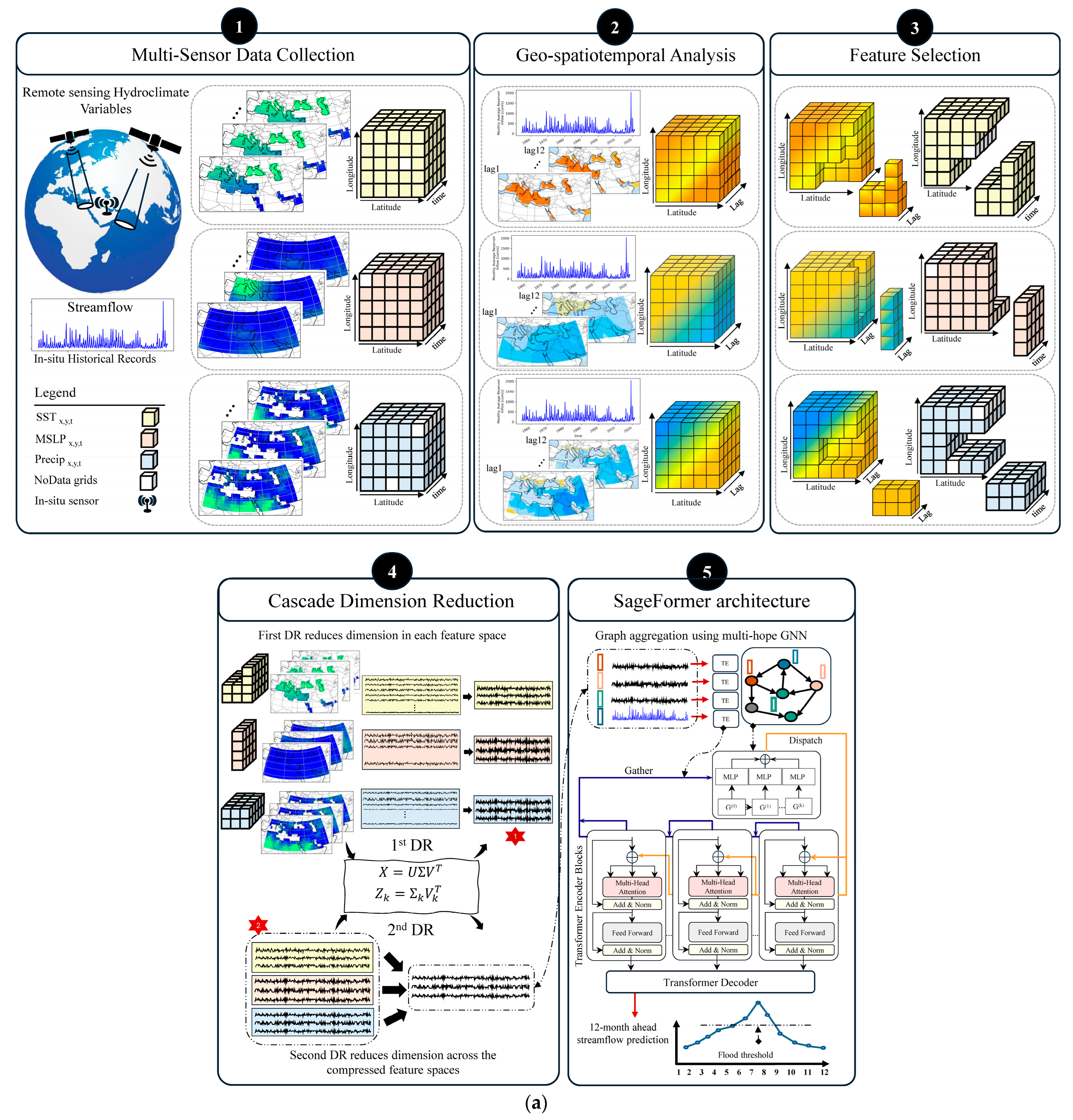
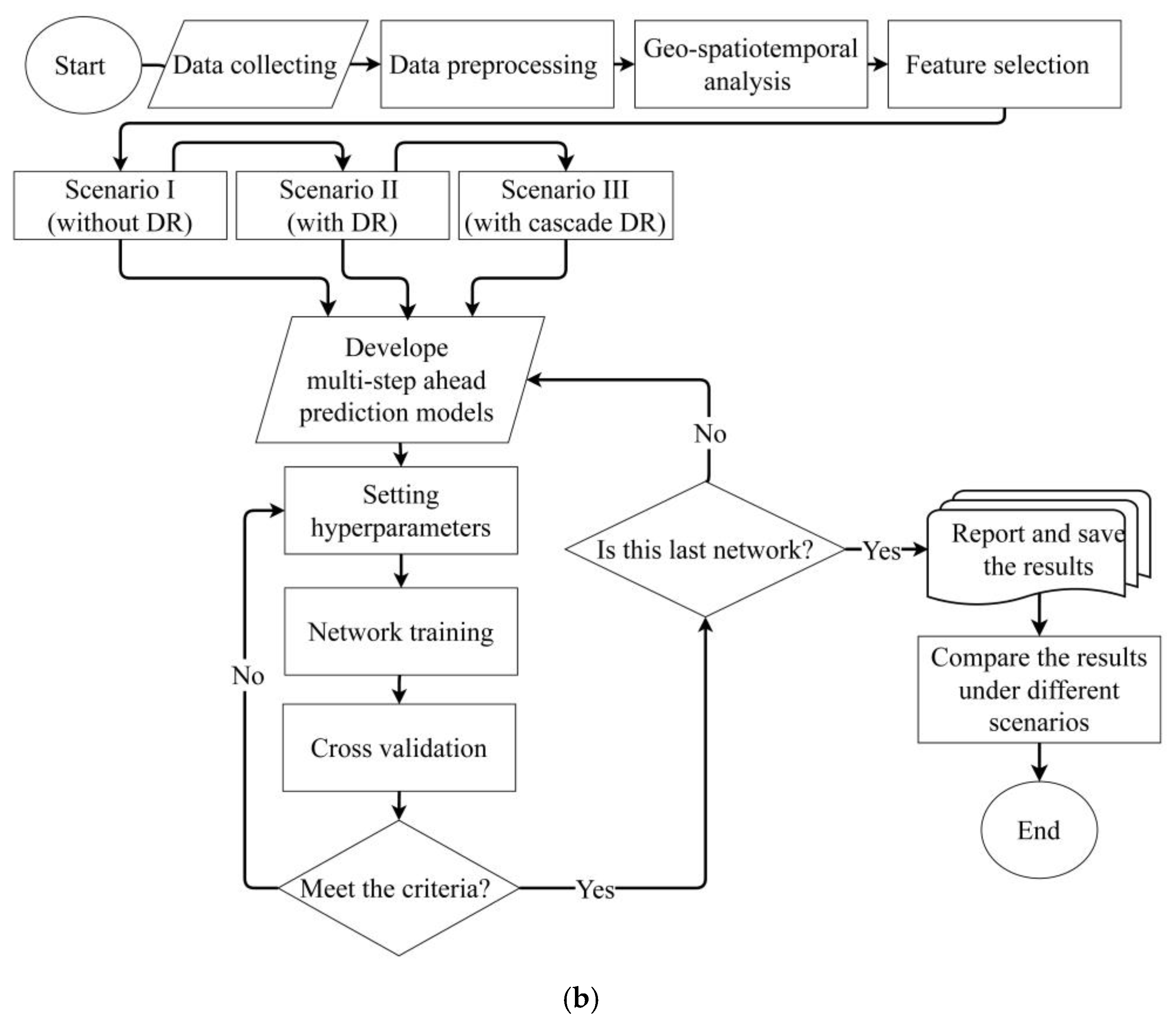
2.3. Proposed Framework

In our previous study [8], innovative methods such as three-dimensional CNNs and time-distributed CNNs were utilized to perform automatic feature engineering. These techniques focus on extracting highly correlated grids for the same features and subsequently processing them using the DR technique. It is worth mentioning that a major drawback of using CNNs for hydroclimate data in a geo-spatiotemporal structure is the high computational cost, primarily due to the processing of numerous non-value grids. Further research has expanded the application of DR to multivariate time series data. This progression underscores the evolving methodology for handling complex spatial and temporal data to refine feature extraction and enhance model performance in predictive analytics [31]. Therefore, this study evaluated the efficacy of different preprocessing strategies for handling high-dimensional geospatial data within the context of neural network-based forecasting models.

Initially, this study explored a scenario in which spatial grids were identified through correlation analysis and filtered using predefined thresholds. The selected grids were directly employed as independent features in the model without any DR. This approach, referred to as Scenario I, served as a baseline to assess the impact of raw data on model performance. In contrast, Scenario II applied principal component analysis (PCA) as a DR technique to the same filtered grids for each feature to enhance model efficiency by reducing data complexity and noise. This DR process strove to maintain 95% of the variance in the original dataset when selecting the optimal number of components, thereby ensuring that the most significant features were preserved and mitigating the curse of dimensionality often encountered in high-dimensional datasets. To further expand the analysis, Scenario III employed a novel approach in which the output features from the initial DR, which retained the critical variance of the original data, were aggregated and subjected to a second round of DR. This cascading DR process was designed to further refine the feature set and potentially uncover more abstract relationships and patterns that were not apparent in the initial reduction phase. This implementation of the cascading DR approach probed the ability of layered feature compression to enhance the predictive capabilities of the model. The steps discussed earlier are illustrated in Figure 1a, while the study’s logical flowchart is shown in Figure 1b. The datasets used in this study include sea surface temperature (SST), mean sea level pressure (MSLP), and precipitation (Precip). These datasets are visually represented in Figure 1a, with yellow denoting SST, orange representing MSLP, and blue indicating Precip. A detailed explanation of these datasets and their preprocessing is provided in Section 2.4.

These preprocessing strategies were rigorously evaluated using three cutting-edge (NN) architectures: the Transformer [30], known for its robust handling of sequential data via attention mechanisms; the Informer [32], which extends the Transformer’s capabilities using efficient long-range dependency modeling; and SageFormer [29], a recent innovation that incorporates a GNN to exploit inter- and intra-series dependencies more effectively. The use of a “vanilla” long short-term memory (Vanilla LSTM) model was also evaluated as a baseline model. The performance of each model was quantified in terms of its ability to handle the processed data and extract meaningful insights, providing a comprehensive understanding of the interplay between data preprocessing and advanced neural computation techniques in forecasting scenarios. This approach not only demonstrated the adaptability and effectiveness of each model under different data preprocessing scenarios but also illuminated the path towards more sophisticated data integration strategies in NN frameworks.

2.4. Case Study Basin and Data Acquisition

The study framework was applied to the Karkheh River basin in southwest Iran, which spans 50,800 km² and encompasses five sub-basins. This region features diverse topography, ranging from plains to mountains, leading to complex hydrological characteristics. Furthermore, it experiences a Mediterranean climate with wet winters and dry summers, and its annual precipitation varies from 300 mm in the south to 800 mm in the north. The Karkheh Dam became operational in 2002 and is primarily intended for flood control and agricultural water supply; northern snowmelt and Mediterranean airflow serve as the major water sources for its reservoir.

This study utilized the monthly streamflow time series obtained at the location of the Karkheh Reservoir from 1955 to 2021 as field-measured data. As shown in Figure 2, the study domain encompassed from 20°N to 45°N and from 0°E to 60°E were selected based on the rationale presented in the literature [15]. Three mesoscale monthly gridded datasets were utilized: precipitation (Precip), sea surface temperature (SST), and mean sea level pressure (MSLP) with spatial resolution accuracies of 2.5° × 2.5°, 2° × 2°, and 2.5° × 2.5°, respectively. Linear interpolation was employed to obtain a homogenous spatial resolution of 2° × 2° among all features. The SST and MSLP datasets were derived from the International Comprehensive Ocean-Atmosphere Dataset Release 3.0 [33], and the Precip dataset was obtained from the Global Precipitation Climatology Center [34]. Figure 3 presents a sample of satellite-derived input data, illustrating the scaled values of the three gridded input features over 12 months.

2.5. Performance Evaluation Metrics

This study adopted a combination of indicators to validate the forecasting performances of the considered models beyond the capabilities of the conventional built-in fit statistics, using the mean absolute error (MAE) and mean square error (MSE) to quantify the badness-of-fit and the coefficient of determination (R²) and Pearson correlation coefficient to quantify the goodness-of-fit.

2.6. Experimental Settings

Before the model training was initiated, the field-measured data were preprocessed using standardization by removing the mean and scaling to unit variance and log transformation to enhance learning speed and convergence. These steps comprised part of the initial phase of model development. To demonstrate the superiority of SageFormer as a series-aware framework compared to the two other attention-based networks (Informer and Transformer), their performance was also compared with that of Vanilla LSTM. The MSE was employed as the objective function for validation because of its effectiveness in penalizing larger errors, which is crucial for accurately representing extreme hydrological events such as floods [14,35,36].

The data were divided into three segments: the first segment comprised 85% of the data (spanning from 1955 to 2010) and was used to train the model; the second and third segments together comprised the remaining 15%, with the data from 2010 to 2015 used for validation and that from 2015 to 2020 used for testing. A sliding window approach with a window size of 12 months was applied, incorporating a retrospective input and a batch size of 12 months to effectively replicate the annual conditions relevant to multi-step-ahead forecasting for the following year. The prediction models were developed using Python 3.6.9 and implemented on an NVIDIA^® GeForce^® RTX 4090 GPU with an Intel^® Core i9-10920X processor operating at 3.5 GHz and 128 GB of memory.

3. Results

This section first illustrates geo-spatiotemporal feature selection using the Pearson correlation. Next, time series feature extraction through DR is discussed, and the performance of the three attention-based deep learning algorithms is compared with that of Vanilla LSTM under the three scenarios defined in Section 2.3 to demonstrate the performance of the cutting-edge SageFormer network.

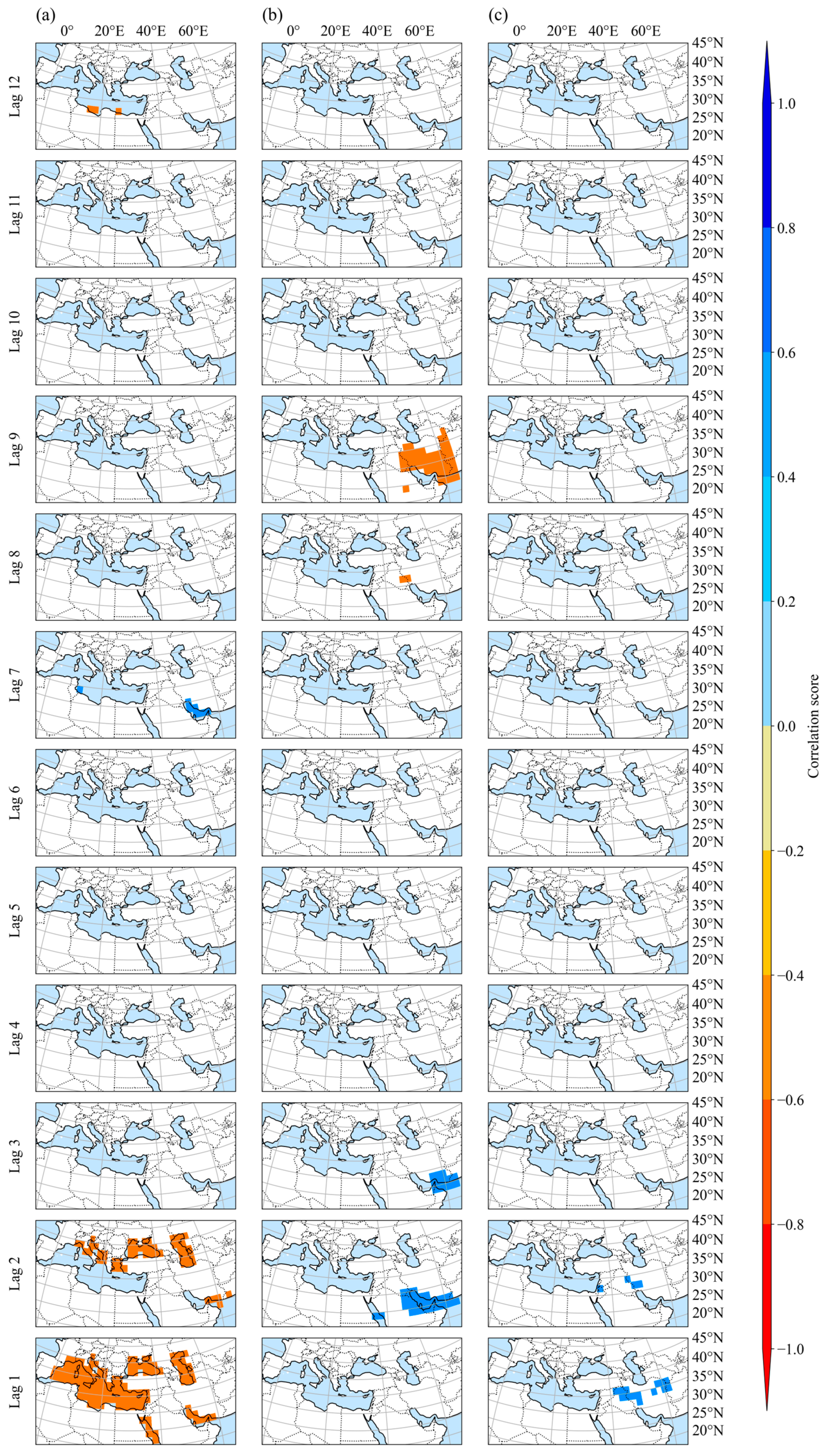
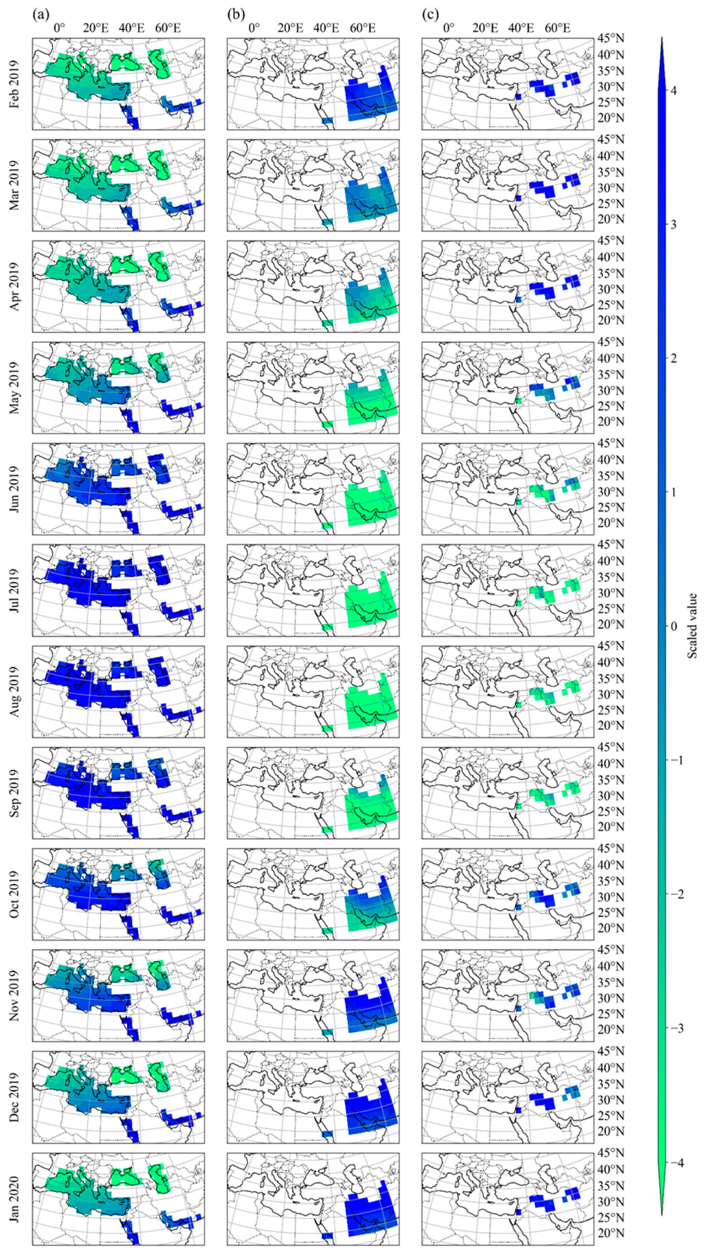
3.1. Geo-Spatiotemporal Data Feature Selection

The geo-spatiotemporal correlations between the SST, MSLP, and Precip datasets and the field-measured streamflow across lags 1 to 12 are depicted in Figure 4a–c, respectively. According to the geo-spatiotemporal correlation analysis among SST and streamflow presented in Figure 4a, the SST data exhibited the highest absolute correlation coefficient, with the field-measured streamflow of approximately 0.8 at lags 1, 2, 7, and 12, followed by a correlation coefficient of 0.6 at lags 3 and 6. The correlation values vary over time, showing negative correlations at lags 1 to 4, positive correlations at lags 5 to 9, and a return to negative correlations at lags 10 to 12. The regions with the strongest correlations between SST and streamflow include the Persian Gulf, Caspian Sea, and Mediterranean Sea. According to Figure 4a, SST correlation values exhibit a spatial gradient from east to west. A similar spatial pattern is observed for MSLP correlations, as shown in Figure 4b. As shown in Figure 4b, the correlation values fluctuate across the lags, showing positive correlations at lags 1 to 5, negative correlations at lags 6 to 11, and reverting to negative correlations at lag 12. In the case of Precip, as shown in Figure 4c, the correlation results exhibit a more localized, centric pattern. Areas adjacent to the study region demonstrate the highest absolute correlation values, with significant positive correlations observed at lags 1 and 2, and negative correlations at lags 8 and 9. As shown in Figure 4c, correlation changes, both positive and negative, are present across all lags among Precip and streamflow. The geo-spatiotemporal correlation analysis highlights the varying spatial and temporal relationships between the input features and streamflow. The correlation scores were used to optimally select booster variables considering lagged effects and spatial heterogeneity in the modeling process.

The maximum correlation results using Pearson and Spearman’s rank-order correlation for a 12-month lag among SST, MSLP, and Precip with streamflow are presented in Figure 5a–c, respectively. The final subplot (Figure 5d) shows the autocorrelation of streamflow, indicating that data from the preceding 12 months should be utilized in the model to predict the subsequent 12 months. As shown in Figure 5, there is a slight difference between the Pearson and Spearman rank-order correlation results, particularly for highly correlated values. Consequently, the Pearson correlation results were used for identifying the highly correlated grids.

Highly correlated regions with a Pearson correlation coefficient greater than 0.7 were identified using a predefined threshold filter, with the results shown in Figure 6a–c for the SST, MSLP, and Precip datasets, respectively. As shown in Figure 6a, when a threshold filter of 0.70 was applied to the SST data, all sea grids within the selected study domain demonstrated a significant correlation with streamflow at lags 1 and 2. The correlation results for the MSLP data, shown in Figure 6b, indicated a maximum absolute correlation coefficient of 0.8 at lags 2, 3, 8, and 9, with the most correlated grids situated adjacent to the Karkheh River and the Persian Gulf. Considering the established link between atmospheric circulation and river flow noted by Kingston et al. [37], the geographic and climatic diversity of Iran clearly influences its precipitation patterns. Therefore, detailed analyses of the correlations between endogenous and exogenous variables must be performed to identify grids with high correlations [15]. Finally, the Precip data exhibited its highest positive correlation coefficient of 0.6 adjacent to the case study area at lags 1 and 2, as shown in Figure 6c. The results, based on the union of the highly correlated grids identified through the geo-spatiotemporal correlation analysis and used as inputs to the SageFormer model, are presented in Figure 7a–c for the SST, MSLP, and Precip, respectively. Due to the capability of the predictive model employed in this study, there is no need to select different grids for each lag. This approach not only reduces the curse of dimensionality but also fully leverages the strengths of SageFormer as an attention-based prediction model, which is well suited for capturing complex spatiotemporal dependencies and relationships in the data.

3.2. Flood Forecasting Model Evaluation

Three different preprocessing scenarios were evaluated to determine the effects of input on the flood forecasting performance of models varying in complexity from Vanilla LSTM to the more sophisticated architectures of the Transformer, Informer, and series-aware SageFormer, which leverages both Transformer and GNN technologies to capture intricate intra- and inter-series dependencies. The first scenario used all grids with SST, MSLP, and Precip dataset correlation coefficients higher than 0.7 as independent variables in the forecasting model (Scenario I); the second scenario passed the selected high-correlation grids and their high-correlation lags through DR to reduce the computational cost, generating a new time series as an input to proceed with the prediction while maintaining 95% of the variance in the original dataset (Scenario II); finally, the third scenario subjected the features output from the initial DR in Scenario II to a second round of DR (Scenario III). This not only alleviates the computational load on the GNN but also enhances the model’s ability to focus on meaningful spatiotemporal patterns. To further substantiate the computational cost, the training time across the scenarios was evaluated. SageFormer achieved an average running time of 0.53 ± 0.03 s per batch in Scenario I, 0.42 ± 0.05 s per batch in Scenario II, and 0.36 ± 0.02 s per batch in Scenario III. These results demonstrate the effectiveness of cascading DR in significantly reducing computational overhead while maintaining predictive performance.

Scatter plots of the forecasted and observed monthly streamflow for all models under the three scenarios are shown in Figure 8, which indicates that the least scattered and most accurate flood event predictions were provided by the SageFormer model under Scenario III. Although the disparity among all models is evident, it can primarily be attributed to the nature of multi-step-ahead forecasting, which inherently introduces cumulative errors. This issue is especially pronounced in autoregressive models, as errors are propagated and amplified over successive prediction steps. The superior performance of SageFormer can be attributed to its integrated approach, which combines the strengths of the attention mechanisms in the Transformer with the capacity of the GNN to process complex network structures. This dual approach enabled the SageFormer model to effectively parse and learn from both temporal sequences and spatial relationships within the data, which is critical for predicting phenomena with spatial disparities and temporal variances, such as floods.

The most pronounced improvement in performance from Scenario I to III was observed in the SageFormer model, followed by the Informer and Transformer models, highlighting the efficiency of these attention-based models in leveraging cascading DR and the superior ability of their sophisticated architectures to handle complex spatiotemporal data dependencies compared to purely temporal models, such as Vanilla LSTM. These results emphasize the advanced capabilities of SageFormer in handling the challenges posed by flood forecasting. In particular, its ability to integrate and analyze complex data structures makes it a valuable tool in hydrology, as this can provide insights informing effective flood management strategies. Thus, the results demonstrate not only the model’s technical proficiency but also its potential contribution to enhancing resilience and sustainability in flood-prone regions, especially in developing countries where available data may be limited. This aligns with the broader goals of sustainable development by reducing disaster risk and enhancing adaptive capacity at multiple levels.

Note that all models except SageFormer consistently underestimated the peak flood values, whereas SageFormer accurately forecast the values of these chaotic natural phenomena. This excellent performance can be particularly advantageous for flood management preparedness, especially in sensitive areas, as it allows for a more conservative approach to planning and response strategies. Conservative planning can potentially reduce the risk of catastrophic outcomes in scenarios where underestimation could lead to insufficient preparedness. The performance of each model across all scenarios, assessed in terms of the MAE, MSE, R², and Pearson correlation coefficient, is summarized in

Table 1. Comparison of model performance when 12-step-ahead forecasting.

Model	MAE	MSE	R2	Pearson Correlation
Scenario I
Vanilla LSTM	0.776	0.874	0.234	0.714
Transformer	0.712	0.830	0.272	0.589
Informer	0.712	0.824	0.277	0.593
SageFormer	0.539	0.467	0.590	0.791
Scenario II
Vanilla LSTM	0.685	0.689	0.396	0.748
Transformer	0.677	0.727	0.363	0.685
Informer	0.591	0.604	0.470	0.730
SageFormer	0.482	0.360	0.685	0.833
Scenario III
Vanilla LSTM	0.685	0.735	0.355	0.687
Transformer	0.598	0.627	0.450	0.730
Informer	0.523	0.487	0.573	0.782
SageFormer	0.481	0.387	0.661	0.822

. These metrics describe the accuracy, reliability, and correlation of each model’s predictions with the field-measured outcomes.

As shown in Table 1, the SageFormer model outperformed the other models in all scenarios, exhibiting the lowest MAE and MSE as well as the highest R² and Pearson correlation values. This superior performance indicates its robust ability to extract and leverage the essential features of geo-spatiotemporal datasets, even at this basic level of data preprocessing, with its accompanying curse of dimensionality. Scenario II introduced a higher level of data preprocessing by applying DR directly to the feature-selected grids. As shown in Table 1, all models in this scenario demonstrated improvements in terms of MAE, MSE, R², and Pearson correlation. This aligns with previous findings regarding the impact of DR on forecasting performance [31,38]. The results obtained in this scenario underscore the importance of applying DR to selected grids to enhance the accuracy of a complex model, particularly when using SageFormer, which benefits from the ability of the GNN to capture intricate patterns within the data. Conversely, the simpler recurrent NN of Vanilla LSTM struggled to capture inter-series and long-term dependencies, leading to a deterioration in performance from Scenarios II to III. Indeed, as an inherently temporal model without advanced feature extraction capabilities, LSTM fails to effectively capture complex inter-series dependencies. According to Table 1, the Vanilla LSTM model exhibited the weakest performance, with the highest MSE values of 0.735 in Scenario III and 0.689 in Scenario II. However, from Scenarios I to II, its performance improved in terms of MSE, R², and Pearson correlation, which aligns with the findings of Ghobadi et al. [31] regarding the impact of DR on forecasting performance. These results suggest that cascading DR exacerbates performance issues associated with temporal models, such as Vanilla LSTM, by eliminating further linear dependencies among the input time series. In Scenario III, the Informer model exhibited the second-best performance after SageFormer, demonstrating its robust capability to extract spatial dependencies. It achieved an R² value of 0.573 and a Pearson correlation coefficient of 0.782, slightly outperforming the Transformer model. This suggests that eliminating linear dependencies through DR and cascading DR can enhance the effectiveness of more complex models.

The time series results for the three scenarios using the three considered attention-based models and the baseline Vanilla LSTM model with standardized and observed values are shown in Figure 9 and Figure 10, respectively. As shown in Figure 9a and Figure 10a, the Vanilla LSTM model exhibited variability in its ability to track peak flood events across all three scenarios. Generally, it tended to underfit during peak flood events, particularly in the complex data preprocessing scenario (Scenario III). This may be because of its simpler and inherently temporal architecture, which struggles with long-term dependencies and complex patterns. The Transformer model exhibited better alignment with the field measurements during peak events than the Vanilla LSTM model, as shown in Figure 9b and Figure 10b. However, it still exhibited some lag and missed peak intensities, suggesting that although it can adequately handle temporal dependencies, it may struggle to effectively capture sharp peak flood events because of its limited capabilities in managing spatial dependencies. The Informer model generally tracked flood events closer to the field measurements than the Vanilla LSTM and Transformer models, especially in Scenario III with advanced preprocessing, as shown in Figure 9c and Figure 10c. Its ability to focus on long-range dependencies appeared to enhance its performance in forecasting the timing and magnitude of flood peaks. Finally, the SageFormer model demonstrated the best performance among the considered models and closely followed the field measurements across all scenarios, as shown in Figure 9d and Figure 10d. Its architecture, which integrates aspects of both the Transformer and the GNN, allowed it to effectively capture both temporal and spatial dependencies, making it highly effective at predicting peak flood events.

SageFormer stands out as the most effective model for flood forecasting in this study. It not only detected the peaks more accurately but also maintained consistency across different preprocessing scenarios, underscoring its robustness and adaptability. As shown in Figure 10, one reason for the difference between the ground truth value and the predicted value lies in the nature of the flood event in 2019, characterized by a 400-year return period. This event was part of the test set and represents an unseen record, ensuring that the model was evaluated on data it had not encountered during training. This distinction highlights the inherent difficulty of predicting such rare and extreme events, given their intensity and rarity. Nevertheless, the SageFormer model demonstrated robustness and the ability to generalize effectively in this context. Its capability to predict this extreme flood event underscores its practical utility in real-world disaster management and early warning systems. By accurately capturing the magnitude and timing of such events, SageFormer provides valuable insights that support disaster risk reduction and enhance flood management strategies. Furthermore, accurate long-term forecasts allow for better preparation and response strategies, reducing the vulnerability of communities and mitigating the impacts of severe flooding. This highlights SageFormer’s capability to contribute to proactive disaster resilience and sustainable water resources management in flood-prone areas.

Figure 11 illustrates the residual errors of all models across the three scenarios. The SageFormer model (shown by the blue line) achieved the lowest residual error not only in all scenarios but also at the two highlighted peaks, indicating how well it reacted to anomalies or extreme events. The Informer model (shown by the red line) displayed similar trends to those of the Transformer model (shown by the yellow line), but with marginally better performance. All three attention-based models demonstrated lower residual errors than Vanilla LSTM, particularly during flood events, indicating their superior forecasting capabilities. Notably, the Vanilla LSTM model showed improvement from Scenario I to II; however, this trend reversed from Scenario II to III, when it struggled under extreme conditions and the peaks in its residual errors were significantly more pronounced.

The integration of cascade DR with SageFormer plays a pivotal role in the proposed multi-step-ahead flood forecasting framework. By first simplifying the feature space through DR, the SageFormer model can more effectively leverage its attention mechanism to capture both inter- and intra-series dependencies within the time series data. The model’s capability to selectively focus on relevant features while ignoring noise leads to superior predictive accuracy, particularly for long-term flood forecasting, where capturing complex spatiotemporal patterns is critical. The use of the SageFormer as a spatiotemporal model, preceded by cascading DR, thus represents a substantial advancement in hydrological forecasting. The effectiveness of this data fusion approach, leveraging DR and cascade DR techniques, is fundamentally dependent on the deployment of an advanced bottoming network designed to accurately capture and model both inter- and intra-series dependencies. This combination not only improves the interpretability and efficiency of the predictive model but also addresses the challenges posed by high-dimensional, noisy hydroclimatic datasets. By enhancing the accuracy of multi-step-ahead predictions, this approach has significant implications for proactive and sustainable water resources management. It enables more reliable early warning systems for floods, particularly in data-scarce regions, and supports better decision-making processes for mitigating the impacts of extreme weather events.

4. Discussion

This study demonstrated the effectiveness of advanced neural network architectures, particularly the series-aware SageFormer, for multi-step-ahead flood forecasting using geo-spatiotemporal data. By integrating Transformer architecture and graph neural networks (GNNs), SageFormer provided a robust framework capable of capturing the complex intra- and inter-series dependencies essential for predicting hydrological events. Across all three scenarios evaluated, SageFormer consistently outperformed baseline models, including Vanilla LSTM, Transformer, and Informer. Its superior performance in Scenario III, which incorporated cascading dimensionality reduction (DR), underscores the importance of advanced preprocessing techniques in mitigating the curse of dimensionality. By reducing computational complexity and focusing on meaningful spatiotemporal patterns, cascading DR significantly enhanced SageFormer’s predictive accuracy, as evidenced by its lowest MAE (0.481), MSE (0.387), and superior R² (0.661) and Pearson correlation (0.822).

The contributions of SageFormer are particularly noteworthy in improving flood forecasting accuracy. SageFormer demonstrates the ability to extract inter- and intra-dependencies within satellite-derived data while effectively analyzing geo-spatiotemporal dependencies. This capability enhances the model’s precision in predicting hydrological events, particularly in data-scarce regions. By advancing the ability to integrate and analyze complex datasets, SageFormer supports the development of reliable long-term prediction models that are essential for managing extreme weather events. As a key contribution of the proposed approach, these findings highlight its potential to support disaster risk reduction strategies and improve flood risk management in flood-prone regions, particularly those with limited data availability. By advancing the ability to forecast and manage extreme weather events using satellite data, the proposed framework contributes to sustainable development and proactive disaster resilience, especially in developing countries, where resource constraints pose significant challenges. This study underscores the importance of integrating advanced neural network architectures with innovative preprocessing techniques to address complex hydrological forecasting challenges.

Furthermore, since DL models, including the proposed approach, are data-driven and not physically based, their scalability and generalizability can be extended to other case studies by considering two critical factors: (1) the availability of sufficiently large and reliable historical records suitable for model training and (2) the selection of satellite-derived auxiliary variables with proven relationships to the hydrological cycle of the target study area. These considerations are essential for ensuring the successful application of the proposed method in diverse hydrological contexts.

However, this study is subject to several limitations. First, to generalize the proposed approach, additional case studies across diverse geographical regions and climatic conditions are required. Second, while dimensionality reduction was performed using the cascading DR technique, other dimensionality reduction methods should be explored to evaluate their relative performance. Third, this study was limited to the well-defined architectures of Informer, Transformer, and SageFormer, as proposed in their original research papers. Optimizing these models using search space optimization algorithms could potentially identify optimal configurations and improve their performance in large-scale applications. Addressing these limitations would provide a more comprehensive evaluation of the proposed framework and further enhance its applicability in hydrological forecasting.

5. Conclusions

This study evaluated the performance of advanced NN architectures, including the series-aware SageFormer, in multi-step ahead flood forecasting under three different scenarios: Scenario I explored basic model implementation without extensive data preprocessing, Scenario II applied DR to selected grids with Pearson correlation coefficients greater than 0.7, and Scenario III incorporated an additional round of cascading DR. The following conclusions can be drawn from the results:

• Across all models, Scenario II consistently yielded better results compared to Scenario I, highlighting the importance of applying DR to select highly correlated grids and reduce computational time. For instance, Vanilla LSTM’s MAE decreased from 0.776 in Scenario I to 0.685 in Scenario II, and R² improved from 0.234 to 0.396.
• SageFormer achieved its lowest MAE (0.482) and MSE (0.360) in Scenario II, reflecting the impact of DR in preserving 95% of the variance while improving feature relevance. SageFormer exhibited the highest R² values, reaching 0.590 in Scenario I, 0.685 in Scenario II, and 0.661 in Scenario III, reflecting its ability to model complex inter- and intra-series dependencies effectively. Its superior Pearson correlation (up to 0.833 in Scenario II) underscores its strong predictive alignment with observed streamflow values, even for challenging 12-step-ahead flood forecasting.
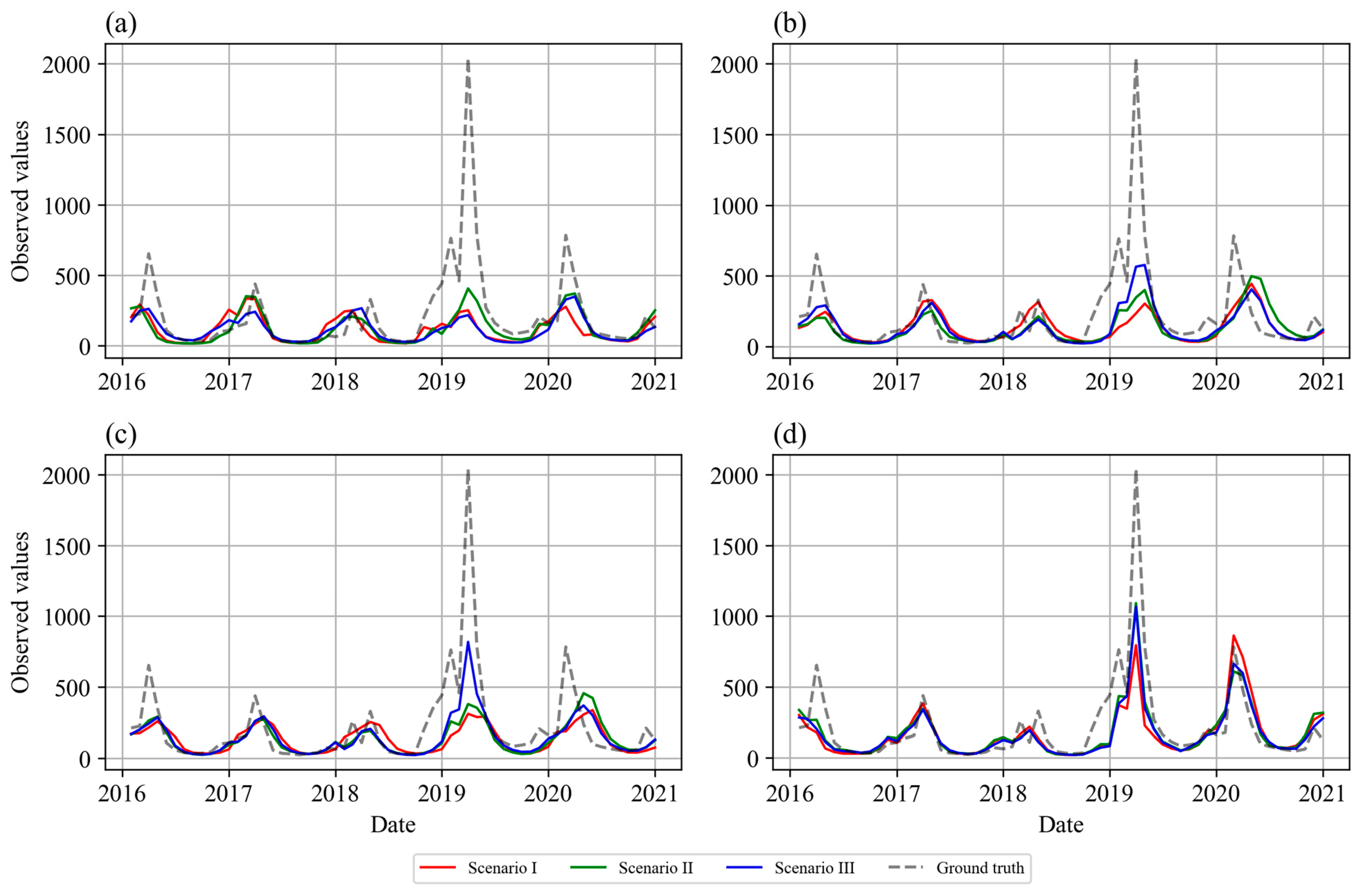
• SageFormer demonstrated its capability to predict the April 2019 flood event with the highest accuracy. The event, characterized by a 400-year return period, is inherently challenging to predict due to its rarity and intensity. While all other models underestimated the flood peak, SageFormer provided a near-accurate prediction, underscoring its effectiveness in modeling extreme hydrological events. This capability has significant implications for disaster risk reduction, particularly in data-scarce regions.
• In Scenario III, where cascading dimensionality reduction (DR) was applied, the curse of dimensionality was effectively mitigated, leading to improved prediction accuracy for attention-based models. SageFormer demonstrated its robustness in handling further dimensionality reduction, maintaining high accuracy (MAE: 0.481, MSE: 0.387) with only a minor decline in R² (0.661) compared to Scenario II. Informer also showed noticeable improvement in Scenario III, with MAE reducing from 0.591 to 0.523 and R² increasing from 0.470 to 0.573, underscoring the particular benefits of cascading DR for attention-based architectures.
• The improvement from Scenario I to Scenario II was the most pronounced for SageFormer, with a 10.6% reduction in MAE (0.539 to 0.482) and a 22.9% reduction in MSE (0.467 to 0.360).
• The Informer and Transformer models demonstrated moderate improvements, with Informer performing slightly better than Transformer in terms of R² (0.573 vs. 0.450) and Pearson correlation (0.782 vs. 0.730) in Scenario III. SageFormer outperformed Informer and Transformer significantly in all scenarios, particularly in Scenario III, where SageFormer achieved 8% lower MAE and 21% lower MSE compared to Informer.
• Vanilla LSTM showed the poorest-performing model across all scenarios, with limited capacity to model long-term dependencies and complex spatiotemporal relationships. While DR improved its performance from Scenario I (MAE: 0.776) to Scenario II (MAE: 0.685), cascading DR in Scenario III led to a slight degradation in R² (0.355) due to its inability to effectively handle further feature reduction.

Future studies should transform the deterministic forecasting framework into a probabilistic counterpart with improved performance and effectiveness to better inform decision-making and proactive flood management strategies. Additionally, employing transfer learning offers a promising direction, particularly for case studies with insufficient data or a lack of sufficiently large records for model training. This approach, similar to hydrological model calibration, leverages pre-trained models to enhance predictive capabilities and improve generalization in data-scarce environments.

References

1. Xu, X.; Xie, F.; Zhou, X. Research on Spatial and Temporal Characteristics of Drought Based on GIS Using Remote Sensing Big Data. Cluster Comput. 2016, 19, 757–767. [Google Scholar] [CrossRef]
2. Pham, T.M.; Dinh, H.T.; Pham, T.A.; Nguyen, T.S.; Duong, N.T. Modeling of Water Scarcity for Spatial Analysis Using Water Poverty Index and Fuzzy-MCDM Technique. Model. Earth Syst. Environ. 2024, 10, 2079–2097. [Google Scholar] [CrossRef]
3. Dolan, F.; Lamontagne, J.; Link, R.; Hejazi, M.; Reed, P.; Edmonds, J. Evaluating the Economic Impact of Water Scarcity in a Changing World. Nat. Commun. 2021, 12, 1915. [Google Scholar] [CrossRef] [PubMed]
4. Hussain, Z.; Wang, Z.; Yang, H.; Arfan, M.; Wang, W.; Faisal, M.; Azam, M.I.; Usman, M. Evolution and Trends of Water Scarcity Indicators: Unveiling Gaps, Challenges, and Collaborative Opportunities. Water Conserv. Sci. Eng. 2024, 9, 8. [Google Scholar] [CrossRef]
5. Fasihi, S.; Lim, W.Z.; Wu, W.; Proverbs, D. Systematic Review of Flood and Drought Literature Based on Science Mapping and Content Analysis. Water 2021, 13, 2788. [Google Scholar] [CrossRef]
6. Trong, N.G.; Quang, P.N.; Van Cuong, N.; Le, H.A.; Nguyen, H.L.; Tien Bui, D. Spatial Prediction of Fluvial Flood in High-Frequency Tropical Cyclone Area Using TensorFlow 1D-Convolution Neural Networks and Geospatial Data. Remote Sens. 2023, 15, 5429. [Google Scholar] [CrossRef]
7. El Garnaoui, M.; Boudhar, A.; Nifa, K.; El Jabiri, Y.; Karaoui, I.; El Aloui, A.; Midaoui, A.; Karroum, M.; Mosaid, H.; Chehbouni, A. Nested Cross-Validation for HBV Conceptual Rainfall–Runoff Model Spatial Stability Analysis in a Semi-Arid Context. Remote Sens. 2024, 16, 3756. [Google Scholar] [CrossRef]
8. Dommo, A.; Aloysius, N.; Lupo, A.; Hunt, S. Spatial and Temporal Analysis and Trends of Extreme Precipitation over the Mississippi River Basin, USA during 1988–2017. J. Hydrol. Reg. Stud. 2024, 56, 101954. [Google Scholar] [CrossRef]
9. UN Water. Climate Change and Water: UN-Water Policy Brief; UN Water: Geneva, Switzerland, 2019. [Google Scholar]
10. Sene, K. Hydrological Forecasting. Hydrometeorology 2024, 167–215. [Google Scholar] [CrossRef]
11. Sene, K. Hydrometeorology: Forecasting and Applications; Springer: Cham, Switzerland, 2015. [Google Scholar]
12. Zhou, F.; Chen, Y.; Liu, J. Application of a New Hybrid Deep Learning Model That Considers Temporal and Feature Dependencies in Rainfall–Runoff Simulation. Remote Sens. 2023, 15, 1395. [Google Scholar] [CrossRef]
13. Lo, W.C.; Wang, W.J.; Chen, H.Y.; Lee, J.W.; Vojinovic, Z. Feasibility Study Regarding the Use of a Conformer Model for Rainfall-Runoff Modeling. Water 2024, 16, 3125. [Google Scholar] [CrossRef]
14. Ghobadi, F.; Kang, D. Application of Machine Learning in Water Resources Management: A Systematic Literature Review. Water 2023, 15, 620. [Google Scholar] [CrossRef]
15. Ghobadi, F.; Kang, D. Improving Long-Term Streamflow Prediction in a Poorly Gauged Basin Using Geo-Spatiotemporal Mesoscale Data and Attention-Based Deep Learning: A Comparative Study. J. Hydrol. 2022, 615, 128608. [Google Scholar] [CrossRef]
16. Ghobadi, F.; Yaseen, Z.M.; Kang, D. Long-Term Streamflow Forecasting in Data-Scarce Regions: Insightful Investigation for Leveraging Satellite-Derived Data, Informer Architecture, and Concurrent Fine-Tuning Transfer Learning. J. Hydrol. 2024, 631, 130772. [Google Scholar] [CrossRef]
17. Sharafkhani, F.; Corns, S.; Holmes, R. Multi-Step Ahead Water Level Forecasting Using Deep Neural Networks. Water 2024, 16, 3153. [Google Scholar] [CrossRef]
18. Wang, Z.; Xu, N.; Bao, X.; Wu, J.; Cui, X. Spatio-Temporal Deep Learning Model for Accurate Streamflow Prediction with Multi-Source Data Fusion. Environ. Model. Softw. 2024, 178, 106091. [Google Scholar] [CrossRef]
19. Fayer, G.; Bolotari, N.; Miranda, F.; Ferreira, J.S.; da Silva, R.R.C.; Cândido, V.B.R.; Andrade, M.P.; Morais, M.; Ribeiro, C.B.M.; Capriles, P.V.Z.; et al. A Temporal Fusion Transformer Deep Learning Model for Long-Term Streamflow Forecasting: A Case Study in the Funil Reservoir, Southeast Brazil. Knowl. Based Eng. Sci. 2023, 4, 73–88. [Google Scholar]
20. Xu, Y.; Lin, K.; Hu, C.; Wang, S.; Wu, Q.; Zhang, L.; Ran, G. Deep Transfer Learning Based on Transformer for Flood Forecasting in Data-Sparse Basins. J. Hydrol. 2023, 625, 129956. [Google Scholar] [CrossRef]
21. Dtissibe, F.Y.; Ari, A.A.A.; Abboubakar, H.; Njoya, A.N.; Mohamadou, A.; Thiare, O. A Comparative Study of Machine Learning and Deep Learning Methods for Flood Forecasting in the Far-North Region, Cameroon. Sci. Afr. 2024, 23. [Google Scholar] [CrossRef]
22. Malik, H.; Feng, J.; Shao, P.; Abduljabbar, Z.A. Improving Flood Forecasting Using Time-Distributed CNN-LSTM Model: A Time-Distributed Spatiotemporal Method. Earth Sci. Inform. 2024, 17, 3455–3474. [Google Scholar] [CrossRef]
23. Bennett, A.; Tran, H.; De la Fuente, L.; Triplett, A.; Ma, Y.; Melchior, P.; Maxwell, R.M.; Condon, L.E. Spatio-Temporal Machine Learning for Regional to Continental Scale Terrestrial Hydrology. J. Adv. Model. Earth Syst. 2024, 16, e2023MS004095. [Google Scholar] [CrossRef]
24. Kow, P.Y.; Liou, J.Y.; Sun, W.; Chang, L.C.; Chang, F.J. Watershed Groundwater Level Multi-step Ahead Forecasts by Fusing Convolutional-Based Autoencoder and LSTM Models. J. Environ. Manag. 2024, 351, 119789. [Google Scholar] [CrossRef] [PubMed]
25. Li, W.; Liu, C.; Xu, Y.; Niu, C.; Li, R.; Li, M.; Hu, C.; Tian, L. An Interpretable Hybrid Deep Learning Model for Flood Forecasting Based on Transformer and LSTM. J. Hydrol. Reg. Stud. 2024, 54, 101873. [Google Scholar] [CrossRef]
26. Perera, U.A.K.K.; Coralage, D.T.S.; Ekanayake, I.U.; Alawatugoda, J.; Meddage, D.P.P. A New Frontier in Streamflow Modeling in Ungauged Basins with Sparse Data: A Modified Generative Adversarial Network with Explainable AI. Results Eng. 2024, 21, 101920. [Google Scholar] [CrossRef]
27. Bloemheuvel, S.; van den Hoogen, J.; Atzmueller, M. Graph Construction on Complex Spatiotemporal Data for Enhancing Graph Neural Network-Based Approaches. Int. J. Data Sci. Anal. 2024, 18, 157–174. [Google Scholar] [CrossRef]
28. Taccari, M.L.; Wang, H.; Nuttall, J.; Chen, X.; Jimack, P.K. Spatial-Temporal Graph Neural Networks for Groundwater Data. Sci. Rep. 2024, 14, 1–12. [Google Scholar] [CrossRef]
29. Zhang, Z.; Meng, L.; Gu, Y. SageFormer: Series-Aware Framework for Long-Term Multivariate Time-Series Forecasting. IEEE Internet Things J. 2024, 11. [Google Scholar] [CrossRef]
30. Vaswani, A.; Shazeer, N.; Parmar, N.; Uszkoreit, J.; Jones, L.; Gomez, A.N.; Kaiser, Ł.; Polosukhin, I.; Kaiser, L.; Polosukhin, I. Attention Is All You Need. Adv. Neural Inf. Process. Syst. 2017. [Google Scholar]
31. Ghobadi, F.; Saman, A.; Charmchi, T.; Kang, D. Feature Extraction from Satellite-Derived Hydroclimate Data: Assessing Impacts on Various Neural Networks for Multi-Step Ahead Streamflow Prediction. Sustainability 2023, 15, 15761. [Google Scholar] [CrossRef]
32. Zhou, H.; Zhang, S.S.; Peng, J.; Zhang, S.S.; Li, J.; Xiong, H.; Zhang, W. Informer: Beyond Efficient Transformer for Long Sequence Time-Series Forecasting. Proc. AAAI Conf. Artif. Intell. 2021, 35, 11106–11115. [Google Scholar] [CrossRef]
33. Freeman, E.; Woodruff, S.D.; Worley, S.J.; Lubker, S.J.; Kent, E.C.; Angel, W.E.; Berry, D.I.; Brohan, P.; Eastman, R.; Gates, L.; et al. ICOADS Release 3.0: A Major Update to the Historical Marine Climate Record. Int. J. Climatol. 2017, 37, 2211–2232. [Google Scholar] [CrossRef]
34. Schneider, U.; Finger, P.; Meyer-Christoffer, A.; Rustemeier, E.; Ziese, M.; Becker, A. Evaluating the Hydrological Cycle over Land Using the Newly-Corrected Precipitation Climatology from the Global Precipitation Climatology Centre (GPCC). Atmosphere 2017, 8, 52. [Google Scholar] [CrossRef]
35. Bennett, N.D.; Croke, B.F.W.; Guariso, G.; Guillaume, J.H.A.; Hamilton, S.H.; Jakeman, A.J.; Marsili-Libelli, S.; Newham, L.T.H.; Norton, J.P.; Perrin, C.; et al. Characterising Performance of Environmental Models. Environ. Model. Softw. 2013, 40, 1–20. [Google Scholar] [CrossRef]
36. Moriasi, D.N.; Gitau, M.W.; Pai, N.; Daggupati, P. Hydrologic and Water Quality Models: Performance Measures and Evaluation Criteria. Trans. ASABE 2015, 58, 1763–1785. [Google Scholar] [CrossRef]
37. Kingston, D.G.; McGregor, G.R.; Hannah, D.M.; Lawler, D.M. River Flow Teleconnections across the Northern North Atlantic Region. Geophys. Res. Lett. 2006, 33. [Google Scholar] [CrossRef]
38. Abbasi, M.; Farokhnia, A.; Bahreinimotlagh, M.; Roozbahani, R. A Hybrid of Random Forest and Deep Auto-Encoder with Support Vector Regression Methods for Accuracy Improvement and Uncertainty Reduction of Long-Term Streamflow Prediction. J. Hydrol. 2021, 597, 125717. [Google Scholar] [CrossRef]
Figure 1. Schematic representation of (a) the proposed framework, delineated in five key steps, and (b) the modeling flowchart employed in this study.
Remotesensing 17 00365 g001aRemotesensing 17 00365 g001b
Figure 2. Location of the Karkheh River basin and Karkheh Dam within the study domain.
Remotesensing 17 00365 g002
Figure 3. The scaled values of the three gridded input features over 12 months for (a) SST, (b) MSLP, and (c) Precip.
Remotesensing 17 00365 g003
Figure 4. Geo-spatiotemporal correlation between (a) SST, (b) MSLP, and (c) Precip data and streamflow for lags 1 to 12 in the selected domain.
Remotesensing 17 00365 g004
Figure 5. Cross-correlation between streamflow and (a) SST, (b) MSLP, (c) Precip, and (d) streamflow autocorrelation.
Remotesensing 17 00365 g005
Figure 6. Selected grids with a predefined filter corresponding to a high correlation (0.7) between (a) SST, (b) MSLP, and (c) Precip and field-measured streamflow for lags 1 to 12 in the selected domain.
Remotesensing 17 00365 g006
Figure 7. Selected (a) SST, (b) MSLP, and (c) Precip grids as input into the SageFormer for lags 1 to 12 in the selected domain.
Remotesensing 17 00365 g007
Figure 8. Scatter plots comparing the predictive performances of the (a) Vanilla LSTM, (b) Transformer, (c) Informer, and (d) SageFormer models under three scenarios.
Remotesensing 17 00365 g008
Figure 9. Forecasting performance of (a) Vanilla LSTM, (b) Transformer, (c) Informer, and (d) SageFormer over five successive years (test set) under three scenarios (standardized values).
Remotesensing 17 00365 g009
Figure 10. Forecasting performance of (a) Vanilla LSTM, (b) Transformer, (c) Informer, and (d) SageFormer over five successive years (test set) under three scenarios (actual values).
Remotesensing 17 00365 g010
Figure 11. Residual errors of all models under (a) Scenario I, (b) Scenario II, and (c) Scenario III. Two flood events are highlighted in gray.
Remotesensing 17 00365 g011