Spatiotemporal Variations in Vegetation Phenology in the Qinling Mountains and Their Responses to Climate Variability

Highlights

What are the main findings?

• Vegetation phenology baselines (mean SOS) are spatially constrained by altitude and vegetation type, exhibiting highly significant heterogeneity ($p < 0.001$).
• Conversely, interannual phenology trends (slopes) are statistically uniform across all vegetation types ($p = 0.685$), demonstrating a “temporal convergence” driven by a unified regional climate signal (spring temperature).

What are the implications of the main findings?

• The phenological response is asymmetric: a highly sensitive spring (SOS) is combined with a climatically insensitive autumn (EOS), revealing an “ecological buffering mechanism” that stabilizes the overall growing season length against interannual climate variability.
• The systematic ANCOVA framework successfully separates spatial heterogeneity from temporal trends, challenging the common assumption of “fragmented” phenological responses and providing a rigorous statistical approach to detect unified climate signals in complex mountain ecosystems.

Abstract

Understanding vegetation phenology responses to climate change is essential for predicting ecosystem dynamics, especially in mountainous transition zones, such as the Qinling Mountains, where climatic and ecological gradients are pronounced. To quantify these complex interactions, we combined high spatiotemporal resolution remote sensing data (30 m, 8-day) with CMFD climate datasets from 2010 to 2020. We leveraged a rigorous analysis of covariance (ANCOVA) framework to simultaneously test the spatial heterogeneity of phenological baselines and the temporal convergence of trends across vegetation types. Results revealed that the spatial pattern of the start of the growing season (SOS) exhibited highly significant heterogeneity (p < 0.001), primarily governed by vegetation composition and altitudinal gradients—a phenomenon we define as a spatial baseline constraint effect. In contrast, the interannual SOS trends (slopes) showed no significant differences among vegetation types (p = 0.685), indicating a temporal convergence effect. This regional synchrony, characterized by a consistent shift toward earlier SOS of approximately −0.8 to −0.9 days yr⁻¹ at low and mid-elevations, was largely driven by rising spring temperatures (R² ≈ 0.20). Crucially, the end of the growing season (EOS) displayed weak climatic sensitivity, revealing an asymmetric phenological response to temperature changes. Our findings demonstrate that vegetation phenology in the Qinling Mountains is jointly controlled by spatial baseline constraint and temporal trend convergence. This dual-mechanism framework provides new insights into the highly structured stability and resilience of mountainous ecosystems under regional warming.

1. Introduction

Vegetation phenology, the seasonal timing of plant growth and senescence, serves as a sensitive indicator of ecosystem responses to climate change [1,2]. Over recent decades, widespread phenological shifts—particularly earlier spring onset and delayed autumn senescence—have been documented across the globe [3], reflecting the profound ecological imprint of global warming [4]. These shifts not only influence regional carbon and water cycles [5] but also alter ecosystem productivity and species interactions [6,7].

However, in mountainous ecosystems, such as the Qinling Mountains of central China [8], phenological responses to climate change exhibit far greater complexity than in lowland regions [9,10]. The Qinling range forms a prominent biogeographic boundary between northern and southern China [11,12], encompassing steep climatic and ecological gradients within relatively short distances [13]. This makes it an ideal yet challenging setting for disentangling how topography, vegetation composition, and microclimate jointly shape phenological dynamics [11].

Spatial heterogeneity—arising from elevation, vegetation type, and exposure—remains a major challenge in understanding mountain phenology [14]. Previous studies have frequently reported spatially fragmented or localized phenological trends in mountainous regions [15], often relying on coarser resolution data or simpler regression models [16]. Yet, the underlying causes of such heterogeneity remain debated: are these patterns driven by genuine ecological processes—such as differential temperature sensitivities [17]—or do they partially arise from methodological artifacts, such as inadequate statistical tests [18]? Disentangling the source of heterogeneity in the trend (slope) is crucial for accurately assessing how ecosystems respond to ongoing climate change [19].

To accurately capture the spatial heterogeneity of vegetation phenology in complex mountainous terrain, the spatial resolution of remote sensing data is critical [20]. Coarse-resolution products often mask the intricate variations caused by fragmented topography and diverse vegetation communities [21]. In this study, we utilized a 30 m fused NDVI time-series product, which offers a significant advantage over traditional coarse-resolution datasets [22]. This high-resolution product is particularly valuable for mountainous ecosystems like the Qinling Mountains, as it allows for the retrieval of phenology metrics at a scale appropriate for resolving the fine-scale interactions between topography, vegetation occurrence, and microclimate. By integrating this 30 m product with topographic and climatic data, we can more effectively assess the spatial heterogeneity of phenological responses that might otherwise be homogenized in coarser pixels [23].

Vegetation phenology is typically characterized by key metrics such as the Start of Season (SOS), End of Season (EOS), and Growing Season Length (GSL), each playing a distinct role in ecosystem dynamics. SOS is a critical indicator of spring onset and is strongly sensitive to pre-season temperature and precipitation, directly influencing ecosystem productivity and carbon uptake [24,25]. EOS marks the cessation of growth and is often regulated by a complex interplay of temperature, water availability, and photoperiod [26]. Together, SOS and EOS determine the GSL, which represents the total duration of photosynthetic activity. Understanding the spatiotemporal shifts in these metrics is essential for unraveling how mountain ecosystems respond to climate variability and for predicting future changes in regional carbon and water cycles [27].

Accordingly, this study aims to provide a comprehensive examination of vegetation phenology in the Qinling Mountains using high-resolution remote sensing and climate datasets. Specifically, we seek to:

(1)

Statistically test whether the baseline phenological state (i.e., mean start of season, SOS) exhibits spatial heterogeneity governed by elevation and vegetation type;

(2)

Determine whether interannual phenological trends (slopes) differ significantly across vegetation units or instead converge toward a common climatic driver;

(3)

Identify the dominant climatic factors—particularly the relative roles of temperature and precipitation—that regulate these phenological changes.

By addressing these objectives, we propose a dual-mechanism framework of “spatial baseline constraint” and “temporal trend convergence”, aiming to reveal how structural heterogeneity and climatic synchronization jointly shape phenological dynamics in mountainous ecosystems.

2. Materials and Methods

2.1. Study Area

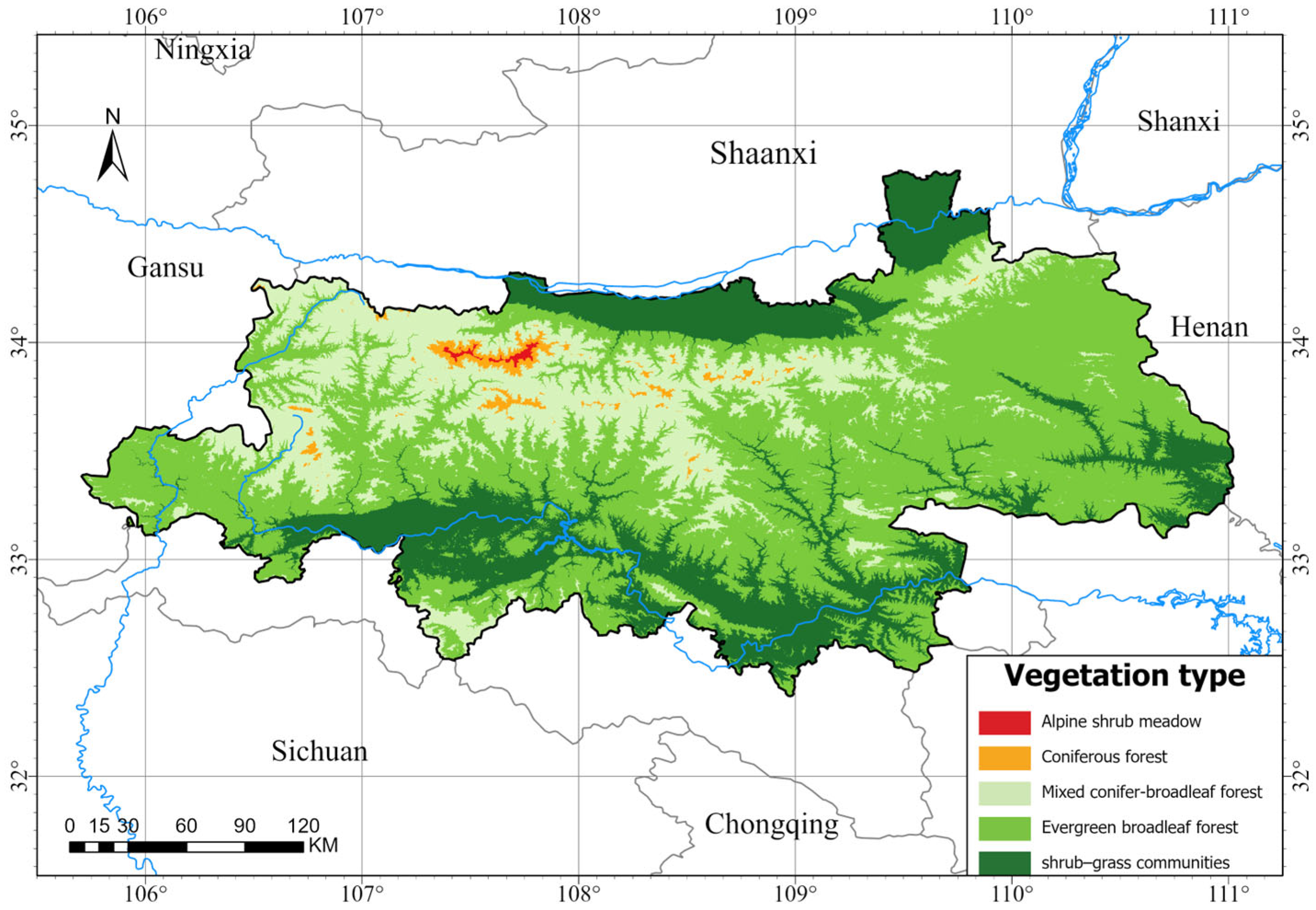
The study area covers the Qinling Mountains, an east–west–oriented mountain range located in central China [19]. This region represents an important climatic and biogeographical boundary between northern and southern China. The selected study extent is primarily situated within Shaanxi Province and encompasses a complete elevational gradient from low-mountain shrub–grass communities to subalpine coniferous forests and alpine meadows (Figure 1 and Figure 2). Pronounced climatic contrasts between the northern and southern slopes shape distinct vertical ecological zonation, providing an ideal natural laboratory for investigating vegetation phenological responses to climate variability

Due to their east–west orientation and substantial topographic relief, the Qinling Mountains serve as a crucial climatic divide, effectively constraining atmospheric circulation patterns. The mountains block the northward extent of the East Asian summer monsoon and shield the south from cold continental air masses. This topographic forcing results in a pronounced climatic and ecological transition: the northern slopes are dominated by a warm-temperate semi-humid to semi-arid climate, while the southern slopes foster a humid subtropical climate, supporting diverse vegetation communities.

Vegetation distribution follows a clear vertical zonation pattern (Figure 2). Below approximately 700 m, the landscape is dominated by shrub–grass communities typical of low hills. Between 700 m and 1500 m, evergreen broadleaf forests prevail, forming the lower montane vegetation belt. Mixed conifer–broadleaf forests dominate the mid-montane zone (1500–2400 m), followed by pure coniferous forests between 2400 m and 3100 m. Above 3100 m, alpine shrubs and meadows extend to the highest peaks around 3760 m.

This pronounced topographic and climatic heterogeneity provides a natural setting for investigating how vegetation phenology responds to elevation and climate variation [28].

2.2. Data Sources and Preprocessing

2.2.1. NDVI Data

We used the 30 m fused NDVI time-series dataset generated by external research teams based on the Integrated Environmental Variable Spatiotemporal Fusion Model (InENVI) [29,30]. This product integrates multi-source surface reflectance observations and features high spatial consistency and temporal continuity [31]. The selected time span is 2010–2020, with an 8-day temporal resolution. The dataset is provided in HDF format (WGS84, EPSG:4326). This period was chosen to focus on interannual phenological variations in response to the recent decade of climate change.

2.2.2. Meteorological Data

Air temperature and precipitation data were obtained from the China Meteorological Forcing Dataset (CMFD) [32,33], with a spatial resolution of approximately 0.01° (~1 km). To match the 8-day NDVI composite interval, the daily CMFD variables were aggregated to 8-day means (temperature) or 8-day totals (precipitation), producing climate time series fully aligned with the NDVI sequence.

2.2.3. Topography and Vegetation Data

Topographic information was derived from the 30 m Global Digital Elevation Model (GDEM) [34] and used for the delineation of elevation zones and interpretation of vegetation belts. Vegetation types were categorized into five representative vegetation zones following the vertical zonation characteristics of the Qinling Mountains. All datasets were clipped to the unified study boundary and co-registered using a geometric lookup table (GLT) or equivalent pixel-level alignment method.

2.3. Extraction of Remote Sensing Phenology and Definition of Seasonal Variables

2.3.1. NDVI Preprocessing and Smoothing

For each pixel, the NDVI time series was preprocessed, including missing-value masking and radiometric corrections. We applied the Whittaker smoother (parameter settings following high-resolution phenology extraction guidelines) to suppress residual noise caused by cloud contamination and atmospheric disturbances while preserving seasonal transition features essential for phenology detection [35].

2.3.2. Phenological Metrics Extraction

After smoothing, phenological parameters were extracted annually using the relative-threshold method [36]. The phenological threshold ${\mathrm{N}\mathrm{D}\mathrm{V}\mathrm{I}}_{\mathrm{t}\mathrm{h}}$ was defined as:

$${\mathrm{N}\mathrm{D}\mathrm{V}\mathrm{I}}_{\mathrm{t}\mathrm{h}}={\mathrm{N}\mathrm{D}\mathrm{V}\mathrm{I}}_{\mathrm{m}\mathrm{i}\mathrm{n}}+0.5\times ({\mathrm{N}\mathrm{D}\mathrm{V}\mathrm{I}}_{\mathrm{m}\mathrm{a}\mathrm{x}}-{\mathrm{N}\mathrm{D}\mathrm{V}\mathrm{I}}_{\mathrm{m}\mathrm{i}\mathrm{n}})$$

(1)

Pixels with an annual NDVI amplitude below 0.02 were discarded as invalid for phenology retrieval.

2.3.3. Definition of Seasonal Climate Variables

Based on the 8-day climate series, seasonal variables were constructed for phenology–climate sensitivity analyses. Examples include spring mean temperature ($T_{\mathrm{s}\mathrm{p}\mathrm{r}\mathrm{i}\mathrm{n}\mathrm{g}}$), identified as the dominant thermal driver of SOS, and seasonal precipitation metrics ($P_{\mathrm{s}\mathrm{p}\mathrm{r}\mathrm{i}\mathrm{n}\mathrm{g}},P_{\mathrm{a}\mathrm{u}\mathrm{t}\mathrm{u}\mathrm{m}\mathrm{n}}$).

2.4. Statistical Analyses

2.4.1. Trend Analysis

Interannual trends of SOS were quantified for each vegetation type and elevation zone using ordinary least squares (OLS) regression [37]:

$$\mathrm{S}\mathrm{O}\mathrm{S}=b_0+b_1\times \mathrm{Y}\mathrm{e}\mathrm{a}\mathrm{r}+ϵ$$

(2)

where $b_1$ represents the trend slope. Diagnostic checks on residuals and model fit were performed, and extreme outliers were masked to ensure robustness.

2.4.2. Pixel-Scale Climate Sensitivity Analysis

Pixel-wise correlation (Pearson $r$ and Spearman rank correlation) and linear regression analyses were used to quantify the sensitivity of phenology to climate variables [38]:

$$\mathrm{P}\mathrm{h}\mathrm{e}\mathrm{n}\mathrm{o}=a+b\times \mathrm{C}\mathrm{l}\mathrm{i}\mathrm{m}\mathrm{a}\mathrm{t}\mathrm{e}+ϵ$$

(3)

where Pheno represents phenological metrics and Climate denotes seasonal climate variables. The slope $b$ indicates climate sensitivity (e.g., SOS shift per °C change), and the coefficient of determination $R^2$ describes the explanatory power. Statistical significance was evaluated at $\alpha =0.05$.

2.4.3. ANCOVA for Testing Differences Among Vegetation Types

To simultaneously examine baseline differences and interannual trends across vegetation types, an analysis of covariance (ANCOVA) model was applied [39,40]:

$$\mathrm{S}\mathrm{O}\mathrm{S}={\beta }_0+{\beta }_1{\mathrm{Y}\mathrm{e}\mathrm{a}\mathrm{r}}_{\mathrm{C}\mathrm{e}\mathrm{n}\mathrm{t}\mathrm{e}\mathrm{r}\mathrm{e}\mathrm{d}}+{\beta }_{2}C\left(\mathrm{V}\mathrm{e}\mathrm{g}\mathrm{e}\mathrm{t}\mathrm{a}\mathrm{t}\mathrm{i}\mathrm{o}\mathrm{n}\right)+{\beta }_3({\mathrm{Y}\mathrm{e}\mathrm{a}\mathrm{r}}_{\mathrm{C}\mathrm{e}\mathrm{n}\mathrm{t}\mathrm{e}\mathrm{r}\mathrm{e}\mathrm{d}}\times C(\mathrm{V}\mathrm{e}\mathrm{g}\mathrm{e}\mathrm{t}\mathrm{a}\mathrm{t}\mathrm{i}\mathrm{o}\mathrm{n}\left)\right)+ϵ$$

(4)

where ${\mathrm{Y}\mathrm{e}\mathrm{a}\mathrm{r}}_{\mathrm{C}\mathrm{e}\mathrm{n}\mathrm{t}\mathrm{e}\mathrm{r}\mathrm{e}\mathrm{d}}$ denotes the centered year.

Main effect $C\left(\mathrm{V}\mathrm{e}\mathrm{g}\mathrm{e}\mathrm{t}\mathrm{a}\mathrm{t}\mathrm{i}\mathrm{o}\mathrm{n}\right)$: tests baseline SOS differences among vegetation types.

Interaction term ${\mathrm{Y}\mathrm{e}\mathrm{a}\mathrm{r}}_{\mathrm{C}\mathrm{e}\mathrm{n}\mathrm{t}\mathrm{e}\mathrm{r}\mathrm{e}\mathrm{d}}\times C\left(\mathrm{V}\mathrm{e}\mathrm{g}\mathrm{e}\mathrm{t}\mathrm{a}\mathrm{t}\mathrm{i}\mathrm{o}\mathrm{n}\right)$: tests whether interannual SOS trends differ across vegetation types.

ANCOVA was conducted at two scales to ensure robustness: Pixel-level random sampling, summarizing parameter distributions by vegetation type. Aggregated zonal means, fitting the model to time series averaged within vegetation or elevation strata.

3. Results

3.1. Data Verification and Phenological Baseline

Before conducting a comprehensive analysis of vegetation phenological dynamics, we first evaluated the reliability of the phenological parameters extracted from the 30-m resolution InENVI dataset. The extracted growing season start time (SOS) ranged from day 73 to day 88, and the growing season end time (EOS) ranged from day 306 to day 323. These values are in perfect agreement with the typical ranges reported in previous studies based on MODIS, Landsat, and other multi-source remote sensing products (

Table 1. Comparison of growing season phenological metrics (SOS and EOS) in the Qinling Mountains derived from this study and previously published datasets. The table summarizes reported SOS and EOS ranges from MODIS- and Landsat-based studies using different vegetation indices, spatial–temporal resolutions, and extraction methods. The SOS and EOS values obtained from the fused InENVI NDVI dataset (73–88 DOY and 306–323 DOY, respectively) fall well within the ranges documented in previous studies, confirming the reliability and consistency of the fused product for fine-scale phenological analysis in complex mountain environments.

Region	VI	Data Source	Spatial	Temporal	Method	SOS	EOS
Qinling Mountains [41]	NDVI	MODIS	1 km	16 d	Savitzky–Golay	83–121 d	290–300 d
Qinling–Daba Mountains [42]	NDVI	MODIS	250 m	16 d	Linear regression analysis	80–134 d	275–315 d
Qinling-Niubeiliang	NDVI	MODIS	250 m	8 d	Threshold	115–140 d	260–300 d
Qinling Mountains [43]	EVI	MODIS	250 m	16 d	Savitzky–Golay	73–105 d	——
Qinling Mountains [19]	EVI	MODIS	500 m	8 d	HANTS	81–120 d	260–310 d
Qinling–Daba Mountains [11]	NDVI	MODIS	250 m	8 d	Max-ratio	70–130 d	270–310 d
Qinling Mountains [44]	NDVI	MODIS	500 m	8 d	Max-ratio HANTS	81~120 d	270~311 d
Qinling Mountains [45]	NDVI	MODIS	250 m	10 d	Dynamic Threshold Method	120~130 d	300~325 d

) [11,19,41,42,43,44,45], indicating a high degree of consistency with existing literature. This consistency demonstrates that the preprocessing pipeline and phenological extraction methods used in our study are robust and well-suited for characterizing vegetation phenology under the complex topographic conditions of the Qinling Mountains.

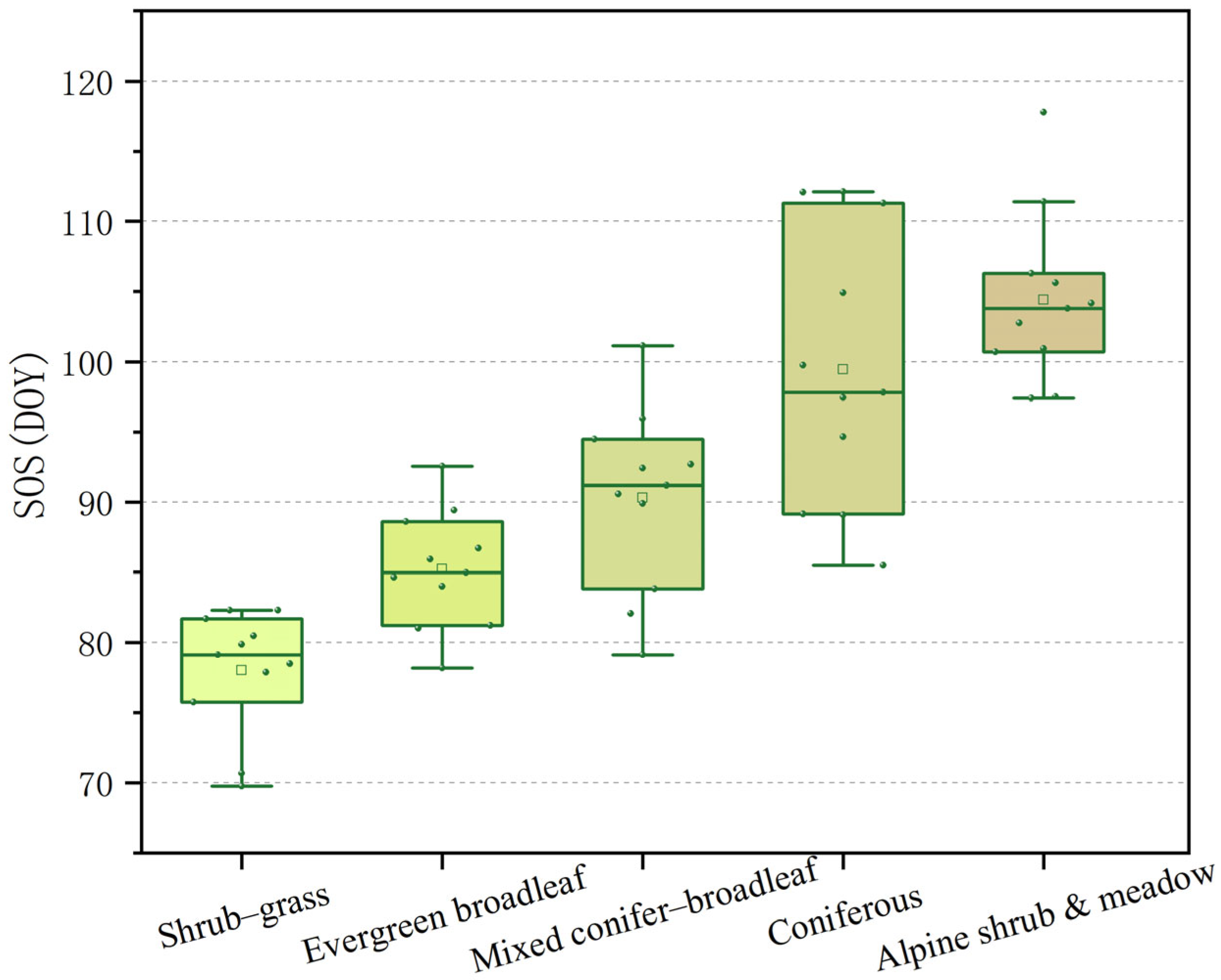
After determining the reliability of the data, we further investigated the spatial distribution of the phenological parameters. The results show significant spatial heterogeneity in the region, with the growing season start time differing particularly significantly between different vegetation functional types. As shown in (Figure 3), the spatial pattern of SOS is closely related to the altitudinal zonation of vegetation: shrub–grassland communities at low altitudes turn green earliest, followed by evergreen broad-leaved forests, mixed coniferous and broad-leaved forests, and finally high-altitude coniferous forests.

The influence of vegetation type was quantified using an analysis of covariance (ANCOVA) model (

Table 2. ANCOVA results for the effects of vegetation type and year on SOS. This table summarizes the ANCOVA results assessing the independent and interactive effects of vegetation type and centered year on the SOS. Vegetation type shows a highly significant main effect ($p<0.001$), indicating strong spatial differences in baseline SOS among vegetation zones. By contrast, the effect of interannual variation is not significant ($p=0.754$), and its interaction with vegetation type is also non-significant ($p=0.685$), demonstrating that SOS trends do not differ among vegetation types. These results support the conclusion that SOS is subject to strong spatial baseline heterogeneity but exhibits convergent temporal trends across vegetation categories.

Effect	F	p-Value	Interpretation
Vegetation	22.21	<0.001	Significant difference among vegetation types
Year	0.10	0.754	No temporal trend
Vegetation × Year	0.57	0.685	No differential temporal trend among vegetation types

), and the results showed that the main effect was extremely significant (F = 22.21, p = 3.56 × 10⁻¹⁰). Regression coefficients indicated that compared with high-altitude coniferous forests, the SOS of shrub–grassland and evergreen broad-leaved forests occurred 24.28 days and 17.10 days earlier, respectively (both p < 0.001). In summary, these results indicate that the spatial baseline of vegetation phenology in the Qinling Mountains is jointly shaped by vegetation type and altitude, constituting the basic structure of the phenological pattern in this region.

3.2. Significant Heterogeneity in Interannual Trends

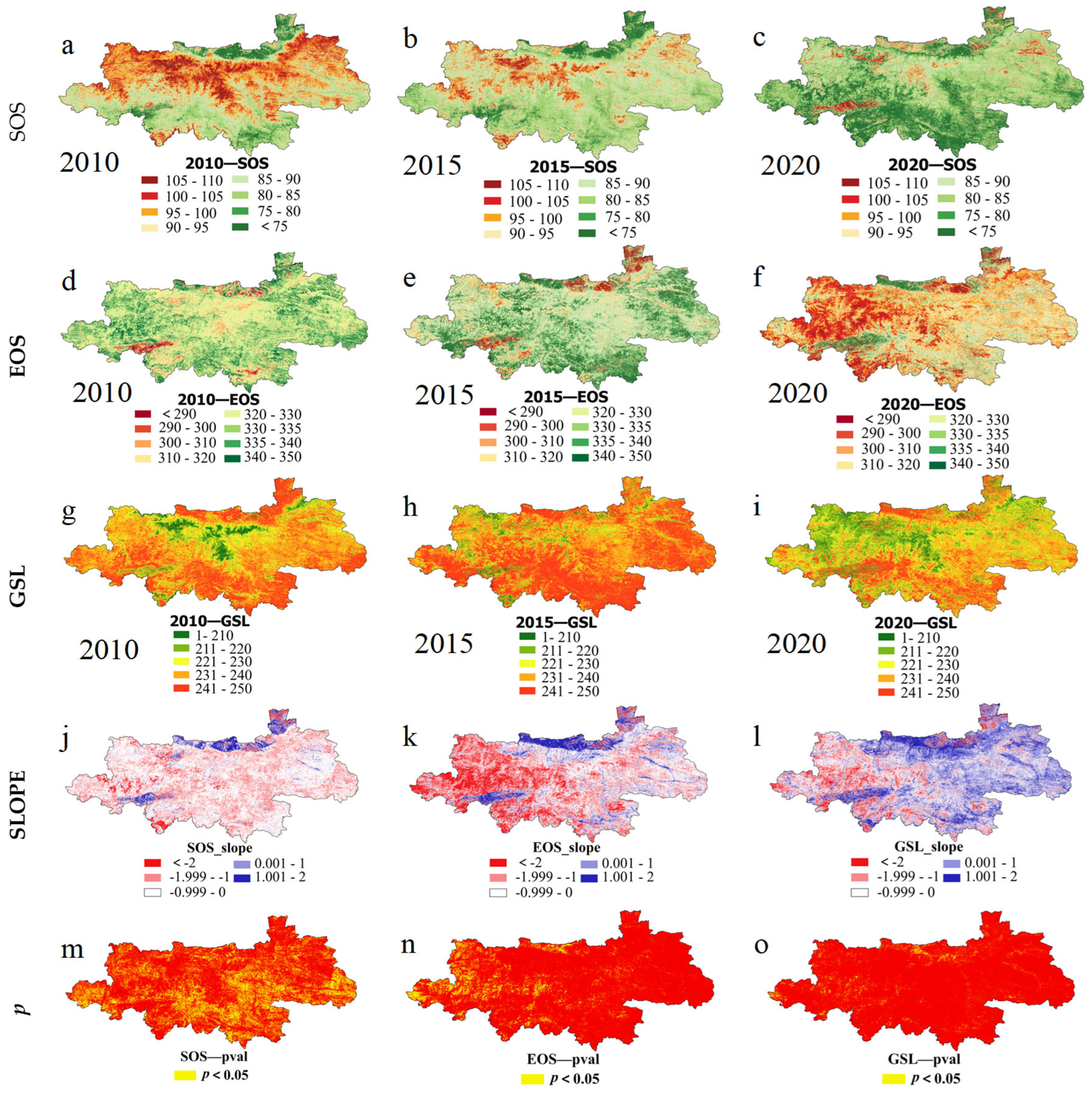
Based on the spatial baseline, we next examined the interannual variation in SOS from 2010 to 2020 (Figure 4). Pixel-by-pixel linear regression analysis revealed a significant overall trend of earlier onset, with an average rate of −0.71 days per year. Approximately 27% of pixels showed statistically significant earlier onset (p < 0.05), forming spatial clusters primarily concentrated within evergreen broad-leaved forests (Figure 5). During the study period, 2019 was the earliest year for SOS, with an average onset of only 73.01 days.

These pixel-scale results provide preliminary evidence of spatial heterogeneity in phenological trends, offering context for subsequent trend commonality testing using the ANCOVA framework.

Spatially, the areas with significantly earlier SOS were concentrated in mid-to-low altitude evergreen broad-leaved forests (Figure 5), indicating a faster phenological onset rate for this vegetation type. However, pixel-level regression is susceptible to various confounding factors, such as spatial autocorrelation, mixed pixels, or uneven vegetation type distribution. Therefore, whether this pattern represents a genuine ecological phenomenon or merely an analytical result requires further evaluation using a more rigorous statistical modeling framework.

3.3. Commonalities in Interannual Trends Among Different Vegetation Types

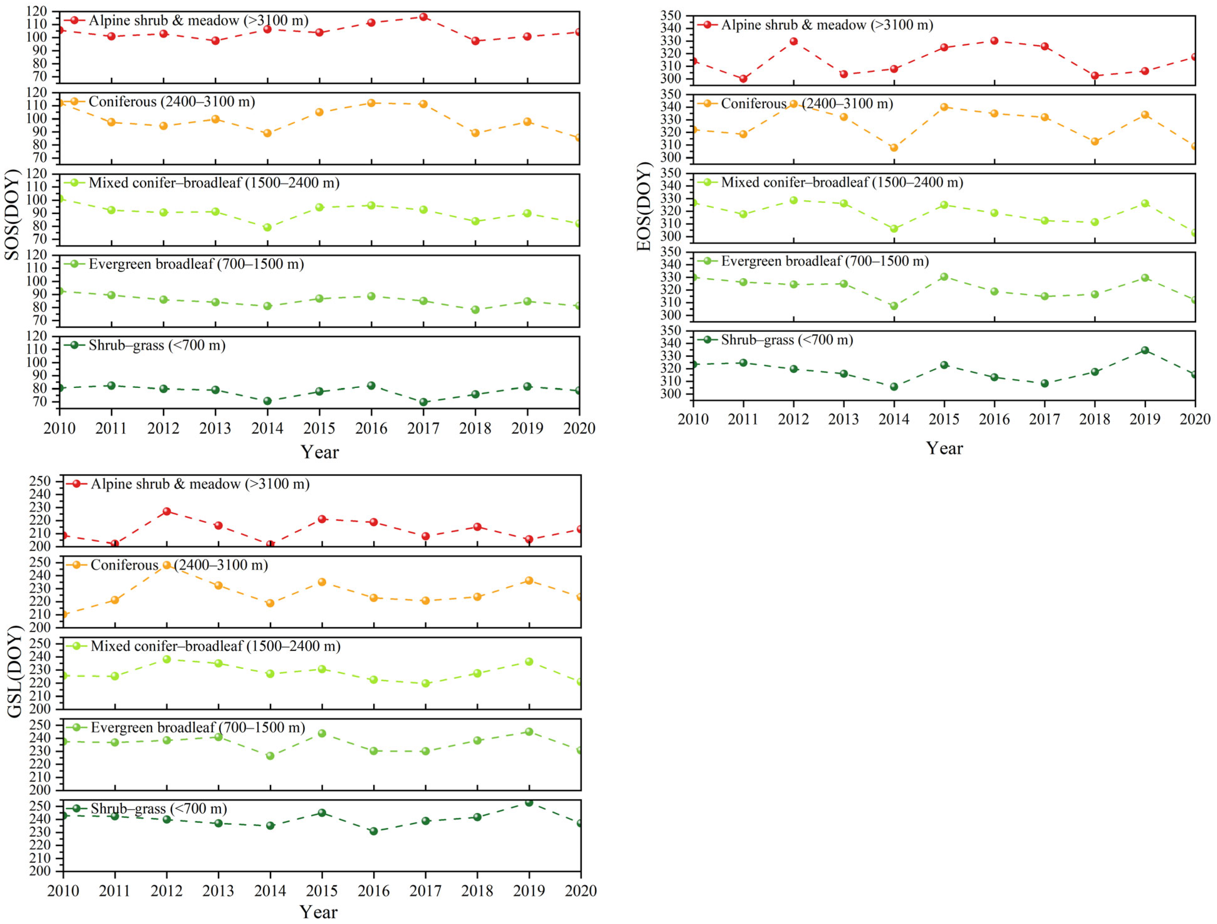
To formally assess whether there are significant differences in interannual phenological trends among different vegetation types, we constructed an analysis of covariance (ANCOVA) model including the interaction term between vegetation type and year (Table 2). This interaction term was not statistically significant (F = 0.57, p = 0.685), indicating that there were no significant differences in the SOS trends among different vegetation types. In other words, the perceived rate of shift toward earlier phenological timing in evergreen broad-leaved forests was not statistically significantly different from other vegetation types, meaning there was no obvious “sensitivity bias.” The main effect of the year variable also did not reach a significant level (p = 0.754), indicating that the phenological period in the Qinling Mountains as a whole did not show a consistent linear shift toward earlier or later dates between 2010 and 2020 (Figure 6).

In summary, although pixel-level results show a clustered distribution of pixels with significantly earlier phenological timing, the statistical model, after adjusting for vegetation type and other confounding factors, shows that the interannual rate of change is similar across all vegetation types. This reveals a significant “commonality” in phenological dynamics: interannual fluctuations across different vegetation types are largely synchronized, and differences in vegetation type are not the primary driving factor for phenological evolution.

3.4. Asymmetric Temperature Response

Given the lack of significant differences in the overall interannual trends of vegetation phenology, we further focus on the climate-driven mechanisms of interannual phenological fluctuations. Regression analysis results (Figure 7) show that spring temperature is the core driving factor influencing the earlier onset of SOS, with an explanatory power of 20% (R² ≈ 0.20), while the impact of precipitation on SOS is not statistically significant (p > 0.05). Notably, the response of vegetation phenology to temperature exhibits strong seasonal asymmetry: SOS is highly sensitive to spring warming (p < 0.001), while EOS shows no significant response to temperature changes or annual-scale changes (both p > 0.05).

This asymmetric temperature response directly results in: although SOS exhibits significant interannual fluctuations, the growing season length (GSL) does not show a significant linear trend due to the relative stability of EOS. In other words, the interannual fluctuations in vegetation phenology in the Qinling Mountains are mainly driven by the interannual variation in spring temperature, while autumn phenology shows a slight tendency to occur earlier during the study period. The synergistic effect of the two makes the total length of the growing season relatively stable.

4. Discussion

Our primary finding is that the phenological baseline is strongly constrained by spatial factors. This aligns with ecological expectations: altitudinal hydrothermal gradients dictate the phenological onset [46,47]. In the highly fragmented Qinling Mountains, the pronounced relief creates steep climatic gradients over short distances. The consistent segregation of mean SOS along these gradients confirms the validity of our vegetation zonation, but more crucially, establishes the statistical basis for separating spatial baselines from temporal trends in the ANCOVA framework [25]. The utilization of the 30 m high-resolution data further allows for a more detailed characterization of this constraint effect, revealing fine-scale variations that would be homogenized by the mixed-pixel effect inherent in coarser products [48]. This refined spatial perspective is essential for accurate modeling in complex mountain terrain.

While the spatial factors impose a strong constraint on the phenological baseline, the study’s core contribution is the re-evaluation of “trend heterogeneity” at the temporal scale. Previous studies in mountains, often relying on pixel-level analysis, frequently reported spatially fragmented or localized trends [49,50]. Indeed, our pixel-level analysis initially showed a large percentage of non-significant trends (only 27% significant), consistent with these conventional reports. However, the more rigorous ANCOVA model provided the definitive evidence: the interaction term between time and vegetation type was non-significant. This statistically proves that the interannual trend slopes do not differ significantly among vegetation types. This “temporal convergence” refutes the hypothesis of strong trend heterogeneity in mountain responses [51], supporting instead the dominance of a “regional common driver” potent enough to synchronize responses and override local micro-variations at the interannual scale. This finding underscores the power of systematic statistical analysis in revealing unified regional signals that are obscured by localized noise in simpler models [1].

This temporal synchronization, driven by the convergence of interannual trends, allows us to effectively identify the common driver as spring temperature [52], which is explored further in this section. The phenological response displays a pronounced asymmetry: SOS was highly sensitive to temperature [53], whereas EOS remained relatively stable. This result is consistent with recent global studies that distinguish the strong temperature control on spring onset from the complex, multi-factor control on autumn senescence [54]. The stability of EOS likely stems from co-limiting non-thermal factors, such as photoperiod, autumn water stress, or early frost. This combination of a “sensitive SOS” and “stable EOS” reveals a crucial ecological buffering mechanism [55], allowing the GSL to remain stable despite high interannual variability in spring, which is vital for maintaining ecosystem carbon sequestration capacity and water use efficiency in this transitional mountain zone.

Finally, we acknowledge several limitations in our current analysis and discuss the future outlook. First, the 10-year period is suited for analyzing “interannual variability” rather than “long-term trends”. Second, while spring temperature was the dominant driver, it only explained 20% of SOS variance, suggesting the remaining variance is driven by unmodeled factors [56]. These remaining factors should be the focus of future studies utilizing advanced machine learning techniques to better predict local phenological shifts. Finally, direct ground validation remains an urgent challenge in such complex terrain [57].

Overall, the dual-mechanism framework proposed in this study offers a new statistical perspective for disentangling spatial patterns and detecting unified climate signals in environmentally heterogeneous mountain landscapes [58]. It further highlights the crucial role of asymmetric phenological responses in sustaining ecosystem stability under climate variability, providing valuable implications for mountain vegetation monitoring and climate impact assessments.

5. Conclusions

Using high-resolution remote sensing data and a rigorous ANCOVA framework, this study systematically disentangled the phenological dynamics of the Qinling Mountains. The results demonstrate that regional vegetation phenology is not characterized by fragmented or highly heterogeneous trends; rather, it is jointly shaped by two mechanisms: spatial baseline constraint and temporal trend convergence.

Our analysis first shows that multi-year mean SOS exhibits pronounced spatial heterogeneity ($p<0.001$), tightly constrained by altitudinal gradients in hydrothermal conditions and vegetation zonation. More importantly, the interannual SOS trends do not differ significantly among vegetation types ($p=0.685$). This challenges the prevailing assumption of strong trend heterogeneity in mountain environments and indicates that all vegetation types are responding coherently to a regional-scale common driver.

This common driver was identified as spring temperature ($R^2\approx 0.20$). The phenological response displays a pronounced asymmetry: SOS is highly sensitive to spring warming, whereas EOS remains comparatively stable. Such an asymmetric SOS–EOS pattern suggests an ecological buffering mechanism that helps maintain a relatively stable growing-season length despite interannual climate fluctuations.

References

1. Piao, S.; Liu, Q.; Chen, A.; Janssens, I.A.; Fu, Y.; Dai, J.; Liu, L.; Lian, X.; Shen, M.; Zhu, X. Plant Phenology and Global Climate Change: Current Progresses and Challenges. Glob. Change Biol. 2019, 25, 1922–1940. [Google Scholar] [CrossRef] [PubMed]
2. Fang, J.; Li, X.; Xiao, J.; Yan, X.; Li, B.; Liu, F. Vegetation Photosynthetic Phenology Dataset in Northern Terrestrial Ecosystems. Sci. Data 2023, 10, 300. [Google Scholar] [CrossRef] [PubMed]
3. Nie, Y.; Wu, Z.; Chen, S.; Xu, Y.; Gong, Y.; Wang, H.; Xiao, Y.; Liu, Z.; Fu, Y.H. Divergent Impacts of Precipitation Regimes on Autumn Phenology in the Northern Hemisphere Mid- to High-Latitudes. Geophys. Res. Lett. 2025, 52, e2025GL117589. [Google Scholar] [CrossRef]
4. Dang, C.; Shao, Z.; Huang, X.; Zhuang, Q.; Cheng, G.; Qian, J. Climate Warming-Induced Phenology Changes Dominate Vegetation Productivity in Northern Hemisphere Ecosystems. Ecol. Indic. 2023, 151, 110326. [Google Scholar] [CrossRef]
5. Yin, H.; Ma, X.; Liao, X.; Ye, H.; Yu, W.; Li, Y.; Wei, J.; Yuan, J.; Liu, Q. Linking Vegetation Phenology to Net Ecosystem Productivity: Climate Change Impacts in the Northern Hemisphere Using Satellite Data. Remote Sens. 2024, 16, 4101. [Google Scholar] [CrossRef]
6. Wang, N.; Jiao, A.; Xu, Y.; Yang, Y.; Cong, N.; Yao, W. Divergent Responses of Vegetation Phenology and Productivity to Climate Change in Typical River Basins across Northern and Southern China. J. Plant Ecol. 2025, 18, rtaf080. [Google Scholar] [CrossRef]
7. Jia, P.; Zhang, R.; Schmid, B.; Wang, H.; He, J.; Liu, J.; Liu, S.; Jian, S.; Feng, Y. A Global Synthesis of How Plants Respond to Climate Warming From Traits to Fitness. Ecol. Lett. 2025, 28, e70114. [Google Scholar] [CrossRef]
8. Touhami, I.; Moutahir, H.; Assoul, D.; Bergaoui, K.; Aouinti, H.; Bellot, J.; Andreu, J.M. Multi-Year Monitoring Land Surface Phenology in Relation to Climatic Variables Using MODIS-NDVI Time-Series in Mediterranean Forest, Northeast Tunisia. Acta Oecologica 2022, 114, 103804. [Google Scholar] [CrossRef]
9. Xu, S.; Yu, Z.; Lettenmaier, D.P.; McVicar, T.R.; Ji, X. Elevation-Dependent Response of Vegetation Dynamics to Climate Change in a Cold Mountainous Region. Environ. Res. Lett. 2020, 15, 094005. [Google Scholar] [CrossRef]
10. Cui, X.; Xu, G.; He, X.; Luo, D. Influences of Seasonal Soil Moisture and Temperature on Vegetation Phenology in the Qilian Mountains. Remote Sens. 2022, 14, 3645. [Google Scholar] [CrossRef]
11. Deng, C.H.; Bai, H.Y.; Ma, X.P.; Huang, X.Y.; Zhao, T. Variation characteristics and its north-south differences of the vegetation phenology by remote sensing monitoring in the Qinling Mountains during 2000–2017. Acta Ecol. Sin. 2021, 41, 1068–1080. [Google Scholar] [CrossRef]
12. Chen, X.; Zhang, Y. Impacts of Climate, Phenology, Elevation and Their Interactions on the Net Primary Productivity of Vegetation in Yunnan, China under Global Warming. Ecol. Indic. 2023, 154, 110533. [Google Scholar] [CrossRef]
13. Xue, Y.; Bai, X.; Zhao, C.; Tan, Q.; Li, Y.; Luo, G.; Wu, L.; Chen, F.; Li, C.; Ran, C.; et al. Spring Photosynthetic Phenology of Chinese Vegetation in Response to Climate Change and Its Impact on Net Prim bary Productivity. Agric. For. Meteorol. 2023, 342, 109734. [Google Scholar] [CrossRef]
14. Xiong, T.; Luo, X.; Ti, P.; Yang, J. Spatial Patterns of Vegetation Phenology Along the Urban–Rural Gradients in Different Local Climate Zones. IEEE J. Sel. Top. Appl. Earth Obs. Remote Sens. 2024, 17, 10537–10544. [Google Scholar] [CrossRef]
15. Yang, C.; Tian, F.; Jin, H.; Fensholt, R.; Feng, L.; Tagesson, T. Assessing the Elevational Synchronization in Vegetation Phenology across Northern Hemisphere Mountain Ecosystems under Global Warming. Glob. Planet. Change 2025, 252, 104903. [Google Scholar] [CrossRef]
16. Poorazimy, M.; Ronoud, G.; Yu, X.; Luoma, V.; Hyyppä, J.; Saarinen, N.; Kankare, V.; Vastaranta, M. Feasibility of Bi-Temporal Airborne Laser Scanning Data in Detecting Species-Specific Individual Tree Crown Growth of Boreal Forests. Remote Sens. 2022, 14, 4845. [Google Scholar] [CrossRef]
17. Zhao, K.; Li, X.; Zhang, Z.; Liu, X. Phenology of Different Types of Vegetation and Their Response to Climate Change in the Qilian Mountains, China. J. Mt. Sci. 2024, 21, 511–525. [Google Scholar] [CrossRef]
18. Correia, D.L.P.; Bouachir, W.; Gervais, D.; Pureswaran, D.; Kneeshaw, D.D.; De Grandpré, L. Leveraging Artificial Intelligence for Large-Scale Plant Phenology Studies from Noisy Time-Lapse Images. IEEE Access 2020, 8, 13151–13160. [Google Scholar] [CrossRef]
19. Xia, H.; Qin, Y.; Feng, G.; Meng, Q.; Cui, Y.; Song, H.; Ouyang, Y.; Liu, G. Forest Phenology Dynamics to Climate Change and Topography in a Geographic and Climate Transition Zone: The Qinling Mountains in Central China. Forests 2019, 10, 1007. [Google Scholar] [CrossRef]
20. Song, G.; Wang, J.; Zhao, Y.; Yang, D.; Lee, C.K.F.; Guo, Z.; Detto, M.; Alberton, B.; Morellato, P.; Nelson, B.; et al. Scale Matters: Spatial Resolution Impacts Tropical Leaf Phenology Characterized by Multi-Source Satellite Remote Sensing with an Ecological-Constrained Deep Learning Model. Remote Sens. Environ. 2024, 304, 114027. [Google Scholar] [CrossRef]
21. Hu, Z.; Xiao, F.; Du, Y.; Wang, Z.; Luo, J.; Feng, Q.; Chen, M. Application of Landsat High Spatial Resolution Phenological Synthesized Data in Mountainous Land Cover Classification. Remote Sens. 2025, 17, 2603. [Google Scholar] [CrossRef]
22. Jiang, X.; He, X.; Wang, D.; Zou, J.; Zeng, Z. Automatic Alpine Treeline Extraction Using High-Resolution Forest Cover Imagery. Bull. Natl. Remote Sens. 2022, 26, 456–467. [Google Scholar] [CrossRef]
23. Chen, Y.; Lin, M.; Lin, T.; Zhang, J.; Jones, L.; Yao, X.; Geng, H.; Liu, Y.; Zhang, G.; Cao, X.; et al. Spatial Heterogeneity of Vegetation Phenology Caused by Urbanization in China Based on Remote Sensing. Ecol. Indic. 2023, 153, 110448. [Google Scholar] [CrossRef]
24. Gao, X.; Friedl, M.; Richardson, A.; Pasquarella, V.; O’Keefe, J.; Bailey, A.; Thompson, J. Asymmetric Spring and Autumn Phenology Control Growing Season Length in Temperate Deciduous Forests. arXiv 2025, arXiv:10.1101/2025.10.21.683688. [Google Scholar]
25. Liu, Q.; Fu, Y.H.; Zeng, Z.; Huang, M.; Li, X.; Piao, S. Temperature, Precipitation, and Insolation Effects on Autumn Vegetation Phenology in Temperate China. Glob. Change Biol. 2016, 22, 644–655. [Google Scholar] [CrossRef]
26. Chen, S.; Fu, Y.H.; Li, M.; Jia, Z.; Cui, Y.; Tang, J. A New Temperature–Photoperiod Coupled Phenology Module in LPJ-GUESS Model v4.1: Optimizing Estimation of Terrestrial Carbon and Water Processes. Geosci. Model. Dev. 2024, 17, 2509–2523. [Google Scholar] [CrossRef]
27. Sun, Y.; Guan, Q.; Du, Q.; Wang, Q.; Sun, W. Elevation Dependence of Vegetation Growth Stages and Carbon Sequestration Dynamics in High Mountain Ecosystems. Environ. Res. 2025, 273, 121200. [Google Scholar] [CrossRef]
28. Deng, C.; Bai, H.; Zhai, D.; Gao, S.; Huang, X.; Meng, Q.; He, Y. Vegetation Phenological Changes in the Qinling Mountains from 1964 to 2015 under Climate Change. Acta Ecol. Sin. 2017, 37, 7882–7893. [Google Scholar] [CrossRef]
29. Li, X.; Peng, Q.; Shen, R.; Xu, W.; Qin, Z.; Lin, S.; Ha, S.; Kong, D.; Yuan, W. Long-Term Reconstructed Vegetation Index Dataset in China from Fused MODIS and Landsat Data. Sci. Data 2025, 12, 152. [Google Scholar] [CrossRef]
30. Li, X.; Peng, Q.; Shen, R.; Yuan, W.; Xu, W.; Qin, W.; Lin, S.; Kong, D. A 30m fused InENVI NDVI dataset from 2001 to 2020 in China. 2025. Available online: https://www.scidb.cn/en/detail?dataSetId=93f8ef4ea76045f5b9025e6a1f1f99ab (accessed on 9 December 2025).
31. Sisheber, B.; Marshall, M.; Mengistu, D.; Nelson, A. Tracking Crop Phenology in a Highly Dynamic Landscape with Knowledge-Based Landsat–MODIS Data Fusion. Int. J. Appl. Earth Obs. Geoinf. 2022, 106, 102670. [Google Scholar] [CrossRef]
32. He, J.; Yang, K.; Li, X.; Tang, W.; Shao, C.; Jiang, Y.; Ding, B. China Meteorological Forcing Dataset, version 2.0 (1951–2024); National Tibetan Plateau Data Center: Beijing, China, 2025. [Google Scholar]
33. He, J.; Yang, K.; Tang, W.; Lu, H.; Qin, J.; Chen, Y.; Li, X. The First High-Resolution Meteorological Forcing Dataset for Land Process Studies over China. Sci. Data 2020, 7, 25. [Google Scholar] [CrossRef] [PubMed]
34. Tachikawa, T.; Hato, M.; Kaku, M.; Iwasaki, A. Characteristics of ASTER GDEM Version 2. In Proceedings of the 2011 IEEE International Geoscience and Remote Sensing Symposium, Vancouver, BC, Canada, 24–29 July 2011; pp. 3657–3660. [Google Scholar]
35. Liang, J.; Ren, C.; Li, Y.; Yue, W.; Wei, Z.; Song, X.; Zhang, X.; Yin, A.; Lin, X. Using Enhanced Gap-Filling and Whittaker Smoothing to Reconstruct High Spatiotemporal Resolution NDVI Time Series Based on Landsat 8, Sentinel-2, and MODIS Imagery. ISPRS Int. J. Geo-Inf. 2023, 12, 214. [Google Scholar] [CrossRef]
36. White, M.A.; de Beurs, K.M.; Didan, K.; Inouye, D.W.; Richardson, A.D.; Jensen, O.P.; O’keefe, J.; Zhang, G.; Nemani, R.R.; van Leeuwen, W.J.; et al. Intercomparison, Interpretation, And Assessment of Spring Phenology in North America Estimated from Remote Sensing for 1982–2006. Glob. Change Biol. 2009, 15, 2335–2359. [Google Scholar] [CrossRef]
37. Sen, P.K. Estimates of the Regression Coefficient Based on Kendall’s Tau. J. Am. Stat. Assoc. 1968, 63, 1379–1389. [Google Scholar] [CrossRef]
38. de Winter, J.C.F.; Gosling, S.D.; Potter, J. Comparing the Pearson and Spearman Correlation Coefficients Across Distributions and Sample Sizes: A Tutorial Using Simulations and Empirical Data. Psychol. Methods 2016, 21, 273–290. [Google Scholar] [CrossRef]
39. Rutherford, A. GLM Approaches to Related Measures Designs. In Anova and Ancova; John Wiley & Sons Ltd.: Bognor Regis, UK, 2011; pp. 139–169. ISBN 978-1-118-49168-3. [Google Scholar]
40. Rutherford, A. The GLM Approach to ANCOVA. In Anova and Ancova; John Wiley & Sons, Ltd.: Bognor Regis, UK, 2011; pp. 215–234. ISBN 978-1-118-49168-3. [Google Scholar]
41. Guo, J.; Liu, X.; Ge, W.; Ni, X.; Ma, W.; Lu, Q.; Xing, X. Specific Drivers and Responses to Land Surface Phenology of Different Vegetation Types in the Qinling Mountains, Central China. Remote Sens. 2021, 13, 4538. [Google Scholar] [CrossRef]
42. Bai, Y. Analysis of Vegetation Dynamics in the Qinling-Daba Mountains Region from MODIS Time Series Data. Ecol. Indic. 2021, 129, 108029. [Google Scholar] [CrossRef]
43. Deng, C.; Ma, X.; Xie, M.; Bai, H. Effect of Altitude and Topography on Vegetation Phenological Changes in the Niubeiliang Nature Reserve of Qinling Mountains, China. Forests 2022, 13, 1229. [Google Scholar] [CrossRef]
44. Haoming, X.I.A.; Ainong, L.I.; Wei, Z.; Jinhu, B.; Guangbin, L.E.I. Spatiotemporal Variations of Forest Phenology in the Qinling Zone Based on Remote Sensing Monitoring, 2001–2010. Prog. Geogr. 2015, 34, 1297–1305. [Google Scholar] [CrossRef]
45. Ma, X.; Bai, H.; He, Y.; Qin, J. The Vegetation Remote Sensing Phenology of Qinling Mountains Based on NDVI and It‘s Response to Temperature: Taking Within the Territory of Shaanxi as An Example. Geogr. Sci. 2015, 35, 1616–1621. [Google Scholar]
46. Zohner, C.M.; Renner, S.S.; Sebald, V.; Crowther, T.W. How Changes in Spring and Autumn Phenology Translate into Growth-Experimental Evidence of Asymmetric Effects. J. Ecol. 2021, 109, 2717–2728. [Google Scholar] [CrossRef]
47. Huang, J.-G.; Ma, Q.; Rossi, S.; Biondi, F.; Deslauriers, A.; Fonti, P.; Liang, E.; Mäkinen, H.; Oberhuber, W.; Rathgeber, C.B.K.; et al. Photoperiod and Temperature as Dominant Environmental Drivers Triggering Secondary Growth Resumption in Northern Hemisphere Conifers. Proc. Natl. Acad. Sci. USA 2020, 117, 20645–20652. [Google Scholar] [CrossRef] [PubMed]
48. Gong, Z.; Ge, W.; Guo, J.; Liu, J. Satellite Remote Sensing of Vegetation Phenology: Progress, Challenges, and Opportunities. ISPRS J. Photogramm. Remote Sens. 2024, 217, 149–164. [Google Scholar] [CrossRef]
49. Ma, M.; Liu, J.; Liu, M.; Zhu, W.; Atzberger, C.; Lv, X.; Dong, Z. Quantitative Assessment of the Spatial Scale Effects of the Vegetation Phenology in the Qinling Mountains. Remote Sens. 2022, 14, 5749. [Google Scholar] [CrossRef]
50. Hao, X.; Li, H.; Wang, X.; Wang, X.; Huang, X.; Bi, J. An Overview of Remote Sensing for Mountain Vegetation and Snow Cover. Remote Sens. 2022, 14, 5694. [Google Scholar] [CrossRef]
51. Yin, H.; Liu, Q.; Liao, X.; Ye, H.; Li, Y.; Ma, X. Refined Analysis of Vegetation Phenology Changes and Driving Forces in High Latitude Altitude Regions of the Northern Hemisphere: Insights from High Temporal Resolution MODIS Products. Remote Sens. 2024, 16, 1744. [Google Scholar] [CrossRef]
52. Fu, Y.H.; Zhao, H.; Piao, S.; Peaucelle, M.; Peng, S.; Zhou, G.; Ciais, P.; Huang, M.; Menzel, A.; Peñuelas, J.; et al. Declining Global Warming Effects on the Phenology of Spring Leaf Unfolding. Nature 2015, 526, 104–107. [Google Scholar] [CrossRef]
53. Deng, G.; Zhang, H.; Guo, X.; Shan, Y.; Ying, H.; Rihan, W.; Li, H.; Han, Y. Asymmetric Effects of Daytime and Nighttime Warming on Boreal Forest Spring Phenology. Remote Sens. 2019, 11, 1651. [Google Scholar] [CrossRef]
54. Wu, C.; Peng, J.; Ciais, P.; Peñuelas, J.; Wang, H.; Beguería, S.; Andrew Black, T.; Jassal, R.S.; Zhang, X.; Yuan, W.; et al. Increased Drought Effects on the Phenology of Autumn Leaf Senescence. Nat. Clim. Change 2022, 12, 943–949. [Google Scholar] [CrossRef]
55. Wang, C.; Tang, Y.; Chen, J. Plant Phenological Synchrony Increases under Rapid Within-Spring Warming. Sci. Rep. 2016, 6, 25460. [Google Scholar] [CrossRef]
56. Lobert, F.; Löw, J.; Schwieder, M.; Gocht, A.; Schlund, M.; Hostert, P.; Erasmi, S. A Deep Learning Approach for Deriving Winter Wheat Phenology from Optical and SAR Time Series at Field Level. Remote Sens. Environ. 2023, 298, 113800. [Google Scholar] [CrossRef]
57. Zhu, M.; Dai, J.; Wang, H.; Alatalo, J.M.; Liu, W.; Hao, Y.; Ge, Q. Mapping 24 Woody Plant Species Phenology and Ground Forest Phenology over China from 1951 to 2020. Earth Syst. Sci. Data 2024, 16, 277–293. [Google Scholar] [CrossRef]
58. Li, J.; Bevacqua, E.; Chen, C.; Wang, Z.; Chen, X.; Myneni, R.B.; Wu, X.; Xu, C.-Y.; Zhang, Z.; Zscheischler, J. Regional Asymmetry in the Response of Global Vegetation Growth to Springtime Compound Climate Events. Commun. Earth Environ. 2022, 3, 123. [Google Scholar] [CrossRef]
Figure 1. Elevation map of the Qinling Mountains, central China. Geographic location of the study area, mainly within Shaanxi Province; Spatial distribution of elevation derived from the 30 m Global DEM (GDEM), showing the east–west orientation and strong relief of the Qinling range. The mountain system forms the natural climatic boundary separating the warm–temperate and subtropical zones of China.
Remotesensing 17 04051 g001
Figure 2. Vegetation zonation in the Qinling Mountains along the altitudinal gradient. Schematic representation of vegetation belts along elevation: shrub–grass communities (<700 m), evergreen broadleaf forests (700–1500 m), mixed conifer–broadleaf forests (1500–2400 m), coniferous forests (2400–3100 m), and alpine shrubs and meadows (>3100 m). The zonation clearly illustrates the vertical differentiation of vegetation under contrasting climatic regimes.
Remotesensing 17 04051 g002
Figure 3. Box plot showing the spatial differentiation of the Start of the Growing Season (SOS) baseline across different vegetation types in the Qinling Mountains. This figure visually supports the highly significant main effect of the vegetation term ( C Vegetation ) in the ANCOVA model. The results clearly demonstrate that the median SOS baseline is distinctly separated across the vegetation gradient. Specifically, SOS is significantly delayed with increasing altitude: low-elevation deciduous broadleaf forests and shrub–grass communities show the earliest median SOS, while high-altitude subalpine conifer forests and alpine meadows exhibit the latest. This pattern indicates that the phenological “starting point” is strongly spatially constrained by local factors (altitudinal hydrothermal gradients and vegetation functional type), consistent with the highly significant p-value ( p < 0.001 ) of the C Vegetation term in the ANCOVA framework.
Remotesensing 17 04051 g003
Figure 4. Interannual dynamics and spatial trends of phenological indicators (SOS, EOS, GSL) in the Qinling Mountains (2010–2020). This figure consists of 15 subplots, systematically displaying the interannual fluctuations and spatial trend differentiation of phenology in the Qinling Mountains: (ai): Spatial distribution map of phenology. Subplots (ai) show the spatial distribution of SOS, EOS, and GSL in three representative years (2010, 2015, and 2020), respectively. It can be seen that a larger green area for SOS and GSL indicates earlier phenological development, while a larger red area for EOS also indicates earlier phenological development. (jl): Slope map of phenological change. Subplots (jl) plot the interannual rate of change (in days/year) of SOS, EOS, and GSL from 2010 to 2020, respectively. Red areas indicate earlier development, and blue areas indicate later development. (mo): p-value map of trend significance. Subplots (mo) demonstrate the statistical significance of the SOS, EOS, and GSL trends (p < 0.05). Among these, the pixels with a significant SOS trend (red area, approximately 27% of total pixels) are spatially fragmented and clustered within the evergreen broad-leaved forest region.
Remotesensing 17 04051 g004
Figure 5. Spatial distribution of pixels showing a statistically significant shift toward earlier SOS (p < 0.05) overlaid on vegetation functional types. This figure maps pixels showing a statistically significant tendency toward earlier SOS ( p < 0.05 ) over the 2010–2020 period (marked as yellow dots) onto the vegetation functional type map of the Qinling Mountains. The visualization clearly demonstrates that while the significant pixels exhibit a spatially fragmented distribution, they are primarily clustered within the evergreen broad-leaved forest and low-elevation deciduous broad-leaved forest areas. This spatial clustering is the visual evidence of the spatial heterogeneity observed in the pixel-wise regression analysis.
Remotesensing 17 04051 g005
Figure 6. Interannual Time Series of Mean Start of Season (SOS) for Different Vegetation Functional Types (2010–2020). This figure illustrates the interannual trajectory of the mean SOS for the five major vegetation types, using consistent colors from the vegetation classification map. The lines clearly reflect the core findings of the ANCOVA model: Trend Commonality: The SOS time series for all vegetation types exhibit highly synchronized fluctuations and demonstrate approximately parallel interannual trends between 2010 and 2020. For instance, all curves simultaneously peak in the earliest onset year (2019) and show no consistent linear trend over the full period (main year effect ( p   =   0.754 ). This high degree of synchronization and parallelism visually supports the non-significant finding for the ANCOVA interaction term ( p   =   0.685 ). This confirms that the SOS trends do not significantly differ across vegetation types, validating the hypothesis of temporal trend convergence.
Remotesensing 17 04051 g006
Figure 7. Regression Analysis Matrix of Phenological Metrics against Seasonal Climate Drivers. This figure illustrating the linear relationship between phenological metrics (SOS, EOS, GSL, Y-axis) and the corresponding seasonal climate drivers (Temperature and Precipitation, X-axis). The red line indicates the linear fit, annotated with the coefficient of determination ( R 2 ) and significance ( p ). SOS exhibits a significant negative correlation with spring mean temperature ( p < 0.001 ), indicating earlier SOS in warmer springs, where spring temperature fluctuations explain approximately 20% of the interannual variance in SOS ( R 2 0.20 ). The response demonstrates strong seasonal asymmetry. EOS shows no statistically significant response to either autumn mean temperature ( p > 0.05 ). GSLshows statistically significant but modest positive associations with both seasonal temperature and precipitation. These low R2 values indicate that while thermal and moisture conditions tend to lengthen GSL, most interannual variability in GSL is explained by other factors.
Remotesensing 17 04051 g007