Article

Advancing Soil Erosion Mapping in Active Agricultural Lands Using Machine Learning and SHAP Analysis

by
Fatemeh Nooshin Nokhandan
1,
Kaveh Ghahraman
2,
Ágnes Novothny
1 and
Erzsébet Horváth
1,*
1
Department of Physical Geography, Eötvös Loránd University, Pázmány Péter Sétány 1/C, H-1117 Budapest, Hungary
2
Institute of Geophysics, Polish Academy of Sciences, 01-452 Warsaw, Poland
*
Author to whom correspondence should be addressed.
Remote Sens. 2025, 17(24), 3950; https://doi.org/10.3390/rs17243950 (registering DOI)
Submission received: 20 October 2025 / Revised: 24 November 2025 / Accepted: 4 December 2025 / Published: 6 December 2025
(This article belongs to the Section Remote Sensing in Geology, Geomorphology and Hydrology)

Highlights

What are the main findings?
  • Random Forest and LightGBM models effectively captured the spatial variability of soil erosion susceptibility in loess-covered agricultural lands, demonstrating the utility of machine learning for mapping environmental hazards.
  • Shapley Additive Explanation (SHAP) summary and main effect analyses revealed that slope, land use/land cover (LULC), and Normalized Difference Vegetation Index (NDVI) are the dominant drivers of erosion, providing interpretable insights into the mechanisms influencing soil loss.
What are the implications of the main findings?
  • Combining remote sensing data with interpretable machine learning enables more informed, location-specific soil conservation and land management strategies.
  • The study highlights that even gentle slopes with intensive cultivation are highly prone to erosion, emphasizing the need for targeted interventions and sustainable agricultural planning.

Abstract

Soil erosion is a significant land degradation process in Hungary, especially in agricultural regions. This study assesses soil erosion susceptibility in a loess-covered, intensively cultivated area near Úri and Mende (central Hungary) using Random Forest and Light Gradient Boosting Machine (LightGBM) models. A balanced erosion inventory (500 erosion-affected and 500 non-erosion points) and thirteen geo-environmental factors were used to generate erosion susceptibility maps. Permutation importance and Shapley Additive Explanations (SHAP) identified slope, land use/land cover (LULC), and NDVI as the most influential predictors. The susceptibility maps indicate that 43% (Random Forest) and 46% (LightGBM) of the study area fall within the High and Very High susceptibility classes, with croplands being the most vulnerable. Random Forest achieved AUROC = 0.90, Overall Accuracy = 0.81, RMSE = 0.38, MAE = 0.14, and Kappa = 0.70 for the test dataset; LightGBM achieved AUROC = 0.91, Overall Accuracy = 0.82, RMSE = 0.39, MAE = 0.16, and Kappa = 0.67 for the test dataset. The results identified erosion-prone areas and confirm the reliability of the models. They also highlight the key driving factors as critical determinants of erosion susceptibility. The findings provide a solid foundation for designing targeted soil conservation measures and supporting sustainable land management strategies in central Hungary.

1. Introduction

Water erosion is among the most destructive forms of land degradation, leading to the loss of vital soil nutrients, reduced land productivity, and degraded water quality [1,2,3,4]. Its impacts extend beyond agricultural systems, influencing hydrological and ecological processes and generating significant economic costs. The combined effects of climate change, land use intensification, and deforestation have accelerated erosion, particularly in regions with steep or cultivated slopes [5]. Understanding the spatial patterns and drivers of erosion is therefore essential for developing targeted, region-specific soil conservation and land management strategies [2].
In soil erosion susceptibility mapping, understanding past patterns is crucial, as future erosion events often occur under conditions similar to those of the past [6]. Creating inventories that document previous erosion occurrences plays a key role in supporting the development and validation of soil erosion susceptibility mapping approaches [7]. Over recent decades researchers have been investigating and mapping soil erosion using different models, including multi-criteria decision analysis (MCDA) methods such as the Analytical Hierarchy Process (AHP) [8], process-based models like European Soil Erosion Model (EUROSEM) [9], Agricultural Non-point Source Pollution Model (AGNPS) [10], Soil and Water Assessment Tool (SWAT) [11], Erosion Potential Model (EPM) [12], and empirical models such as Revised Universal Soil Loss Equation (RUSLE) [13]. These models have provided valuable insights into erosion processes, although they often require detailed input parameters. With the rapid development of data-driven techniques, machine learning has become increasingly popular for soil erosion susceptibility mapping due to its ability to model complex relationships and patterns in large datasets [2,14,15,16,17]. Specifically, ensemble methods like Random Forest and gradient boosting techniques, such as LightGBM and XGBoost, have shown superior predictive performance and robustness in geoscientific hazard modeling [2]. These methods effectively manage the high dimensionality and non-linear interactions that are typical of environmental data. Machine learning models have been successfully applied in various environmental domains, including soil erosion [18], gully erosion [19], flooding [20], and dust emission modeling [21]. While machine learning models are known for their strong predictive performance, interpretation techniques now make it possible to understand how different input variables influence model outcomes [2]. These methods help clarify the reasoning behind predictions, offering transparency that is essential for informed decision-making in environmental modeling [22].
To help explain model outputs, techniques like permutation variable importance have been used [23]. However, this method mainly provides a global view, showing the overall influence of input variables on the model, and does not offer insights into how variables affect individual predictions [23]. To address this limitation, Shapley Additive Explanations (SHAP) were used alongside permutation importance to provide a more comprehensive interpretation of the model’s behavior. Shapley Additive Explanations (SHAP), a model-agnostic interpretation technique, addresses this by providing global and local interpretations. It also allows for evaluating the individual and combined effects of input features, offering a more detailed and transparent view of the model’s decision-making process [24]. In recent years, SHAP has gained increasing attention across various disciplines for its ability to improve understanding of how machine learning models generate their outputs [25,26]. The application of SHAP is increasingly emerging in soil erosion research, where it has shown promising potential to diagnose complex factor interactions and non-linear dependencies in environmental systems [27,28]; however, its use in specific, geomorphically challenging environments remains a significant methodological gap.
The focus area lies in the vicinity of Úri and Mende in central Hungary, a loess-covered landscape that has received limited attention in erosion susceptibility mapping. Loess is considered one of the most fertile types of sedimentary deposits due to its high porosity and rich silt content. The inherent porosity of loess facilitates the absorption of gases containing carbon and nitrogen, enabling the provision of water and dissolved nutrients to plants through capillary rise during dry periods [29,30]. Consequently, the sensitivity of loess landforms to erosion highlights their significance in the context of natural hazards and related issues. Previous geomorphological investigations in the Central Pannonian Basin have documented the susceptibility of loess landscapes to erosion and gully formation under changing land use [31]. Recent Hungarian studies have begun to apply data-driven modeling approaches to soil erosion in local agricultural systems, underscoring the need for interpretable techniques to improve mechanistic understanding and management relevance [5]. A current challenge in soil erosion modeling is accurately diagnosing the complex interactions among factors. Another difficulty is capturing the non-linear influence of drivers, particularly in loess-covered, gently sloping agricultural terrains. In such low-relief environments, observations frequently indicate that gentle slopes are highly susceptible to severe erosion, presenting a challenge to conventional modeling approaches that often prioritize steepness. This study argues that interpretable machine learning is essential to address this challenge. By using SHAP, we aim to fill this methodological gap by quantitatively interpreting model behavior to reveal the true factor dependencies in this loess-dominated setting. Thus, the core scientific contribution of this work is the application of interpretable machine learning (SHAP) to advance the conceptual understanding of soil erosion processes in loess-covered, gently sloping agricultural terrains. This approach allows us to move beyond simple correlation to quantify the specific influence of key factors in a region where such detailed analysis is lacking. The main objectives of this study are (1) to generate the erosion susceptibility map based on two machine learning algorithms (Random Forest and LightGBM); (2) to apply the SHAP method to deconstruct the models’ internal behavior, revealing the specific direction and magnitude of factor influence; and (3) to quantify the complex and non-linear factor dependencies among the geo-environmental drivers of soil erosion in this loess-covered environment. By combining advanced interpretability techniques (SHAP) with data from this region, this work directly addresses a methodological gap in soil erosion modeling. Based on the fact that many agricultural lands are developed on these loess-covered areas, assessing soil erosion and influencing factors on soil erosion is crucial for sustainable agriculture and food production in this region.

2. Material and Method

2.1. Study Area

The study area is located approximately 40 km southeast of Budapest, Hungary. The major residential towns in the study area are Úri and Mende (Figure 1). The elevation ranges from 171 to 283 m (based on the Digital Elevation Model), and slope gradients vary from 0 to 29.22 degrees. Geologically, the area is primarily composed of loess, as well as river sand, fluvioeolian sand, and fluvial siltstone. A loess–paleosol sequence that developed during the Quaternary period reaches thicknesses of up to 40 m in this region [31]. Based on land use/land cover data from the Sentinel-2 satellite, cropland is the most common land cover type, particularly in areas rich in loess. This prevalence is largely due to loess’s favorable agricultural properties, including high porosity and fertility. However, its porous and fine-grained nature also makes it highly susceptible to erosion, especially from surface runoff, posing a significant risk of local geomorphological hazards [32,33]. Tree-covered parts represent the second most prevalent form of land cover in the region. The study area experiences distinct seasons, with warm summers and cold, snow-prone winters. According to the Köppen climate classification [34], most of Hungary is classified as Cfb (temperate oceanic) with humid summers and relatively cold winters, while some regions fall under Cfa (humid subtropical), characterized by hotter summers and year-round precipitation. Mean annual temperatures range from approximately −4 °C in winter to 27 °C in summer, with extremes rarely below −12 °C or above 33 °C. Annual precipitation varies between 500 and 800 mm [35], with late spring and early summer (particularly May and June) being the wettest months, and January typically the driest. Rainfall is the predominant form of precipitation throughout the year.

2.2. Methodology and Data Sources

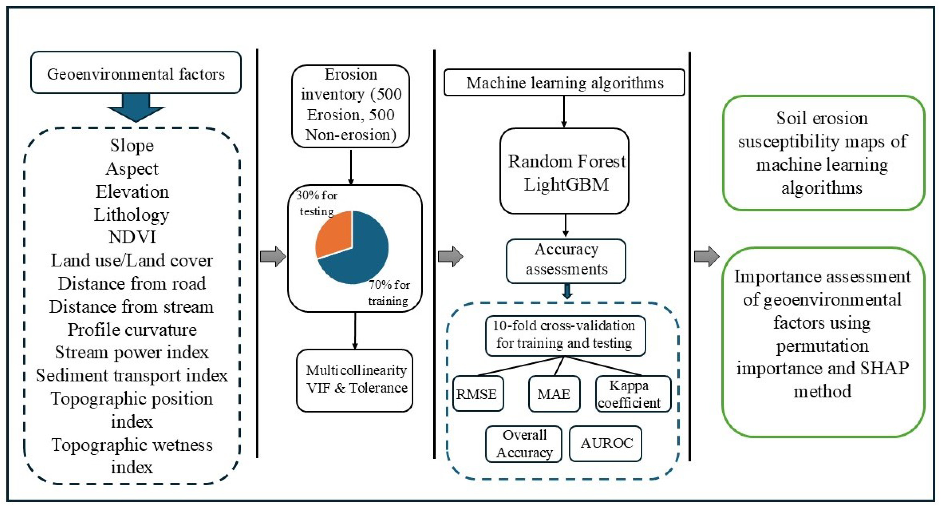
The methodological workflow of this study is illustrated in Figure 2. Initially, thirteen geo-environmental factors considered influential in soil erosion were selected. Erosion-prone locations were identified using high-resolution Google Earth imagery along with field validation. The compiled dataset was then divided into two subsets of 70% for training the machine learning models and 30% for testing their performance. Pearson correlation matrix, Variance Inflation Factor (VIF), and Tolerance (TOL) values were calculated to examine multicollinearity among the input variables. Two machine learning algorithms, including Random Forest and Light Gradient Boosting Machine (LightGBM), were employed to model soil erosion susceptibility. Both LightGBM and Random Forest are tree-based ensemble techniques that are reasonably resistant to overfitting and multicollinearity while handling intricate, non-linear relationships. Their dependability in evaluating soil erosion and land degradation has been established by earlier research [36,37,38]. Additionally, their internal structure makes it possible to extract the importance of features, which makes them appropriate for interpretable modeling, especially when paired with SHAP analysis. The predictive performance of the models was evaluated using several statistical metrics, including Root Mean Square Error (RMSE), Mean Absolute Error (MAE), Kappa coefficient, Overall Accuracy (OA), and the Area Under the Receiver Operating Characteristic Curve (AUROC). These metrics were assessed for both training and testing datasets. Finally, erosion susceptibility maps were generated based on the outputs of the machine learning models. Additionally, permutation importance and Shapley Additive Explanations (SHAP) plots were used to interpret model predictions. They also helped identify the most influential geo-environmental factors contributing to soil erosion mapping in each algorithm.

2.3. Integration of Field Survey and Remote Sensing for Soil Erosion Inventory

A combined approach utilizing field surveys and high-resolution remote sensing data (Google Earth imagery) was employed to develop a spatially accurate inventory of soil erosion. The inventory comprises a balanced set of 1000 points (500 Erosion points, labeled 1; 500 Non-erosion points, labeled 0). The sampling strategy was an expert-driven, non-random approach based on visual interpretation of the available satellite imagery. The high-resolution imagery used for interpretation was sourced from August 2022. Erosion points were specifically labeled based on the presence of visible, concentrated surface features, primarily rills and gullies. Non-erosion sites were confirmed to show no such visible signs of soil loss. Field validation was conducted across representative areas within the study site to verify the potential erosion sites identified remotely. This fieldwork was carried out in April 2023, during which locations were checked in situ, documented with photographs, and uncertain sites were excluded. The main objectives were to verify interpretations and generate reliable ground-truth data. Each digitized point location was used to extract values from the geo-environmental layers, which share a common 12.5 m resolution. Although the initial digitization was manual, the points were distributed across the study area and selected to be spatially independent. This ensured sufficient distance between sampled locations to mitigate autocorrelation. These 1000 points were randomly divided into training (70%) and testing (30%) datasets using a non-spatial split to ensure a balanced and robust model evaluation.

2.4. Geoenvironmental Factors Influencing Soil Erosion Susceptibility

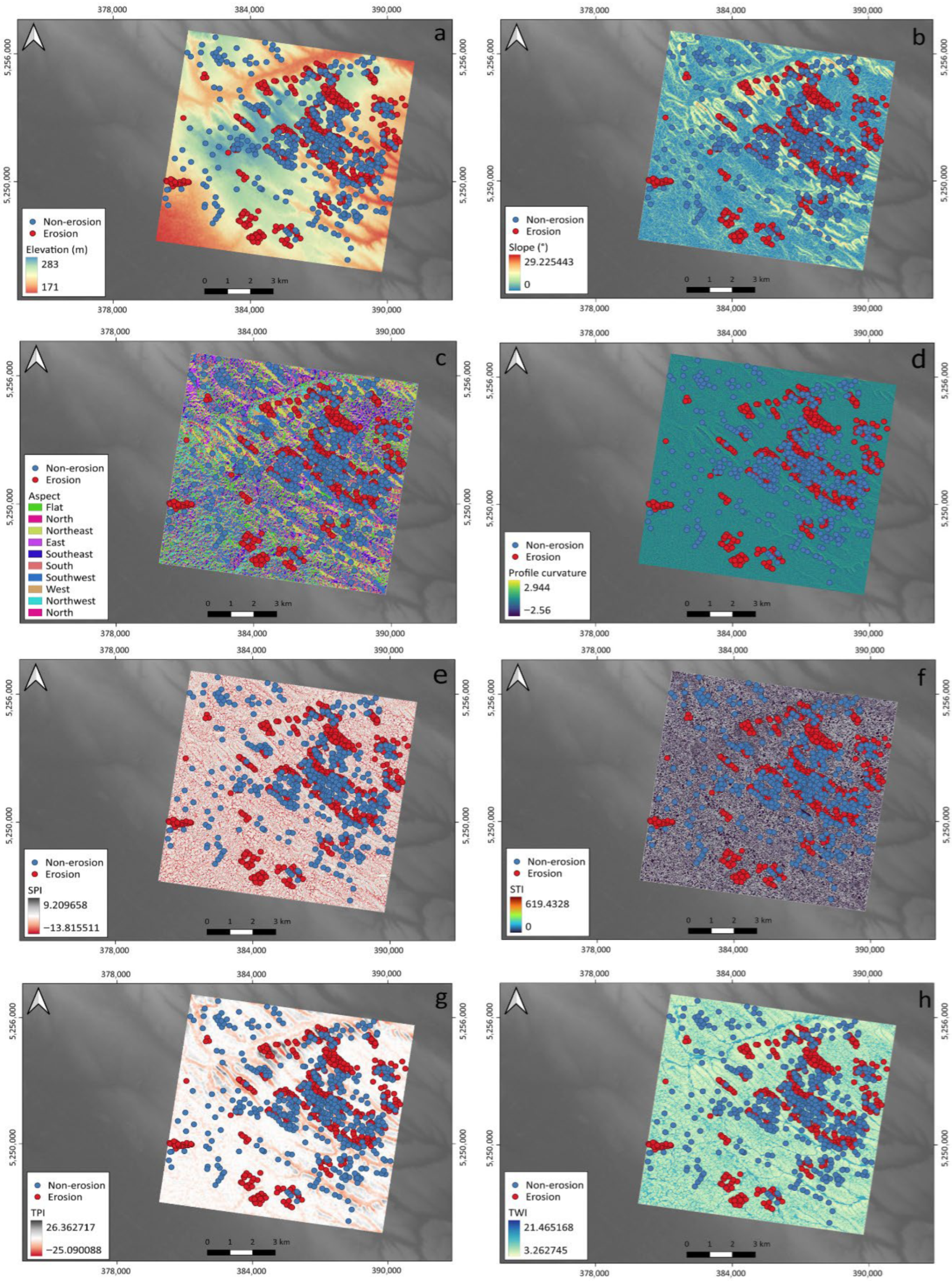
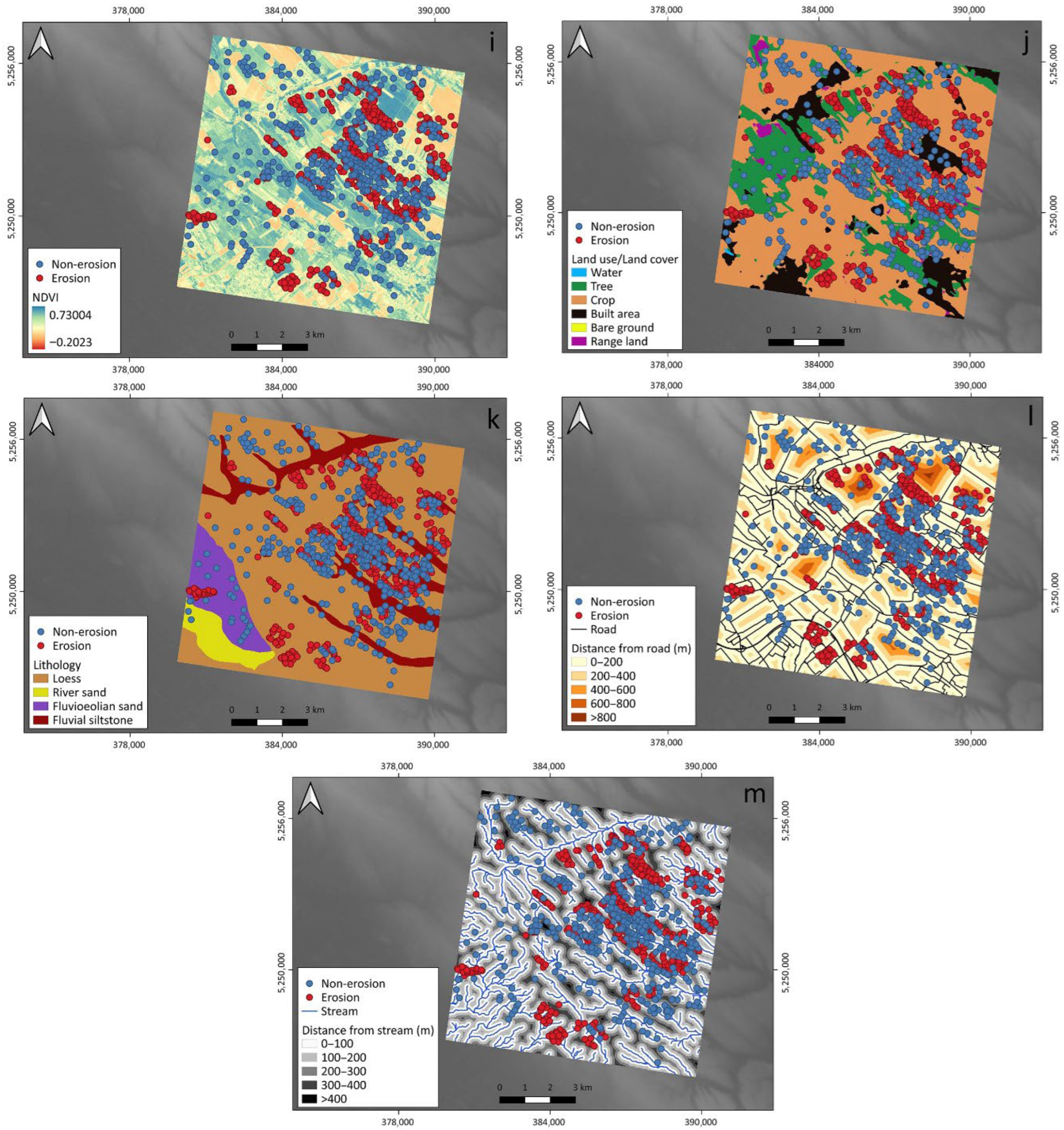
Soil erosion is influenced by a complex interplay of geoenvironmental factors [27,39]. In this study, thirteen factors were selected based on their availability, relevance to erosion processes, and existing knowledge of the study area. We focused exclusively on basic geo-environmental factors (topography, soil, vegetation, and hydrology) because reliable, high-resolution spatial data documenting localized engineering practices (e.g., terracing, contour farming, or crop rotation, which map to the P factor in RUSLE) across the entire study area were unavailable. A detailed description of all factors is provided in Table 1. These include slope, aspect, elevation, lithology, land use/land cover, Normalized Difference Vegetation Index (NDVI), distance from roads, distance from streams, profile curvature, stream power index (SPI), sediment transport index (STI), topographic position index (TPI), and topographic wetness index (TWI). Each factor uniquely affects erosion by influencing surface runoff, soil stability, vegetation distribution, or topographic form. All factor maps were prepared and processed in ArcMap 10.8 and QGIS 3.14.15 (Figure 3a–m). Specifically, slope, aspect, elevation, distance from streams, profile curvature, STI, TPI, TWI, and SPI were derived from a 12.5 m resolution digital elevation model (DEM; https://search.asf.alaska.edu, access date: 27 March 2025). Lithology was obtained from the Hungarian Geological Database (https://map.hugeo.hu/fdt100, access date: 15 March 2025) at a scale of 1:100,000. NDVI was calculated from Sentinel-2 imagery with a 10 m resolution. The image was acquired in May 2022 to reflect the maximum annual vegetation cover. This provides a justified representation of the highest soil protection capabilities during the growing season. Land use/land cover data were acquired from the Pacific Geoportal (https://www.pacificgeoportal.com/, access date: 1 January 2022) with a 10 m resolution. The LULC data utilized a classification defined as follows: Water (class 1), Tree (class 2), Crops (class 5), Built Area (class 7), Bare Ground (class 8), and Rangeland (class 11). Figure 3 shows the maps of all thirteen factors used in the analysis.
To ensure consistency across datasets and enhance model performance, all geoenvironmental layers were resampled to a common resolution of 12.5 m. This reduces computational demand, prevents false precision from unnecessary interpolation, and maintains accuracy. Previous studies have confirmed that grid resolutions between 5 and 20 m are appropriate for deriving reliable terrain parameters in environmental modeling [40,41].

2.5. Multicollinearity Analysis

Before implementing the model, multicollinearity among the input factors was assessed to understand their relationships. This helps reduce the risk of including highly correlated predictors. Addressing multicollinearity helps prevent distortions in model performance and enhances the robustness of the results. When strong collinearity is identified, the associated variable is removed, ensuring an optimal and reliable set of predictive factors [42]. In this study, Pearson’s correlation matrix was employed to assess pairwise relationships between variables, while multicollinearity was further evaluated using Variance Inflation Factor (VIF) and Tolerance (TOL) [2,23,43]. Thresholds commonly used to detect multicollinearity issues are VIF ≤ 10 and TOL ≥ 0.1.

3. Machine Learning Algorithms

In this study, two machine learning algorithms, Random Forest and Light Gradient Boosting Machine (LightGBM), were employed. The machine learning models were executed using Python (version 3.12.7). Using multiple algorithms allows for a comparative analysis of model outputs, facilitating the assessment of their consistency and robustness in predicting soil erosion susceptibility [2].

3.1. Random Forest

Random Forest, introduced by Breiman in 2001 [44], is one of the most widely used machine learning algorithms, particularly valued for its robustness and high predictive accuracy. It was developed to overcome the limitations of individual decision trees by aggregating the results of multiple trees constructed from randomly sampled subsets of the data. As a supervised learning method, Random Forest builds an ensemble of decision trees, each trained on a bootstrap sample of the dataset, with a random subset of features considered at each split [44]. For classification tasks, the final prediction is determined by majority voting across the trees, while in regression tasks, the average of all tree outputs is used [45]. One of this method’s key strengths lies in its ability to reduce overfitting and improve generalization by introducing randomness in both data and feature selection. The model also benefits from using Out-of-Bag (OOB) samples, which are data points not included in the training of a particular tree, to internally estimate prediction error. This offers a built-in validation mechanism that helps assess model performance without the need for a separate validation set [17,20]. These characteristics make Random Forest particularly effective for handling complex, high-dimensional, and non-linear datasets, such as those involved in environmental and geospatial analyses [42]. In this study, the Random Forest model parameters were established based on preliminary stability testing and standard values recognized within environmental modeling literature. The model was trained with n_estimators = 500 (number of trees) to ensure a stable ensemble and robust averaging. Conservative constraints, specifically a max_depth of 10 and a min_samples_leaf of 5, were applied to mitigate the risk of overfitting while maintaining high predictive accuracy.

3.2. Light Gradient Boosting Machine (LightGBM)

LightGBM, introduced by Ke et al. [46], is an advanced gradient boosting decision tree framework designed for high efficiency and scalability. Unlike traditional methods that expand decision trees depth-wise, LightGBM uses a leaf-wise approach, where the leaf with the highest potential to reduce the loss function is split at each iteration. This method results in more compact and computationally efficient trees, improving both performance and memory use. The training process relies on gradient-based optimization to minimize loss functions such as the log loss, commonly used in classification tasks. However, a known limitation of the leaf-wise strategy is its tendency to grow deeper trees, which can lead to overfitting. To mitigate this, LightGBM introduces a maximum depth constraint, which helps balance model complexity and generalization performance [47]. Similarly to the Random Forest model, the LightGBM parameters were chosen based on established practices for controlling model complexity. The model was configured with num_leaves = 10 and a min_data_in_leaf of 20, which are conservative parameters that help control model complexity and prevent overfitting in gradient boosting. A low learnin_rate of 0.02 was used to ensure robust convergence.
Following the implementation of the Random Forest and LightGBM algorithms, erosion susceptibility maps were created for the study area. These maps were classified into five susceptibility categories: Very low, Low, Moderate, High, and Very high, indicating the level of vulnerability to soil erosion. Classification was carried out using the Natural Breaks (Jenks) method in ArcMap 10.8 to ensure optimal grouping of susceptibility values. The final map visualizations and layout arrangements were completed in QGIS 3.14.15.

3.3. Model Performance Evaluation

The performance of each model was evaluated using both the training (70%) and the validation dataset (30%). The data were randomly split into training and validation subsets to ensure a representative distribution of samples across the study area. Root Mean Square Error (RMSE), Mean Absolute Error (MAE), and the Kappa coefficient were computed within a 10-fold cross-validation framework in Python to ensure a robust and reliable assessment of the models’ generalization capability [17,48]. The sample points were well distributed across the study area, which helps minimize the potential influence of spatial autocorrelation and ensures that the models capture the variability of the terrain effectively. Lower values of RMSE and MAE indicate higher accuracy, with values approaching zero representing good performance. The Kappa coefficient ranges from −1 to 1, with values closer to 1 indicating stronger agreement and better model performance [49]. In addition to these measures, Overall Accuracy (OA) and the Area Under the Receiver Operating Characteristic Curve (AUROC) were used for further evaluation. AUROC values range from 0.5 to 1, with higher values reflecting better model accuracy [50]. AUROC values greater than 0.7 are considered acceptable, values above 0.8 indicate excellent predictive capability, and those exceeding 0.9 reflect outstanding model performance [23,51]. Similarly, Overall Accuracy (OA) values closer to 1 indicate more accurate classification results.

3.4. Geoenvironmental Factors’ Importance Evaluation

To assess the contribution of geoenvironmental factors to soil erosion prediction, two interpretability techniques were applied: permutation importance and Shapley Additive Explanations (SHAP) methods. Permutation importance was computed based on the trained Random Forest model, following the approach originally introduced by Breiman [44]. This method evaluates the global influence of each input feature by measuring the decrease in model performance when the values of that factor are randomly shuffled [2]. A substantial drop in accuracy indicates that the variable plays a significant role in the model’s predictions. In addition to this global assessment, SHAP was employed to provide both local and global insights into the model’s behavior. SHAP, which is rooted in cooperative game theory, assigns each factor a Shapley value that reflects its contribution, either positive or negative, to individual predictions [23]. Furthermore, SHAP main effect values [52] were used to quantify the independent impact of each variable.

4. Results

4.1. Correlation Analysis

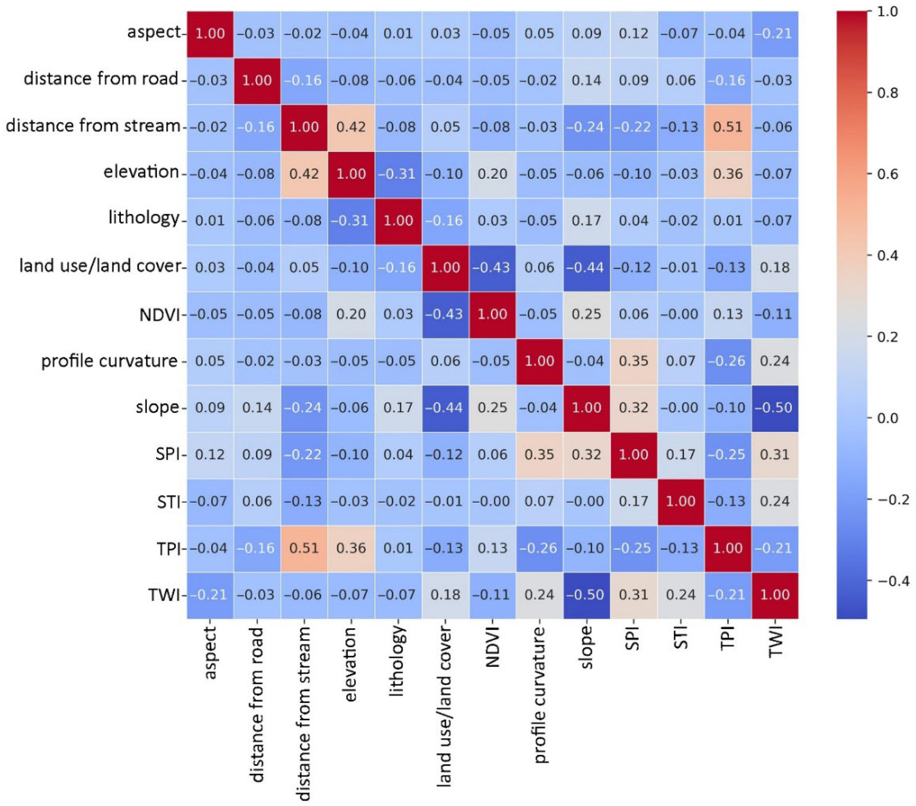
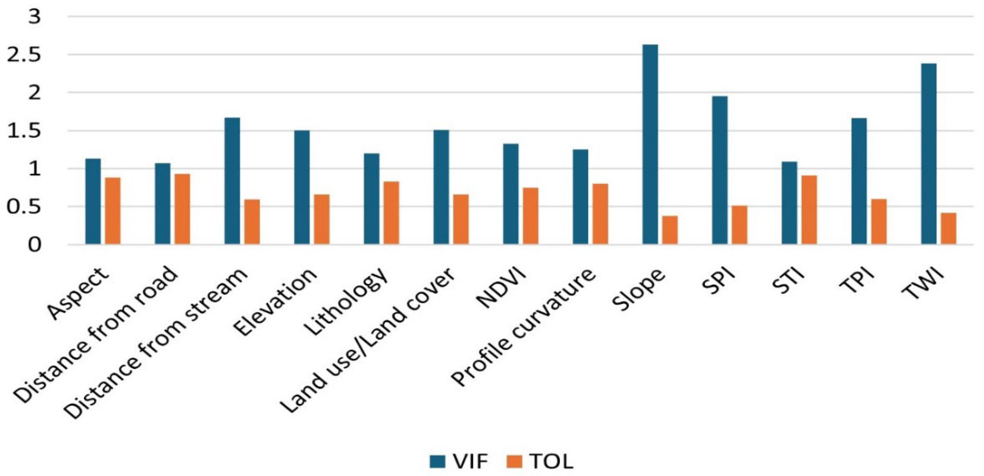
To check for multicollinearity among the geoenvironmental factors, three different methods including Pearson correlation matrix, Variance Inflation Factor (VIF), and Tolerance (TOL) were used. As shown in Figure 4, the correlation matrix reveals a range of positive and negative relationships between the factors. For example, Topographic Position Index (TPI) and elevation show positive correlations with distance from stream, at 0.51 and 0.42, respectively. In contrast, Topographic Wetness Index (TWI) and slope have a negative correlation of −0.50. Similarly, both NDVI and slope are negatively correlated with land use/land cover, with values of −0.43 and −0.44. The highest positive correlation observed was 0.51, while the strongest negative was −0.50. These values suggest that there are no serious correlation issues. VIF values ranged from 1.07 (distance from road) to 2.63 (slope), and TOL values ranged from 0.38 to 0.93 (Figure 5). When Tolerance (TOL) values are greater than 0.1 and Variance Inflation Factor (VIF) values remain well below 10, multicollinearity among the variables can be considered negligible [17,45,53]. Our results met these criteria, confirming that no significant multicollinearity existed among the selected predictors.

4.2. Soil Erosion Susceptibility Mapping and Spatial Variability

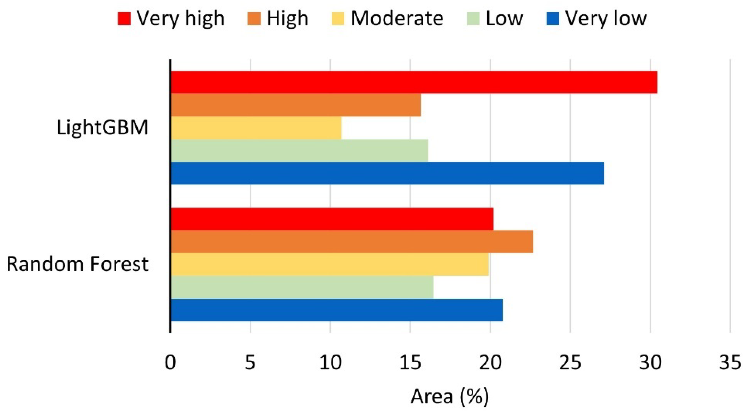
The spatial distribution of soil erosion susceptibility across the study area was assessed using two tree-based machine learning models: Random Forest and LightGBM. As illustrated in Figure 6, both models produced erosion susceptibility maps categorized into five classes: Very low, Low, Moderate, High, and Very high. In both maps, agricultural lands predominantly fall within the High and Very high susceptibility zones, highlighting their vulnerability to water-induced soil degradation. The proportional distribution of each class is presented in Figure 7. According to the Random Forest model, 22.67% of the area was classified as Highly susceptible and 20.2% as Very highly susceptible to soil erosion. In contrast, the LightGBM model predicted a somewhat higher overall risk, with 30.44% of the area categorized as Very high and 15.66% as High susceptibility. The observed variations in class distribution are notable. In particular, LightGBM produces a sharper output, concentrating predictions in the Very High and Very Low classes. In contrast, Random Forest shows a smoother distribution (Figure 7). These differences are likely due to the distinct algorithmic structures of the two models (boosting and bagging). At the lower end of the spectrum, the Random Forest model identified 20.77% of the area as Very low susceptibility, compared to 27.1% estimated by LightGBM. The Low susceptibility class accounted for 16.46% and 16.1% in the Random Forest and LightGBM models, respectively. The Moderate category covered 19.9% of the area according to Random Forest and 10.7% according to LightGBM.

4.3. Spatial Consistency and Models’ Discrepancies

To explain the variations in class distribution, we performed a spatially explicit comparison of the two models. A pixel-wise difference map was generated to identify zones of agreement and divergence (Figure 8). According to the analysis, both models show excellent geographic consistency in stable environments, especially in built-up areas and dense forest covers, where susceptibility is consistently low. However, in some transitional zones, there are significant disparities (probability difference > 20%). These differences are concentrated in agricultural landscapes, particularly those around Mende and Gomba, rather than being random. These discordant zones are characterized by gentle slopes (<5°) and fragmented cropland cover. In these locations, LightGBM consistently predicts higher susceptibility than Random Forest. The statistical distribution depicted in Figure 7 is clearly correlated with this spatial pattern. Only 20.2% of the overall region is classified as Very High susceptibility by Random Forest, compared to 30.44% by LightGBM. In contrast, Random Forest assigns a higher percentage (42%) to the Moderate and High intermediate categories. The structural variations between the algorithms are the cause of this discrepancy. Local forecasts are smoothed by Random Forest’s use of ensemble averaging. As a result, it reduces the susceptibility class to Moderate or High, generalizing the danger over wide agricultural lands. LightGBM, on the other hand, employs a leaf-wise development method. This enables it to identify minor changes in NDVI inside farmed fields as well as local extrema. As a result, LightGBM identifies distinct, high-risk patches within the gentle slopes of the Mende and Gomba regions that Random Forest effectively smooths out.

4.4. Performance Assessment of Random Forest and LightGBM

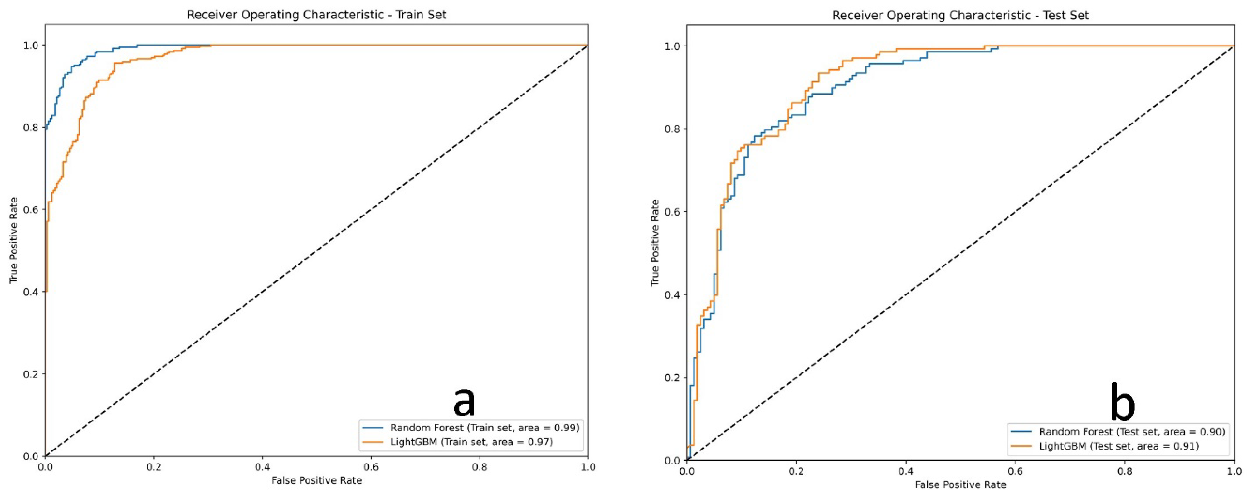
The performance of both Random Forest and LightGBM models was assessed using training and test datasets. During the training phase, Random Forest achieved a slightly higher AUROC score of 0.99, while LightGBM also performed very well with an AUROC of 0.97 (Table 2). However, on the test dataset, LightGBM slightly outperformed Random Forest, with AUROC scores of 0.91 and 0.90, respectively. Additional metrics like the Kappa coefficient and Overall Accuracy (OA) further confirmed the superior performance of the Random Forest model in both datasets. Notably, Random Forest achieved higher Kappa values (0.93 during training and 0.70 during testing) compared to LightGBM (0.85 during training and 0.67 during testing) (Table 2). Similarly, Overall Accuracy (OA) was marginally higher for Random Forest in the training phase (Random Forest: 0.94, LightGBM: 0.9), while both models performed comparably during testing (Random Forest: 0.81, LightGBM: 0.82). Error metrics such as Root Mean Square Error (RMSE) and Mean Absolute Error (MAE) also indicated that Random Forest had lower prediction errors in both training and test datasets. For example, Random Forest recorded RMSE values of 0.18 (train) and 0.38 (test), compared to 0.26 and 0.39 for LightGBM. Similarly, Random Forest achieved smaller MAE values: 0.03 (train) and 0.14 (test), and 0.07 and 0.16 for LightGBM. Figure 9 displays the AUROC for each model.

4.5. Importance Assessment of the Factors

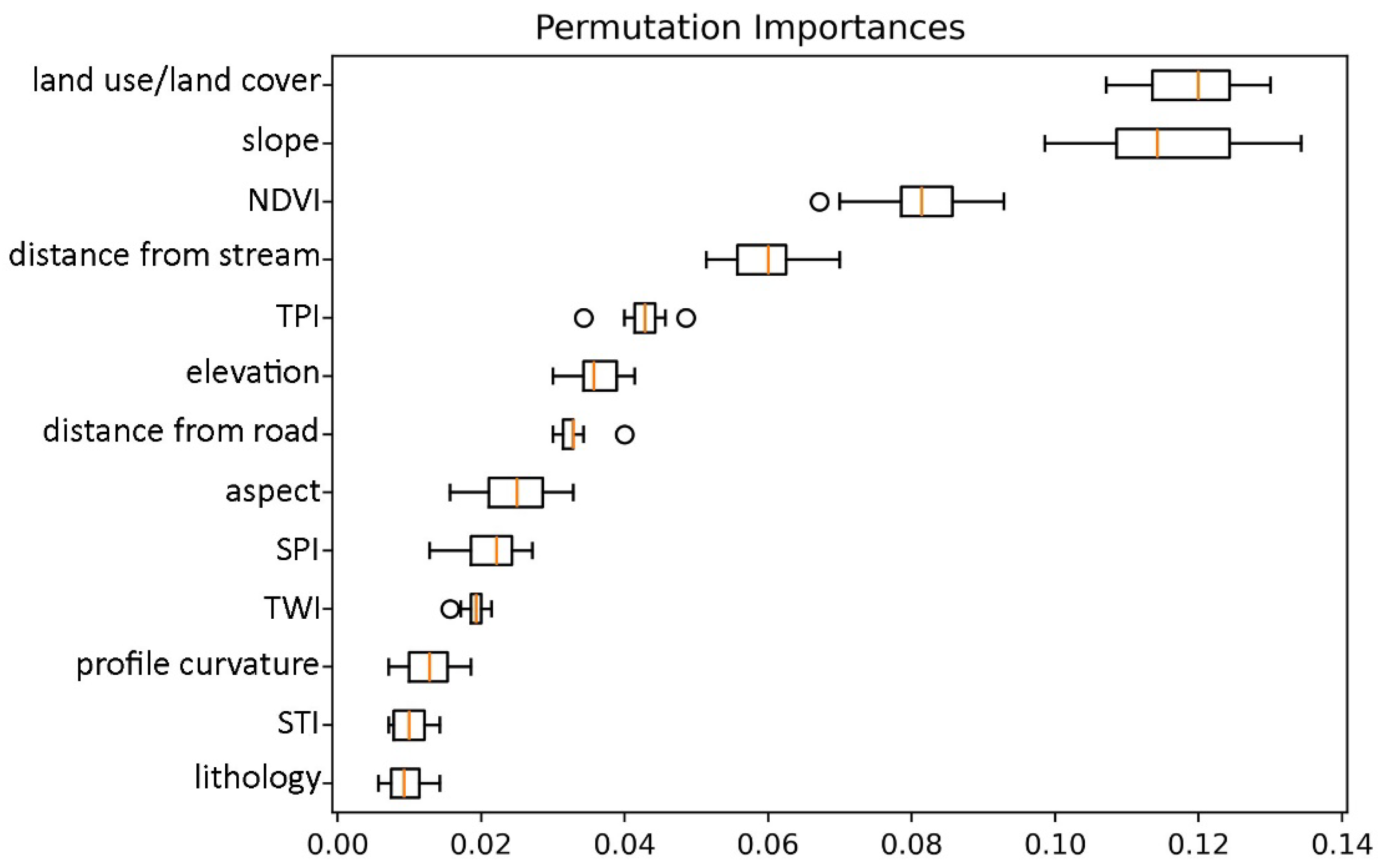
The importance of geo-environmental factors influencing soil erosion was assessed using two interpretability approaches including permutation importance and SHAP (Shapley Additive Explanations). Permutation importance was calculated based on the Random Forest algorithm (Figure 10). According to this method, Land Use/Land Cover (LULC), slope, and the Normalized Difference Vegetation Index (NDVI) emerged as the top three influential factors. These factors play a crucial role in shaping the model’s predictions, emphasizing their significant impact on soil erosion susceptibility.
Figure 11 presents the SHAP summary plots for both the Random Forest and LightGBM models. These plots offer insights into the relative importance of predictors. They also show the direction of their influence, indicating whether a particular factor increases or decreases the model’s output. In the SHAP summary plot for Random Forest (Figure 11a), slope, LULC, and NDVI are confirmed as the most influential variables. The plot shows that lower slope values, higher LULC category values, and lower NDVI values tend to raise erosion susceptibility, indicating a positive contribution to the model’s output. Similarly, the SHAP summary plot for the LightGBM model (Figure 11b) identifies the same three main factors, though in a slightly different order: LULC, slope, and NDVI. The influence and direction of these variables are consistent across both models, with only minor differences in magnitude, demonstrating strong agreement between the two algorithms.
Figure 12 and Figure 13 display the SHAP main effect values, which quantify how different levels of a single variable influence the model’s predictions. SHAP main effects were calculated for all 13 geo-environmental factors across both Random Forest (Figure 12) and LightGBM (Figure 13) models. For conciseness and relevance, the results of the three most significant factors including LULC, slope, and NDVI presented here. Figure 12a depicts the SHAP main effect for slope. The model assigns higher SHAP values to areas with low slope angles, especially below ~5°. This indicates a stronger link to higher erosion risk in flatter terrains. As the slope increases, the SHAP values decrease, suggesting that steeper slopes contribute less to erosion susceptibility. In the LULC SHAP main effect plot (Figure 12b), tree-covered areas (class 2) and built-up areas (class 7) are associated with negative SHAP values, implying a reduced likelihood of erosion in these zones. Conversely, cropland areas (class 5) show positive SHAP values, indicating a greater contribution to erosion risk. Figure 12c presents the SHAP main effect for NDVI. The model detects a clear non-linear pattern where low NDVI values (typically below 0.2), representing sparse or bare vegetation, are strongly linked to higher erosion risk. As NDVI increases, reflecting healthier, denser vegetation, the SHAP values tend toward neutral or negative levels, highlighting vegetation’s protective role in reducing erosion.
Similarly, the SHAP main effect plots for the LightGBM model (Figure 13) further confirm the importance of the same three factors namely LULC, slope, and NDVI. Figure 13a shows the SHAP main effect of LULC. Notably, category 2 (tree-covered areas) and category 7 (built-up areas) exhibit strongly negative SHAP values, indicating a reduced contribution to soil erosion susceptibility in these land cover types. This suggests that such areas are more stable, likely due to vegetation cover in forests and impermeable surfaces or drainage infrastructure in built-up zones. In contrast, category 5 (croplands) is associated with positive SHAP values, implying a higher risk of soil erosion. Figure 13b illustrates the SHAP main effect for slope. The plot indicates that lower slope values, especially below approximately 5 degrees, are linked with positive SHAP values, meaning they contribute more to erosion susceptibility. As the slope increases, the SHAP values decline and become negative, indicating reduced erosion risk on steeper slopes. Figure 13c presents the SHAP main effect for NDVI. The LightGBM model captures a non-linear pattern, where low NDVI values (below ~0.2), indicative of bare or sparsely vegetated surfaces, correspond to high erosion risk, reflected by strongly negative SHAP values. As NDVI increases toward 0.4 and beyond, SHAP values approach zero or become slightly negative, indicating a stabilizing effect of denser vegetation on erosion.

5. Discussion

5.1. Assessment of Multicollinearity Among the Geo-Environmental Factors

The multicollinearity assessment confirmed that there are no serious linear dependencies among the selected geo-environmental factors, supporting the reliability of the model outputs (Figure 4). Although all factors passed the correlation and multicollinearity thresholds, it remains important to consider that moderate correlations might still subtly influence model behavior. The observed positive correlations between the Topographic Position Index (TPI) and elevation with distance from streams (0.51 and 0.42, respectively) reflect expected geomorphological relationships. These indicate that higher terrain features such as ridges or upland zones are typically situated farther from stream networks. Similarly, the moderate negative correlation between slope and the Topographic Wetness Index (TWI) (−0.50) aligns with hydrological logic that steeper slopes generally promote faster surface runoff and reduce moisture accumulation, leading to lower TWI values. The inverse relationships between Normalized Difference Vegetation Index (NDVI) and both slope (−0.43) and land use/land cover (LULC) (−0.44) also offer meaningful ecological insights. Vegetation cover, represented by NDVI, tends to decline on steeper slopes due to shallow soils and increased runoff. The negative correlation with LULC arises from how land cover categories were numerically encoded to facilitate machine learning analysis. Lower numerical values represent more vegetated land types (e.g., category 2 for tree cover, category 5 for cropland), while higher values indicate less vegetated surfaces (e.g., category 7 for built- up areas, category 8 for bare ground). As NDVI values decrease with increasing LULC codes, this coding pattern explains the observed negative correlation. Variance Inflation Factor (VIF) values ranged from 1.07 to 2.63 (below 10), and Tolerance (TOL) values remained above 0.1, confirming that multicollinearity is not a concern (Figure 5) [54].

5.2. Performance of the Machine Learning Algorithms

The performance evaluation of the Random Forest and LightGBM models highlights their strong predictive capabilities for soil erosion susceptibility mapping. Both algorithms demonstrated high accuracy and generalization ability, as evidenced by their performance on both training and test datasets. Random Forest slightly outperformed LightGBM in terms of accuracy and error reduction. However, the differences between the two models were relatively minor. This suggests that both algorithms are well-suited for soil erosion susceptibility mapping. The similar performance of the models across different datasets and evaluation metrics shows that they worked reliably and were not just fitted to the training data. These findings align with Zhang et al. [23] and Gholami et al. [2] that have identified Random Forest as a reliable algorithm for environmental modeling. However, the good performance of LightGBM also shows that it can be a fast and efficient option, especially for large or complex datasets. The outcomes of these two models demonstrate the potential of machine learning in mapping geomorphological hazards and can be useful for future studies on soil erosion risk.

5.3. Mechanistic Interpretation of Model Differences

Although both Random Forest and LightGBM achieved comparable predictive accuracy, their distinct algorithmic foundations are essential for understanding the spatial differences observed in the susceptibility maps. Random Forest is a bagging ensemble, training many independent decision trees on bootstrap samples. This averaging approach inherently reduces variance, which tends to smooth the prediction surface and produce the more balanced class distributions observed across the landscape (Figure 7). In contrast, LightGBM uses a boosting strategy, where each successive tree is trained sequentially to correct the residuals (errors) of the previous one. Its leaf-wise tree growth and gradient-based optimization make it highly sensitive to local variations and extreme patterns. This explains the sharper output seen in Figure 7, where predictions are more heavily concentrated in the Very high and Very low susceptibility zones. These structural differences lead to subtle but meaningful variations in how factors influence model outputs. By integrating SHAP main-effect plots and permutation importance, we confirmed that both algorithms consistently identify slope, LULC, and NDVI as dominant drivers, but they differ in the magnitude and threshold response of each. For instance, LightGBM showed slightly higher SHAP values for slopes below 5 degrees (Figure 13b), suggesting that the boosting process captured sharper, more distinct non-linear responses in gentle terrain. This increased sensitivity to minor changes in slope gradient and local LULC (especially vegetation sparsity, where NDVI below 0.2 exerted a stronger positive contribution in LightGBM) drives the more polarized output. The spatial heterogeneity of these responses fits well with the regional context of the loess-covered study area, where high soil erodibility and intensive agricultural disturbance interact with mild topography. In such environments, Random Forest’s averaging mechanism tends to generalize patterns across transitional areas. In contrast, LightGBM’s sequential learning emphasizes local contrasts such as sharp boundaries between bare soil and tree cover. This behavior reflects the true spatial heterogeneity of the contributing factors.

5.4. Importance of Contributing Factors and Comparative Insights

Figure 10 shows the permutation importance results, highlighting the relative contribution of each geo-environmental factor to soil erosion prediction. As consistently confirmed by the SHAP analysis (Figure 11), land use/land cover (LULC), slope, and Normalized Difference Vegetation Index (NDVI) emerged as the most influential in shaping the model’s output. While these top three factors received the highest importance scores, it is important to note that all input factors contributed to the model’s performance. Even those with lower relative importance play a role in the predictive process, although the machine learning algorithm tends to assign greater weight to factors with stronger statistical relationships in the dataset. For example, although lithology is recognized as a major factor influencing erosion, its relative importance was lower in this analysis. This is especially notable in areas like the study area, where loess dominates. This does not reduce its environmental significance but reflects how the algorithm prioritized other predictors based on their explanatory power within this specific dataset.
A meaningful interpretation of these results requires contextualizing them within the broader scientific field of machine-learning-based erosion modeling. In Hungary, only a few studies have employed similar machine learning methods for assessing soil erosion susceptibility. Among these, the study by Takáts et al. [5] is the closest methodological match, as it uses data-driven models (e.g., Ranger and xgbLinear) to predict erosion in vineyard parcels. Their work indicated that topographic variables, particularly the LS factor, curvature, and MRRTF, were the main predictors in bare-soil vineyard regions, while spectral indices related to vegetation gained importance in more vegetated parcels. This pattern, where vegetation indices become more influential with higher vegetation cover, aligns with our finding that NDVI and LULC strongly influence erosion susceptibility. However, our rankings differ in that vegetation-related variables have an even greater influence here, whereas in the vineyard landscape, topographic derivatives played a larger role because of steeper slopes and different land management practices. Since no other recent machine-learning-based erosion susceptibility studies are available for Hungary, this domestic comparison provides only a limited reference point. Therefore, extending the comparison to methodologically similar studies in other regions is necessary. We selected international studies not because of environmental similarity but because they used comparable machine-learning frameworks, enabling meaningful factor importance comparisons. In many of these studies, the hierarchy of influential predictors varies significantly from what we observe here. Mohammadifar et al. [27], working in southern Iran, found that DEM-derived terrain metrics such as TWI, TRI, TST, slope, and SPI were the most influential predictors, while land use and soil type played a lesser role. Similarly, Khosravi et al. [55] identified elevation, rainfall erosivity, vegetation cover, TWI, and plan curvature as the dominant factors. Investigations in more complex terrains, like those by Huang et al. [56] or Zhang et al. [23], also emphasized elevation, slope length, and proximity to stream networks as the strongest drivers. Compared to these studies, our results show a clear different hierarchy, with vegetation condition (NDVI) and land use patterns (LULC) outweighing terrain-based derivatives. This difference does not reflect methodological inconsistency. Instead, it highlights how machine-learning models are sensitive to the statistical structure of each dataset. These structures depend on land management practices, vegetation distribution, and key disturbance processes in the study area. The similarity between our findings and the vegetation-driven patterns observed in the Hungarian vineyard study by Takáts et al. [5] further supports this interpretation. Overall, linking our results to both the limited Hungarian literature and to international studies with similar methods demonstrates that the importance of factors in machine-learning erosion modeling depends on context. This underscores the need for localized assessments and indicates that interpreting predictor relevance should consider land use, vegetation dynamics, and data characteristics rather than relying solely on factor hierarchies reported from other regional settings.
The Shapley Additive Explanations (SHAP) summary plots for both Random Forest (Figure 11a) and LightGBM (Figure 11b) show that slope, land use/land cover (LULC), and Normalized Difference Vegetation Index (NDVI) are the most important factors in modeling soil erosion susceptibility in the study area. The consistent results across two different machine learning models strengthen the reliability of the findings and agree well with the permutation importance analysis. Examining the SHAP values reveals key patterns: lower slope values tend to have a greater impact on increasing erosion susceptibility. Although this might initially seem counterintuitive, it aligns with the characteristics of the study area, which is a low-relief loess landscape where even gentle slopes can accumulate runoff and contribute to soil erosion due to limited vegetation cover and erosion-prone loess coverage. In such gently sloping terrains, even small gradients can significantly contribute to erosion when combined with other risk factors. The SHAP main effect value plot of slope also indicates that slope values below 5° have a positive influence on the model’s output. Our findings are consistent with the results reported by Wei et al. [57], who observed that slopes with gradients less than 20° experienced soil losses far above tolerable levels, despite the use of conservation practices. They highlighted that gentle slopes can be highly vulnerable to erosion, especially when intensive cultivation is involved. Similarly, Gábris et al. [58] found that in the southern part of the Rakaca Valley in Hungary, 66% of the gullies had developed on gentle slopes. Figure 14 provides direct evidence of erosion processes in the study area. The lighter sections represent loess, which are the areas that faced the most erosion, where the upper soil horizon has already been removed. The darker parts show the erosional channels (rills) through which soil is transported downslope. Soil and sediment accumulation at the valley bottom, where soil thickness was observed to be greater than on the mid- and upper slopes, confirms that topsoil is being redistributed through these channels. These severely eroded zones often occur on gentle slopes and are associated with intensive land use, such as crop production or bare soil, reinforcing the model’s finding that LULC is a key driver of erosion. The SHAP main effect values for LULC further confirm that croplands have a positive contribution to the model’s output.
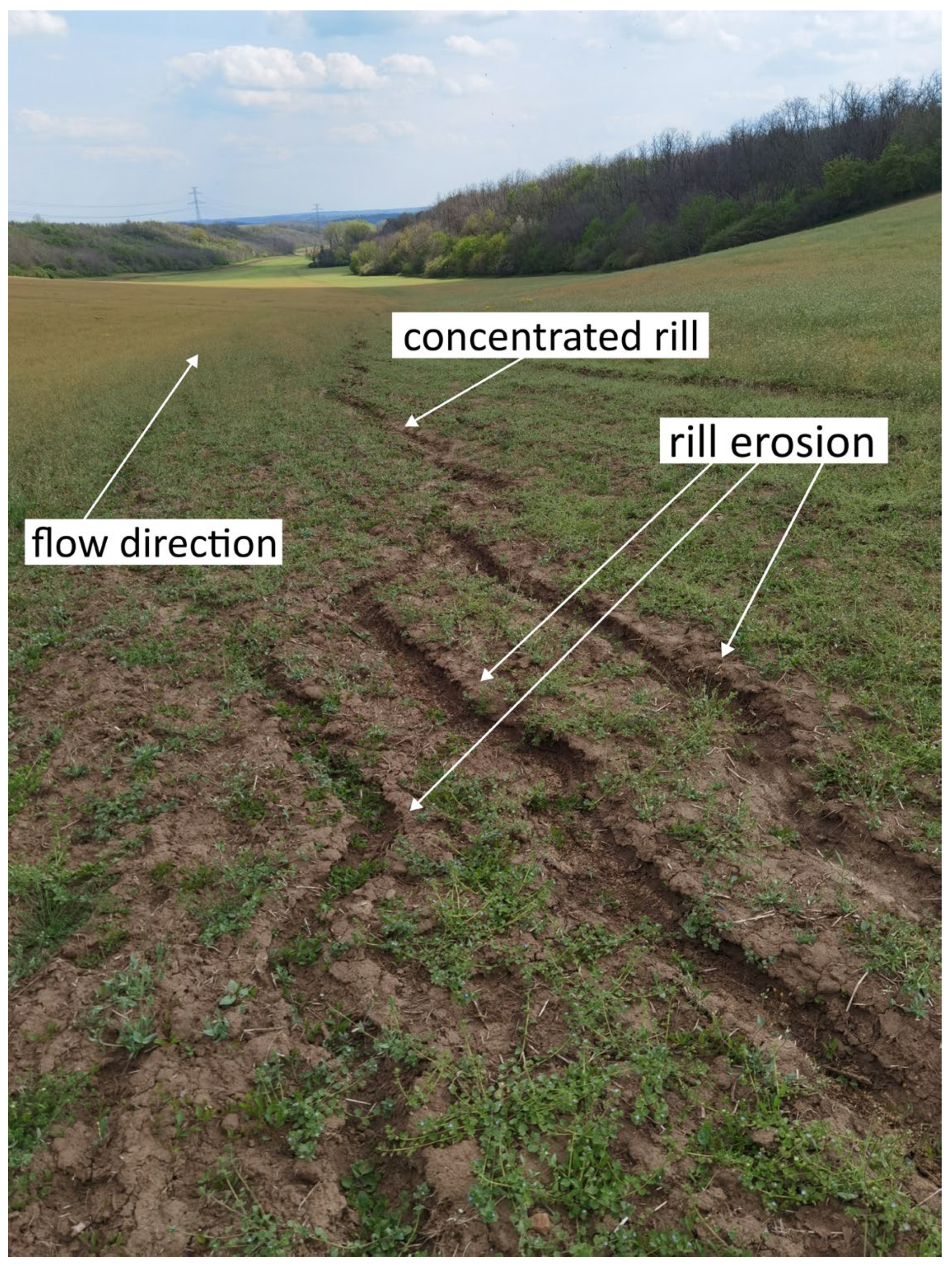
Figure 15 provides further evidence of soil erosion by showing active rill formation on fallow agricultural land with gentle slopes. The image demonstrates the development of concentrated rill networks, which form from surface runoff gathering in areas with sparse vegetation. The effects of plowing are clearly visible, as tillage disrupts the soil structure and increases the risk of erosion. As noted by Gábris et al. [58], rills that form each year on cultivated fields and are temporarily filled by tillage can evolve into ephemeral gullies, contributing significantly to long-term soil degradation in agricultural landscapes. These features not only represent the physical evidence of model predictions but also highlight how topography and land management practices work together to worsen localized soil degradation.
Additionally, Normalized Difference Vegetation Index (NDVI) values show a clear relationship with erosion risk. Areas with low NDVI, which indicates sparse vegetation, are generally more vulnerable to surface runoff and topsoil loss. As shown in the SHAP main effect plot for NDVI, values between 0.1 and 0.3 have a positive influence on the model’s prediction, meaning they are associated with higher erosion susceptibility. Field observations confirm that a lack of vegetation, combined with exposed, tillage-disturbed soil on gentle slopes, significantly contributes to soil loss in agricultural fields. As noted by Manekar et al. [59] continuous tillage, particularly conventional methods, accelerates soil erosion by removing protective crop residues and disrupting soil structure. While erosion is more frequent in poorly vegetated areas, it can also occur in places with relatively dense vegetation, such as forested zones. In some cases, gullies appear to have formed before vegetation developed, but as shown in Figure 16, these gullies remain unstable and continue to evolve. The presence of exposed roots suggests that vegetation has not fully prevented gully development, only may have slowed its progress (Figure 16). These field-based observations highlight the complexity of erosion processes and suggest that erosion is often the result of multiple interacting environmental and land use factors.
Integrating machine learning models with field-based observations provides a robust framework for understanding soil erosion susceptibility in gently sloped, agriculturally active regions. The findings highlight the critical role of land use and vegetation cover in influencing erosion patterns. Importantly, the results offer direct, actionable guidance that the Highly susceptible zones identified should be prioritized for intervention. This necessitates best management practices, such as implementing conservation tillage, ensuring high crop residue coverage (NDVI > 0.4), and establishing grassed waterways, as the primary defense against severe erosion in this low-relief loess environment. These insights reinforce the importance of location-specific erosion control practices that consider both natural and human factors.
While the models showed strong predictive performance, several limitations should be noted. The Normalized Difference Vegetation Index (NDVI) data used in this study represent a single time point and may not capture seasonal variations in vegetation, especially in agricultural areas with crop rotations. Additionally, some input datasets have relatively coarse spatial resolution, which could reduce the accuracy of erosion predictions. Future research could enhance model performance by using higher-resolution remote sensing data, detailed digital elevation models (DEMs), and time-series NDVI to better track changes in land cover over time.

6. Conclusions

Both machine learning algorithms (Random Forest and LightGBM) showed strong predictive performance, with Random Forest having slightly better accuracy and error metrics. The permutation importance and SHAP analyses consistently identified slope, land use/land cover (LULC), and NDVI as the most influential factors affecting soil erosion susceptibility in the study area. The key scientific contribution of this work is the use of Shapley Additive Explanations (SHAP). SHAP helps diagnose and quantify the complex, non-linear influence of these factors. This approach fulfills a critical methodological gap in erosion modeling. Specifically, the SHAP analysis revealed the counter-intuitive finding that lower slope values are most strongly associated with increased erosion susceptibility in the model’s predictions. This quantitative insight confirms that in loess terrains, the high inherent erodibility, coupled with intensive agriculture and sparse vegetation, renders even gentle slopes primary drivers of severe soil loss. By quantifying this specific factor dependency, this study moves beyond simple non-transparent predictions to provide a diagnostic understanding of erosion processes. These results offer actionable insights for land planners, emphasizing the need for targeted erosion control interventions focused on LULC and vegetation management in croplands situated on gentle slopes. Ultimately, this research confirms that integrating interpretable machine learning (SHAP) with field data provides a powerful and necessary framework for sustainable land management in unique geomorphic settings.

Author Contributions

Conceptualization, F.N.N., K.G., Á.N. and E.H.; Data curation, F.N.N.; Formal analysis, F.N.N., K.G., Á.N. and E.H.; Investigation, F.N.N., K.G. and E.H.; Methodology, F.N.N. and K.G.; Software, F.N.N.; Supervision, E.H.; Validation, F.N.N., Á.N. and E.H.; Visualization, F.N.N.; Writing—original draft, F.N.N.; Writing—review and editing, K.G., Á.N. and E.H. All authors have read and agreed to the published version of the manuscript.

Funding

This research received no external funding.

Data Availability Statement

The data that support the findings of this study are available upon reasonable request.

Acknowledgments

We sincerely acknowledge the support of the Stipendium Hungaricum program. This work was also supported by the Hungarian NRDIO K135509 project. We further extend our gratitude to the Alaska Satellite Facility (ASF) for providing the digital elevation model and to the European Space Agency for supplying the satellite imagery utilized in this study. The work of Kaveh Ghahraman was supported by a subsidy from the Polish Ministry of Education and Science for the Institute of Geophysics, Polish Academy of Sciences. We thank the reviewers for their constructive feedback that helped improve this manuscript.

Conflicts of Interest

The authors declare that they have no known competing financial interests or personal relationships that could have appeared to influence the work reported in this paper.

References

  1. Alqadhi, S.; Mallick, J.; Talukdar, S.; Alkahtani, M. An Artificial Intelligence-Based Assessment of Soil Erosion Probability Indices and Contributing Factors in the Abha-Khamis Watershed, Saudi Arabia. Front. Ecol. Evol. 2023, 11, 1189184. [Google Scholar] [CrossRef]
  2. Gholami, H.; Jalali, M.; Rezaei, M.; Mohamadifar, A.; Song, Y.; Li, Y.; Wang, Y.; Niu, B.; Omidvar, E.; Kaskaoutis, D.G. An Explainable Integrated Machine Learning Model for Mapping Soil Erosion by Wind and Water in a Catchment with Three Desiccated Lakes. Aeolian Res. 2024, 67–69, 100924. [Google Scholar] [CrossRef]
  3. Blanco, H.; Lal, R. Principles of Soil Conservation and Management; Springer: New York, NY, USA, 2008; Volume 167169. [Google Scholar]
  4. Shirani, M.; Afzali, K.N.; Jahan, S.; Strezov, V.; Soleimani-Sardo, M. Pollution and Contamination Assessment of Heavy Metals in the Sediments of Jazmurian Playa in Southeast Iran. Sci. Rep. 2020, 10, 4775. [Google Scholar] [CrossRef]
  5. Takáts, T.; Pásztor, L.; Árvai, M.; Gáspár, A.; Mészáros, J. Testing the Applicability and Transferability of Data-Driven Geospatial Models for Predicting Soil Erosion in Vineyards. Land 2025, 14, 163. [Google Scholar] [CrossRef]
  6. van Westen, C.J.; van Asch, T.W.J.; Soeters, R. Landslide Hazard and Risk Zonation—Why Is It Still So Difficult? Bull. Eng. Geol. Environ. 2006, 65, 167–184. [Google Scholar] [CrossRef]
  7. Quyet Nguyen, C.; Thi Tran, T.; Thanh Thi Nguyen, T.; Ha Thi Nguyen, T.; Astarkhanova, T.S.; Van Vu, L.; Tai Dau, K.; Nguyen, H.N.; Pham, G.H.; Nguyen, D.D.; et al. Mapping of Soil Erosion Susceptibility Using Advanced Machine Learning Models at Nghe An, Vietnam. J. Hydroinformatics 2023, 26, 72–87. [Google Scholar] [CrossRef]
  8. Nooshin Nokhandan, F.; Ghahraman, K.; Horváth, E. Erosion Susceptibility Mapping of a Loess-Covered Region Using Analytic Hierarchy Process—A Case Study: Kalat-e-Naderi, Northeast Iran. Hung. Geogr. Bull. 2024, 72, 339–364. [Google Scholar] [CrossRef]
  9. Shen, N.; Wang, Z.; Zhang, F.; Zhou, C. Response of Soil Detachment Rate to Sediment Load and Model Examination: A Key Process Simulation of Rill Erosion on Steep Loessial Hillslopes. Int. J. Environ. Res. Public Health 2023, 20, 2839. [Google Scholar] [CrossRef] [PubMed]
  10. Huang, C.; Hou, X.; Li, H. An Improved Minimum Cumulative Resistance Model for Risk Assessment of Agricultural Non-Point Source Pollution in the Coastal Zone. Environ. Pollut. 2022, 312, 120036. [Google Scholar] [CrossRef]
  11. Echogdali, F.Z.; Boutaleb, S.; Taia, S.; Ouchchen, M.; Id-Belqas, M.; Kpan, R.B.; Abioui, M.; Aswathi, J.; Sajinkumar, K.S. Assessment of Soil Erosion Risk in a Semi-Arid Climate Watershed Using SWAT Model: Case of Tata Basin, South-East of Morocco. Appl. Water Sci. 2022, 12, 137. [Google Scholar] [CrossRef]
  12. Aleksova, B.; Lukić, T.; Milevski, I.; Spalević, V.; Marković, S.B. Modelling Water Erosion and Mass Movements (Wet) by Using GIS-Based Multi-Hazard Susceptibility Assessment Approaches: A Case Study—Kratovska Reka Catchment (North Macedonia). Atmosphere 2023, 14, 1139. [Google Scholar] [CrossRef]
  13. Micić Ponjiger, T.; Lukić, T.; Wilby, R.L.; Marković, S.B.; Valjarević, A.; Dragićević, S.; Gavrilov, M.B.; Ponjiger, I.; Durlević, U.; Milanović, M.M.; et al. Evaluation of Rainfall Erosivity in the Western Balkans by Mapping and Clustering ERA5 Reanalysis Data. Atmosphere 2023, 14, 104. [Google Scholar] [CrossRef]
  14. Bag, R.; Mondal, I.; Dehbozorgi, M.; Bank, S.P.; Das, D.N.; Bandyopadhyay, J.; Pham, Q.B.; Fadhil Al-Quraishi, A.M.; Nguyen, X.C. Modelling and Mapping of Soil Erosion Susceptibility Using Machine Learning in a Tropical Hot Sub-Humid Environment. J. Clean. Prod. 2022, 364, 132428. [Google Scholar] [CrossRef]
  15. Gholami, H.; Mohammadifar, A. Novel Deep Learning Hybrid Models (CNN-GRU and DLDL-RF) for the Susceptibility Classification of Dust Sources in the Middle East: A Global Source. Sci. Rep. 2022, 12, 19342. [Google Scholar] [CrossRef]
  16. Lana, J.C.; Castro, P.d.T.A.; Lana, C.E. Assessing Gully Erosion Susceptibility and Its Conditioning Factors in Southeastern Brazil Using Machine Learning Algorithms and Bivariate Statistical Methods: A Regional Approach. Geomorphology 2022, 402, 108159. [Google Scholar] [CrossRef]
  17. Liu, C.; Fan, H.; Jiang, Y.; Ma, R.; Song, S. Gully Erosion Susceptibility Assessment Based on Machine Learning-A Case Study of Watersheds in Tuquan County in the Black Soil Region of Northeast China. CATENA 2023, 222, 106798. [Google Scholar] [CrossRef]
  18. Bhattacharya, R.K.; Das Chatterjee, N.; Das, K. Modelling of Soil Erosion Susceptibility Incorporating Sediment Connectivity and Export at Landscape Scale Using Integrated Machine Learning, InVEST-SDR and Fragstats. J. Environ. Manag. 2024, 353, 120164. [Google Scholar] [CrossRef]
  19. Bammou, Y.; Benzougagh, B.; Abdessalam, O.; Brahim, I.; Kader, S.; Spalevic, V.; Sestras, P.; Ercişli, S. Machine Learning Models for Gully Erosion Susceptibility Assessment in the Tensift Catchment, Haouz Plain, Morocco for Sustainable Development. J. Afr. Earth Sci. 2024, 213, 105229. [Google Scholar] [CrossRef]
  20. Ghahraman, K.; Nagy, B.; Nooshin Nokhandan, F. Flood-Prone Zones of Meandering Rivers: Machine Learning Approach and Considering the Role of Morphology (Kashkan River, Western Iran). Geosciences 2023, 13, 267. [Google Scholar] [CrossRef]
  21. Gholami, H.; Mohamadifar, A.; Sorooshian, A.; Jansen, J.D. Machine-Learning Algorithms for Predicting Land Susceptibility to Dust Emissions: The Case of the Jazmurian Basin, Iran. Atmos. Pollut. Res. 2020, 11, 1303–1315. [Google Scholar] [CrossRef]
  22. Miller, T. Explanation in Artificial Intelligence: Insights from the Social Sciences. Artif. Intell. 2019, 267, 1–38. [Google Scholar] [CrossRef]
  23. Zhang, W.; Zhao, Y.; Zhang, F.; Shi, X.; Zeng, C.; Maerker, M. Understanding the Mechanism of Gully Erosion in the Alpine Region through an Interpretable Machine Learning Approach. Sci. Total Environ. 2024, 949, 174949. [Google Scholar] [CrossRef]
  24. Lundberg, S.M.; Lee, S.-I. A Unified Approach to Interpreting Model Predictions. Adv. Neural Inf. Process. Syst. 2017, 30, 4765–4774. [Google Scholar]
  25. Cha, Y.; Shin, J.; Go, B.; Lee, D.-S.; Kim, Y.; Kim, T.; Park, Y.-S. An Interpretable Machine Learning Method for Supporting Ecosystem Management: Application to Species Distribution Models of Freshwater Macroinvertebrates. J. Environ. Manag. 2021, 291, 112719. [Google Scholar] [CrossRef] [PubMed]
  26. Li, L.; Qiao, J.; Yu, G.; Wang, L.; Li, H.-Y.; Liao, C.; Zhu, Z. Interpretable Tree-Based Ensemble Model for Predicting Beach Water Quality. Water Res. 2022, 211, 118078. [Google Scholar] [CrossRef]
  27. Mohammadifar, A.; Gholami, H.; Comino, J.R.; Collins, A.L. Assessment of the Interpretability of Data Mining for the Spatial Modelling of Water Erosion Using Game Theory. CATENA 2021, 200, 105178. [Google Scholar] [CrossRef]
  28. Roy, S.; Chintalacheruvu, M.R. Google Earth Engine-Based Morphometric Parameter Evaluation and Comparative Analysis of Soil Erosion Susceptibility Using Statistical and Machine Learning Algorithms in Large River Basins. Earth Sci. Inform. 2024, 17, 75–97. [Google Scholar] [CrossRef]
  29. Emerson, W.W.; McGarry, D. Organic Carbon and Soil Porosity. Soil Res. 2003, 41, 107–118. [Google Scholar] [CrossRef]
  30. Richthofen, F. Reisen Im Nördlichen China: Ueber Den Chinesischen Löss. Verhandlungen Kais.-K. Geol. Reichsanst. 1872, 8, 153–160. [Google Scholar]
  31. Ruszkiczay-Rüdiger, Z.; Fodor, L.; Horváth, E.; Telbisz, T. Discrimination of Fluvial, Eolian and Neotectonic Features in a Low Hilly Landscape: A DEM-Based Morphotectonic Analysis in the Central Pannonian Basin, Hungary. Geomorphology 2009, 104, 203–217. [Google Scholar] [CrossRef]
  32. Pécsi, M. Loess Is Not Just the Accumulation of Dust. Quat. Int. 1990, 7–8, 1–21. [Google Scholar] [CrossRef]
  33. Wu, Q.; Jia, C.; Chen, S.; Li, H. SBAS-InSAR Based Deformation Detection of Urban Land, Created from Mega-Scale Mountain Excavating and Valley Filling in the Loess Plateau: The Case Study of Yan’an City. Remote Sens. 2019, 11, 1673. [Google Scholar] [CrossRef]
  34. Köppen, W. Versuch Einer Klassifikation Der Klimate, Vorzugsweise Nach Ihren Beziehungen Zur Pflanzenwelt. (Schluss). Geogr. Z. 1900, 6, 657–679. [Google Scholar]
  35. Hungarian Meteorological Service. Available online: https://www.met.hu (accessed on 15 March 2025).
  36. Li, H.; Jin, J.; Dong, F.; Zhang, J.; Li, L.; Zhang, Y. Gully Erosion Susceptibility Prediction Using High-Resolution Data: Evaluation, Comparison, and Improvement of Multiple Machine Learning Models. Remote Sens. 2024, 16, 4742. [Google Scholar] [CrossRef]
  37. Oraegbu, A.; Jolaiya, E. Mapping Soil Erosion Classes Using Remote Sensing Data and Ensemble Models. Int. Arch. Photogramm. Remote Sens. Spat. Inf. Sci. 2024, XLVIII-4/W12-2024, 135–142. [Google Scholar] [CrossRef]
  38. Wang, Q.; Tang, B.; Wang, K.; Shi, J.; Li, M. Evaluation of the Gully Erosion Susceptibility by Using UAV and Hybrid Models Based on Machine Learning. Soil Tillage Res. 2024, 244, 106218. [Google Scholar] [CrossRef]
  39. Morgan, R.P.C. Soil Erosion and Conservation; John Wiley & Sons: Hoboken, NJ, USA, 2009; ISBN 1-4051-4467-X. [Google Scholar]
  40. Hengl, T. Finding the Right Pixel Size. Comput. Geosci. 2006, 32, 1283–1298. [Google Scholar] [CrossRef]
  41. Kienzle, S. The Effect of DEM Raster Resolution on First Order, Second Order and Compound Terrain Derivatives. Trans. GIS 2004, 8, 83–111. [Google Scholar] [CrossRef]
  42. Phinzi, K.; Szabó, S. Predictive Machine Learning for Gully Susceptibility Modeling with Geo-Environmental Covariates: Main Drivers, Model Performance, and Computational Efficiency. Nat. Hazards 2024, 120, 7211–7244. [Google Scholar] [CrossRef]
  43. Were, K.; Kebeney, S.; Churu, H.; Mutio, J.M.; Njoroge, R.; Mugaa, D.; Alkamoi, B.; Ng’etich, W.; Singh, B.R. Spatial Prediction and Mapping of Gully Erosion Susceptibility Using Machine Learning Techniques in a Degraded Semi-Arid Region of Kenya. Land 2023, 12, 890. [Google Scholar] [CrossRef]
  44. Breiman, L. Random Forests. Mach. Learn. 2001, 45, 5–32. [Google Scholar] [CrossRef]
  45. Setargie, T.A.; Tsunekawa, A.; Haregeweyn, N.; Tsubo, M.; Fenta, A.A.; Berihun, M.L.; Sultan, D.; Yibeltal, M.; Ebabu, K.; Nzioki, B.; et al. Random Forest–Based Gully Erosion Susceptibility Assessment across Different Agro-Ecologies of the Upper Blue Nile Basin, Ethiopia. Geomorphology 2023, 431, 108671. [Google Scholar] [CrossRef]
  46. Ke, G.; Meng, Q.; Finley, T.; Wang, T.; Chen, W.; Ma, W.; Ye, Q.; Liu, T.-Y. Lightgbm: A Highly Efficient Gradient Boosting Decision Tree. Adv. Neural Inf. Process. Syst. 2017, 30, 52. [Google Scholar]
  47. Wang, D.; Li, L.; Zhao, D. Corporate Finance Risk Prediction Based on LightGBM. Inf. Sci. 2022, 602, 259–268. [Google Scholar] [CrossRef]
  48. Garosi, Y.; Sheklabadi, M.; Conoscenti, C.; Pourghasemi, H.R.; Van Oost, K. Assessing the Performance of GIS- Based Machine Learning Models with Different Accuracy Measures for Determining Susceptibility to Gully Erosion. Sci. Total Environ. 2019, 664, 1117–1132. [Google Scholar] [CrossRef] [PubMed]
  49. McHugh, M.L. Interrater Reliability: The Kappa Statistic. Biochem. Medica 2012, 22, 276–282. [Google Scholar] [CrossRef]
  50. Zabihi, M.; Mirchooli, F.; Motevalli, A.; Khaledi Darvishan, A.; Pourghasemi, H.R.; Zakeri, M.A.; Sadighi, F. Spatial Modelling of Gully Erosion in Mazandaran Province, Northern Iran. CATENA 2018, 161, 1–13. [Google Scholar] [CrossRef]
  51. Hosmer, D.W., Jr.; Lemeshow, S.; Sturdivant, R.X. Applied Logistic Regression; John Wiley & Sons: Hoboken, NJ, USA, 2013; ISBN 1-118-54835-3. [Google Scholar]
  52. Lundberg, S.M.; Erion, G.G.; Lee, S.-I. Consistent Individualized Feature Attribution for Tree Ensembles. arXiv 2018, arXiv:180203888. [Google Scholar]
  53. Lei, X.; Chen, W.; Avand, M.; Janizadeh, S.; Kariminejad, N.; Shahabi, H.; Costache, R.; Shahabi, H.; Shirzadi, A.; Mosavi, A. GIS-Based Machine Learning Algorithms for Gully Erosion Susceptibility Mapping in a Semi-Arid Region of Iran. Remote Sens. 2020, 12, 2478. [Google Scholar] [CrossRef]
  54. Kundu, M.; Ghosh, A.; Zafor, M.A.; Maiti, R. Evaluating the Integrated Performance and Effectiveness of RUSLE through Machine Learning Algorithm on Soil Erosion Susceptibility in Tropical Plateau Basin, India. J. Sediment. Environ. 2024, 9, 665–693. [Google Scholar] [CrossRef]
  55. Khosravi, K.; Rezaie, F.; Cooper, J.R.; Kalantari, Z.; Abolfathi, S.; Hatamiafkoueieh, J. Soil Water Erosion Susceptibility Assessment Using Deep Learning Algorithms. J. Hydrol. 2023, 618, 129229. [Google Scholar] [CrossRef]
  56. Huang, D.; Su, L.; Fan, H.; Zhou, L.; Tian, Y. Identification of Topographic Factors for Gully Erosion Susceptibility and Their Spatial Modelling Using Machine Learning in the Black Soil Region of Northeast China. Ecol. Indic. 2022, 143, 109376. [Google Scholar] [CrossRef]
  57. Wei, W.; Chen, L.; Zhang, H.; Yang, L.; Yu, Y.; Chen, J. Effects of Crop Rotation and Rainfall on Water Erosion on a Gentle Slope in the Hilly Loess Area, China. CATENA 2014, 123, 205–214. [Google Scholar] [CrossRef]
  58. Gábris, G.; Kertész, Á.; Zámbó, L. Land Use Change and Gully Formation over the Last 200 Years in a Hilly Catchment. CATENA 2003, 50, 151–164. [Google Scholar] [CrossRef]
  59. Manekar, U.; Sharma, S.K.; Trivedi, S.K.; Meena, H. Effect of Tillage Management and Soil Slope on Annual Soil Loss Under Cereal Crops in Central India. 2023. Available online: https://pesquisa.bvsalud.org/gim/resource/enauMartinsNetoViviana/sea-229965 (accessed on 3 December 2025).
Figure 1. Location of the study area in Europe (a), Location of the study area within Hungary (b) and spatial distribution of Erosion and Non-erosion points within the study area (c). Red points demonstrate the locations that faced Erosion, and blue points indicate the Non-erosion locations. The points were established using an expert-driven approach based on visual interpretation of high-resolution Google Earth imagery (August 2022), primarily targeting rills and gullies. Sites were field-validated (April 2023) and manually distributed to ensure spatial independence and reliable ground-truth data.
Remotesensing 17 03950 g001
Figure 2. Flowchart of the methodology. NDVI: Normalized Difference Vegetation Index, RMSE: Root Mean Square Error, MAE: Mean Absolute Error, AUROC: Area Under the Receiver Operating Characteristic Curve, SHAP: SHapley Additive Explanations, LightGBM: Light Gradient Boosting Machine.
Remotesensing 17 03950 g002
Figure 3. Selected geoenvironmental factors used in erosion mapping. (a) elevation, (b) slope, (c) aspect, (d) profile curvature, (e) Stream Power Index (SPI), (f) Sediment Transport Index (STI), (g) Topographic Position Index (TPI), (h) Topographic Wetness Index (TWI), (i) Normalized Difference Vegetation Index (NDVI), (j) land use/land cover (LULC), (k) lithology, (l) distance from road, and (m) distance from stream.
Remotesensing 17 03950 g003aRemotesensing 17 03950 g003b
Figure 4. Correlation matrix presenting the strength of relationships among the selected factors (NDVI: Normalized Difference Vegetation Index, SPI: Stream Power Index, STI: Sediment Transport Index, TPI: Topographic Position Index, TWI: Topographic Wetness Index).
Remotesensing 17 03950 g004
Figure 5. Multicollinearity analysis results, indicating acceptable VIF (≤10) and TOL (≥0.1) values for all geoenvironmental factors (NDVI: Normalized Difference Vegetation Index, SPI: Stream Power Index, STI: Sediment Transport Index, TPI: Topographic Position Index, TWI: Topographic Wetness Index).
Remotesensing 17 03950 g005
Figure 6. Soil erosion susceptibility maps generated using Random Forest (a) and LightGBM (b).
Remotesensing 17 03950 g006
Figure 7. Area distribution (%) of soil erosion susceptibility classes derived from Random Forest and LightGBM models.
Remotesensing 17 03950 g007
Figure 8. Spatial distribution of model discrepancies. The map illustrates the pixel-wise absolute difference between the LightGBM and Random Forest susceptibility maps. Red areas highlight zones of disagreement where the difference in susceptibility probability exceeds 20% (absolute difference > 0.2).
Remotesensing 17 03950 g008
Figure 9. Area Under the Receiver Operating Characteristic Curve (AUROC) of two machine learning algorithms using train (a) and test (b) dataset.
Remotesensing 17 03950 g009
Figure 10. Permutation importance chart using Random Forest algorithm (NDVI: Normalized Difference Vegetation Index, TPI: Topographic Position Index, SPI: Stream Power Index, TWI: Topographic Wetness Index, STI: Sediment Transport Index).
Remotesensing 17 03950 g010
Figure 11. SHAP summary plot for both machine learning algorithms. Random Forest (a) and LightGBM (b).
Remotesensing 17 03950 g011
Figure 12. SHAP main effect values from the Random Forest model for the three most important factors: (a) slope, with the horizontal axis showing slope values (degrees); (b) land use/land cover (LULC), with the horizontal axis indicating LULC categories (2: trees, 5: crops, 7: built-up area, 11: rangeland); and (c) Normalized Difference Vegetation Index (NDVI), with the horizontal axis showing NDVI values.
Remotesensing 17 03950 g012
Figure 13. SHAP main effect values of LightGBM algorithm of first three important factors: (a) land use/land cover (LULC), with the horizontal axis indicating LULC categories (2: trees, 5: crops, 7: built-up area, 11: rangeland); (b) slope, with the horizontal axis showing slope values (degrees); and (c) Normalized Difference Vegetation Index (NDVI), with the horizontal axis showing NDVI values.
Remotesensing 17 03950 g013
Figure 14. Erosion in gentle slopes. The lighter surfaces indicate areas where the topsoil has been removed, exposing the underlying loess, while the darker zones represent eroded soil being mobilized and transported downslope through rills. These erosional channels collect eroded materials from slopes and transfer them toward the valley bottom. The fallow agricultural lands, which lack vegetation cover, are more vulnerable to erosion processes (location: near Úri).
Remotesensing 17 03950 g014
Figure 15. Rill erosion occurring on fallow agricultural land with a gentle slope. Individual rills can be seen developing downslope and converging into a concentrated rill channel, highlighting how localized surface runoff can initiate and intensify soil erosion in areas with limited slope variation and sparse vegetation cover (location: near Mende).
Remotesensing 17 03950 g015
Figure 16. Gully erosion with exposed roots indicating ongoing instability of the gully walls. Despite the presence of mature vegetation, the gully continues to widen and deepen. This suggests that vegetation alone may slow erosion, but is insufficient to fully stabilize actively eroding gullies (location: near Felsőfarkasd, Gomba).
Remotesensing 17 03950 g016
Table 1. The details of geo-environmental factors affecting soil erosion.
Geo-Environmental FactorInput SourceUnit/Data TypePhysical Rationale
ElevationALOS PALSAR DEM/12.5 m171–283 m/ContinuousControls potential energy & microclimate
SlopeDerived from DEM/12.5 m0–29.22 degrees/ContinuousGoverns runoff velocity & shear stress
AspectDerived from DEM/12.5 m0–365 degrees/ContinuousInfluences solar radiation & soil moisture
Profile CurvatureDerived from DEM/12.5 m−2.56–2.94/ContinuousAffects flow convergence/divergence
Topographic position index (TPI)Derived from DEM/12.5 m−25.09–26.36/ContinuousIndicates landscape position (ridge/valley)
Topographic wetness index (TWI)Derived from DEM/12.5 m3.26–21.46/ContinuousRepresents potential water accumulation
Stream power index (SPI)Derived from DEM/12.5 m−13.81–9.20/ContinuousIndicates erosive power of concentrated flow
Sediment transport index (STI)Derived from DEM/12.5 m0–619.43/ContinuousRepresents sediment transport capacity
Distance from streamDerived from DEM/12.5 m0 → 400 m/ContinuousIndicates proximity to drainage network base level
LithologyHungarian Geological Database/1:100,000Loess, Rivers sand, Fluvioeolian sand, fluvial siltstone/CategoricalControls erodibility & permeability
Normalized Difference Vegetation Index (NDVI)Sentinel-2 Imagery/10 m−0.2–0.73/ContinuousQuantifies protective vegetation cover
Land use/Land cover (LULC)Pacific Geoportal/10 mWater, Tree, Crop, Built area, Bare ground, Rangeland/CategoricalDefines surface condition & human disturbance
Distance from roadOpen Street Map (OSM)/vector0 → 800 m/ContinuousRepresents potential flow barriers or disturbances
Table 2. Models performance metrics using train and test dataset (RMSE: Root Mean Square Error, MAE: Mean Absolute Error, AUROC: Area Under the Receiver Operating Characteristic Curve).
Train DatasetTest Dataset
Random ForestLightGBMRandom ForestLightGBM
RMSE0.180.260.380.39
MAE0.030.070.140.16
Kappa coefficient0.930.850.700.67
Overall Accuracy0.940.90.810.82
AUROC0.990.970.900.91
Disclaimer/Publisher’s Note: The statements, opinions and data contained in all publications are solely those of the individual author(s) and contributor(s) and not of MDPI and/or the editor(s). MDPI and/or the editor(s) disclaim responsibility for any injury to people or property resulting from any ideas, methods, instructions or products referred to in the content.