Deep Learning-Based Semantic Segmentation for Automatic Shoreline Extraction in Coastal Video Monitoring Systems

Highlights

What are the main findings?

• Deep learning models (U-Net, DeepLabv3+) accurately extracted shorelines from coastal video-monitoring data.
• High boundary F1 scores (up to 0.99) demonstrated the robustness of the proposed methodology.

What are the implications of the main findings?

• Confirms the potential of coastal video-monitoring as a reliable observation tool.
• Provides support for shoreline monitoring in erosion risk assessment and coastal management.

Abstract

Dynamic and vulnerable, coastal zones face multiple hazards such as storms, flooding, and erosion, posing serious risks to populations and ecosystems. Continuous observation of coastal processes, particularly shoreline evolution, is therefore essential. Over the past three decades, coastal video-monitoring systems have proven valuable and cost-effective for studying coastal dynamics. Several approaches have been proposed to determine shoreline position, but each presents limitations, often depending on local conditions or illumination. This study proposes a method based on semantic segmentation using deep neural networks, specifically U-Net and DeepLabv3+ architectures. Both models were trained using time-exposure images from a coastal video-monitoring system, with DeepLabv3+ further evaluated using four convolutional neural network (CNN) backbones (ResNet-18, ResNet-50, MobileNetV2, and Xception). Unlike previous satellite- or UAV-based studies, this work applies deep learning to fixed coastal video systems, enabling continuous and high-frequency shoreline monitoring. Both architectures achieved high performance, with Global Accuracy of 0.98, Mean IoU between 0.95 and 0.97, and Mean Boundary F1 Score up to 0.99. These findings highlight the effectiveness and flexibility of the proposed approach, which provides a robust, transferable, and easily deployable solution for diverse coastal settings.

1. Introduction

Coastal erosion, which affects a significant proportion of sedimentary coastal zones, is a serious issue with potentially significant economic and environmental impacts on communities. Coastal zones are inherently dynamic, undergoing constant transformation due to both natural drivers such as wave activity, rising sea levels, and decreased sediment input from rivers, as well as human-induced pressures including urban expansion and resource exploitation. Within this framework, tracking shoreline location, typically regarded as the interface between terrestrial and marine domains [1], is crucial for analyzing coastal erosion [2], informing management strategies [3], and calibrating numerical simulations [4].

Various methods have been employed to monitor the shoreline, ranging from in situ surveys to remote sensing techniques. Currently, in situ surveys are often conducted using Differential Global Positioning Systems (DGPS) [5], which provide high accuracy but require human resources, incur operational costs, and present limitations in temporal frequency and spatial coverage. Among remote sensing methods, satellite imagery [6], radar [7], lidar [8], video monitoring systems [9], and drones [10] stand out. The selected method depends on the needed resolution in space and time, along with the size of the area to monitor. Nevertheless, surveys conducted with Remotely Piloted Aircraft Systems (RPAS) can also be affected by environmental and operational factors, such as flight height, lighting conditions, and ground control configuration, which influence the accuracy of digital photogrammetry, as reported by [11]. In addition, satellite imagery does not provide sufficient sampling through time of an area of interest to allow applications that require continuous monitoring, and UAV monitoring not only depends on wind conditions but it also depends on the availability of a UAV operator and the associated logistics, per survey epoch. These constraints reinforce the potential of fixed video-monitoring systems combined with deep learning for continuous and fully automated shoreline extraction.

Coastal video monitoring systems have been used since the 1990s for the study of coastal morphodynamic processes, with applications in both scientific and management contexts [9]. These systems offer a practical and low-cost alternative, with easy installation and the capability for continuous data acquisition, providing good spatial and temporal resolutions. Their applications cover a wide range of studies, such as the detection of rip currents [12], longshore currents [13], submerged bar observation [14], topo-bathymetry [15], swash zone delimitation [16], and shoreline detection [17].

Over time, a variety of techniques have been developed to estimate shoreline position within coastal monitoring applications. One of the earliest automated approaches was introduced by Plant and Holman [18], referred to as the Shoreline Intensity Maximum (SLIM), which relies on analyzing time-averaged grayscale images, commonly known as timex (time-exposure) images, a common output of coastal video monitoring systems, created by averaging the video frames from the original footage. Subsequently, several color-based methods were proposed, mainly exploring RGB (Red, Green, Blue) and HSV (Hue, Saturation, Value) color spaces. Some of the most widely used include Pixel Intensity Clustering (PIC) [15], based on pixel distribution analysis, and Colour Channel Divergence (CCD) [19], which relies on divergence between color channels. There are also methods based on edge detection, often requiring manual delineation of a Region of Interest (ROI). To overcome limitations associated with morphological and lighting variability, combined methods integrating several classical techniques have been developed, such as those proposed by Almar et al. [20], Osorio et al. [21], and Ribas et al. [22]. Various strategies utilize machine learning algorithms, for example, artificial neural networks [23] and algorithms based on Structured Support Vector Machines in the CIE 1976 (L*a*b*) color space (CIELAB) color space [24]. Despite their usefulness, these classical approaches are often sensitive to illumination, color variability, and site-specific conditions. In recent years, advances in environmental monitoring technologies, including tomographic, autonomous, and multi-sensor observation systems, have substantially improved the temporal resolution and continuity of coastal observations [25]. These developments have enhanced the capability to monitor shoreline and sediment dynamics in near real time, paving the way for the integration of data-driven and deep learning-based methods.

However, many of these methods still require human intervention, and their effectiveness depends heavily on local conditions, which has encouraged the exploration of more automated and robust approaches, such as those based on deep learning. Some studies rely on edge detection frameworks, such as Holistically-Nested Edge Detection (HED) and its variants [26,27], representing more traditional segmentation approaches. Others combine classical image processing with time-series forecasting [28]. More recently, semantic segmentation architectures, including U-Net, U-Net3+, and DeepLab, have been successfully employed for shoreline extraction from satellite imagery [29,30]. Nevertheless, the application of these techniques to images obtained from fixed coastal video monitoring systems, which offer continuous and high-frequency observations, remains relatively scarce in the literature.

This work explores the application of deep learning-based semantic segmentation to extract shoreline location from imagery captured by a stationary coastal video monitoring system. Recent studies have shown the growing success of deep learning-based semantic segmentation in coastal applications, particularly for shoreline extraction from satellite and video imagery [31,32]. Unlike existing frameworks such as Argus [9] or CoastSnap [33], which rely on pre-established monitoring networks and manual or semi-automatic shoreline detection, this study employs a fully data-driven approach trained on an independently curated dataset from fixed video stations, ensuring full automation and adaptability to local conditions.

Image segmentation involves labeling every pixel in an image according to its category, thereby dividing the image into meaningful regions based on class membership. At a higher level, these elements are often categorized as “things” (discrete and countable objects, such as people, vehicles, or animals) and “stuff” (amorphous and uncountable elements, such as sky, water, or roads) [34]. The most common approaches in the field of segmentation include instance segmentation, semantic segmentation, and panoptic segmentation.

Instance segmentation [35] aims at detecting and segmenting individual objects belonging to the “things” category, producing a distinct mask for each detected instance, without considering “stuff” elements. Semantic segmentation [36], on the other hand, assigns a class label to every pixel, including both ‘things’ and ‘stuff’, without distinguishing separate instances within the same class. Panoptic segmentation [37] merges these concepts, offering both semantic classification and instance-level identification for “things”, while treating all “stuff” pixels of the same class as a single group.

Semantic segmentation has been widely applied, playing a crucial role in various areas such as autonomous vehicles, robotic perception, treatment planning, medical image analysis, and satellite image segmentation. Before the advent of deep learning, several traditional approaches were proposed for semantic segmentation, such as conditional random fields (CRFs) and random forests. Recent advancements in processing capabilities combined with access to extensive datasets have played a key role in accelerating progress in the field of deep learning. In contrast to conventional techniques, methods relying on deep neural networks have demonstrated significantly better results across multiple computer vision challenges, such as semantic segmentation [38,39,40]. Thus, deep learning algorithms have become the dominant approach for segmentation tasks.

Deep learning approaches for segmentation commonly employ Convolutional Neural Networks (CNNs) [41], which consist of convolutional, pooling, and fully connected layers arranged sequentially in order of increasing depth. This structure enables the progressive extraction of features, from simple local patterns to more abstract semantic representations. The introduction of CNNs in semantic segmentation began with Fully Convolutional Networks (FCNs) [39], where the traditional CNN architecture was adapted by replacing the final fully connected layers with convolutional layers, allowing dense, end-to-end segmentation, i.e., pixel-level prediction. Based on FCNs, several variants and improvements emerged, such as SegNet [38] and Pyramid Scene Parsing Network (PSPNet) [42], which introduced more efficient upsampling strategies and global context extraction.

A major breakthrough occurred with U-Net [43], an encoder-decoder architecture composed of two distinct phases: a downsampling (encoder) phase and an upsampling (decoder) phase, connected via skip connections. The encoder captures important features across multiple scales, whereas the decoder rebuilds the segmentation map at a resolution matching that of the original input image. Skip connections concatenate the encoder’s activation maps with the corresponding decoder maps, enabling retention of fine spatial details. This design has become a benchmark for semantic segmentation, especially in medical image analysis, and has found broad application across diverse fields. Building upon this class of encoder–decoder architectures, another widely adopted framework is DeepLab [40], which employs atrous convolutions and Atrous Spatial Pyramid Pooling (ASPP) to enhance multiscale feature extraction and boundary delineation. Subsequent versions introduced additional improvements, with DeepLabv3+ [44] becoming one of the most widely used segmentation networks due to its robustness and versatility.

In this study, we apply deep learning–based semantic segmentation to shoreline detection using coastal video monitoring imagery. Among the available segmentation frameworks, U-Net and DeepLabv3+ were selected due to their wide adoption and complementary design principles. U-Net provides a lightweight encoder–decoder baseline, while DeepLabv3+ incorporates advanced features such as atrous convolutions and multiscale context aggregation. Together, these models allow the evaluation of both efficient and more complex approaches in the context of shoreline detection. To assess their performance in a real-world setting, the methodology was applied to Praia de Mira (Portugal), where the northern sector is backed by a foredune that has undergone severe erosion, threatening nearby residential areas and coastal ecosystems. Recent coastal susceptibility assessments along the adjacent northwestern Portuguese coast have also reported very high to extreme flood and erosion susceptibility levels [45], supporting the high-risk characterization of this area. This context highlights both the scientific and practical relevance of developing robust automated shoreline detection methods for operational monitoring and coastal risk management.

This paper is structured as follows: Section 2 presents the study area, data, and methodology; Section 3 reports the results; Section 4 discusses their implications; and Section 5 concludes with the main findings and perspectives.

2. Methods

2.1. Study Site

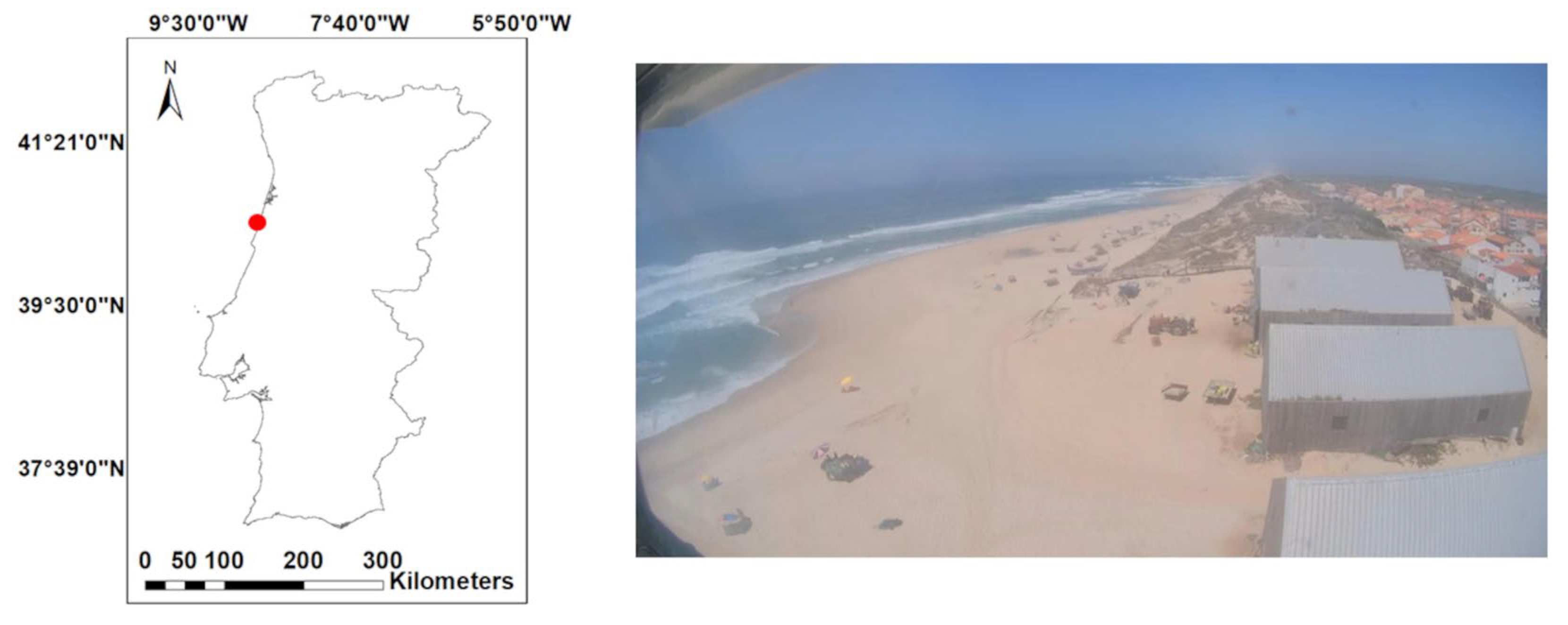
The study site is Mira Beach (40.453°N, 8.804°W), located on Portugal’s exposed western coast (Figure 1, left). This site comprises a sandy beach–dune system directly influenced by North Atlantic wave action. Coastal processes are mainly driven by high-energy wave conditions, with an average significant wave height (Hs) of about 2 m annually and wave periods ranging from 7 to 15 s, predominantly from the west to north-northwest directions. During winter, mean Hs increases to around 3 m, and storm events may generate waves exceeding 8 m [46,47,48]. The tidal regime along this sector of the Portuguese coast is semidiurnal, with a mean tidal range of approximately 2 m (ranging from about 0.6 m at neap tide to 3.2 m at spring tide) [49]. Such conditions highlight the site’s high exposure to energetic forcing, especially during extreme meteorological events that have been associated with episodes of beach erosion and flooding in the region.

The northern sector of Mira Beach is bounded by a foredune ridge, a key geomorphological feature for coastal stability that is particularly vulnerable to erosion during intense storms and spring tides. In some areas, scarping at the dune base has already occurred [50]. This foredune ridge plays a crucial role in protecting nearby residential infrastructure and coastal ecosystems, acting as a natural barrier against wave impact.

2.2. Image Acquisition and Preparation

From October 2019 to June 2023, two HD cameras (1280 × 720 pixels) were deployed at the study site as part of a coastal video monitoring setup, with one camera oriented north and the other south, both positioned 30 m above mean sea level. Each camera continuously recorded 10-min videos at a frequency of 2 Hz during daylight hours. In this study, only data from the north-facing camera were used. The southernmost region was not included in the shoreline extraction due to frequent sun glare affecting image quality. Since it was suspected that these reflections could negatively impact the model’s learning, this region was deliberately omitted from the analysis. Over the course of its operation, this camera acquired a total of 81,020 videos. Figure 1 shows the geographic location of Mira Beach, highlighted with a red dot, and the north-facing camera’s field of view at the site.

Prior to the system’s installation, the camera was calibrated, a process that involves determining its intrinsic parameters, which describe the lens’s internal optical and geometric characteristics [51]. Knowledge of these parameters enables distortion correction and improves the metric accuracy of the acquired images.

Following calibration, image rectification was carried out to correct geometric distortions related to the camera’s orientation, through the estimation of extrinsic parameters that specify the camera’s spatial position and alignment during image capture. This process transforms oblique images into images equivalent to a vertical projection, eliminating distortions caused by camera tilt [52], and is widely adopted in coastal video-monitoring systems [53,54]. This procedure uses control points and photogrammetric methods to model the relationship between three-dimensional ground coordinates (X, Y, Z) and two-dimensional image coordinates (u, v), enabling direct quantitative measurements on the image [52].

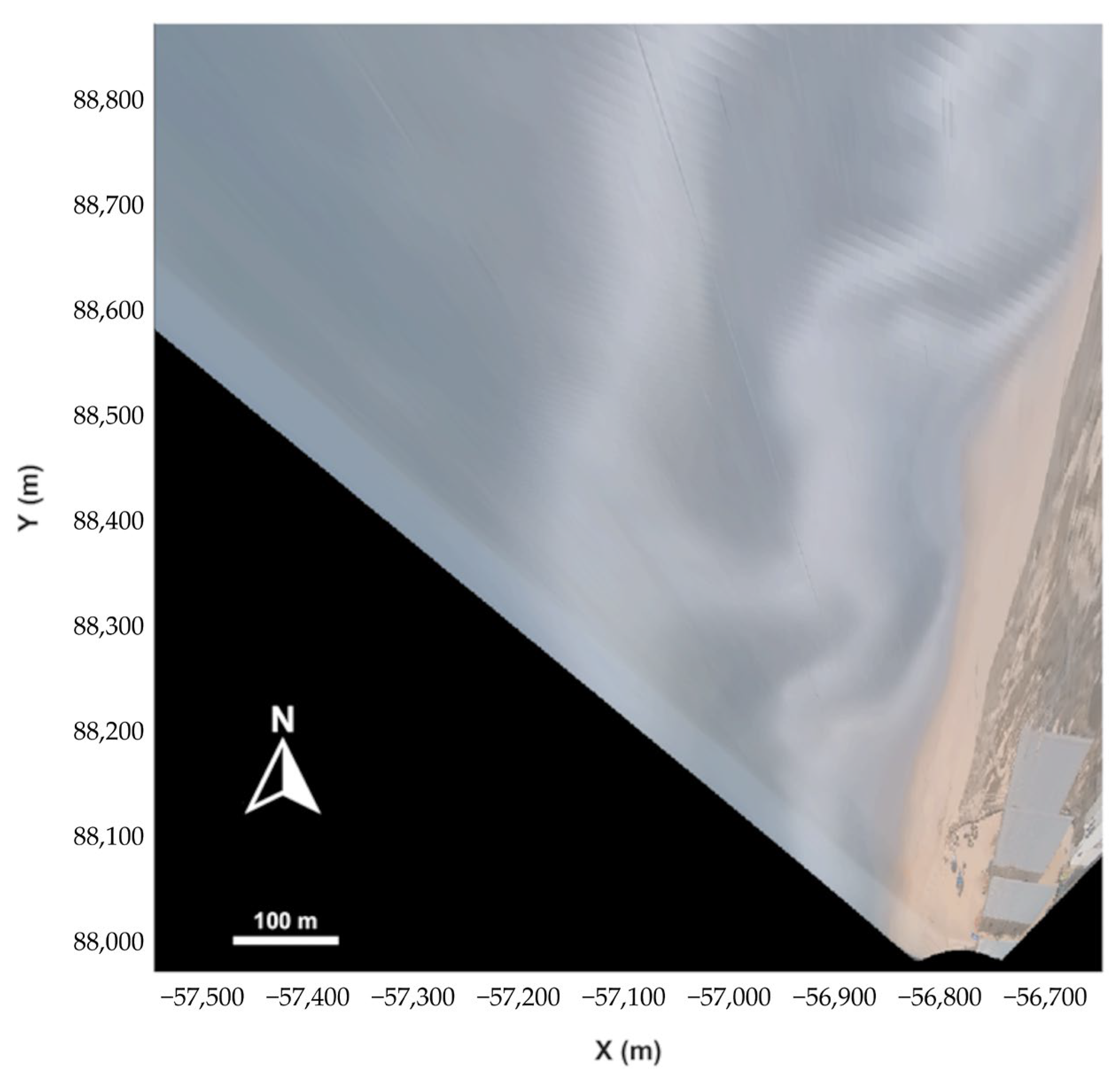
The images were rectified with a spatial resolution of 1 m per pixel and a final dimension of 900 × 900 pixels, corresponding to a ground area of 900 × 900 m, using the PT-TM06/ETRS89 coordinate reference system. The rectification process, based on ground control points, resulted in a root-mean-square error (RMSE) of approximately 0.56 m, which is consistent with the expected accuracy for short-baseline coastal video systems using a limited number of control points. It should be noted that due to the camera’s oblique position and the projection onto a vertical plane, the effective ground resolution (i.e., the area covered by each pixel) decreases with distance from the camera, leading to visible degradation of image sharpness in the more distant regions. Based on the camera geometry, this effect becomes relevant beyond roughly 500–600 m from the camera position, where the projected footprint enlarges noticeably.

This study uses timex images, which are generated by averaging pixel intensities over the entire 10-min duration of each video. This temporal averaging smooths out shoreline oscillations (caused, for example, by wave activity) and lessens interference caused by moving objects visible in the camera’s field, such as boats, people, or vehicles. For these reasons, rectified timex images were selected for this study to enable precise extraction of the shoreline position in metric coordinates. 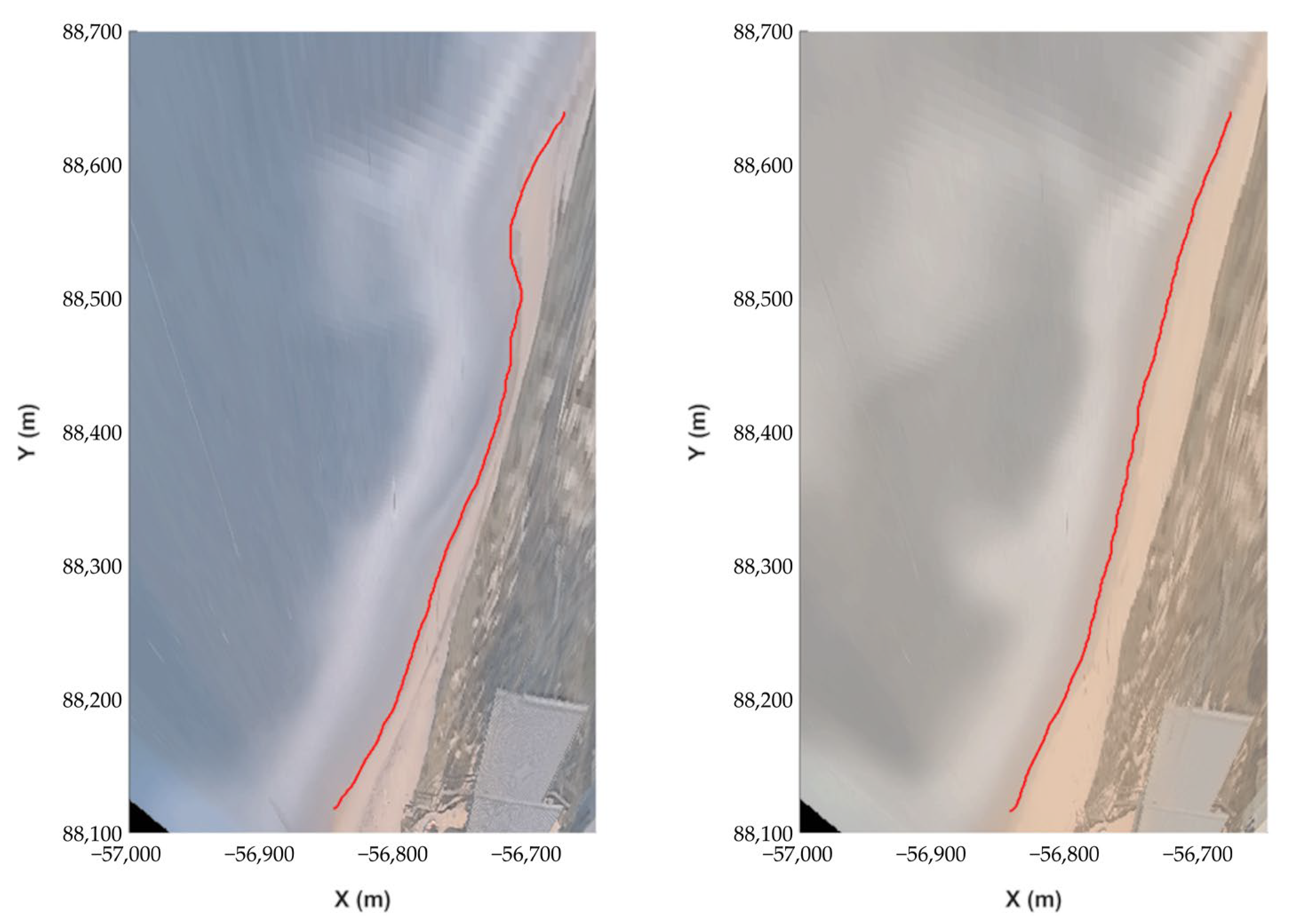Figure 2 presents a rectified timex image.

2.3. Training Dataset Assembly

To ensure a representative and diverse training dataset, a selection of rectified timex images was compiled so that diverse environmental and temporal conditions were well represented. The images reflect different times of day, including transitional periods such as dawn and dusk, as well as varying weather conditions (e.g., clear skies, cloud cover, and light fog) and tidal stages, thereby allowing the shoreline to be observed in multiple positions across the coastal zone.

Images with extremely low visibility, such as those taken during heavy rainfall or dense fog, were excluded. In such cases, the shoreline could not be reliably identified even by human interpretation, thus compromising the quality required for the segmentation task.

The training set consisted of 730 images selected from data acquired between 2019 and 2021, ensuring the inclusion of examples from all months of each year to capture seasonal variations.

2.4. Ground Truth Annotation

Ground truth labels were manually generated using MATLAB 2024a’s Image Labeler application. Two semantic classes were defined: water and sand. The labeling process covered all training images, preserving the original resolution of 900 × 900 pixels to ensure high annotation accuracy along the boundaries between the two classes. As the quality of the segmentation directly affects shoreline extraction accuracy, particular care was taken to produce reliable and detailed ground truth annotations.

Subsequently, a masking operation was applied to remove irrelevant regions of the image and to ensure a balanced proportion of pixels between the two classes. Across the total set of 730 training images, this ratio was kept close to 1 (approximately 1.02), ensuring a balanced sample distribution for each class.

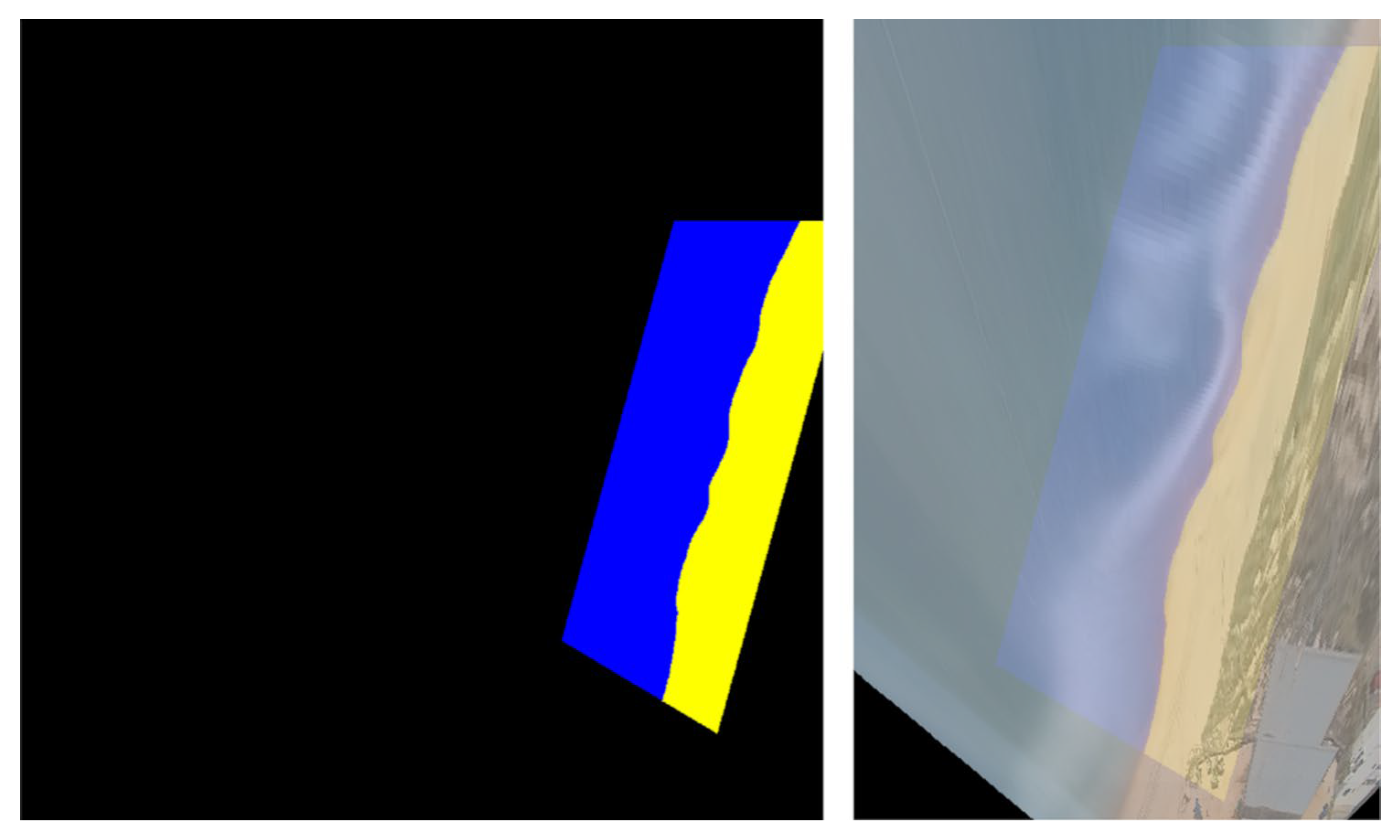
Figure 3 shows an example of a ground truth label at the original resolution of 900 × 900 pixels. The left panel presents the manually annotated segmentation map with the ‘water’ (blue) and ‘sand’ (yellow) classes. The right panel shows the same label overlaid on the corresponding timex image, to illustrate its spatial alignment with the visual scene.

2.5. Model Training

Standard procedures were adopted for training the U-Net and DeepLabv3+ architectures. Each dataset underwent random partitioning, assigning 85% to training and 15% to validation. Before each epoch (i.e., a full pass through the training set), the images were shuffled to randomize their order and prevent learning biases from fixed data sequences. The Adam optimizer [55] was selected because it combines the benefits of momentum and adaptive learning rate methods, making it effective for image segmentation tasks with relatively small datasets. It is also widely used for segmentation problems and showed excellent stability in preliminary trials. Default parameters were used (β₁ = 0.9, β₂ = 0.999, ε = 10⁻⁸), with a fixed initial learning rate of 0.001, which preliminary tests showed to provide stable convergence across models. The loss function adopted was categorical cross-entropy, which evaluates the disparity between predicted class probabilities and true labels, guiding the optimization to minimize classification errors. To mitigate overfitting and improve model generalization, L2 regularization was applied by penalizing large weight magnitudes during training. As the pixel distribution between the two classes was effectively balanced, the use of class weighting strategies was deemed unnecessary.

DeepLabv3+ stands out due to its capability to utilize different convolutional networks as backbone architectures. To assess the impact of backbone choice on segmentation performance, four pre-trained CNNs were evaluated: ResNet-18 and Res-Net-50 [56], MobileNetV2 [57], and Xception [58]. The selection included networks with varying depths, computational complexities, and architectural designs, enabling an analysis of DeepLabv3+ performance across a diverse range of feature extraction strategies, from lightweight and efficient models such as MobileNetV2 to deeper and more sophisticated architectures like Xception. All backbones were initialized with ImageNet pre-trained weights to accelerate convergence and improve generalization, given the limited size of the available training dataset.

For this study, both U-Net and DeepLabv3+ were used with their standard MATLAB 2004a implementations, without any architectural modifications. In the case of DeepLabv3+, the backbones were tested according to their native configurations, while U-Net served as a baseline. The only adjustments concerned input size requirements: 224 × 224 pixels for most architectures and 299 × 299 pixels for Xception. U-Net was also trained with 224 × 224 inputs to ensure comparability. All other architectural settings, including convolutional filter sizes, activation functions, and layer configurations, were kept at their default values. This ensured a consistent basis for comparison while allowing the evaluation of trade-offs between model complexity, training time, and segmentation accuracy.

In addition, U-Net was also tested with 512 × 512 inputs to evaluate the impact of higher spatial resolution.

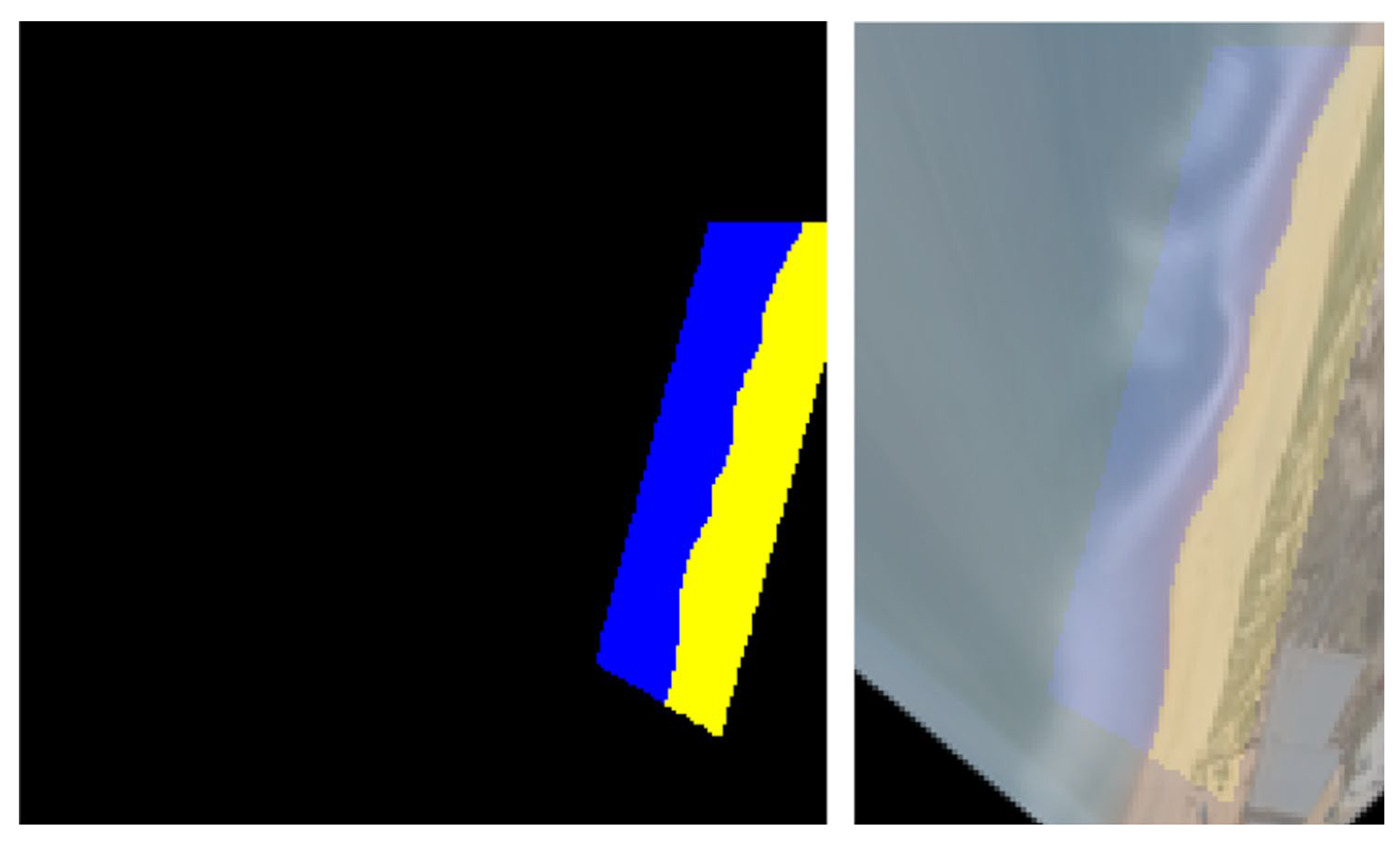
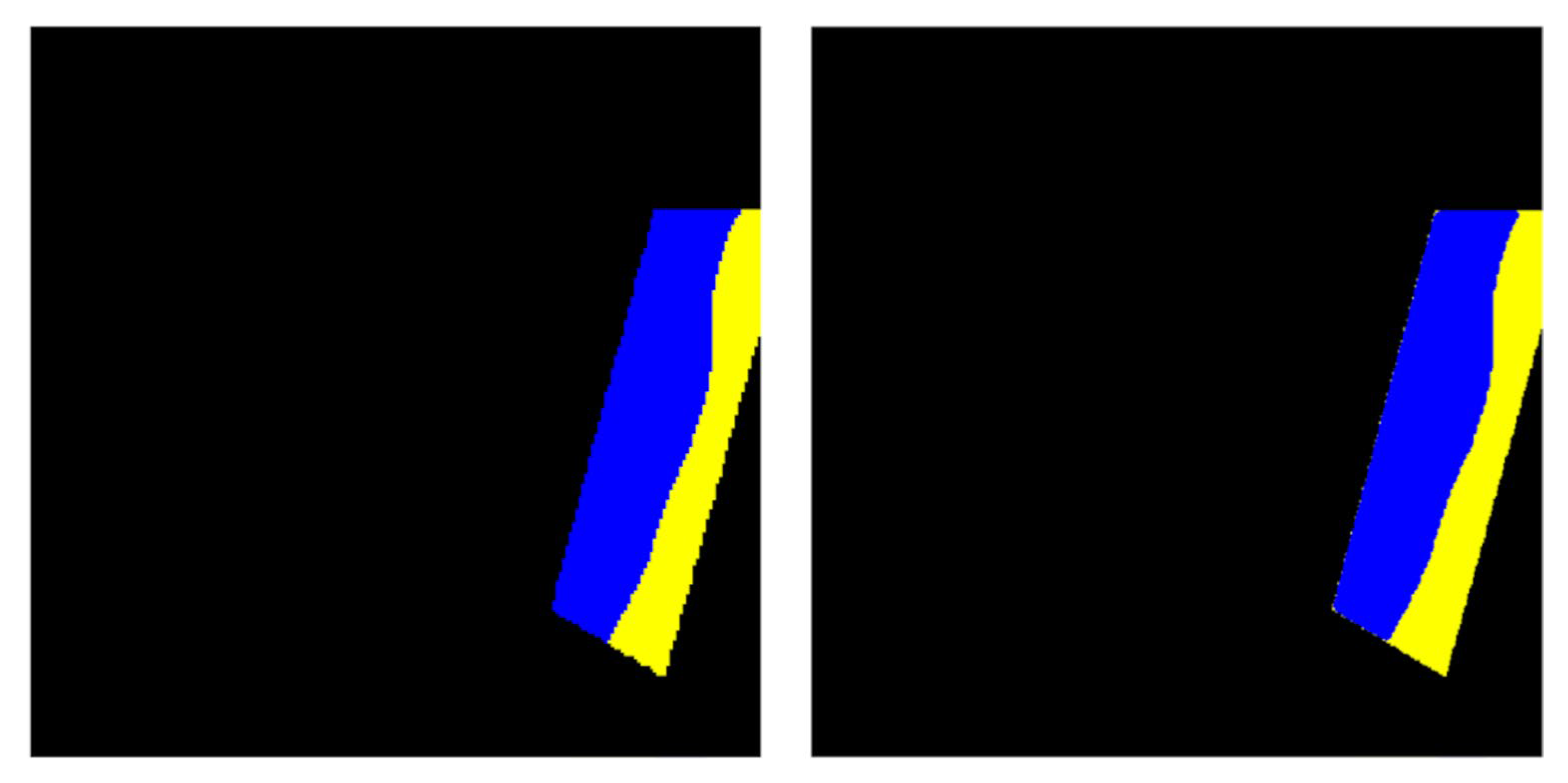
To illustrate the effect of resolution reduction, Figure 4 revisits the example shown in Figure 3, resized to 224 × 224 pixels. The left panel displays the masked ground truth label with the ‘water’ (blue) and ‘sand’ (yellow) classes at this lower resolution, while the right panel overlays it on the corresponding resized timex image. In this example, the reduction from 900 × 900 pixels (1 m/pixel) to 224 × 224 pixels corresponds to an effective sampling of approximately 4 m/pixel.

All training was performed in MATLAB 2024a on a graphics processing unit (GPU) equipped with 8 GB of dedicated video memory, specifically an NVIDIA GeForce RTX 4070 (NVIDIA Corporation, Santa Clara, CA, USA).

2.6. Model Evaluation

To assess model performance, an independent test set of 200 images collected throughout 2022 was used. This ensured temporal independence from the training set (2019–2021) while also providing comprehensive coverage of different times of day, tidal stages, weather conditions, and shoreline morphologies across a complete annual cycle. Although the monitoring system remained operational until mid-2023, those additional five months of data were not included, as the 2022 dataset already provided both seasonal diversity and independence from the training period. As with the training set, ground truth annotations were generated with high precision, ensuring an accurate representation of the shoreline and supporting a consistent and representative evaluation of model performance.

To evaluate the models’ generalization ability and overall effectiveness, the trained networks were tested on the test set, and three metrics were calculated: Global Accuracy, Mean IoU (Intersection over Union), and the Mean Boundary F1 score (Mean BF score). The term mean indicates the average of the metric values computed over the two classes, taking into account all images in the test set.

Global Accuracy corresponds to the proportion of correctly classified pixels relative to the total number of pixels evaluated, and is defined as:

$$Global Accuracy= {\displaystyle \frac{(TP+TN)}{(TP+TN+FP+FN)}}$$

(1)

Mean IoU assesses the agreement between predicted and reference segmentations:

$$IoU= {\displaystyle \frac{TP}{(TP+FP+FN)}}$$

(2)

Finally, the Mean BF score evaluates the alignment of predicted object boundaries with those from the ground truth, providing insight into how accurately the model delineates class contours:

$$BF score={\displaystyle \frac{2\times Precision\ast Recall}{(Precision+Recall)}}= {\displaystyle \frac{2\times TP}{(2\times TP+FP+FN)}}$$

(3)

In these equations, TP, TN, FP and FN denote the true positives, true negatives, false positives, and false negatives. Precision refers to the proportion of correctly identified positive pixels among all pixels predicted as positive, while Recall corresponds to the proportion of correctly identified positive pixels among all actual positive pixels. These definitions follow [39] for Global Accuracy and IoU, and [59] for the BF score.

2.7. Hyperparameter Tuning

Training a neural network requires the adjustment of hyperparameters, such as learning rate, batch size, or the number of epochs, which strongly influence both model accuracy and computational efficiency. Selecting these values is traditionally performed through manual trial and error, but several automated search strategies have been proposed, including grid search, random search, evolutionary algorithms, and Bayesian optimization [60]. No universal method exists, as the effectiveness of each strategy depends on the specific problem, reflecting the principles of the “no free lunch” theorem [61].

In this work, Bayesian optimization [62] was adopted to guide the tuning process. This method iteratively builds a probabilistic model of performance, sampling hyperparameter combinations and selecting the most promising ones for further evaluation. The optimization targeted batch size and number of epochs for both U-Net and DeepLabv3+, while the encoder depth was additionally tested for U-Net. Preliminary experiments indicated that a learning rate of 0.001 ensured stable convergence across models and was therefore fixed. The Mean Boundary F1 Score (BF score) was defined as the objective function, given its sensitivity to shoreline boundary accuracy. Other hyperparameters were tested but had a negligible impact. This strategy allowed systematic exploration of the most influential settings within the limits of the available hardware. The search space included batch size (2–16) and number of epochs (5–20). For the U-Net with 224 × 224 inputs, which also involved testing the encoder depth, the optimization required about 165 iterations, while for the remaining configurations convergence was typically achieved within 80–100 iterations per model.

2.8. Post-Processing and Shoreline Contour Extraction

After semantic segmentation, the resulting segmented images were resized to their original dimensions (900 × 900 pixels) and subjected to a sequence of image processing operations aimed at extracting the shoreline.

To enhance contour extraction, Gaussian smoothing was applied to the binary masks using a kernel with a standard deviation (σ = 2), empirically determined to provide an optimal balance between reducing pixel-level noise and preserving shoreline geometry. This step reduced pixel-level noise and smoothed jagged edges along the class boundaries, a common artifact of discrete segmentation outputs. After smoothing, the masks were re-binarized with a threshold of 0.5, ensuring that class separation was preserved while still benefiting from the reduced edge noise. The final contour was extracted and subsequently transformed into georeferenced shoreline data by converting image-based coordinates into spatial coordinates expressed in meters.

2.9. Exploratory Proof-of-Concept Validation

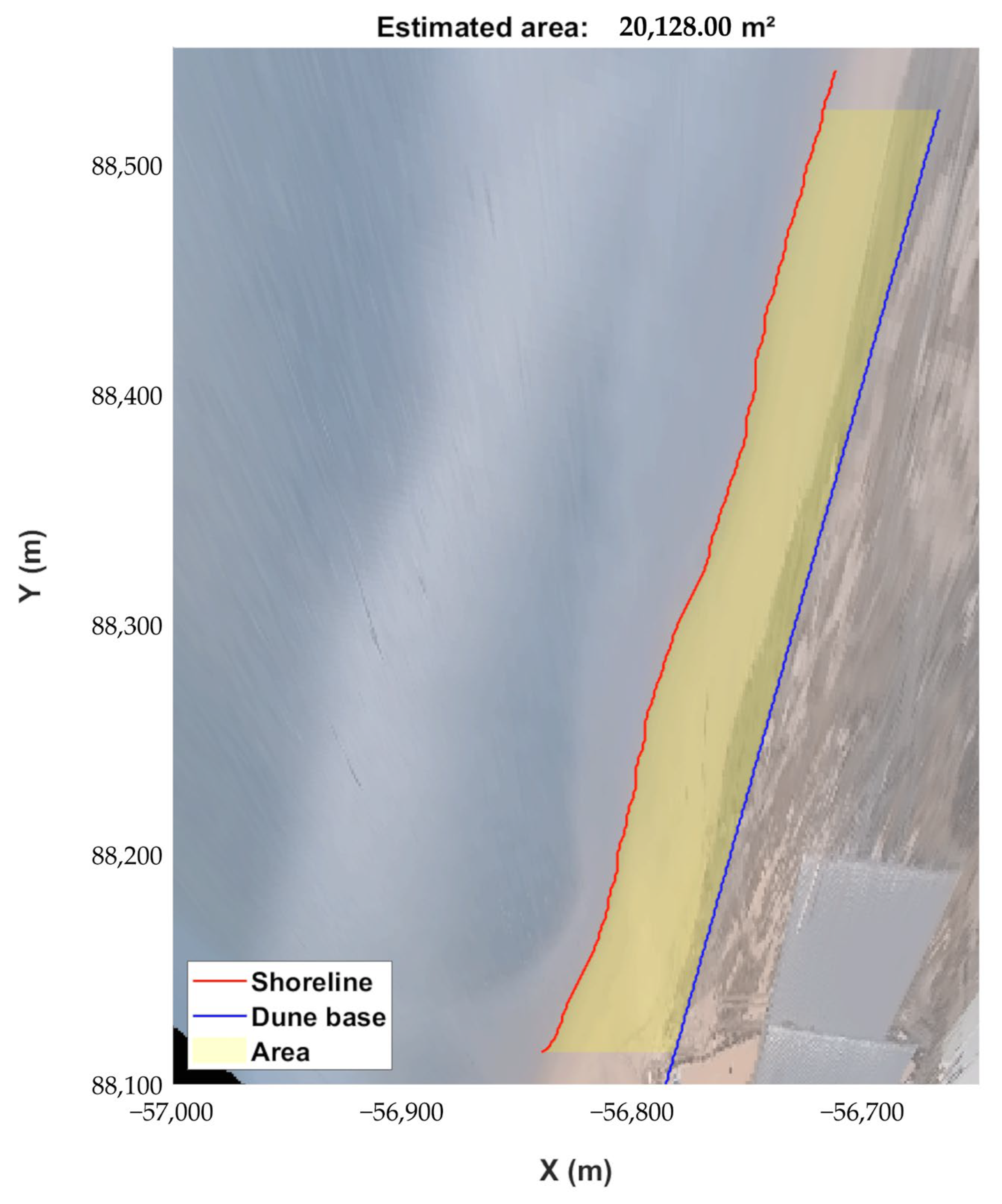
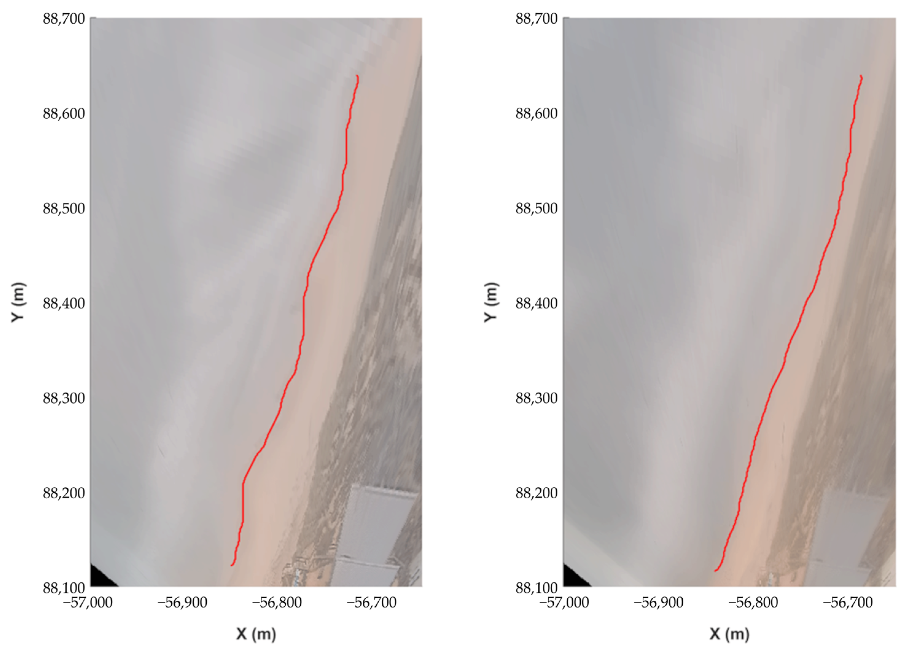
An exploratory proof-of-concept prototype was implemented to test the potential application of the proposed method in an operational context. The system integrated all processing stages from timex image generation to the derivation of spatial metrics. A stationary reference line aligned with the base of the dune, previously surveyed via GPS in 2021 and georeferenced in PT-TM06/ETRS89, was used as the landward limit. This dune baseline was interpolated to ensure point-to-point correspondence with the segmented shoreline. Assuming a flat intertidal topography, beach width was estimated by calculating the Euclidean distance between each point of the segmented shoreline and its homologous point on the dune baseline, defined as the point with the same y-coordinate along the reference line, corresponding to the same cross-shore position. The cumulative sum of these widths provided an estimate of the beach area.

For validation purposes, Sentinel-2 Level-2A imagery (10 m resolution, atmospherically corrected) from 15 dates with good visibility and temporal coincidence with the video data was resampled to 1 m, co-registered with the rectified images, and the shoreline manually delineated using composites derived from the Normalized Difference Vegetation Index (NDVI) and the Normalized Difference Water Index (NDWI), with NDVI proving more effective. The selected images spanned the period from July 2021 to July 2022, covering approximately one year and representing different environmental and tidal conditions. The resulting backshore areas were then compared with those estimated from the video-based system.

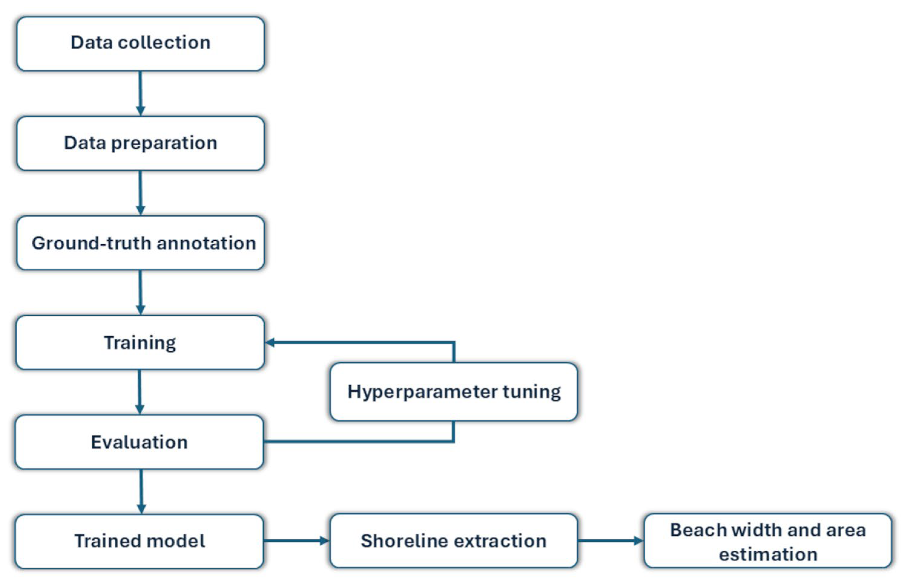
Figure 5 summarizes the overall workflow of the study, illustrating the sequence of steps from data collection to the proof-of-concept validation.

3. Results

Table 1. Performance metrics and training times of the optimized model configurations.

Semantic Segmentation Network	Global Accuracy	Mean IoU	Mean BF Score	Training Time (min)
DeepLabV3+—ResNet18	0.98	0.95	0.98	2.0
DeepLabv3+—ResNet-50	0.98	0.96	0.98	4.1
DeepLabv3+—MobileNet-v2	0.98	0.97	0.99	3.3
DeepLabv3+—Xception	0.98	0.96	0.98	8.3
U-Net (224 × 224)	0.98	0.96	0.98	2.0
U-Net (512 × 512)	0.97	0.95	0.96	40.0

summarizes the performance of the best-performing configurations identified during Bayesian optimization, including evaluation metrics on the test dataset and their corresponding training times. Overall, the models showed consistently high accuracy, while training times varied with architectural complexity.

In addition to the quantitative assessment presented in Table 1, qualitative analyses were conducted to evaluate the visual consistency of the segmentation outputs. Figure 6 illustrates raw and post-processed masks, where Gaussian smoothing was applied to reduce jagged boundaries; in these masks, blue corresponds to water and yellow to sand.

Beyond mask inspection, the extracted shorelines were also evaluated in relation to the original imagery. After resizing predictions to 900 × 900 pixels, the shorelines derived from the processed masks (red lines) were overlaid on the rectified timex images. Figure 7 shows two representative examples, where the extracted shorelines closely match the expected land–water boundary, based on images acquired on 1 July 2021 (left) and 31 March 2022 (right).

To further assess robustness under challenging conditions, Figure 8 presents examples of shoreline extraction during periods of light fog, based on images acquired on 20 December 2021 (left) and 7 April 2022 (right). Even under reduced visibility, the red line representing the extracted shoreline closely follows the apparent land–water boundary in the timex images.

Finally, the prototype implementation was tested to evaluate the practical applicability of the proposed methodology. The complete workflow, from video input and timex image generation to segmentation, contour extraction, and calculation of spatial metrics, was executed within a lightweight framework. Figure 9 shows an example of the spatial metric derived in this proof of concept, based on an image acquired on 13 June 2022, with the estimated beach area (yellow shaded polygon) delineated between the segmented shoreline (red line) and the dune-base reference line (blue line). The comparison with Sentinel-2 imagery resulted in a mean relative error of approximately 8.5%, indicating overall consistency between both approaches. A direct positional comparison (e.g., RMSE of shoreline position) was not performed, since the Sentinel-2 shorelines were manually delineated from 10-m-resolution imagery and resampled to 1 m, which would not provide meaningful spatial accuracy.

4. Discussion

The analysis of the results confirms that all models provided consistently robust performance, with only minor variations across metrics. The high values of Global Accuracy, Mean IoU, and especially the Mean BF score highlight the ability of the proposed approaches to achieve precise shoreline delineation, validating the suitability of deep learning techniques for this type of imagery. Although DeepLabv3+ with MobileNetV2 showed slightly better stability across iterations, the overall conclusion is that both U-Net and DeepLabv3+ variants were equally effective for the segmentation task. This indicates that the choice of backbone, while influencing training times and optimization stability, had only a marginal effect on the final shoreline accuracy.

A key factor that contributed to these results was the adopted preprocessing strategy, particularly the downsampling of images and labels. This simplification sharpened class boundaries and reduced geometric complexity, which facilitated model learning while also alleviating computational demands. Importantly, the subsequent upscaling and post-processing ensured that the final contours remained spatially accurate when compared to the reference. This balance between reduced training complexity and preserved spatial fidelity was central to the robustness of the methodology. However, this strategy also implies that very fine-scale shoreline features may be lost in the process, limiting the applicability of the method when sub-metric precision is required.

In the case of U-Net, the comparison between 224 × 224 and 512 × 512 inputs illustrates the trade-off between spatial detail and computational feasibility. While higher-resolution inputs slightly improved visual richness, they also increased training time and complexity without delivering superior accuracy. Specifically, training time increased from about 2 min to 40 min per run (Table 1), representing a 20× difference, which reinforces the practicality of working with reduced resolutions in real applications, particularly when hardware resources are limited. It also shows that, beyond a certain resolution, additional detail does not necessarily translate into better segmentation, a limitation that is important to acknowledge when considering operational scalability.

A further limitation was the available GPU memory, which led to VRAM overflow when training with 512 × 512 images. This constraint restricted the Bayesian optimization process to only 15–20 iterations per block, significantly reducing the efficiency of hyperparameter tuning. Although several techniques such as gradient accumulation, batch size adjustment, or mixed-precision training can mitigate memory overflow, these were not implemented since the configuration with 224 × 224 inputs already provided stable performance and excellent results. This hardware bottleneck nonetheless illustrates how computational resources can directly influence methodological choices.

Another aspect to note is the limited size of the training dataset (730 images). While relatively small for deep learning standards, the careful selection of representative conditions (e.g., tidal stages, seasonal variability, shoreline shapes, and different weather conditions) likely contributed to the strong generalization capacity of the models. Furthermore, the use of binary masks to exclude irrelevant regions, combined with the near 1:1 ratio between water and sand pixels, simplified the task and reduced the risk of class imbalance, which might otherwise have compromised training stability. These considerations emphasize that the excellent performance achieved was not only a result of the model architectures themselves, but also of deliberate data curation and preprocessing strategies. Although the dataset comprised only 730 images, transfer learning and the balanced representation of diverse shoreline conditions ensured robust learning. The absence of performance degradation when tested on an independent set (including additional unseen images used for the proof of concept) suggests that overfitting was not a limiting factor despite the relatively small training set.

Challenging conditions such as light fog or moderate rainfall exposed some limitations of the approach, with decreased contrast affecting both the models and human interpretation. Nonetheless, the system remained capable of producing meaningful shoreline estimates, indicating robustness under less-than-ideal circumstances. This demonstrates that the methodology can cope with a degree of variability in environmental conditions, though performance naturally decreases with reduced visibility. Future work could address these cases more explicitly, for instance by incorporating temporal information or image enhancement techniques.

Direct comparisons between studies are inherently limited due to differences in data acquisition platforms, spatial resolution, and methodological objectives. Nevertheless, previous works using satellite imagery for shoreline extraction, such as [27,28], have reported overall accuracy values around 95–98% and mean IoU values up to 0.89. Although these studies focused on general segmentation accuracy, the present work emphasizes the precise delineation of the shoreline by adopting the Mean Boundary F1 (BF) Score as a key performance metric. The results obtained demonstrate that the proposed approach, despite relying on consumer-grade video monitoring systems, achieves a level of accuracy comparable or superior to those obtained with high-resolution satellite data, and in line with recent studies such as [30], which achieved F1-scores above 0.95 using hybrid edge-detection and segmentation frameworks.

Beyond methodological validation, the proof of concept demonstrated the potential operational use of the system. The full workflow, encompassing timex generation, segmentation, shoreline extraction, and spatial metric derivation, was completed in under five minutes per video, which is compatible with the system’s continuous 10-min recording cycle. As a preliminary quality check, a simple contrast-to-noise ratio (CNR) analysis was applied to filter out low-visibility images (e.g., dense fog or heavy rain). The CNR was computed for a representative set of clear and low-visibility conditions within the region of interest, and an empirical threshold was defined based on the contrast range observed under favorable illumination. This allowed the automatic exclusion of unsuitable frames before processing, preventing the degradation of segmentation results. The comparison with Sentinel-2 imagery, yielding a mean relative error of 8.5%, further supports the reliability of the approach, despite inherent resolution and interpretation limitations.

Although the results demonstrate high accuracy and consistency, some limitations must be acknowledged. The absence of concurrent topographic surveys prevented a quantitative assessment of absolute positional error; however, the rectification RMSE (≈0.56 m) and the visual agreement with Sentinel-2 shorelines suggest that the total uncertainty is likely below 1 m. In addition, as the model was trained on imagery from a single site, further cross-site validation would be valuable to evaluate its transferability and robustness under different environmental conditions. Future work should also include a quantitative assessment of uncertainty propagation and model sensitivity to factors such as illumination, turbidity, and tidal variability.

Together, these results underline the feasibility of embedding the methodology into coastal monitoring systems capable of issuing timely alerts under critical conditions, while also highlighting that broader validation across multiple sites and longer timeframes will be necessary to fully consolidate its operational readiness. Future extensions could take advantage of open coastal video-monitoring initiatives, such as Argus and CoastSnap, which provide accessible datasets for cross-site validation and method transferability.

5. Conclusions

This study proposed a deep learning–based semantic segmentation approach for automatic shoreline extraction from coastal video-monitoring systems. U-Net and DeepLabv3+ architectures were evaluated, the latter with four different CNN backbones. All models performed consistently well, achieving a Global Accuracy of 0.98, Mean IoU between 0.95 and 0.97, and Mean BF Score up to 0.99. These results demonstrate the robustness and reliability of the proposed methodology, which effectively delineates the land–water boundary while maintaining high spatial fidelity despite the downsampling applied during training.

A proof-of-concept prototype further demonstrated the feasibility of integrating the proposed methodology into an operational framework. The system processed video-derived imagery end-to-end in near real time, delivering shoreline contours and derived spatial metrics based on area comparisons, with a mean relative error of 8.5% when compared with Sentinel-2 estimates. These results highlight the potential of the approach for automated, accurate, and efficient shoreline monitoring with minimal manual intervention.

In the context of Mira Beach, the methodology proved particularly valuable. The site’s foredune ridge plays a critical role in protecting adjacent housing and infrastructure but is highly vulnerable to storm-induced erosion. By providing timely and reliable shoreline estimates, the proposed framework offers an effective tool to support risk assessment and management in this sensitive area.

More broadly, the findings underline the potential of video-based monitoring systems as cost-effective complements to traditional field surveys and remote sensing approaches. Their high frequency of acquisition and relatively low computational demands make them well-suited for integration into coastal management programs. The ability to scale the methodology to other monitored sites enhances its relevance, with clear environmental and economic implications in terms of reducing monitoring costs, supporting early warning systems, and improving decision-making in the face of growing coastal risks.