Article

A Fast Collaborative Representation Algorithm Based on Extended Multi-Attribute Profiles for Hyperspectral Anomaly Detection

Rocket Force University of Engineering, Xi’an 710025, China
*
Author to whom correspondence should be addressed.
Remote Sens. 2025, 17(23), 3857; https://doi.org/10.3390/rs17233857 (registering DOI)
Submission received: 16 October 2025 / Revised: 25 November 2025 / Accepted: 26 November 2025 / Published: 28 November 2025

Highlights

What are the main findings?
  • We use the Extended Multi-Attribute Profile (EMAP) method to extract feature attributes of hyperspectral images, and then replace the sliding dual-window model in collaborative representation with the K-Means clustering algorithm to achieve both higher anomaly detection accuracy and faster detection speed.
  • We experiment on four real hyperspectral datasets and a synthetic dataset, showing that the EMAPKCRD algorithm achieves the highest AUC value among all compared algorithms. Compared with the traditional CRD and its variant RCRD, it not only improves detection accuracy but also shortens the detection time.
What is the implication of the main finding?
  • We address “ignoring spatial features” and “high computational cost” in traditional hyperspectral anomaly detection: EMAP extracts spatial features to enhance anomaly–background distinguishability, and K-means-based background reconstruction reduces complexity, enabling practical engineering applications.
  • We offer a superior technical solution for hyperspectral anomaly detection, whose stable performance in complex scenarios supports “high accuracy and efficiency” demands in military reconnaissance, environmental monitoring, and precision agriculture, with practical application value.

Abstract

As one of the vital research directions in hyperspectral image (HSI) processing, anomaly detection is dedicated to identifying anomalous pixels in HSIs that have significant spectral differences from the surrounding background, and it has attracted extensive attention from numerous scholars in recent years. Anomaly detectors based on collaborative representation have achieved favorable performance in this field. Based on CRD, scholars have proposed many different variants. However, most of these methods only focus on the spectral information of HSIs, and they suffer from slow detection speed and poor robustness. In this paper, we combine the Extended Multi-Attribute Profile (EMAP) with the CRD algorithm, propose a fast collaborative representation anomaly detection algorithm based on the extended multi-attribute profile. First, we use EMAP to extract the spatial structural information of the HSI. Then, before the anomaly detection, we employ the k-means clustering algorithm to separate anomalous pixels with similar features, and obtain a reconstructed background dictionary matrix. This further separates the background from anomalies and improves the robustness of anomaly detection. Finally, we apply a collaborative representation-based anomaly detector to detect anomalies. The proposed method is compared with other algorithms through experiments on four real HSI datasets and one synthetic HSI dataset. The experimental simulation results verify the effectiveness of our proposed method.

1. Introduction

Hyperspectral remote sensing is a terrestrial observation technique grounded in imaging spectroscopy. Its fundamental characteristic is the capability to employ continuous narrow bands with nanoscale spectral resolution, in conjunction with optical spectroscopy, precision sensing, and algorithmic processing, to facilitate continuous multi-channel synchronous observation and spectral data acquisition of surface targets. This technology is crucial in various applications, including land cover identification [1,2], military surveillance [3], agriculture [4], mineral exploration [5], environmental monitoring [3], maritime rescue [6], and other domains [7,8,9,10].
Hyperspectral images are obtained by using spaceborne or airborne imaging spectrometers to conduct uninterrupted scanning of the same ground object within a specific wavelength range [11]. The dimensionality of hyperspectral image data increases exponentially, and the phenomenon of spatial–spectral mixing is pronounced. Typically, the image source comprises a combination of multiple ground spectral features. Hyperspectral imaging has been extensively applied across various remote sensing domains, including classification [12,13], clustering [14,15], unmixing [16], image denoising [17,18], band selection [19,20], change detection [21,22], object detection [23,24], and anomaly detection [25,26]. The technology of hyperspectral anomaly detection is intricate and advanced, necessitating the precise localization of anomalous pixels within complex backgrounds. The primary objective of HAD is to suppress the background while accentuating abnormal targets, with the critical aspect being the identification of characteristic differences between the anomalous target and the background. Hyperspectral images inherently present computational and statistical challenges due to their high-dimensional nature, complexities in modeling intricate backgrounds, and susceptibility to noise interference [27]. Over the past few decades, numerous HAD algorithms have been developed, primarily categorized into those based on statistical conditional assumptions and those grounded in representation theory.
Among the algorithms predicated on statistical assumptions, the RX algorithm [28] and its variants, such as GRX [29] and LRX [30], are particularly notable. These algorithms employ Gaussian distribution models to represent the global background and estimate the probability density function by calculating the background covariance mean, thereby achieving commendable detection performance. Nevertheless, GRX and LRX rely on a dual window model, where the selection of window size poses significant challenges, ultimately undermining the robustness of these methods. To enhance the robustness of the algorithm, Guo et al. introduced a weighted RX anomaly detection algorithm [31], which assigns varying weights to potential anomalies and background samples to more accurately estimate background information. More recently, a CNN-based VAE and RX hyperspectral anomaly detection algorithm [32] has been developed. This algorithm leverages the three-dimensional structural information inherent in hyperspectral images, effectively integrating spectral and spatial data, thereby addressing the limitations of existing detectors that typically rely solely on single-pixel analysis without fully utilizing spatial information.
Methods based on representation theory significantly mitigates the reliance of traditional statistical methods on data distribution assumptions. The fundamental premise of this method is that normal pixels can be approximated as linear combinations of elements within a background dictionary, whereas abnormal pixels cannot be adequately represented by these elements. Consequently, substantial errors may arise during pixel reconstruction, allowing for the detection of abnormal pixels based on the magnitude of the reconstruction error. The anomaly detection algorithm based on collaborative representation is different from other representation theory based algorithms. This method addresses the anomaly separation problem through the lens of linear combination modeling, offering advantages such as simplified implementation and enhanced scalability in handling single-mode problems. The collaborative representation (CRD) [33] algorithm for hyperspectral anomaly detection, introduced by Li et al. stands as a prominent example of algorithms grounded in collaborative representation. This approach posits that each background pixel can be approximated by its neighboring pixels within a sliding dual window centered on the target pixel, thereby facilitating the detection of anomalous pixels while adaptively modeling the background. However, the computational demands of this method limit its widespread application in hyperspectral image anomaly detection. Then, Ma et al. use two elementary transformation matrices corresponding to pixel positions and derived a recursive CRD method using the principle of matrix inversion [34], thereby enhancing detection speed. Furthermore, Wang et al. introduced a hyperspectral image anomaly detector based on ensemble and random collaborative representation (ERCRD), which employs random subsampling of CRD (RCRD) and refines multiple RCRD outcomes through ensemble learning [35]. These two stages constitute an integrated theoretical framework that enhances the precision and stability of anomaly detection algorithms. Additionally, it improves their generalization performance.
Hyperspectral images contain rich spatial information, and effectively leveraging this information can significantly enhance the performance of HSI processing. However, the majority of current anomaly detection methods predominantly emphasize the spectral features of HSI, often neglecting the spatial features. Pesaresi et al. [36] employed the morphological profile (MP) to extract spatial information from high-resolution satellite images. Building on the MP algorithm, Benniktsson et al. [37] introduced extended morphological profiles (EMP), which offer a more precise representation of spatial information. This advancement incorporates more complex morphological operations and more flexible parameter settings, thereby aligning the extracted spatial features more closely with the actual characteristics of the images. Further extending the MP algorithm, Dalla Mura et al. [38] proposed the attribute profile (AP), which models spatial information with greater accuracy than the MP. Owing to the capability to process input images based on various attributes, these images are characterized with considerable dexterity. Consequently, the extended attribute profile (EAP) and EMAP [38] were developed. The EAP is predicated on the utilization of AP to hyperspectral data, while the EMAP represents direct upgradation of EAP in order to encompass multi-attribute scenarios.
In this paper, we combine the Extended Multi-Attribute Profile (EMAP) with the CRD algorithm, proposing a fast collaborative representation anomaly detection algorithm based on the extended multi-attribute profile. The principal contributions of this work are listed below:
  • We utilize EMAP extraction to derive spatial features from HSIs, integrating these with the spatial information inherent in the images to preprocess the hyperspectral data and enhance detection performance.
  • For background reconstruction, we advocate the use of the k-means clustering algorithm post-spatial feature extraction to select representative points for reconstructing background pixels, thereby further augmenting the accuracy of anomaly detection.
  • The reconstructed background matrix, derived from the aforementioned two steps, will serve as the input for the CRD algorithm, facilitating more rapid and accurate anomaly detection results.

2. Related Work

The collaborative representation-based anomaly detection algorithm (CRD) emphasizes the collaborative relationship between dictionary elements. By adopting a sliding dual window strategy, the pixels around the test pixel are linearly combined to obtain the background dictionary matrix X s .
As shown in Figure 1, y i R b × 1 is the pixel to be tested. Centered around the pixel y i , the size of the outer window is w o u t × w o u t , the size of the inner window is w i n × w i n , and the background dictionary matrix X s is the set of linearly arranged pixels between the two windows. X s = x i j = 1 s , s = w o u t × w o u t w i n × w i n .
The goal of the CRD algorithm is to find a weight vector a that minimizes y X s a 2 2 while satisfying the a 2 2 minimum constraint, and its objective function can be expressed as
min a y X s a 2 2 + λ a 2 2 .
where λ is the regularization parameters.
By taking the derivative of a in the above equation and making its derivative zero, we can obtain
a = X s T X s + λ I 1 X s T y .
Considering that pixels in X s that are similar to y i should have larger weights, and pixels that differ significantly from y i should have smaller weights, we therefore added Tikhonov regularization Γ y based on distance weights to adjust the value of the weight vector a . This matrix has a simple and closed solution, and the expression of Γ y is
Γ y = y x 1 2 0 0 y x s 2 .
Then, the objective function can be rewritten as
min a y X s a 2 2 + λ Γ y a 2 2 .
To make the algorithm more stable, we add a constraint of coefficient 1 to the weight vector a . At this point, the objective function is modified to
min a y ^ X ^ s a 2 2 + λ Γ y a 2 2 .
where y ^ = y ; 1 , X ^ s = X s ; 1 . By taking the derivative of a in the above equation, we can obtain
a = X ^ s T X ^ s + λ Γ y T Γ y 1 X ^ s T y ^ .
The degree of pixel anomalies is evaluated by determining the residuals during the reconstruction process
e = y y ^ 2 = y X s a 2 .
where y ^ = X s a is the reconstructed pixel, and when e is greater than the given threshold, the tested pixel is considered abnormal.

3. The Proposed EMAPKCRD Method

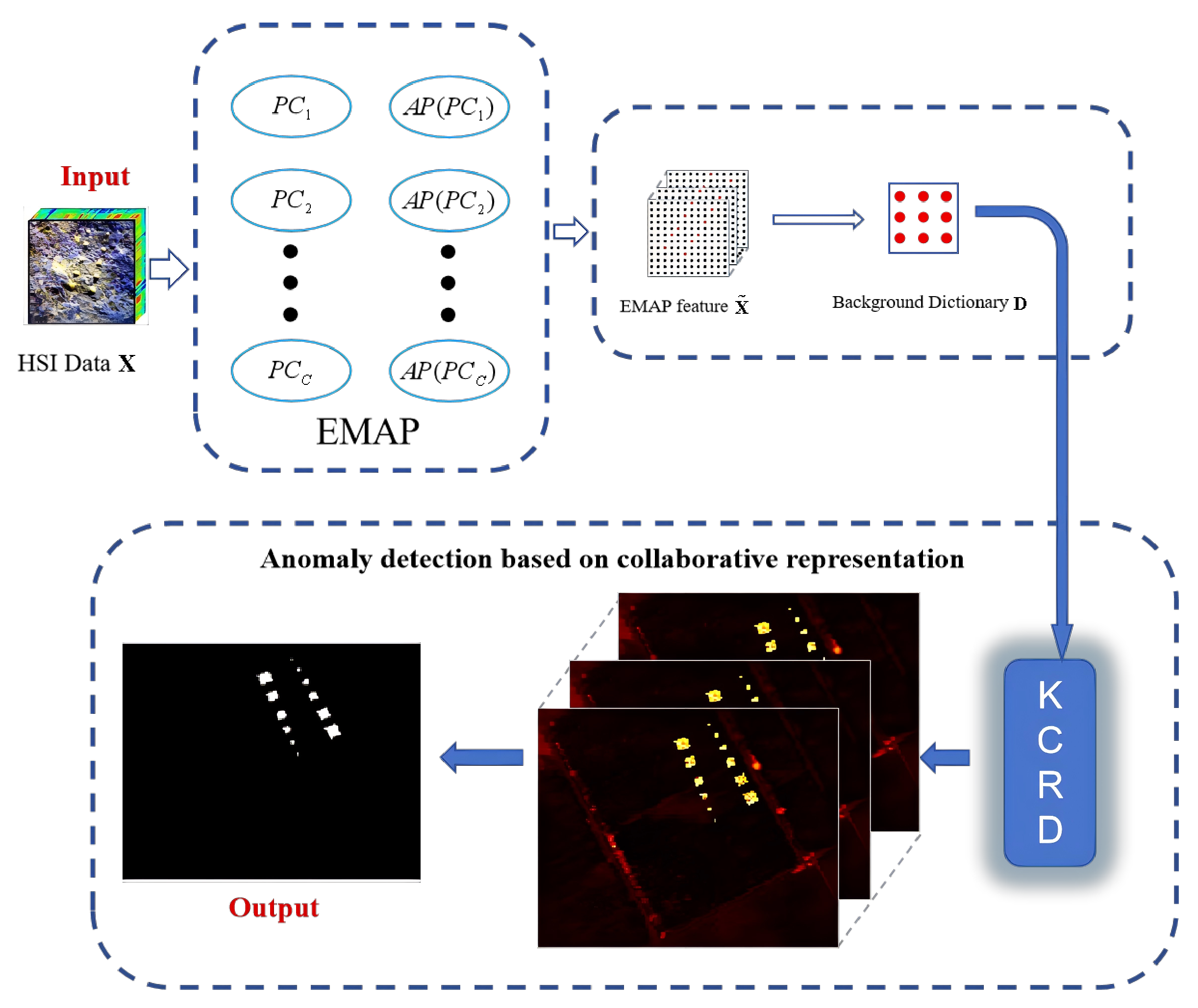
In this study, we introduce k-means CRD with extended multi-attribute profiles for hyperspectral anomaly detection (EMAPKCRD). Initially, the EMAP algorithm is employed to extract spatial information from hyperspectral images. Diverging from conventional CRD algorithms, our approach utilizes the k-means clustering algorithm to segregate anomalous pixels with similar characteristics and derive a reconstructed background dictionary matrix. Subsequently, by using the reconstructed background matrix obtained from clustering as input for anomaly detection within the CRD algorithm. We achieve a significant reduction in the computational complexity associated with traditional CRD algorithms. The detailed process is illustrated in Figure 2.

3.1. Extended Multi-Attribute Profiles

Morphological attribute profiles (AP) [38] enable the execution of specific operations based on predefined morphological properties. This process leads to the generation of a collection of refined attribute profiles and coarsened attribute profiles, which are subsequently combined in a single visual representation. The Extended Multi-Form Attribute Profile (EMAP) [39] method is a comprehensive approach that integrates and layers various contour feature maps derived from the AP algorithm. To analyze the single-band image f , we first apply a coarsening process on its attributes and then utilize sparsity techniques to compute the accuracy performance metric (AP). By evaluating the subject against every component within the dataset, a comprehensive collection of characteristics is derived.
A P ( f ) = { φ 1 ( f ) , , φ n ( f ) , f , γ 1 ( f ) , , γ n ( f ) } .
In order to reduce the complexity of hyperspectral image processing, principal component analysis is usually used to perform dimensionality reduction on the images. We assume that the number of channels after dimensionality reduction is c , and the extended morphological attribute profile (EAP) is the stacked feature map obtained by AP operation on the single band image of each channel.
E A P = { A P ( P C 1 ) , A P ( P C 2 ) , , A P ( P C c ) } .
where P C i represents the i-th principal component. By overlaying multiple morphological attribute profiles, we can obtain multi-morphological attribute profiles.
EMAP = { EAP a 1 , EAP a 2 , , EAP a n } .
where a i represents the i-th morphological attribute.
The commonly used morphological attributes include area, diagonal length of the outer moment of area, moment of inertia, standard deviation, etc. EMAP has a stronger ability to extract spatial features and has advantages in extracting the spatial structure of images.
In this study, for the input hyperspectral image, we first apply principal component analysis to obtain C principal component images. Then, using morphological filtering, we employ morphological attribute filters to generate morphological attribute EAPs on each principal component image. The EAPs are further extended to multi-attribute profiles (EMAPs), which include four different attributes: region area, region size, region elongation, and region homogeneity. Finally, all EAPs derived from different attributes are concatenated to form the EMAP features. The matrix representation of EMAP features is x ˜ R n × d 4 , where d 4 is related to the attribute filter parameters and the number of principal components. According to [38], each attribute can generate nine features. If we use an image with c  = 3, then d 4  = 9 × 4 × 3 = 108. The process of generating EMAP features can be summarized in Algorithm 1.
Algorithm 1 EMAP
Input: 
Hyperspectral data x ˜ R n × d , the number of principal components c.
  • Calculate its AP by Equation (8).
  • After performing AP operations on the single band images of each channel, the Extended Morphological Attribute Profile (EAP) is obtained by Equation (9).
  • Stacking multiple EAP features together to obtain EMAP features by Equation (10).
Output: 
EMAP feature matrix x ˜ R n × d 4 , where d 4 = 9 × 4 × c .

3.2. Window Reconstruction Model Based on K-Means Clustering

The CRD algorithm adopts a sliding dual window strategy in background reconstruction, which not only has high computational cost, but also requires resetting the window size every time the dataset changes, making it difficult to widely apply. The ERCRD algorithm uses a random selection strategy in background reconstruction, which saves computational power, but the selected points are not representative. When reconstructing the background, it cannot obtain an ideal dictionary matrix, which affects the accuracy of detection.
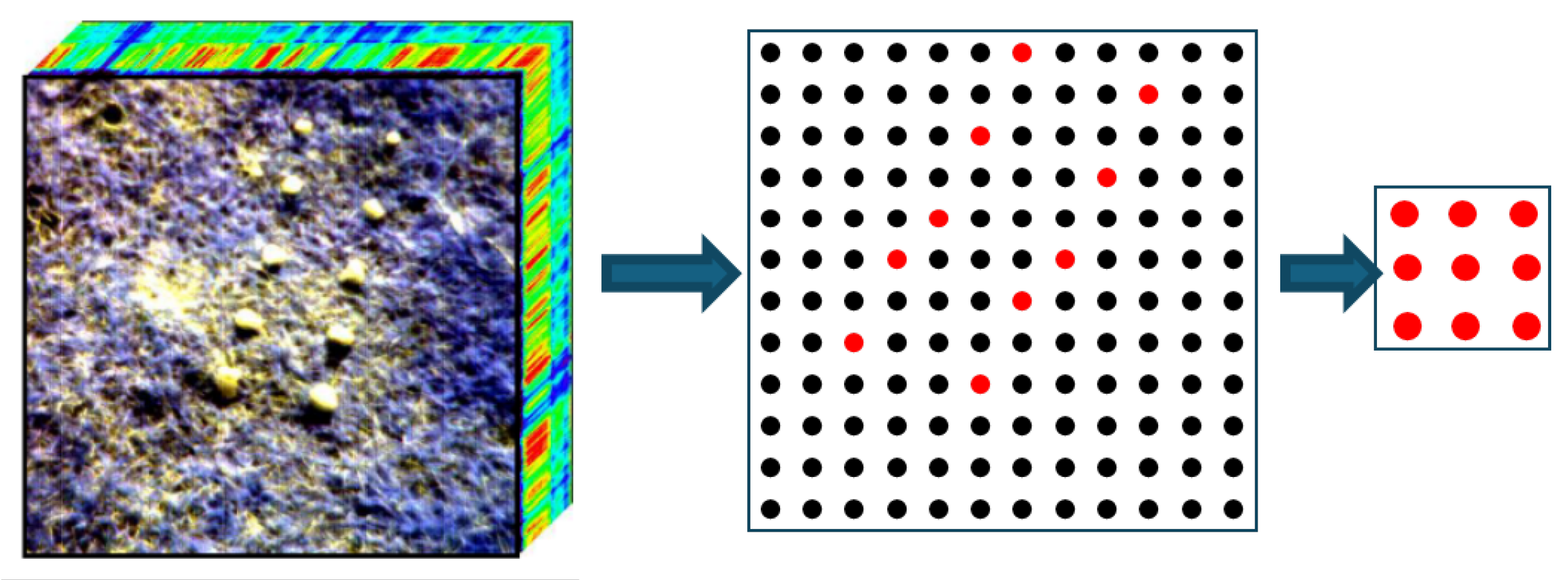
As shown in Figure 3, red indicates the position of abnormal pixel points in this paper we use k-means clustering to select representative points in the image for window reconstruction, which can effectively solve the problems of large computational complexity and non representativeness of the background dictionary caused by traditional CRD algorithm and improved ERCRD algorithm in window reconstruction.
For hyperspectral images, given a feature matrix X ˜ = x 1 , x 2 , x 3 , x n obtained by EMAP, record x ˜ R n × d 4 as the data matrix, where x i R d 4 × 1 is the pixel point.
Randomly select k center points to form the background dictionary matrix D R k × d 4
D = x 1 , x 2 , x 3 , x k .
For each pixel x i , calculate its distance from the center point x j . Pixel x i belongs to cluster c ( j ) of the center point x j that is closest to it.
c ( j ) = arg min x i x j 2 , i 1 , 2 , d 4 , j 1 , 2 , k .
For each obtained cluster c ( j ) , recalculate the position of the center point
x j = i = 1 d 4 l c ( i ) = j x i i = 1 d 4 l c ( i ) = j .
Continuously update the position of the center point until δ j is less than a certain threshold ε and stop
δ j = x j m + 1 x j m 2 .
where x j m + 1 is the result of the m + 1 th calculation, and  x j m is the result of the mth calculation.
Then, we will obtain dictionary matrix D
D = x 1 , x 2 , x 3 , x k .
The process of generating the reconstructed background matrix D is indicated in Algorithm 2.
Algorithm 2 K-means Clustering
Input: 
EMAP feature matrix X ˜ , number of clusters k .
  • Randomly select k points to generate a background dictionary matrix D .
  • Calculate the cluster c ( j ) where pixel x i belongs to the point x j closest to it.
  • Update the position of the center point and stop when δ j = x j m + 1 x j m 2 is less than a certain threshold.
Output: 
Output a new background dictionary matrix D .

3.3. EMAPKCRD

Constructing the objective function based on the idea of collaborative representation
min a X ˜ Da 2 2 + λ a 2 2
where D R k × n is the reconstructed dictionary matrix obtained through k-means clustering, and  λ is the regularization parameter.
Similarly, Tikhonov regularization Γ y with distance weights is introduced to adjust the value of weight vector a , and the objective function can be rewritten as
min a X ˜ Da 2 2 + λ Γ y a 2 2
To make the algorithm more stable, we add a constraint of coefficient 1 to the weight vector a . At this point, the objective function is modified to
min a X ^ Da ^ 2 2 + λ Γ y a 2 2
where x ^ = x ; 1 , D ^ = D ; 1 . Our goal is to find a weight vector a that minimizes x ^ D ^ a 2 2 while satisfying the constraint of minimizing a 2 2 . By taking the derivative of a in the above equation, we obtain
a = D ^ T D ^ + λ Γ y T Γ y 1 D ^ T x ^
Reconstruct pixels and calculate reconstruction errors
δ = X ˜ D a 2 2
The EMAPKCRD process can be summarized in Algorithm 3.
Algorithm 3 EMAPKCRD
Input: 
Hyperspectral dataset X , main component count c , number of clusters k .
  • Extract EMAP features and obtain feature matrix X ˜ .
  • Use k-means clustering algorithm to obtain reconstructed background dictionary matrix D .
  • Obtain abnormal scores through CRD algorithm.
Output: 
Abnormal scores for all pixels.

4. Experiments and Results

In this section, we perform a comprehensive evaluation of our proposed detection method by analyzing four real-world hyperspectral datasets and one synthetic dataset, all of which are utilized to assess the effectiveness of our approach.The study utilized MATLAB 2024a as the primary computational platform, executed on a high-performance computing system equipped with an Intel i7-9700K processor operating at a clock speed of 3.60 GHz. Here are the comprehensive details:
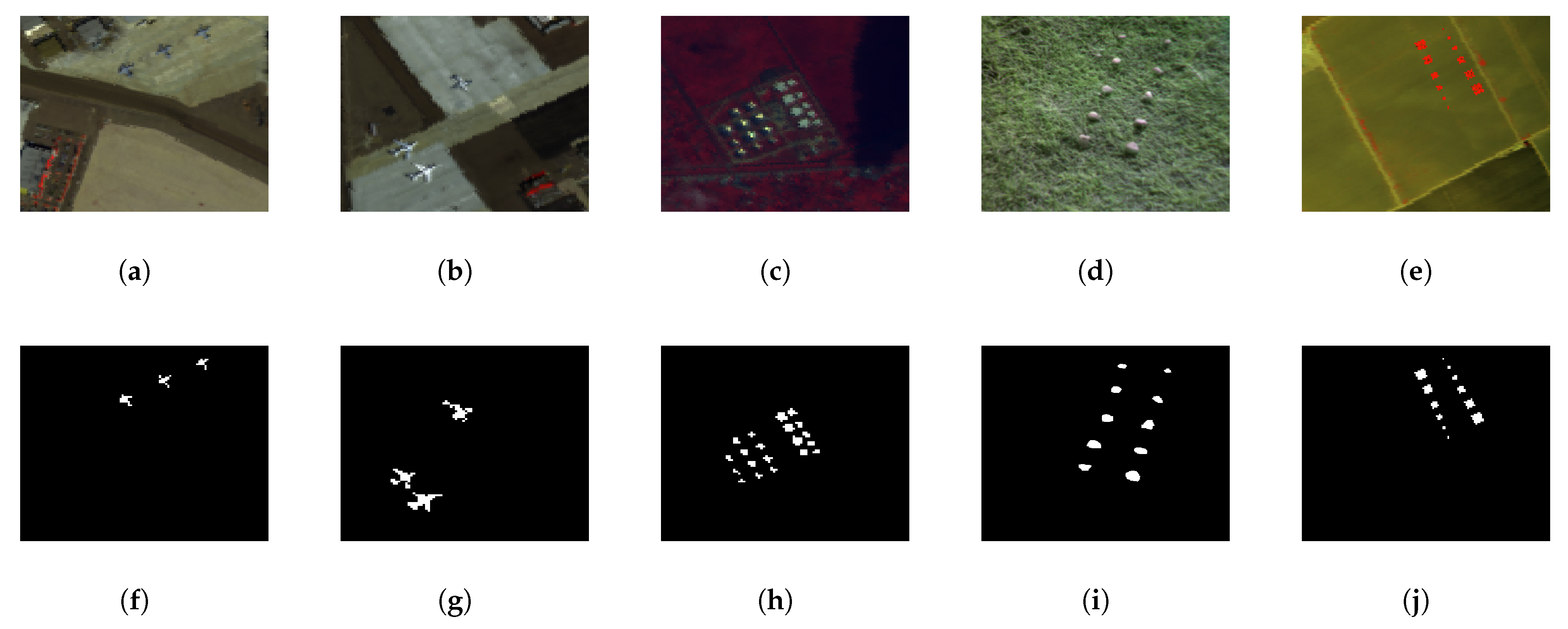
  • AVIRIS-I dataset: As depicted in the accompanying figure, it provides a comprehensive visual representation of the spectral reflectance properties of the agricultural field under study. In the case of (a) and (f), the data was collected using the Airborne Visible/Infrared Imaging Spectrometer (AVIRIS) instrument stationed at the San Diego, California, USA facility. The visual representation of the scene spans a resolution of 400 pixels in both width and height, and is composed of 224 distinct spectral bands, each corresponding to a unique wavelength range that stretches from 370 nanometers to 2510 nanometers. As referenced in [7], the AVIRIS-I dataset occupies a specific region within the image, located at the upper-left quadrant, and spans 120 pixels by 120 pixels. Following the elimination of bands associated with water absorption, reduced signal-to-noise ratios, and suboptimal quality, a total of 189 distinct spectral components were retained during the experimental analysis. In this region, a cluster of three distinct planes each containing 58 pixels appears to be associated with anomalous data points.
  • AVIRIS-II dataset: As shown in Figure 4b,g, this dataset was also obtained from San Diego with a pixel size of 100 × 100. According to [40], in this image, the abnormal pixels are three planes composed of 138 pixels.
  • abu-urban-2 dataset: The Abu-urban-2 dataset is a high-resolution urban landscape map derived from the ABU collection, comprising 210 spectral bands. This instrument operates across a broad spectral range, spanning from 400 nanometers to 2500 nanometers, and achieves a resolution of 10 nanometers in terms of wavelength. The Abu-urban-2 dataset is composed of a 100 × 100 pixel resolution and spans a total of 207 distinct spectral bands, which are used for multispectral analysis. According to [40] various vehicles in the map are considered abnormal pixels and should be detected. The false color image and ground truth image of the abu-urban-2 dataset are shown in Figure 4c and Figure 4h, respectively.
  • Cri dataset: This dataset was obtained from the Nuance Cri hyperspectral sensor and obtained from [7]. It has a size of 400 × 400 pixels and contains 46 spectral bands with a wavelength range of 650 to 1100 nm. In this image, rocks composed of 2216 pixels were identified as abnormal pixels and should be detected. The false color map and ground truth map of this dataset are shown in the Figure 4d,i.
  • Salinas simulation dataset [11]: This dataset is a simulated dataset. Firstly, a binary mask image M with pixel sizes of 150 and 126 is constructed by generating six square matrices. Then, a region I of the same size as the binary mask image M cut out from the Salinas scene datatset is used to construct the synthesized image I . In this image, 12 blocks with side lengths ranging from 1 to 6 pixels in opposite order are considered abnormal.
    I i , j = M i , j · ϕ k + 1 M i , j · I i , j .
    Based on the real images of the Salinas scene scene, setting the parameter k to 14, the final simulated dataset’s false color image and ground truth image are shown in Figure 4e,j.

4.1. Evaluation Methods

In this experiment, false color images are employed as a qualitative measure for evaluating detection outcomes. Additionally, the receiver operating characteristic (ROC) curve and area under the curve (AUC) [41] are utilized to quantitatively assess the performance of the anomaly detection algorithms. The core of the ROC curve lies in continuously traversing all possible thresholds, calculating the “False Positive Rate (FPR)” and “True Positive Rate (TPR)” corresponding to each threshold, and then connecting these (FPR, TPR) coordinate points to form the curve. In the ROC coordinate graph, a curve that approaches the upper left corner signifies a larger AUC value, which indicates superior detection performance.
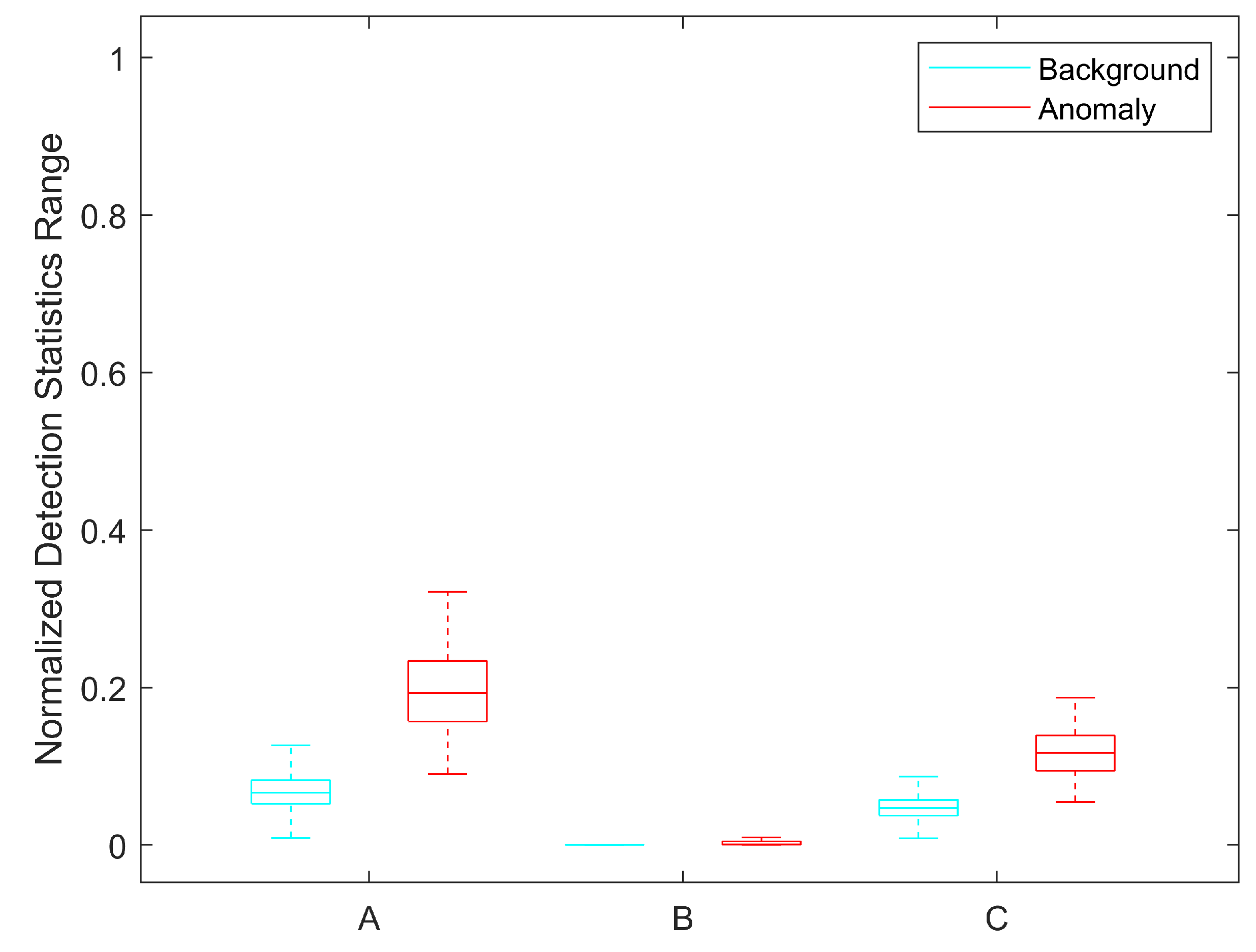
To more intuitively illustrate the degree of separation between anomalies and background, box plots are employed to assess the performance of anomaly detection algorithms. When generating the box plot, we use the ground truth labels (gt) to separate the detection scores of background and anomalies. As depicted in Figure 5, the red color denotes the distribution of abnormal pixels, while blue represents the distribution of background pixels. A larger interval among the red and blue distributions signifies greater separation between background and abnormal pixels. A shorter blue box indicates a more effective suppression of the background by the algorithm. Consequently, this separation visualization provides a more intuitive demonstration of the algorithm’s detection performance. As illustrated in Figure 5, detector B exhibits the best performance in background suppression, whereas detector A excels in separating anomalies from the background.

4.2. Compared Methods

To indicate the effects of the EMAPKCRD method, we conducted a comparative analysis with classical algorithms, current advanced algorithms, and variants of the CRD algorithm in the experiment.
  • GRX: Global RX detector. This algorithm models the background using the entire image. Although the method is simple and efficient, it only produces good results for some images with relatively simple topological structures.
  • LRX: Local RX algorithm, using a dual window model to capture local areas for modeling, can protect background pixels from interference when testing abnormal pixels. However, the choice of window size has brought poor robustness to LRX.
  • CBAD: Clustering-based anomaly detection algorithm. This method clusters background pixels and then uses the RX method for anomaly detection, which can obtain satisfying results, but lacks consideration for the weight of each category.
  • LSMAD: Low rank and sparse matrix factorization-based anomaly detection. This method uses the background part after data decomposition to estimate the background, and then performs RX anomaly detection. It can improve the robustness of the algorithm.
  • CRD: Collaborative Representation based Anomaly Detection (CRD) Algorithm. This method assumes that each background pixel can be approximately represented linearly by its surrounding pixels. However, due to its sliding dual window strategy, the algorithm has a high complexity and longer detection time in actual detection.
  • RCRD: A hyperspectral image anomaly detector based on fast recursive collaborative representation. This method constructs two elementary transformation matrices based on the position of pixels, and uses matrix inversion lemma to derive a recursive update method to improve the detection speed of the detector.

4.3. Detection Result

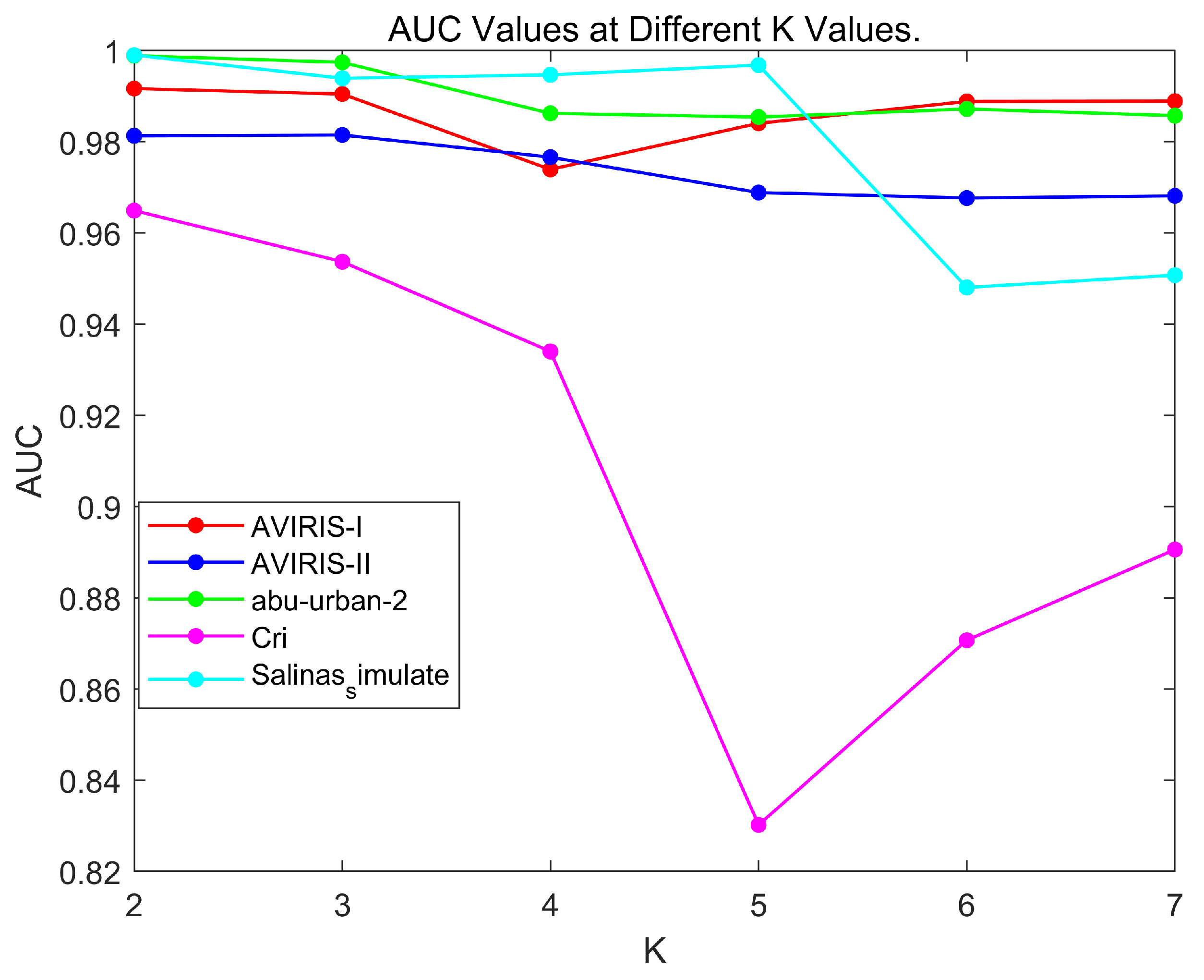
Then, we conduct experiments on the five datasets mentioned above to verify the effectiveness of our method. Before the experiment began, to determine the selection of parameter k, we tested the anomaly detection AUC values under different k values on five data sets. It can be seen directly from Figure 6 that the experimental results are best when k equals 2. Therefore, for the EMAPKCRD method, we set the number of principal components c = 5, selected k = 2 for clustering during window reconstruction. For the CRD algorithm, the inner window size is 13, and the outer window size is 17. The regularization parameter λ for all three methods was set to 10 6 . The experimental results on each dataset are as follows:
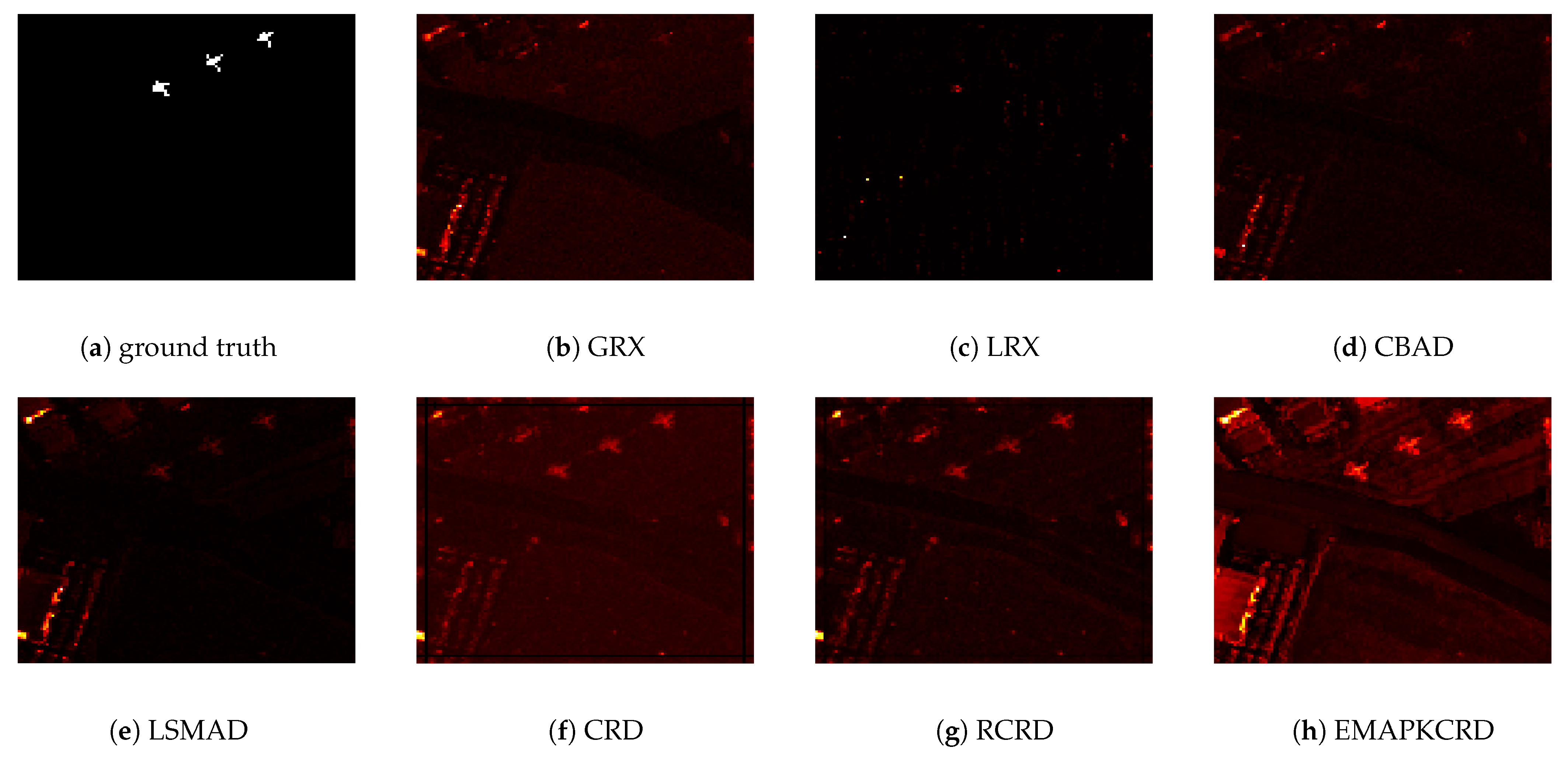
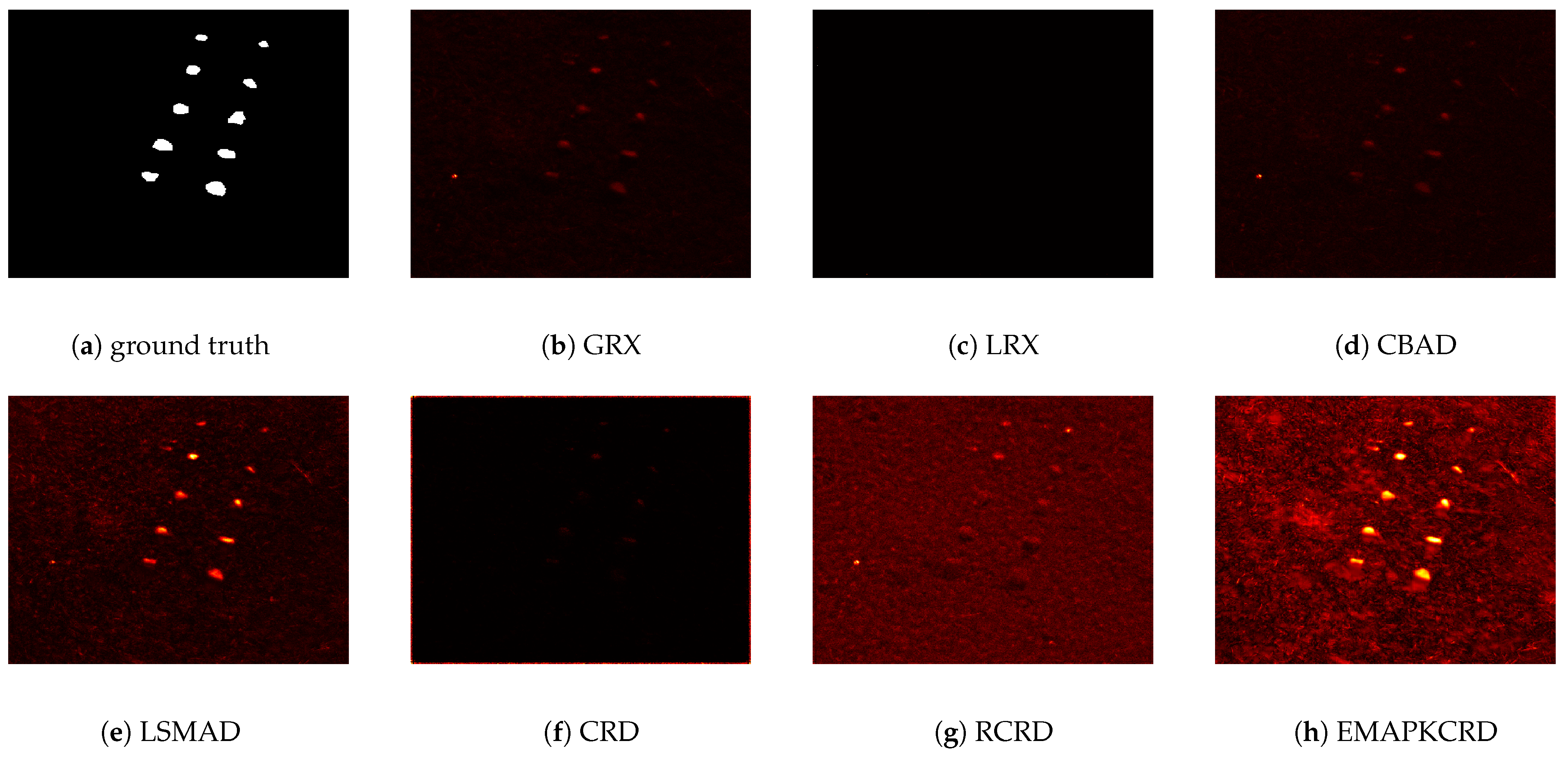
As illustrated in Figure 7, the EMAPKCRD method proposed in this study can not only detect the positions of three aircraft with high precision in the AVIRIS-I dataset (a hyperspectral dataset acquired by the Airborne Visible/Infrared Imaging Spectrometer (AVIRIS) over the San Diego area, California, USA) but also effectively delineate the contour shapes of the aircraft. In contrast, the LRX (Local RX) algorithm has limited capability in locating anomalous pixels; meanwhile, other anomaly detection algorithms such as GRX (Global RX), CBAD (Clustering-Based Anomaly Detection), and LSMAD (Low-Rank and Sparse Matrix Factorization-Based Anomaly Detection) fail to detect anomalous targets clearly. Figure 8 presents the experimentally obtained Receiver Operating Characteristic (ROC) curve, the corresponding Area Under the Curve (AUC) value, and the normalized anomaly–background separation map. The results show that, compared with the ROC curves of other algorithms, the ROC curve of the EMAPKCRD anomaly detection algorithm proposed in this study is closer to the upper-left corner of the coordinate plane. The AUC value achieved by this method is 0.9916—although the gap between this value and those of other comparative algorithms is relatively small, it is still higher than all other methods in the experiment. Moreover, from the anomaly–background separation map and Figure 6, it can be seen that the proposed method can better highlight the positions and shapes of anomalous targets and achieves the best separation effect between anomalous targets and background pixels.
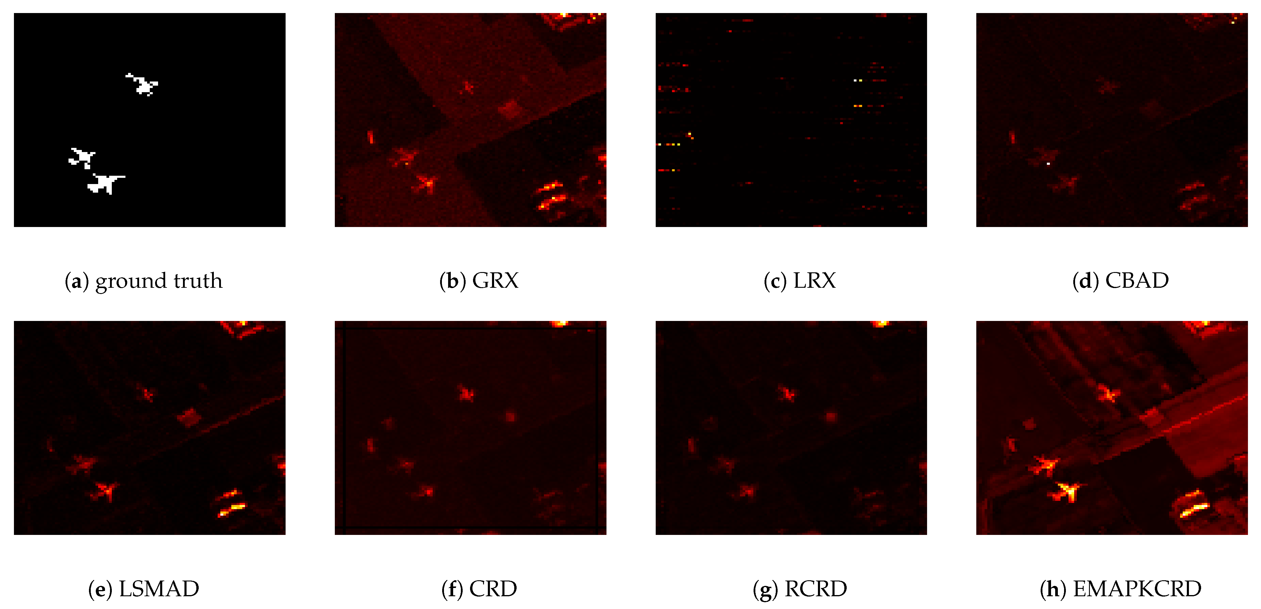
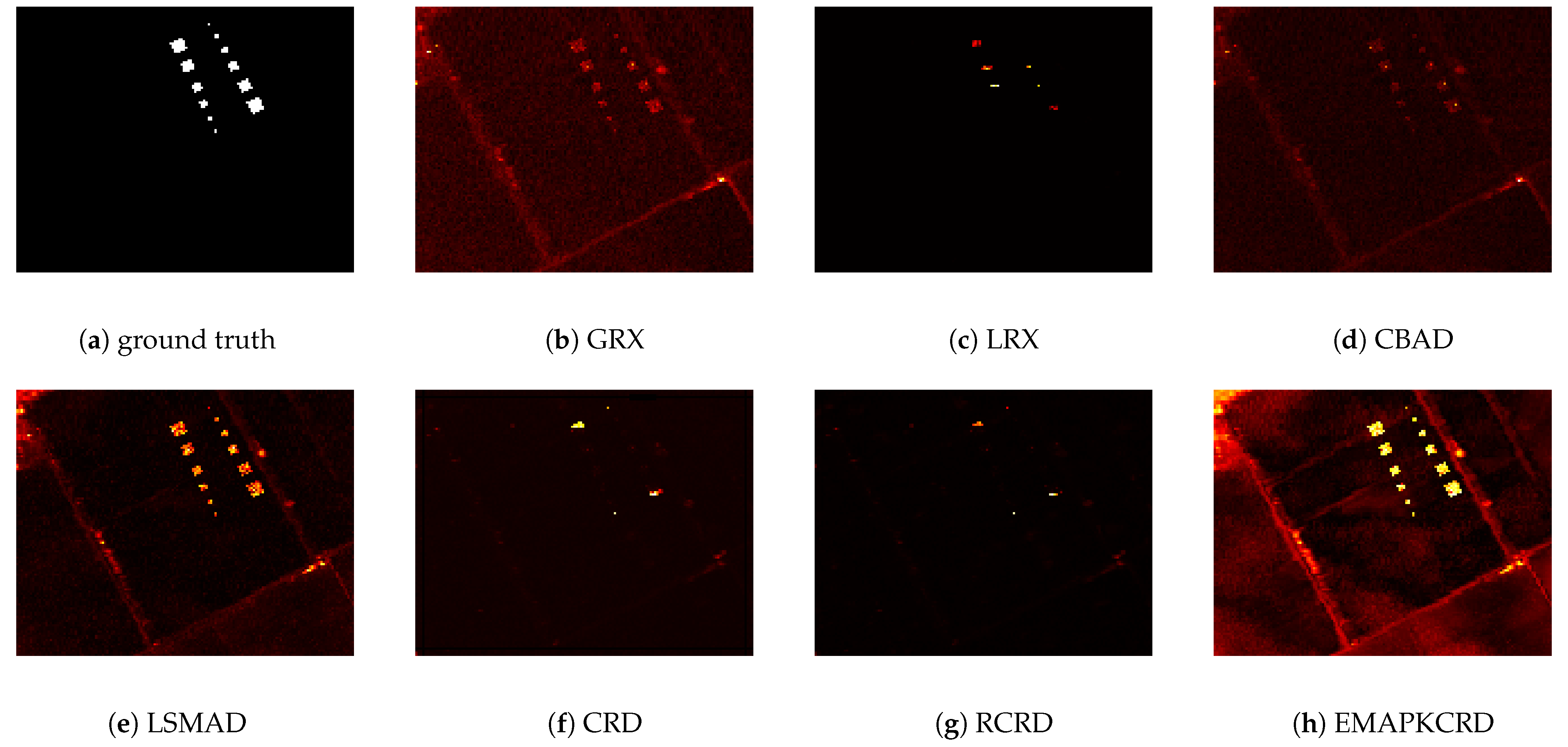
The detection outcomes of various methods applied to the AVIRIS-II dataset are illustrated in Figure 9. The EMAPKCRD method introduced in this study demonstrates highest accuracy in identifying the positions and profiles of three aircraft. In contrast, the LRX detector fails to pinpoint the anomaly’s location. The GRX, CBAD, LSMAD, and RCRD detectors are capable of generally identifying the anomaly’s location; however, their results lack clarity. The CRD detector successfully delineates the outlines of two aircraft, but the third aircraft is not distinctly visible, and the CRD method erroneously classifies some background pixels as anomalies. In Figure 10, the experiment yielded the ROC curve, the corresponding AUC value, and the normalized background anomaly separation graph. The ROC curve for the EMAPKCRD anomaly detection algorithm proposed in this paper is positioned closer to the upper left corner of the coordinate plane compared to the curves of other algorithms. The AUC value for the EMAPKCRD method is 0.9813, surpassing those of other methods. The normalized background anomaly separation graph further indicates the superior performance of the proposed method in the extraction of anomaly targets.
In the context of the abu-urban-2 dataset, the detection outcomes of various methodologies are illustrated in Figure 11. The EMAPKCRD method, as introduced in this study, demonstrates a clear capability to identify all anomalous points. In contrast, the CBAD method fails to distinguish between background and anomalies, erroneously classifying the majority of background pixels as anomalies. The anomaly detectors LRX, CRD, RCRD, and LSMAD are limited to identifying only a subset of outlier pixels, which results in suboptimal detection performance. Although the GRX method is capable of identifying all anomalous pixels, its clarity is inferior compared to that of EMAPKCRD. Figure 12 presents the ROC curve, associated AUC values, and the normalized background anomaly separation plot. It is evident from the figure that the ROC curve for the EMAPKCRD anomaly detection algorithm is positioned closer to the upper left corner of the coordinate plane than those of the other algorithms. The AUC value of the EMAPKCRD method is 0.9989, which is higher than all other methods in the experiment. Furthermore, the normalized background anomaly separation map and the color detection map indicate that the EMAPKCRD anomaly detector not only effectively detects anomalous pixels but also achieves superior separation of anomalies from the background, thereby facilitating the identification of anomalous pixels.
In the analysis of the Cri dataset, the detection outcomes of various methods are illustrated in Figure 13. The EMAPKCRD method, introduced in this study, demonstrates superior capability in distinctly identifying pixels deemed abnormal within the image. In contrast, the LRX and CRD methods exhibit limited ability to discern between background and anomalies, while CBAD, GRX, and RCRD methods only vaguely identify the locations of anomalous pixels. However, these methods show low differentiation between background and anomalous pixels, making it difficult to clearly discern the anomalies’ locations. Figure 14 reveals that both the LSMAD and the EMAPKCRD algorithms effectively pinpoint the locations of abnormal pixels. Nonetheless, the ROC curve and AUC value indicate that the proposed method achieves a position closer to the upper left corner of the coordinate plane compared to other algorithms. From the perspective of anomaly–background separation, the method proposed in this study exhibits the most effective anomaly separation performance.
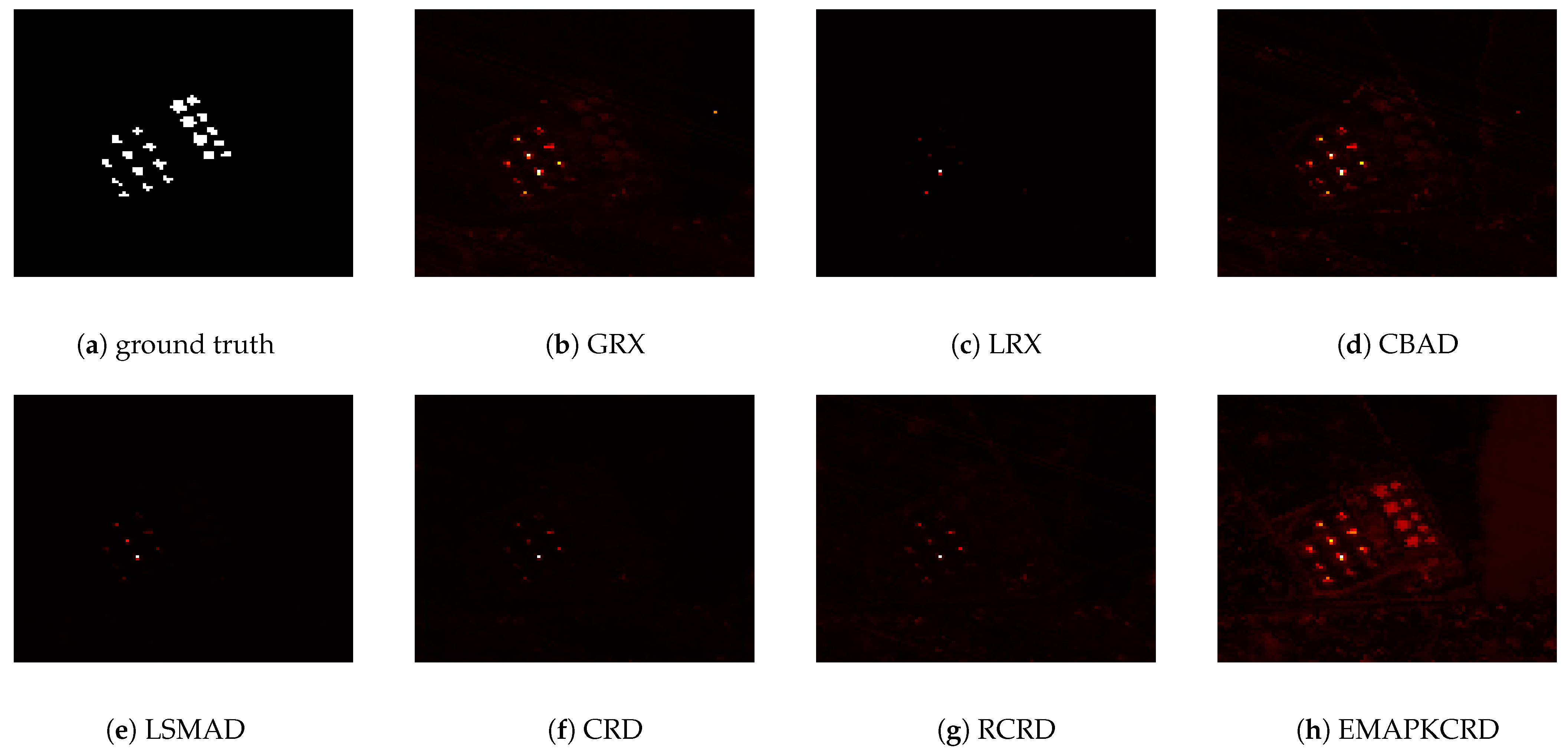
In the context of the Salinas simulation dataset, Figure 15 illustrates the detection outcomes of various methodologies. The EMAPKCRD method, introduced in this study, demonstrates a clear capability to identify all anomalous pixels. In contrast, the LRX, CRD, and RCRD anomaly detection algorithms exhibit a limited capacity to detect anomalies. While the GRX and CBAD algorithms can identify anomalies, they also erroneously classify certain background pixels as anomalies. The LSMAD method effectively detects the locations of all anomalies; however, the EMAPKCRD method offers superior separation between background and anomalies, thereby providing a clearer representation of anomalous pixels. Figure 16 presents the ROC curve, corresponding AUC values, and a normalized background anomaly separation plot. It is evident from the figure that the ROC curve for the EMAPKCRD anomaly detection algorithm is positioned closer to the upper left corner of the coordinate plane compared to the curves of other algorithms, indicating its enhanced performance. The EMAPKCRD method achieved an AUC value of 0.9990, which is higher than all other methods in the experiment. Analysis of the background anomaly separation and color detection graphs indicates that the EMAPKCRD anomaly detector excels in identifying abnormal pixels while effectively distinguishing anomalies from the background, thereby facilitating the identification process.
To further assess the efficacy of the proposed method in anomaly detection, we conduct a second phase of experimentation, evaluating its performance across five datasets. This evaluation primarily involved a comparative analysis of the time efficiency and AUC values between the CRD algorithm and its variant, RCRD. The results, presented in the accompanying Table 1 and Table 2, demonstrate that the proposed method significantly outperforms the previous CRD algorithm and its variants in both AUC values and detection time, thereby substantiating the enhanced effectiveness of the constructed approach.

5. Discussion

In this paper, we propose a fast collaborative representation algorithm based on Extended Multi-Attribute Profiles for HAD. Comparative experimental results demonstrate that our proposed method achieves excellent performance both in terms of detection accuracy and the effectiveness of anomaly–background separation. Specifically, on the abu-urban-2 dataset, compared with the traditional CRD [33] method and the improved Recursive Collaborative Representation Detector (RCRD) [34] method, our method increases the AUC by 6.8 % and 18 % , respectively. In terms of detection speed, the proposed method takes only 0.12 and 0.14 times the time consumed by CRD and RCRD, respectively. This result benefits from two key improvements: first, the integration of EMAP, which fully exploits spatial features—this is crucial for enhancing detection accuracy; second, the optimization of background dictionary construction using the k-means clustering algorithm. By employing k-means clustering to select representative background pixels, we reduce the interference of anomalous pixels in background modeling, and the dimension of the dictionary is reduced from N to k, leading to an exponential decrease in computational complexity. Through validation, the method proposed in this paper meets the requirements of high accuracy and real-time performance.
However, this method still has certain limitations. Firstly, it exhibits dependence on dataset characteristics: when processing datasets with different spectral features, spatial resolutions, noise levels, or anomalous target features, the effectiveness and stability of the method may be affected, and its generalization ability needs further verification. Secondly, on some datasets, the performance gap between our method and other algorithms is relatively small, so it may not meet the application requirements in scenarios requiring extremely high detection accuracy. In future research, intelligent methods can be attempted to further improve detection accuracy to adapt to the needs of military application scenarios.

6. Conclusions

In this study, we introduce a novel clustering algorithm based on k-means that integrates extended multi-attribute profiles for hyperspectral anomaly detection (EMAPKCRD). At the outset, we utilize the extended multi-attribute profile (EMAP) method to derive spatial characteristics from hyperspectral data. By effectively integrating the spatial characteristics of hyperspectral imagery (HSI), we are able to significantly improve the detection accuracy and reliability of our system. Subsequently, for the extracted feature images, we apply the k-means clustering algorithm to select representative points for window reconstruction, followed by anomaly detection based on the concept of collaborative representation. By fully exploiting the spatial features of hyperspectral images and purifying the background, this method meets the requirements of both high accuracy and real-time performance. In the experimental section, we first compare six methods across five datasets. The experimental results demonstrate that the EMAPKCRD method consistently achieves the highest AUC for anomaly detection when compared to other methods. Additionally, we compare detection time and performance with CRD variants across the same five datasets. The results indicate that, relative to the traditional CRD algorithm, the method proposed in this paper achieves higher detection accuracy in a shorter time frame. The superiority of the EMAPKCRD method is thus empirically validated.

Author Contributions

Validation, F.H. and S.F.; Writing—original draft, F.H. and S.F.; Writing—review & editing, F.H., S.F., J.Z. and J.D.; Supervision, H.H.,W.J. and J.Z. All authors have read and agreed to the published version of the manuscript.

Funding

This research was sponsored by the National Natural Science Foundation of China (Grant No. 62001500, 42301458, 42401499, and 12403080), in part Supported by the China Postdoctoral Science Foundation under Grant Number 2025T181182, 2023M734288, and 2023M744301, in part Supported by the National Social Science Fund under Grant Number 2023-SKJJ-C-028, in part supported by Shaanxi Province Support Fund under Grant Number 20230712.

Data Availability Statement

The original contributions presented in this study are included in the article. Further inquiries can be directed to the corresponding author.

Conflicts of Interest

The authors declare no conflicts of interest.

References

  1. Shen, X.; Bao, W.; Liang, H.; Zhang, X.; Ma, X. Grouped Collaborative Representation for Hyperspectral Image Classification Using a Two-Phase Strategy. IEEE Geosci. Remote Sens. Lett. 2022, 19, 1–5. [Google Scholar] [CrossRef]
  2. Dong, S.; Feng, W.; Long, Y.; Bao, W.; Li, K.; Dauphin, G.; Quan, Y. Hyperspectral Image Classification Method Based on Data Expansion and Consistency Regularization with Small Samples. IEEE Geosci. Remote Sens. Lett. 2025, 22, 1–5. [Google Scholar] [CrossRef]
  3. Li, S.; Zhang, K.; Duan, P.; Kang, X. Hyperspectral Anomaly Detection with Kernel Isolation Forest. IEEE Trans. Geosci. Remote. Sens. 2020, 58, 319–329. [Google Scholar] [CrossRef]
  4. Patel, N.K.; Patnaik, C.; Dutta, S.; Shekh, A.M.; Dave, A.J. Study of crop growth parameters using Airborne Imaging Spectrometer data. Int. J. Remote Sens. 2001, 22, 2401–2411. [Google Scholar] [CrossRef]
  5. Shaw, G.; Manolakis, D. Signal processing for hyperspectral image exploitation. IEEE Signal Process. Mag. 2002, 19, 12–16. [Google Scholar] [CrossRef]
  6. Du, B.; Zhang, L. Random-Selection-Based Anomaly Detector for Hyperspectral Imagery. IEEE Trans. Geosci. Remote Sens. 2011, 49, 1578–1589. [Google Scholar] [CrossRef]
  7. Xu, Y.; Wu, Z.; Li, J.; Plaza, A.; Wei, Z. Anomaly Detection in Hyperspectral Images Based on Low-Rank and Sparse Representation. IEEE Trans. Geosci. Remote Sens. 2016, 54, 1990–2000. [Google Scholar] [CrossRef]
  8. Huyan, N.; Zhang, X.; Zhou, H. Hyperspectral Anomaly Detection via Background and Potential Anomaly Dictionaries Construction. IEEE Trans. Geosci. Remote Sens. 2019, 57, 2263–2276. [Google Scholar] [CrossRef]
  9. Cai, W.; Ning, X.; Zhou, G.; Bai, X.; Jiang, Y.; Li, W.; Qian, P. A Novel Hyperspectral Image Classification Model Using Bole Convolution with Three-Directions Attention Mechanism: Small sample and Unbalanced Learning. IEEE Trans. Geosci. Remote. Sens. 2022, 61, 5500917. [Google Scholar] [CrossRef]
  10. Cai, W.; Wei, Z. Remote Sensing Image Classification Based on a Cross-Attention Mechanism and Graph Convolution. IEEE Geosci. Remote Sens. Lett. 2022, 19, 1–5. [Google Scholar] [CrossRef]
  11. He, F.; Yan, S.; Ding, Y.; Sun, Z.; Zhao, J.; Hu, H.; Zhu, Y. Recursive RX with Extended Multi-Attribute Profiles for Hyperspectral Anomaly Detection. Remote Sens. 2023, 15, 589. [Google Scholar] [CrossRef]
  12. Chu, Y.; Wang, Z.; Peng, J.; Ding, W.; Cao, H. Fuzzy Triple Contrastive Learning for Hyperspectral Image Classification. IEEE Trans. Geosci. Remote Sens. 2025, 63, 1–17. [Google Scholar] [CrossRef]
  13. Cao, Z.; Chen, S.; Li, J. Enhancing Hyperspectral Image Classification in Small Sample Settings Using Conditional Denoising Diffusion Implicit Model. IEEE Signal Process. Lett. 2025, 32, 2479–2483. [Google Scholar] [CrossRef]
  14. Wei, Y.; Niu, C.; Wang, H.; Liu, D. The Hyperspectral Image Clustering Based on Spatial Information and Spectral Clustering. In Proceedings of the 2019 IEEE 4th International Conference on Signal and Image Processing (ICSIP), Wuxi, China, 19–21 July 2019; pp. 127–131. [Google Scholar]
  15. Mei, Z.; Yin, Z. Self-Supervised Learning of Discriminative Spatial–Spectral Features for Hyperspectral Images Clustering. IEEE Geosci. Remote Sens. Lett. 2022, 19, 1–5. [Google Scholar] [CrossRef]
  16. Chi, J.; Shen, X.; Yu, H.; Shang, X.; Chanussot, J.; Shi, Y. Robust Linear Unmixing for Hyperspectral Remote Sensing Imagery Based on Enhanced Constraint of Classification. In Proceedings of the IGARSS 2022—2022 IEEE International Geoscience and Remote Sensing Symposium, Kuala Lumpur, Malaysia, 17–22 July 2022; pp. 1628–1631. [Google Scholar]
  17. Chen, J.; Li, J.; Gamba, P. A Multi-Tasks Autoencoder Hyperspectral Unmixing Model with Information Gain Based On Graph Network. In Proceedings of the Workshop on Hyperspectral Imaging and Signal Processing: Evolution in Remote Sensing (WHISPERS), Athens, Greece, 31 October–2 November 2023; pp. 1–5. [Google Scholar]
  18. Xiao, Z. Hyperspectral Image Denoising Based on Low-Rank Matrix Decomposition Image Prior. In Proceedings of the 2024 6th International Conference on Electronics and Communication, Network and Computer Technology (ECNCT), Guangzhou, China, 19–21 July 2024; pp. 56–59. [Google Scholar]
  19. Lin, P.; Jiang, X.; Sun, L. Hyperspectral Image Denoising Via Cosine Transform-Based Tensor Subspace Representation. In Proceedings of the 2023 13th Workshop on Hyperspectral Imaging and Signal Processing: Evolution in Remote Sensing, Athens, Greece, 31 October–2 November 2023; pp. 1–5. [Google Scholar]
  20. Ma, H.; Wang, Y.; Jiang, L.; Song, M.; Yu, C.; Zhao, E. Multi-Scale Fusion Maximum Entropy Subspace Clustering for Hyperspectral Band Selection. In Proceedings of the IEEE International Geoscience and Remote Sensing Symposium, Kuala Lumpur, Malaysia, 17–22 July 2022; pp. 779–782. [Google Scholar]
  21. Francis, J.; Shanthini, K.S.; George, S.N.; George, S. A Tensor Non-Convex Low Rank and Sparse Constrained Band Selection Scheme for Clustering of Hyperspectral Paper Data. In Proceedings of the 2022 12th Workshop on Hyperspectral Imaging and Signal Processing: Evolution in Remote Sensing (WHISPERS), Rome, Italy, 13–16 September 2022; pp. 1–5. [Google Scholar]
  22. Liang, C.; Chen, Z. A Self-Supervised Hierarchical Clustering Network For Multiple Change Detection In Multitemporal Hyper-spectral Images. In Proceedings of the 2022 12th Workshop on Hyperspectral Imaging and Signal Processing: Evolution in Remote Sensing (WHISPERS), Rome, Italy, 13–16 September 2022; pp. 1–4. [Google Scholar]
  23. Shammi, S.A.; Du, Q. Hyperspectral Image Change Detection Using Deep Learning and Band Expansion. In Proceedings of the 2022 12th Workshop on Hyperspectral Imaging and Signal Processing: Evolution in Remote Sensing (WHISPERS), Rome, Italy, 13–16 September 2022; pp. 1–5. [Google Scholar]
  24. Han, X.; Wei, Y.; Zhang, H.; Xu, Q.; Sun, W. Tuning to Real for Single-Spectrum Hyperspectral Target Detection. In Proceedings of the 2023 13th Workshop on Hyperspectral Imaging and Signal Processing: Evolution in Remote Sensing (WHISPERS), Athens, Greece, 31 October–2 November 2023; pp. 1–5. [Google Scholar]
  25. Li, G.; Hao, H.; Wu, L.; Liu, B. Current Situation of Denoising And Target Detection In Hyperspectral Images. In Proceedings of the 2022 3rd International Conference on Geology, Mapping and Remote Sensing (ICGMRS), Zhoushan, China, 22–24 April 2022; pp. 555–559. [Google Scholar]
  26. Wang, Y.; Sun, J.; Xu, Y.; Wei, Z.; Zheng, S.; Wu, Z. Fast Processing of Massive Hyperspectral Image Anomaly Detection Based on Cloud-Edge Collaboration. IEEE J. Sel. Top. Appl. Earth Obs. Remote Sens. 2025, 18, 14644–14657. [Google Scholar] [CrossRef]
  27. Wang, Y.; Li, W.; Gui, Y.; Xie, H.; Zhang, L. A Generalized Non-Convex Surrogated Framework for Anomaly Detection on Blurred Hyperspectral Images. IEEE Trans. Image Process. 2025, 34, 3108–3122. [Google Scholar] [CrossRef] [PubMed]
  28. Wu, Z.; Tao, X.; Paoletti, M.E.; Haut, J.M.; Pastor-Vargas, R.; Plaza, A. Deep Unrolling Network with Active Dictionary Learning for Hyperspectral Anomaly Detection. In Proceedings of the 2023 13th Workshop on Hyperspectral Imaging and Signal Processing: Evolution in Remote Sensing (WHISPERS), Athens, Greece, 31 October–2 November 2023; pp. 1–5. [Google Scholar]
  29. Reed, I.S.; Yu, X. Adaptive multiple-band CFAR detection of an optical pattern with unknown spectral distribution. IEEE Trans. Acoust. Speech Signal Process. 1990, 38, 1760–1770. [Google Scholar] [CrossRef]
  30. Zhao, C.; Wang, Y.; Qi, B.; Wang, J. Global and Local Real-Time Anomaly Detectors for Hyperspectral Remote Sensing Imagery. Remote Sens. 2015, 7, 3966–3985. [Google Scholar] [CrossRef]
  31. Molero, J.M.; Garzn, E.M.; Garca, I.; Plaza, A. Analysis and optimizations of global and local versions of the RX algorithm for anomaly detection in hyperspectral data. IEEE J. Sel. Top. Appl. Earth Obs. Remote Sens. 2013, 6, 801–814. [Google Scholar] [CrossRef]
  32. Guo, Q.; Zhang, B.; Ran, Q.; Gao, L.; Li, J.; Plaza, A. Weighted-RXD and Linear Filter-Based RXD: Improving Background Statistics Estimation for Anomaly Detection in Hyperspectral Imagery. IEEE J. Sel. Top. Appl. Earth Obs. Remote Sens. 2014, 7, 2351–2366. [Google Scholar] [CrossRef]
  33. Tang, L.; Song, Y.; Li, J.; Li, Q.; Li, R.; Li, R.; Chen, J. Hyperspectral Anomaly Detection with CNN-Based VAE and RX Algorithm. In Proceedings of the 2024 IEEE International Conference on Signal Processing, Communications and Computing (ICSPCC), Bali, Indonesia, 19–22 August 2024; pp. 1–5. [Google Scholar]
  34. Li, J.; Zhang, H.; Zhang, L.; Ma, L. Hyperspectral Anomaly Detection by the Use of Background Joint Sparse Representation. IEEE J. Sel. Top. Appl. Earth Obs. Remote Sens. 2015, 8, 2523–2533. [Google Scholar] [CrossRef]
  35. Ma, N.; Peng, Y.; Wang, S. A Fast Recursive Collaboration Representation Anomaly Detector for Hyperspectral Image. IEEE Geosci. Remote Sens. Lett. 2019, 16, 588–592. [Google Scholar] [CrossRef]
  36. Wang, R.; Feng, W.; Zhang, Q. Ensemble and Random Collaborative Representation-Based Anomaly Detector for Hyperspectral Imagery. Signal Process. 2023, 204, 108835. [Google Scholar]
  37. Pesarest, M.; Benediktsson, J.A. A new approach for the morphological segmentation of high-resolution satellite imagery. IEEE Trans. Geosci. Remote Sens. 2002, 39, 309–320. [Google Scholar] [CrossRef]
  38. Mura, M.D.; Benediktsson, J.A.; Waske, B.; Bruzzone, L. Morphological Attribute Profiles for the Analysis of Very High Resolution Images. IEEE Trans. Geosci. Remote Sens. 2010, 48, 3747–3762. [Google Scholar] [CrossRef]
  39. Xia, J.; Mura, M.D.; Chanussot, J.; Du, P.; He, X. Random Subspace Ensembles for Hyperspectral Image Classification with Extended Morphological Attribute Profiles. IEEE Trans. Geosci. Remote Sens. 2015, 53, 4768–4786. [Google Scholar] [CrossRef]
  40. Kang, X.; Zhang, X.; Li, S.; Li, K.; Li, J. Hyperspectral Anomaly Detection with Attribute and Edge-Preserving Filters. IEEE Trans. Geosci. Remote Sens. 2017, 55, 5600–5611. [Google Scholar] [CrossRef]
  41. Manolakis, D.; Marden, D.; Shaw, G.A. Hyperspectral image processing for automatic target detection applications. Linc. Lab. J. 2003, 14, 79–116. [Google Scholar]
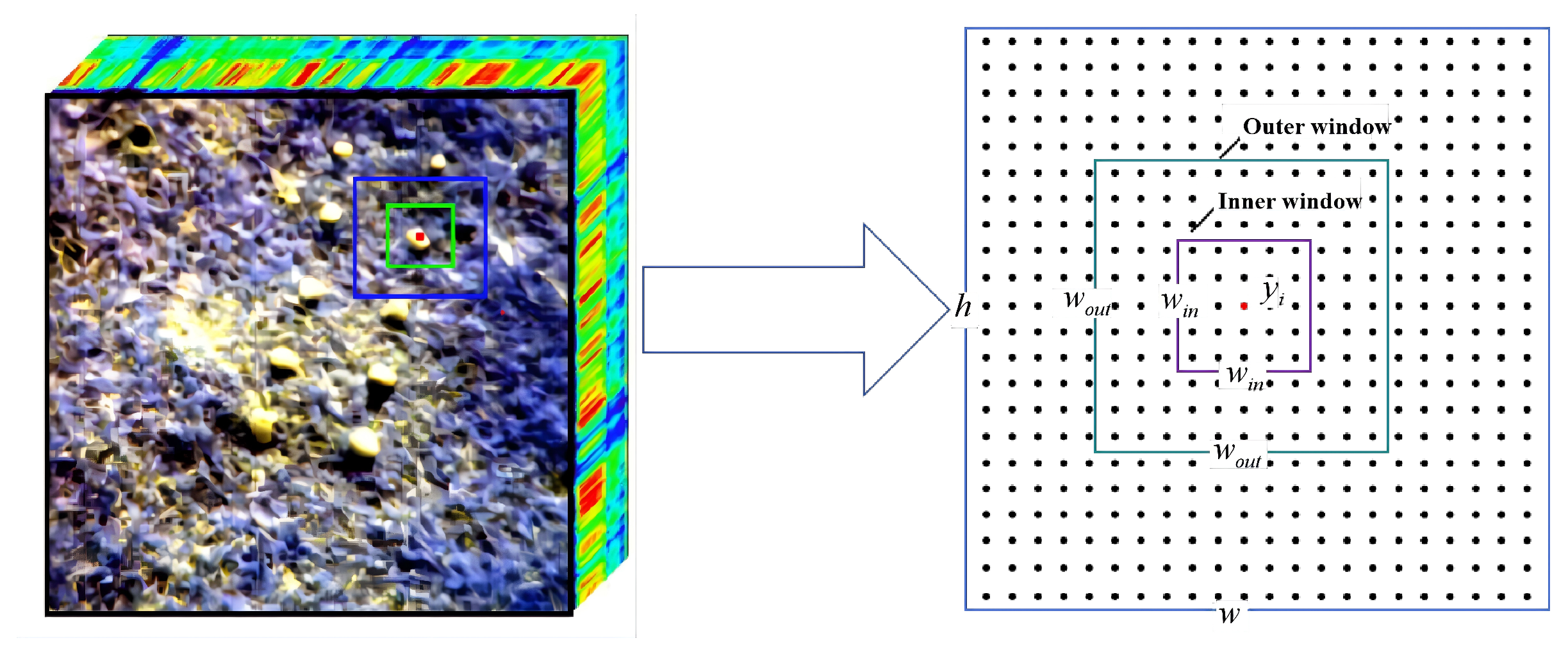
Figure 1. Schematic diagram of sliding dual-window model.
Remotesensing 17 03857 g001
Figure 2. Description of EMAPKCRD model.
Remotesensing 17 03857 g002
Figure 3. Window reconstruction model.
Remotesensing 17 03857 g003
Figure 4. Image scene descriptions. (a) False color image of the AVIRIS-I dataset. (b) False color image of the AVIRIS-II dataset. (c) False color image of the abu-urban-2 dataset. (d) False color image of the Cri dataset. (e) False color image of the Salinas-simulate dataset. (f) The ground truth map of the AVIRIS-I dataset. (g) The ground truth map of the AVIRIS-II dataset. (h) The ground truth map of the abu-urban-2 dataset. (i) The ground truth map of the Cri dataset. (j) The ground truth map of the Salinas-simulate dataset.
Remotesensing 17 03857 g004
Figure 5. Anomaly–background separation degree schematic.
Remotesensing 17 03857 g005
Figure 6. Impact of different k values on detection results.
Remotesensing 17 03857 g006
Figure 7. Color detection maps obtained by different algorithms for the AVIRIS-I dataset.
Remotesensing 17 03857 g007
Figure 8. Detection accuracy evaluation for the AVIRIS-I dataset. (a) ROC curves. (b) AUC values. (c) Anomaly–background separation degree schematic.
Remotesensing 17 03857 g008
Figure 9. Color detection maps obtained by different algorithms for the AVIRIS-II dataset.
Remotesensing 17 03857 g009
Figure 10. Detection accuracy evaluation for the AVIRIS-II dataset. (a) ROC curves. (b) AUC values. (c) Anomaly–background separation degree schematic.
Remotesensing 17 03857 g010
Figure 11. Color detection maps obtained by different algorithms for the abu-urban-2 dataset.
Remotesensing 17 03857 g011
Figure 12. Detection accuracy evaluation for the abu-urban-2 dataset. (a) ROC curves. (b) AUC values. (c) Anomaly–background separation degree schematic.
Remotesensing 17 03857 g012
Figure 13. Color detection maps obtained by different algorithms for the Cri dataset.
Remotesensing 17 03857 g013
Figure 14. Detection accuracy evaluation for the Cri dataset. (a) ROC curves. (b) AUC values. (c) Anomaly–background separation degree schematic.
Remotesensing 17 03857 g014
Figure 15. Color detection maps obtained by different algorithms for the Salinas simulation dataset.
Remotesensing 17 03857 g015
Figure 16. Detection accuracy evaluation for the Salinas simulation dataset. (a) ROC curves. (b) AUC values. (c) Anomaly–background separation degree schematic.
Remotesensing 17 03857 g016
Table 1. Running time (seconds).
DatasetCRDRCRDEMAPKCRD
AVIRIS-I8.65207.69740.6768
AVIRIS-II6.01945.25380.3962
Salinas-simulate11.589510.31513.0305
Cri80.083262.024922.7172
abu-urban-26.37665.81110.7924
Table 2. Auc Values.
DatasetCRDRCRDEMAPKCRD
AVIRIS-I0.98960.98750.9916
AVIRIS-II0.96310.97450.9813
Salinas-simulate0.93280.90560.9990
Cri0.91950.76720.9649
abu-urban-20.93520.84630.9989
Disclaimer/Publisher’s Note: The statements, opinions and data contained in all publications are solely those of the individual author(s) and contributor(s) and not of MDPI and/or the editor(s). MDPI and/or the editor(s) disclaim responsibility for any injury to people or property resulting from any ideas, methods, instructions or products referred to in the content.