Boosting SAR ATR Trustworthiness via ERFA: An Electromagnetic Reconstruction Feature Alignment Method

Highlights

What are the main findings?

• The integration of the frequency-domain electromagnetic reconstruction algorithm with image-domain cropping optimization achieves an effective balance between reconstruction accuracy and computational efficiency.
• The integration of electromagnetic reconstruction and feature alignment effectively enhances model robustness and suppresses background clutter in SAR ATR under varying operating conditions.

What are the implications of the main findings?

• Provides a trustworthy deep learning solution for SAR ATR by aligning electromagnetic reconstructions with image features, which helps mitigate overfitting to specific operating conditions.
• Provides evidence that utilizing target-related physical features significantly enhances the robustness, generalization and interpretability of deep learning-based SAR ATR.

Abstract

Deep learning-based synthetic aperture radar (SAR) automatic target recognition (ATR) methods exhibit a tendency to overfit specific operating conditions—such as radar parameters and background clutter—which frequently leads to high sensitivity against variations in these conditions. A novel electromagnetic reconstruction feature alignment (ERFA) method is proposed in this paper, which integrates electromagnetic reconstruction with feature alignment into a fully convolutional network, forming the ERFA-FVGGNet. The ERFA-FVGGNet comprises three modules: electromagnetic reconstruction using our proposed orthogonal matching pursuit with image-domain cropping-optimization (OMP-IC) algorithm for efficient, high-precision attributed scattering center (ASC) reconstruction and extraction; the designed FVGGNet combining transfer learning with a lightweight fully convolutional network to enhance feature extraction and generalization; and feature alignment employing a dual-loss to suppress background clutter while improving robustness and interpretability. Experimental results demonstrate that ERFA-FVGGNet boosts trustworthiness by enhancing robustness, generalization and interpretability.

1. Introduction

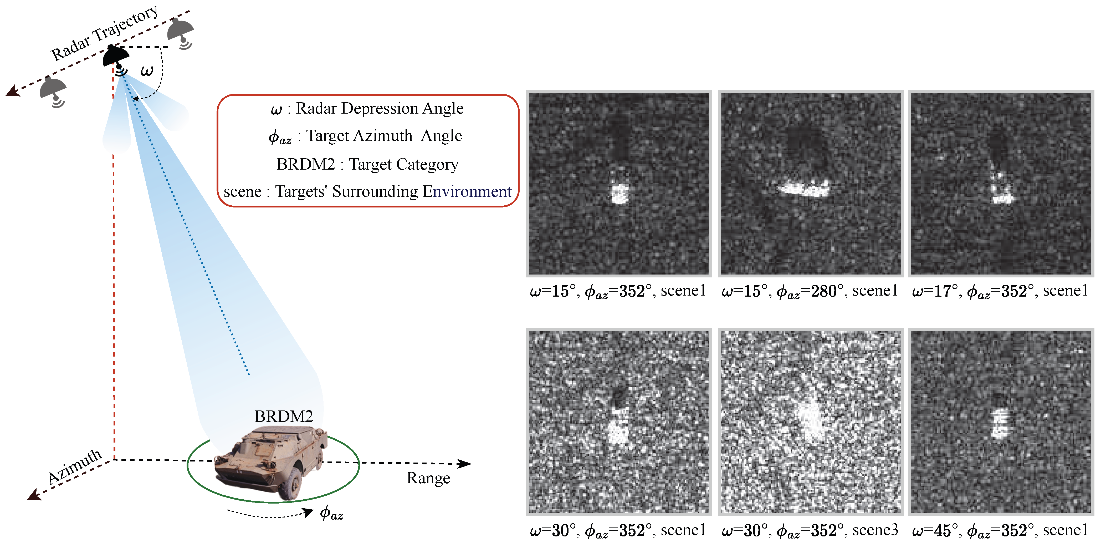
Synthetic aperture radar (SAR), with its all-weather and day-and-night operational advantages, has become a crucial means for remote sensing [1]. However, interpreting SAR images remains relatively challenging [2], because their characteristics are significantly shaped by operating conditions, including radar parameters, target signature and scene (e.g., background clutter). Moreover, the reflectivity of materials within commonly used radar frequency bands is not intuitive to human vision [3,4], as illustrated in Figure 1, which shows SAR images of a BRDM2 armored personnel carrier under different operating conditions.

In recent years, advances in deep learning have substantially propelled SAR target recognition, achieving accuracy rates exceeding 95% under standard operating conditions (SOCs)—where training and test sets exhibit homogeneous conditions. Numerous convolutional neural networks (CNNs), such as VGG [5] and ResNet [6], which originally designed for optical image recognition, have been successfully applied to SAR automatic target recognition (ATR). However, given the vast scale of optical image training samples and the substantial parameter sizes of these networks, directly applying them to SAR ATR with limited samples often induces overfitting. Chen et al. [7] proposed all convolutional networks (A-ConvNets), replacing fully connected layers with convolutional layers to reduce parameters, which demonstrates superior generalization in SAR ATR. The attention mechanism CNN (AM-CNN) [8] incorporates a lightweight convolutional block attention module (CBAM) after each convolutional layer in A-ConvNets for SAR ATR. Moreover, transfer learning has been leveraged to improve generalization under limited samples. Huang et al. [9,10] experimentally demonstrated that shallow features in transfer learning networks exhibit strong generality, whereas deep features are highly task-specific due to fundamental disparities in imaging mechanisms between optical and SAR modalities [11]. Building on ImageNet [12]-pretrained VGG16, Zhang et al. [13,14] redesigned deep classifiers while retaining shallow weights, proposing the reduced VGG network (RVGGNet) and the modified VGG network (MVGGNet), both achieving high recognition performance in SAR ATR. However, the operating condition space is vast, and when deep learning algorithms overfit specific operating conditions, models suffer from poor robustness and interpretability [15,16]. For instance, deep learning models may mainly depend on background clutter for classification [17,18]. Our previous experiments in [19] demonstrate that A-ConvNets, AM-CNN, and MVGGNet inevitably utilize background clutter as the primary decision-making basis, potentially compromising model robustness.

To enhance robustness, the speckle-noise-invariant network (SNINet) [20] employs $l_2$-regularized contrastive loss to align SAR images before and after despeckling, mitigating speckle noise effects. The contrastive feature alignment (CFA) method [21] employs a channel-weighted mean square error (CWMSE) loss to align deep features before and after background clutter perturbation, thereby reducing clutter dependency and enhancing robustness at the cost of compromised recognition performance. Although current deep learning SAR ATR methods demonstrate superior performance under SOC, their efficacy deteriorates under extended operating conditions (EOCs)—where substantial disparities exist between training and test sets. Researchers leverage the core characteristics of SAR imagery—complex-valued data encoding electromagnetic scattering mechanisms [22,23,24]—for high-performance target recognition. Multi-stream complex-valued networks (MS-CVNets) [25] decompose SAR complex images into real and imaginary components to fully exploit complex imaging features of SAR, constructing complex convolutional neural networks to extract richer information from SAR images and demonstrate superior performance under EOCs [25].

To further enhance robustness and interpretability, recent advancements incorporate electromagnetic features [22]—such as scattering centers [24] and attributed scattering centers (ASCs)—to enhance recognition performance across operating conditions. Zhang et al. [26] integrates the electromagnetic scattering feature with image features for SAR ATR. Liao et al. [27] design an end-to-end physics-informed interpretable network for scattering center feature extraction and target recognition under EOCs. Furthermore, Zhang et al. [13] enhances model recognition capability by concatenating deep features extracted by RVGGNet with independent ASC component patches. Huang et al. [28] integrate ASC components into a physics-inspired hybrid attention (PIHA) module within MS-CVNets, guiding the attention mechanism to focus on physics-aware semantic information in target regions and demonstrating superior recognition performance across diverse operating conditions. However, electromagnetic feature-based recognition methods are heavily reliant on reconstruction and extraction quality. Reconstruction and extraction algorithms are primarily divided into image-domain methods [29,30], which are computationally efficient but yield inaccurate results due to coarse segmentation, and frequency-domain approaches [31,32], which achieve higher precision but suffer from increased computational complexity that limits their practical application.

To address the issues mentioned above, we propose an electromagnetic reconstruction feature alignment (ERFA) method to boost model robustness, generalization and interpretability. ERFA leverages an orthogonal matching pursuit with image-domain cropping-optimization (OMP-IC) algorithm to reconstruct target ASC components, a fully convolutional VGG network (FVGGNet) for deep feature extraction, and a contrastive loss inspired by contrastive language-image pretraining (CLIP) [33,34] to align features between SAR images and reconstructed components. The main contributions of this paper are summarized as follows:

• A novel electromagnetic reconstruction and extraction algorithm named OMP-IC is proposed, which integrates image-domain priors into the frequency-domain OMP algorithm to optimally balance reconstruction accuracy and computational efficiency.
• A novel feature extraction network, termed FVGGNet, leverages the generic feature extraction capability of transfer learning with the inherent generalization of fully convolutional architectures, demonstrating enhanced discriminability and generalization.
• A dual-loss mechanism combining contrastive and classification losses is proposed that enables the ERFA module to suppress background clutter and enhance discriminative features, thus improving the robustness and interpretability of FVGGNet.

The rest of this article is organized as follows: Section 2 presents preliminaries on ASC reconstruction and extraction. The ERFA-FVGGNet architecture is presented in Section 3, followed by comprehensive experiments in Section 4 validating the method’s robustness, generalization and interpretability. Finally, Section 5 concludes this article.

2. Preliminaries

This section reviews the ASC model and the original frequency-domain OMP-based reconstruction and extraction algorithm that is foundational to our research.

2.1. Attributed Scattering Center Model

The ASC model proposed by Gerry et al. [29] employs a parameter set $\tilde{\mathsf{\Theta }}=\{A,\alpha ,x,y,L,\overline{\varphi },\gamma \}$, where A denotes complex intensity, $\alpha$ the frequency-dependent factor, $(x,y)$ range and azimuth coordinates, L the length, $\overline{\varphi }$ the inclination angle, and $\gamma$ the azimuth angle dependence factor. Constraints in modern radar systems, specifically a small signal-bandwidth-to-center-frequency ratio [35] and short azimuth observation time in SAR imaging [31,32], the modulation of scattering intensity by both the frequency-dependent factor $\alpha$ and the azimuth angle dependence factor $\gamma$ are minimal [31,32,35]. Meanwhile, the parameter set $\tilde{\mathsf{\Theta }}=\{A,x,y,L,\overline{\varphi }\}$ is more closely related to the physical structures of targets [36]. The SAR echoes $\tilde{s}\left(f,\varphi \right)$ are thus modeled as the coherent summation of multiple simplified ASCs

$$\begin{array}{cc}\hfill \tilde{s}\left(f,\varphi \right)& ={\displaystyle \sum _{i=1}^P}{z}_i·A_i·exp\left[{\displaystyle \frac{-j4\mathsf{\pi }f}{c}}\left(x_{i}cos\varphi +y_{i}sin\varphi \right)\right]\hfill \\ \hfill & ·sinc\left[{\displaystyle \frac{2\mathsf{\pi }f}{c}}{L}_{i}sin\left(\varphi -{\overline{\varphi }}_i\right)\right]+n(f,\varphi ),\hfill \end{array}$$

(1)

where f and $\varphi$ represent the radar frequency and azimuth angle, respectively; $f_c$ is the radar center frequency; $c=3\times {10}^8\mathrm{m}/\mathrm{s}$ denotes the speed of light; $z_i$ refers to the scattering coefficient; and $n(f,\varphi )$ corresponds to clutter and noise.

2.2. ASC Components Reconstruction and Extraction

The ASCs can be effectively reconstructed and extracted by solving

$$\hat{\mathbf{z}}=arg\underset{\mathbf{z}}{min}{\parallel \mathbf{z}\parallel }_0,\mathrm{s}.\mathrm{t}.{\parallel \tilde{\mathbf{s}}-\tilde{\mathbf{D}}\left(\tilde{\mathsf{\Theta }}\right)\mathbf{z}\parallel }_2\le \epsilon ,$$

(2)

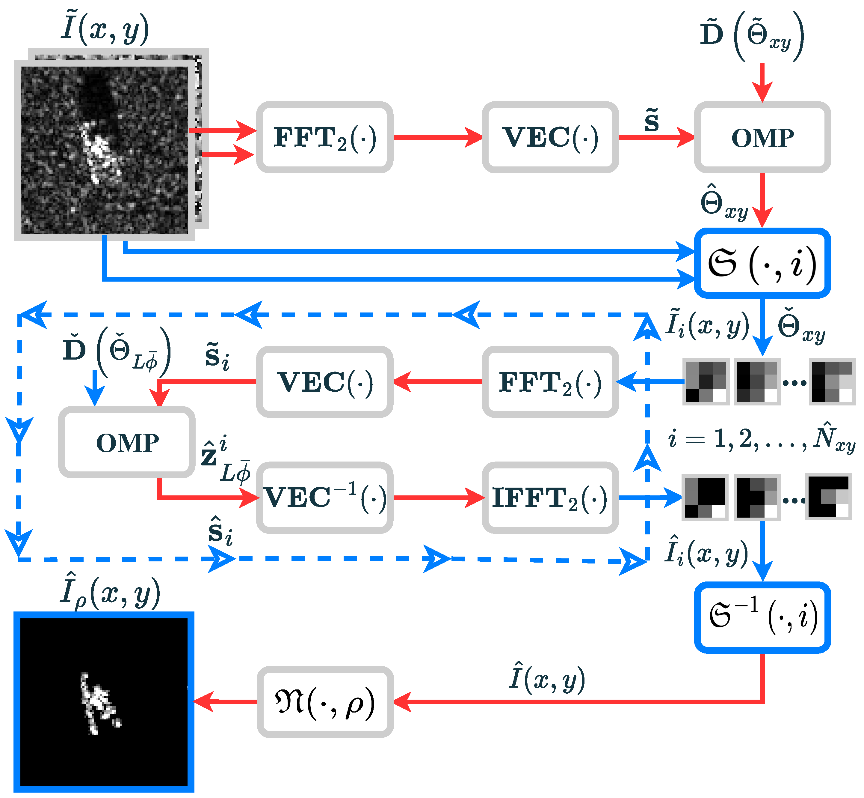
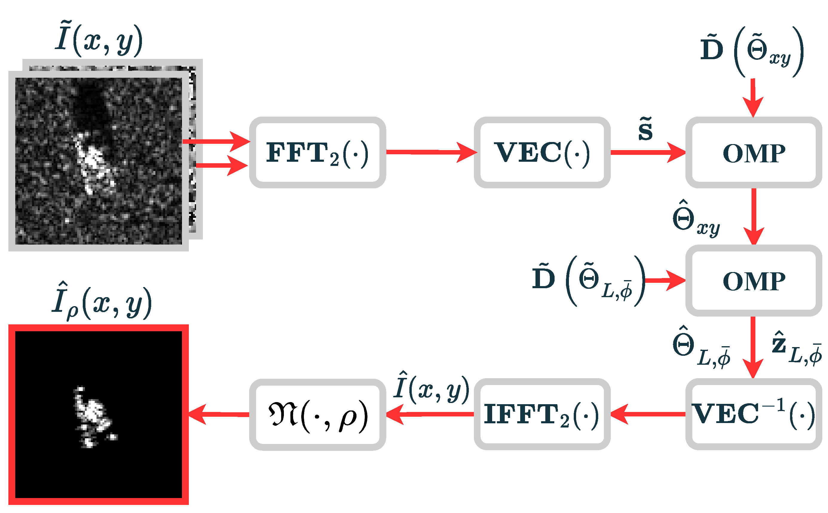
where ${\parallel ·\parallel }_0$ and ${\parallel ·\parallel }_2$ represent the $l_0$ norm and the $l_2$ norm, and $\epsilon$ is the estimated noise and clutter level. $\tilde{\mathbf{D}}\left(\tilde{\mathsf{\Theta }}\right)$ represents the dictionary matrix of the ASC parameter set $\tilde{\mathsf{\Theta }}$, $\mathbf{z}$ and $\tilde{\mathbf{s}}$ correspond to the vectorized forms of the scattering coefficients and SAR echoes. The approximate solutions of Equation (2) can be obtained through the OMP algorithm [31,32], as illustrated in Figure 2, which outlines the following 4 steps:

(1) Domain transformation: Converting the SAR image $\tilde{I}(x,y)$ from the image domain to the frequency-angle domain through 2D Fourier transform ${\mathrm{FFT}}_2(·)$ and in Figure 2 $\mathrm{VEC}(·)$ represents column-wise vectorization.

(2) $x,y$ estimation: Constructing the position parameter dictionary $\tilde{\mathbf{D}}\left({\tilde{\mathsf{\Theta }}}_{xy}\right)$ and solving the sparse optimization problem as Equation (2) using the OMP algorithm [31], the scattering coefficients ${\hat{\mathbf{z}}}_{xy}$ and the parameter set ${\hat{\mathsf{\Theta }}}_{xy}$ can be obtained.

(3) $L,\overline{\varphi }$ estimation: Based on the estimated position parameter set ${\hat{\mathsf{\Theta }}}_{xy}$, construct the $L,\overline{\varphi }$ dictionary $\tilde{\mathbf{D}}\left({\tilde{\mathsf{\Theta }}}_{L\overline{\varphi }}\right)$; the scattering coefficients ${\hat{\mathbf{z}}}_{L\overline{\varphi }}$ and the parameter set ${\hat{\mathsf{\Theta }}}_{L\overline{\varphi }}$ can then be derived accordingly.

(4) SAR target components reconstruction: The iteration stopping criteria for the OMP algorithm [31] are

$${\epsilon }_R={∥{\displaystyle \frac{{\hat{\mathbf{s}}}_k^H·{\hat{\mathbf{s}}}_k-{\hat{\mathbf{s}}}_{k-1}^H·{\hat{\mathbf{s}}}_{k-1}}{{\tilde{\mathbf{s}}}^H·\tilde{\mathbf{s}}}}∥}_2,$$

(3)

where ${\hat{\mathbf{s}}}_k=\hat{\mathbf{D}}\left({\hat{\mathsf{\Theta }}}^k\right)·{\hat{\mathbf{z}}}^k$ represents the reconstructed SAR echoes of the k-th iteration and H denotes the Hermitian operator. As shown in Figure 2, the reconstructed echoes are reshaped into their original matrix form by the inverse vectorization operation ${\mathrm{VEC}}^{-1}(·)$, then transformed to the image domain $\hat{I}(x,y)$ via 2D inverse Fourier transform ${\mathrm{IFFT}}_2(·)$. To suppress background clutter and enhance target feature representation, an activation function $\mathfrak{N}(·,\rho )$ with threshold $\rho$ is applied to focus on target regions [28].

$$\begin{array}{cc}\hfill {\hat{I}}_{\rho }(x,y)& =\mathfrak{N}(\hat{I}(x,y),\rho )=\left\{\begin{array}{cc}|\hat{I}(x,y)|,\hfill & |\hat{I}(x,y)|\ge \rho \hfill \\ 0,\hfill & |\hat{I}(x,y)|<\rho \hfill \end{array}\right..\hfill \end{array}$$

(4)

The selection of $\rho$ and ${\epsilon }_R$ critically governs reconstruction fidelity, with detailed parameter analyses in Section 4.3. By incorporating radar parameters, the ASC model enables radar data measurement analysis and provides physical measurement for target recognition, data compression/reconstruction, and scattering property analysis.

3. Proposed Methods

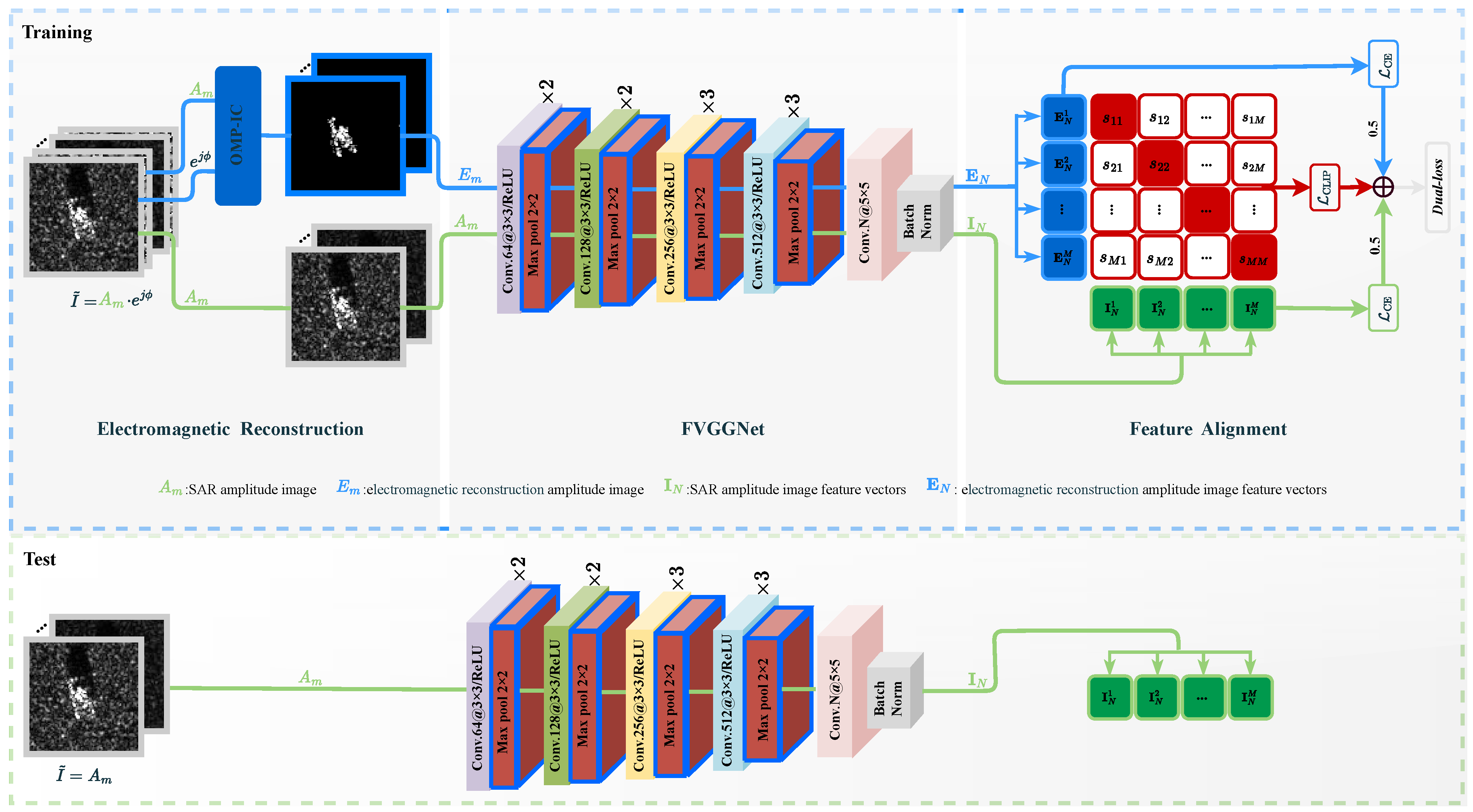
This section introduces the proposed ERFA-FVGGNet as shown in Figure 3 for trustworthy SAR target recognition. $\tilde{I}$ denotes the SAR complex image, with $A_m$ and $e^{j\varphi }$ representing its amplitude and phase, respectively. The electromagnetic reconstruction module based on OMP-IC is described in Section 3.1, which generates source domain data for feature alignment. The FVGGNet is presented in Section 3.2.1, extracting deep features from both SAR images and electromagnetic reconstructions. Finally, applying the clip contrastive loss to align deep SAR image features with deep electromagnetic reconstruction features while suppressing background clutter is detailed in Section 3.2.2.

3.1. Electromagnetic Reconstruction

The original OMP reconstruction algorithm introduced in Section 2.2 suffers from substantial computational load and memory consumption, resulting in low computational efficiency. Specifically, for ($L,\overline{\varphi }$) estimation, assuming the SAR image is $\tilde{I}(x,y)\in {\mathbb{C}}^{M^2}$, with the estimated ($x,y$) parameter set size ${\hat{N}}_{xy}=\mathrm{card}\left({\hat{\mathsf{\Theta }}}_{xy}\right)$ and the ($L,\overline{\varphi }$) parameter set size ${\tilde{N}}_{L\overline{\varphi }}=\mathrm{card}\left({\tilde{\mathsf{\Theta }}}_{L\overline{\varphi }}\right)$, the computational speed of the OMP algorithm is primarily determined by atom selection and matrix inversion. The dictionary for solving ($L,\overline{\varphi }$) contains ${\hat{N}}_{xy}\times {\tilde{N}}_{L\overline{\varphi }}$ atoms, and each iteration of the OMP involves computational complexity of $O\left(M^2\times {\hat{N}}_{xy}\times {\tilde{N}}_{L\overline{\varphi }}\right)$ for atom selection and pseudo-inverse computation of $M^2$-sized matrices, making each iteration computationally intensive.

To reduce computation, block compressed sensing [37] divides the entire image into multiple independent uniform blocks and reconstructs all blocks using the same dictionary, effectively reducing storage pressure and computational complexity. However, this disjoint blocking severs inter-block correlations, causing blocking artifacts that degrade reconstruction quality. To simultaneously reduce computation and suppress blocking artifacts [38], we propose the OMP-IC algorithm to preserve overlapping regions between adjacent blocks to enhance inter-block correlations.

Specifically, the OMP-IC, as illustrated in Figure 4, shares the step (1) and (2) with the original OMP-based reconstruction and extraction method in Section 2.2. Prior to estimating ($L,\overline{\varphi }$), the original SAR image is cropped into overlapping blocks in the image domain, centered on the estimated ($x,y$) coordinates, preserving inter-block correlations to suppress artifacts. This arises from the translational property of ASCs in the image domain [39], where two ASCs with identical parameters except $x,y$ positions exhibit identical waveforms

$$\tilde{I}(x-\Delta x,y-\Delta y)=\tilde{I}(x,y).$$

(5)

Meanwhile, ASCs exhibit an additive property in the image domain [39], meaning that a scattering center of length L can be represented by the linear superposition of multiple ASCs

$$\tilde{I}\left(x,y;{\tilde{\mathsf{\Theta }}}_L\right)={\displaystyle \sum _{i=1}^P}{\displaystyle \frac{L_i}{L}}\tilde{I}\left(x,y;{\tilde{\mathsf{\Theta }}}_{L_i}\right),$$

(6)

where

$$L=L_1+L_2+\cdots +L_P.$$

(7)

The translational property of ASCs in the image domain allows all cropped image blocks to retain identical position parameters, enabling dictionary reuse and reducing memory requirements for dictionary storage. Simultaneously, the additive property ensures that a complete ASC can be represented through the linear superposition of multiple cropped ASCs, thereby validating the feasibility of image-domain cropping.

The proposed OMP-IC specifically modifies step (3) in Section 2.2: using ($x,y$) position parameters estimated in (2), crop the full SAR image $\tilde{I}(x,y)\in {\mathbb{C}}^{M^2}$ into ${\hat{N}}_{xy}$ image blocks of size $N^2$, centered at each ASC location, with overlapping cropping between adjacent blocks. The overlapping regions maintain structural continuity through additive property, enabling seamless block fusion during the next step,

$${\tilde{I}}_i(x,y)=\mathfrak{S}\left(\tilde{I}(x,y),i\right),(i=1,2,\cdots ,{\hat{N}}_{xy}),$$

(8)

where ${\tilde{I}}_i(x,y)\in {\mathbb{C}}^{N^2}$, and $\mathfrak{S}(·,i)$ denotes the image cropping operation centered at the locations of the i-th ASC. Subsequently, echoes ${\tilde{\mathbf{s}}}_i$ ($i=1,2,\cdots ,{\hat{N}}_{xy}$) are generated for each image block as shown in Figure 4, where each block contains at least one ASC. Leveraging the translational property, all ASC positions within a block are represented by a common overcomplete position parameter set ${\check{\mathsf{\Theta }}}_{xy}$, with cardinality $N^2=\mathrm{card}\left({\check{\mathsf{\Theta }}}_{xy}\right)$. Thus, the dictionary $\check{\mathbf{D}}\left({\check{\mathsf{\Theta }}}_{L\overline{\varphi }}\right)$ is then repeatedly used for the OMP algorithm to estimate the scattering coefficients ${\hat{\mathbf{z}}}_{L\overline{\varphi }}^i(i=1,2,\cdots ,{\hat{N}}_{xy})$.

The OMP-IC specifically modifies step (4) in Section 2.2 as follows: sequentially reconstructing the echoes ${\hat{\mathbf{s}}}_i,(i=1,2,\cdots ,{\hat{N}}_{xy})$, transforming them to the image-domain via ${\mathrm{VEC}}^{-1}(·)$ and ${\mathrm{IFFT}}_2(·)$ to obtain ${\hat{I}}_i(x,y),(i=1,2,\cdots ,{\hat{N}}_{xy})$, and repositioning all reconstructed blocks into their original locations within a blank image matching the dimensions of the original SAR image

$$\hat{I}(x,y)={\mathfrak{S}}^{-1}\left({\hat{I}}_i(x,y),i\right),(i=1,2,\cdots ,{\hat{N}}_{xy}),$$

(9)

where ${\mathfrak{S}}^{-1}(·,i)$ denotes the image block restoration operation. Finally, passing $\hat{I}(x,y)$ through the activation function shown in Equation (4) to obtain the reconstructed ${\hat{I}}_{\rho }(x,y)$.

By incorporating image-domain cropping, the number of dictionary atoms required for estimating ($L,\overline{\varphi }$) reduces to $N^2\times {\tilde{N}}_{L\overline{\varphi }}$, where $N^2\ll {\hat{N}}_{xy}\ll M^2$. The computational complexity for atom selection per OMP iteration becomes $O\left(N^2\times N^2\times {\tilde{N}}_{L\overline{\varphi }}\right)$, with only the pseudo-inverse calculation of an $N^2$-sized matrix required each iteration. As a result, the OMP-IC enables efficient SAR target component reconstruction.

3.2. Feature Extraction and Alignment

To enhance feature discriminability and suppress background clutter via electromagnetic reconstruction results from OMP-IC, a feature alignment framework integrating pretrained FVGGNet with CLIP contrastive loss is proposed.

3.2.1. FVGGNet

As mentioned in Section 1, shallow structures of pretrained models can extract general information from images, with their generalization stemming from pervasive similarities across images. In contrast, deep layers exhibit strong dependence on domain-specific characteristics, resulting in redundant parameters. Simultaneously, SAR ATR often suffers from limited training samples, causing models to easily overfit and impair generalization. A-ConvNets [7] mitigates this by removing the parameter-heavy fully connected layers, thereby reducing model complexity and enhancing generalization [40]. Furthermore, small convolutional kernels (e.g., $3\times 3$ or $5\times 5$) typically exhibit superior feature extraction capabilities [41].

Therefore, we propose a fully convolutional VGG network (FVGGNet), which leverages the feature extraction advantages of pretrained shallow networks to improve model generalization under limited samples by replacing fully connected layers with small convolutional kernel layers, as illustrated in Figure 3 and

Table 1. The structure of FVGGNet.

Layers	Type	Kernel Size	Stride	Output Size
0	Input	-	-	$88\times 88$
1	Conv	$3\times 3\times 64$	1	$88\times 88$
2	Conv	$3\times 3\times 64$	1	$88\times 88$
3	Maxpool	$2\times 2$	2	$44\times 44$
4	Conv	$3\times 3\times 128$	1	$44\times 44$
5	Conv	$3\times 3\times 128$	1	$44\times 44$
6	Maxpool	$2\times 2$	2	$22\times 22$
7	Conv	$3\times 3\times 256$	1	$22\times 22$
8	Conv	$3\times 3\times 256$	1	$22\times 22$
9	Conv	$3\times 3\times 256$	1	$22\times 22$
10	Maxpool	$2\times 2$	2	$11\times 11$
11	Conv	$3\times 3\times 512$	1	$11\times 11$
12	Conv	$3\times 3\times 512$	1	$11\times 11$
13	Conv	$3\times 3\times 512$	1	$11\times 11$
14	Maxpool	$2\times 2$	2	$5\times 5$
15	Conv	$5\times 5\times N$	1	$1\times 1\times N$
16	BatchNorm	-	-	$1\times 1\times N$

, “Conv”, “MaxPool”, and “BatchNorm” denote the convolutional layers, max-pooling layers, and batch normalization layers, respectively. This network selects the first 14 layers of the VGG16 network pre-trained on the ImageNet dataset [12], utilizing the shallow structure of the pre-trained network to extract features from SAR images. Subsequently, a $5\times 5$ convolutional kernel with a stride of 1 followed by batch normalization serves as the classifier, where N represents the number of target categories, enabling target classification.

3.2.2. Feature Alignment

As shown in Figure 3, a batch of SAR amplitude images and electromagnetic reconstruction amplitude images are input into the FVGGNet to extract their image features ${\mathbf{I}}_N=\{{\mathbf{I}}_N^1,{\mathbf{I}}_N^2,\cdots ,{\mathbf{I}}_N^M\}$ and electromagnetic reconstruction features ${\mathbf{E}}_N=\{{\mathbf{E}}_N^1,{\mathbf{E}}_N^2,\cdots ,{\mathbf{E}}_N^M\}$. Here, N denotes the number of target categories (i.e., the length of each feature vector), and M denotes the batch size. To suppress interference from background clutter and ensure recognition performance, the contrastive loss [33] is introduced. The contrastive loss first computes the normalized cosine similarity between the image features and electromagnetic reconstruction features across the batch

$$s_{i,j}={\displaystyle \frac{{\mathbf{I}}_N^i·{\mathbf{E}}_N^j}{{\parallel {\mathbf{I}}_N^i\parallel }_2{\parallel {\mathbf{E}}_N^j\parallel }_2}},(i,j=1,2,\cdots ,M).$$

(10)

The bidirectional contrastive loss is then applied, where the image feature ${\mathbf{I}}_N^i$ only matches the electromagnetic reconstruction feature ${\mathbf{E}}_N^i$ among all electromagnetic reconstruction features

$${\mathcal{L}}_{{\mathbf{I}}_N\to {\mathbf{E}}_N}=-{\displaystyle \frac{1}{M}}{\displaystyle \sum _{i=1}^M}log{\displaystyle \frac{exp\left(s_{i,i}/\tau \right)}{{\sum }_{j=1}^{N}exp\left(s_{i,j}/\tau \right)}};$$

(11)

Similarly, the electromagnetic reconstruction feature ${\mathbf{E}}_N^j$ only matches the image feature ${\mathbf{I}}_N^j$ among all image features

$${\mathcal{L}}_{{\mathbf{E}}_N\to {\mathbf{I}}_N}=-{\displaystyle \frac{1}{M}}{\displaystyle \sum _{j=1}^M}log{\displaystyle \frac{exp\left(s_{j,j}/\tau \right)}{{\sum }_{i=1}^{N}exp\left(s_{i,j}/\tau \right)}};$$

(12)

Here, $\tau \in [0.01,100]$ is a learnable temperature coefficient used to adjust the alignment strength between features. When $\tau$ is smaller, tighter alignment occurs between image features and electromagnetic features. This may lead to over-penalization, which increases the distance between different samples of the same target in the feature space, potentially causing model overfitting. Conversely, when $\tau$ is larger, feature alignment becomes more relaxed. While this avoids excessive penalization, samples from different targets may lack sufficient discrimination in the feature space, compromising model recognition performance [42]. Ultimately, the contrastive loss is

$${\mathcal{L}}_{CLIP}={\displaystyle \frac{1}{2}}\times ({\mathcal{L}}_{{\mathbf{I}}_N\to {\mathbf{E}}_N}+{\mathcal{L}}_{{\mathbf{E}}_N\to {\mathbf{I}}_N});$$

(13)

Here, we employ the learnable temperature coefficient $\tau$ to adaptively regulate feature alignment strength and control recognition efficiency. Hence, the dual loss is defined as

$$\mathcal{L}={\displaystyle \frac{1}{2}}\times ({\mathcal{L}}_{CE}({\mathbf{E}}_N,{\mathbf{Y}}_N)+{\mathcal{L}}_{CE}({\mathbf{I}}_N,{\mathbf{Y}}_N))+{\mathcal{L}}_{CLIP},$$

(14)

where ${\mathcal{L}}_{CE}$ denotes the cross-entropy loss function for target classification, ${\mathbf{Y}}_N=\{{\mathbf{Y}}_N^1,{\mathbf{Y}}_N^2,\cdots ,{\mathbf{Y}}_N^M\}$ are the ground-truth labels

$${\mathcal{L}}_{CE}({\mathbf{E}}_N,{\mathbf{Y}}_N)=-{\displaystyle \frac{1}{M}}\sum _{i=1}^M{\mathbf{Y}}_N^{i}log\left({\mathbf{E}}_N^i\right),$$

(15)

Similarly, ${\mathcal{L}}_{CE}({\mathbf{I}}_N,{\mathbf{Y}}_N)$ can be obtained. The proposed dual-loss $\mathcal{L}$ is designed to adaptively adjust the alignment between electromagnetic reconstruction features and image features, suppress model overfitting to background clutter, and preserve recognition accuracy.

4. Experimental Results and Discussion

In this section, the specific dataset and experimental settings are first outlined in Section 4.1. The evaluation metrics are briefly introduced in Section 4.2. The parameter analysis of the proposed OMP-IC algorithm is compared with the original OMP method in Section 4.3. Robustness, generalization, and interpretability are assessed in comparison with various methods in Section 4.4. Finally, ablation experiments are subsequently conducted in Section 4.5 to validate the effectiveness of each module in ERFA-FVGGNet.

4.1. Dataset and Experimental Settings

4.1.1. Dataset Overview

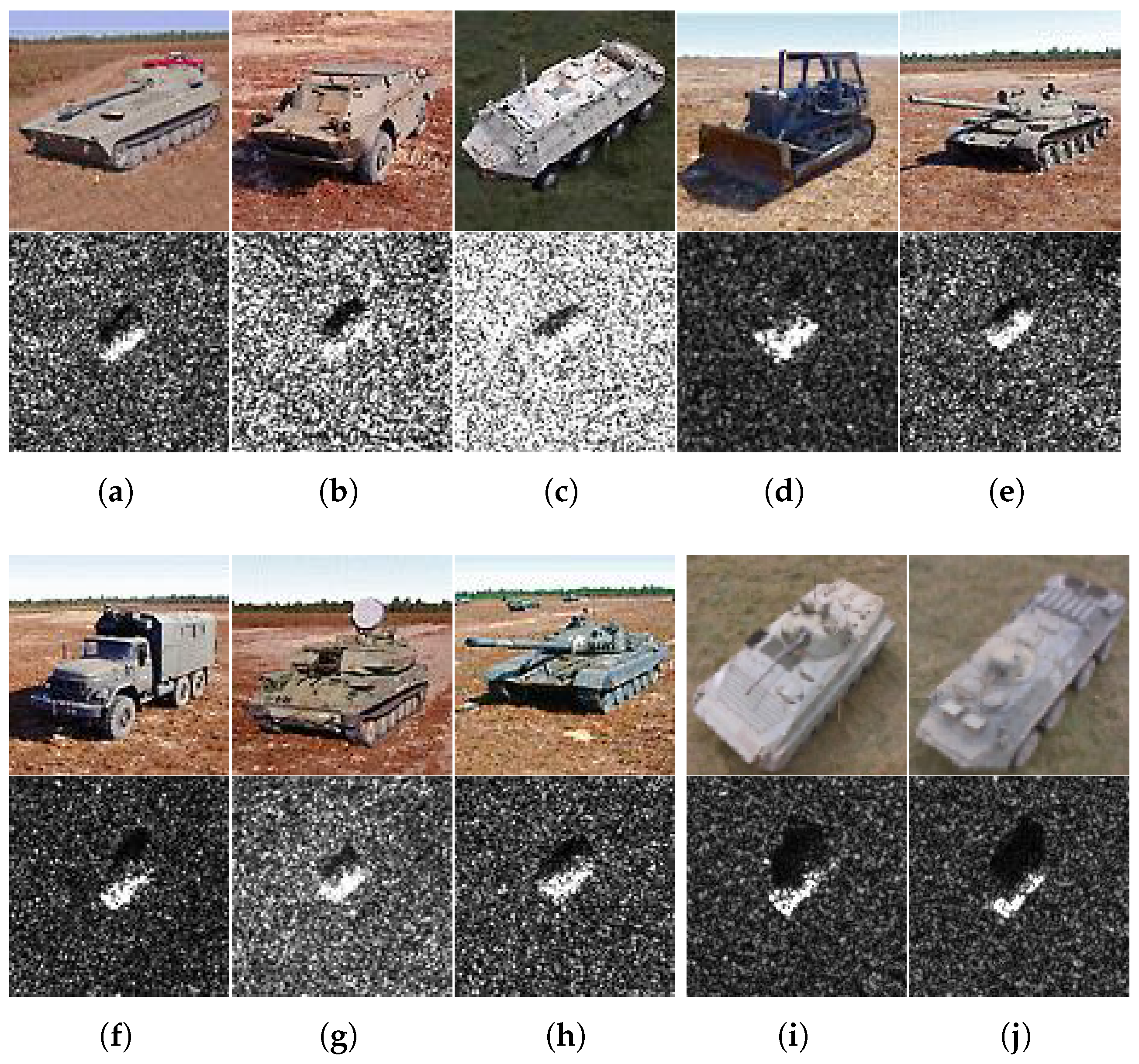
The moving and stationary target acquisition and recognition (MSTAR) dataset originates from the MSTAR program [43] conducted by the Defense Advanced Research Projects Agency (DARPA) and the Air Force Research Laboratory (AFRL) between 1995 and 1996. The SAR system used for data acquisition was specifically for the MSTAR project by Sandia National Laboratory (SNL). The imaging parameters are detailed in

Table 2. SAR imaging parameters.

Parameters	MSTAR	OpenSARShip
Imaging mode	Spotlight	Interferometric wide
Polarization	HH	VV
Platform	Airborne	Spaceborne
Center frequency ($\mathrm{GHz}$)	9.6	5.4
Bandwidth ($\mathrm{GHz}$)	0.591	0.065
Range resolution ($\mathrm{m}$)	0.3047	2.3
Azimuth resolution ($\mathrm{m}$)	0.3047	14.1
Depression angle (∘)	15, 17, 30, 45	32.9, 38.3, 43.1
Azimuth angle (∘)	0∼360	0∼360

. The targets include ten Soviet military vehicles: the 2S1 howitzer, BMP2 infantry fighting vehicle, BRDM2 armored personnel carrier, BTR60 armored personnel carrier, BTR70 armored personnel carrier, D7 bulldozer, T62 tank, T72 tank, ZIL131 truck, and ZSU234 gun. Figure 5 displays the optical and the corresponding SAR images of these targets. The MSTAR dataset encompasses two distinct operating conditions: the SOC, characterized by similar imaging parameters, target classes, and scenes across training and test sets; and the EOCs, which exhibit significant variations in these aspects. Our experiments systematically evaluate depression angle discrepancies, target configuration and version variations, and scene transitions.

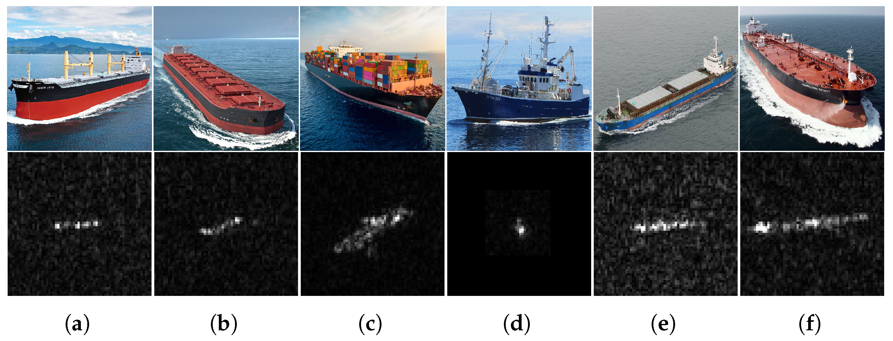
The OpenSARShip dataset (including OpenSARShip1.0 [44], OpenSARShip2.0 [45]) is a public benchmark curated by Shanghai Jiao Tong University and comprises SAR ship images from Sentinel-1 satellites. For our study, we utilized 35 single look complex (SLC) products in VV polarization, covering six ship categories: bulk carriers, cargo, container ships, fishing, general cargo, and tankers. Owing to its complex maritime scenes, the OpenSARShip dataset offers high representativeness of real-world operating conditions. The imaging parameters are detailed in Table 2 and Figure 6 displays optical images alongside their corresponding SAR representations for these targets.

4.1.2. Hyperparameter Settings

The ImageNet-pretrained weights are used as initialization for FVGGNet. The network is trained with the Nadam [46] optimizer, initial learning rate $5\times {10}^{-4}$, exponential decay factor 0.99 (learning rate decays to 99% of previous value per iteration), CLIP contrastive loss with initial temperature coefficient 10, batch size 32 and 100 training epochs. All experiments were conducted on an Intel i9-10920X CPU with an NVIDIA RTX 2080 Ti GPU.

4.1.3. MSTAR SOC

Under SOC, both the training and test sets comprise ten classes of targets with consistent configurations, versions, and scenes, while maintaining similar depression angles between sets as

Table 3. MSTAR SOC training and test set samples.

Class	Serial	Scene	Training		Test
			Dep.	No.	Dep.	No.
2S1	B01	1	17°	299	15°	274
BMP2	9563			233		195
BRDM2	E71			298		274
BTR60	7532			256		195
BTR70	c71			233		196
D7	13015			299		274
T62	A51			299		273
T72	132			232		196
ZIL131	E12			299		274
ZSU234	d08			299		274
Total				2747		2425

.

4.1.4. MSTAR EOC-Depression

The depression angle significantly impacts the scattering properties of both targets and background clutter. 2S1, BRDM2, T72 and ZSU234 are selected to train at ${17}^{\circ }$ and test at ${30}^{\circ }$ to evaluate robustness across depression angles. As shown in

Table 4. MSTAR EOC-Depression training and test set samples.

Class	Serial	Scene	Training		Test
			Dep.	No.	Dep.	No.
2S1	B01	1	${17}^{\circ }$	299	${30}^{\circ }$	288
BRDM2	E71			298		288
T72	A64			299		288
ZSU234	d08			299		287
total				1195		1151

, the EOC-Depression test set only modifies the depression angle, with all other settings consistent with the training set.

4.1.5. MSTAR EOC-Version

The MSTAR dataset contains multiple version variants of BMP2 and T72 samples. For cross-version generalization assessment, the EOC-Version alters the target version while maintaining other settings specified in

Table 5. MSTAR EOC-Version training and test set samples.

Class	Serial	Scene	Training		Test
			Dep.	No.	Dep.	No.
BMP2	9563	1	${17}^{\circ }$	233	${15}^{\circ },{17}^{\circ }$	-
	9566			-		428
	C21			-		429
BRDM2	E71			298		-
BTR70	C71			233		-
T72	132			232		-
	812			-		426
	A04			-		573
	A05			-		573
	A07			-		573
	A10			-		567
Total				996		2710

.

4.1.6. MSTAR EOC-Configuration

The MSTAR dataset provides various T72 configurations through distinct combinations of side skirts, fuel tanks, and reactive armor. To validate generalization under configuration variations, the EOC-Configuration maintains identical settings between training and test sets except for target configurations as in

Table 6. MSTAR EOC-Configuration training and test set samples.

Class	Serial	Scene	Training		Test
			Dep.	No.	Dep.	No.
BMP2	9563	1	${17}^{\circ }$	233	${15}^{\circ },{17}^{\circ }$	-
BRDM2	E71			298		-
BTR70	C71			233		-
T72	132			232		-
	S7			-		419
	A32			-		572
	A62			-		573
	A63			-		573
	A64			-		573
Total				996		3569

.

4.1.7. MSTAR EOC-Scene

The MSTAR dataset was collected across three distinct sites: New Mexico, northern Florida, and northern Alabama. Although all sites are characterized by grassland terrain, variations in grass height, density, and vegetation/surface moisture alter the electromagnetic scattering characteristics and the distribution of background clutter. For the EOC-Scene, the training and test sets share identical settings—except for the scenes. Here, labels 1, 2, and 3 denote three distinct grassland conditions (Grass 1, Grass 2, and Grass 3), with specifications detailed in

Table 7. MSTAR EOC-Scene training and test set samples.

Class	Serial	Dep.	Training		Test
			Scene	No.	Scene	No.
BRDM2	E71	${30}^{\circ }$, ${45}^{\circ }$	1	591	3	253
T72	A64			590		253
ZSU234	d08			591	2	237
Total				1772		743

.

4.1.8. MSTAR OFA

To further evaluate the cross-operating robustness and generalization of deep learning models, an once-for-all (OFA) evaluation protocol was proposed in [28] using the MSTAR dataset, introducing a more challenging task. OFA refers to a process where a model trained on a single training set can be directly evaluated on multiple test sets with different data distributions, distinguishing it from SOC/EOC evaluations that require separate training sets for each test set; this design enables more effective assessment. The OFA contains three test conditions: OFA-1, where the test set shares identical settings with the training set, including the same classes, serial numbers, scenes, and similar depression angles; OFA-2, where the test set extends OFA-1 by adding 4 variants of BMP2 and T72 to evaluate model generalization against configurations and versions variants; and OFA-3, the test set comprises a mixture of 2S1, BRDM2, and ZSU234, each exhibiting depression angles of ${15}^{\circ }$, ${30}^{\circ }$ and ${45}^{\circ }$, with the BRDM2 and ZSU234 additionally exhibiting variations in scene conditions, creating significant distribution shifts to the training set to test cross-conditions robustness and generalization. As shown in

Table 8. MSTAR OFA training and test set samples.

Class	Serial	Training			OFA-1			OFA-2			OFA-3
		Scene	Dep.	No.	Scene	Dep.	No.	Scene	Dep.	No.	Scene	Dep.	No.
2S1	B01	1	${17}^{\circ }$	299	1	${15}^{\circ }$	274	1	${15}^{\circ }$	274	1/1/1	${15}^{\circ }$$/{30}^{\circ }$$/{45}^{\circ }$	274/288/303
BMP2	9563			233			195			195			-
	9566			-			-			196			-
	C21			-			-			196			-
BRDM2	E71			298			274			274	1/1,3/1,3		274/420/423
BTR70	C71			233			196			196			-
BTR60	7532			256			195			195			-
D7	13015			299			274			274			-
T62	A51			299			273			273			-
T72	132			232			196			196			-
	812			-			-			195			-
	S7			-			-			191			-
ZIL131	E12			299			274			274			-
ZSU234	d08			299			274			274	1/1,2/1,2		274/406/422
Total				2747			2425			3203			3084

, ${17}^{\circ }$ depression angle samples serve as training data for OFA-1, OFA-2, and OFA-3.

4.1.9. OpenSARShip Dataset

The OpenSARShip dataset used in this paper consists of 3525 image slices, divided into training and test sets at a ratio of 70% to 30%. Following the data partitioning scheme described in [34], both three-class and six-class classification configurations are provided, as shown in

Table 9. OpenSARShip for three-class and six-class training and test set samples.

Class	Three-Class		Six-Class
	Training	Test	Training	Test
Bulk carrier	410	177	410	177
Cargo	-	-	893	384
Container ship	536	231	536	231
Fishing	-	-	164	71
General cargo	-	-	191	89
Tanker	265	114	265	114
Total	1211	522	2459	1066

. Since target areas typically occupy only a small portion of the original SAR image, all samples are center-cropped to $64\times 64$ pixels [34] and then padded to $88\times 88$ pixels. The image slices were acquired from significant ports with high traffic density, including Shanghai Port, Singapore Port, Thames Port, and Yokohama Port. The complex background clutter, diverse scene conditions, and considerable intra-class shape variability collectively create a challenging and diverse set of operating conditions, making the dataset well-suited for evaluating model robustness and generalization.

4.2. Evaluation Metrics

4.2.1. Overall Accuracy

To evaluate the recognition performance of the proposed method, the overall accuracy (OA) [28,47] is employed

$$\mathrm{OA}={\displaystyle \frac{\mathrm{TP}+\mathrm{TN}}{\mathrm{TP}+\mathrm{TN}+\mathrm{FP}+\mathrm{FN}}},$$

(16)

where TP is true positives, TN is true negatives, FP is false positives, and FN is false negatives.

4.2.2. Weighted Composition Ratio Statistic

Our previous work [19] proposed the weighted composition ratio statistic (WCRS) for quantitatively evaluating model overinterpretation. We employ distinct segmentation strategies for the two datasets: the MSTAR images are partitioned into three regions (target, shadow, and background) using the SARBake dataset [48], while the OpenSARShip images are segmented into target and background regions using the OTSU method [49]. We identify key regions for model classification in each sample through various feature attribution methods [16] and the OTSU segmentation methods. Based on the proposed necessity–sufficiency index (NSI), we then locate the model’s decision-making basis from these key regions and calculate the proportion of target, shadow, and background regions in the decision-making basis by treating NSI as a weighted average weight. The Background WCRS is

$${\mathrm{WCRS}}_{\mathrm{bg}}={\displaystyle \frac{{\sum }_{k=1}^K{\mathrm{NSI}}_k\times P_{\mathrm{bg}}^k}{{\sum }_{k=1}^K{\mathrm{NSI}}_k}};$$

(17)

Here, K is the number of samples in the dataset, and $P_{\mathrm{bg}}$ is the composition ratio of the background within the decision-making basis. Similarly, $WCR{S}_{\mathrm{tg}}$ for the target and $WCR{S}_{\mathrm{sd}}$ for the shadow can be calculated. By computing the WCRS of the identification model for all samples in the dataset, the model’s overinterpretation can be quantitatively evaluated.

4.3. Analysis of OMP-IC

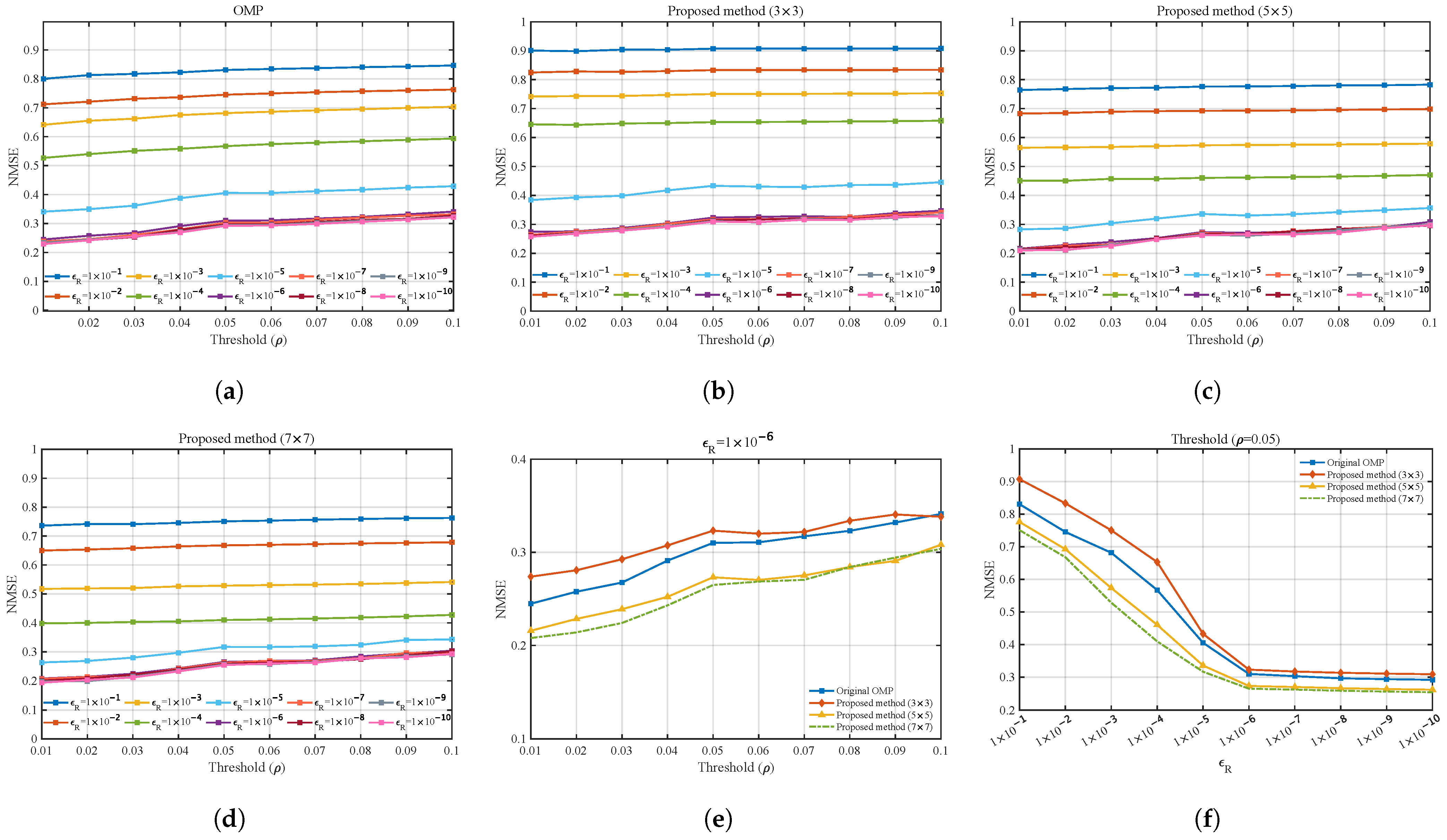
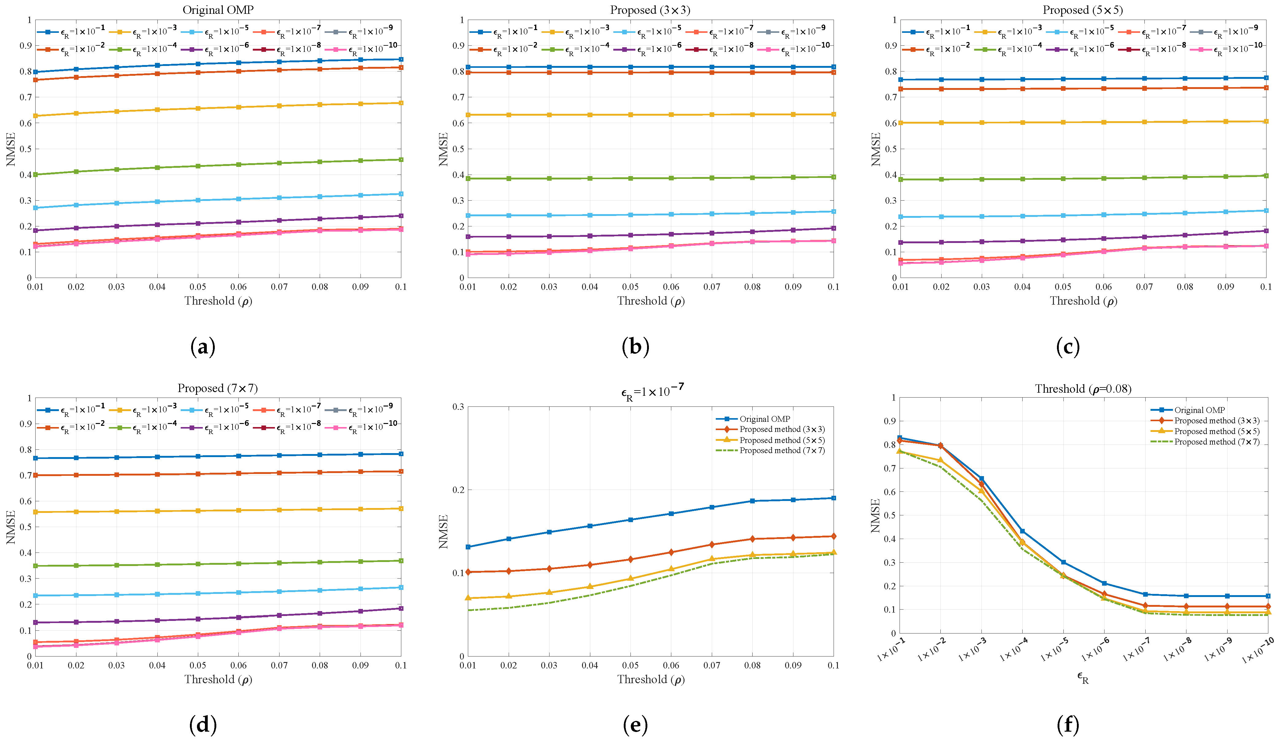
The iteration stopping criteria ${\epsilon }_R$ of the OMP algorithm, along with the activation threshold $\rho$, governs the trade-off between reconstruction fidelity and background clutter suppression. The smaller ${\epsilon }_R$ is, the smaller the difference between the reconstructed image and the original image, but the more background clutter is included in the reconstructed image. The larger $\rho$ is, the more background clutter is removed from the reconstructed image. In order to maximize the retention of target components in the reconstructed image and minimize the inclusion of background clutter, the parameters ${\epsilon }_R$ and $\rho$ are determined using all samples in the training set of the MSTAR dataset under SOC in Table 3 and all samples in the training set of the OpenSARShip dataset under six-class in Table 9, with optimization guided by the normalized mean square error (NMSE) defined as

$$\mathrm{NMSE}={\displaystyle \frac{1}{K}}{\displaystyle \sum _{k=1}^K}{\displaystyle \frac{{∥|{\tilde{I}}^k(x,y)|-{\hat{I}}_{\rho }^k(x,y)∥}_2^2}{{∥{\tilde{I}}^k(x,y)∥}_2^2}};$$

(18)

Here, ${\tilde{I}}^k(x,y)$ denotes the k-th original image, ${\hat{I}}_{\rho }^k(x,y)$ denotes its reconstructed image, and K denotes the total number of samples. Based on the experience in [28,31], the ranges of ${\epsilon }_R$ and $\rho$ are set to $[1\times {10}^{-10},1\times {10}^{-1}]$ and $[0.01,0.1]$, respectively. The bandwidth and other parameters are summarized in Table 2.

As shown in Figure 7a–d and Figure 8a–d, for the same $\rho$, the smaller ${\epsilon }_R$ leads to the reconstructed image being more similar to the original image, resulting in a smaller NMSE, but the smaller ${\epsilon }_R$ also means more background clutter is included; for the same ${\epsilon }_R$, the larger $\rho$ leads to more background clutter being removed from the reconstructed image, resulting in a larger NMSE, and the larger $\rho$ also makes it more likely to remove the target components while removing background clutter. Therefore, it is necessary to find ${\epsilon }_R$ and $\rho$ from different ranges such that the NMSE remains stable, ensuring the target component is reconstructed as completely as possible while background clutter is removed as much as possible. It can be seen from Figure 7a–d and Figure 8a–d, the NMSE remains stable under the parameter conditions ${\epsilon }_R\le 1\times {10}^{-6}$, $\rho \ge 0.05$ and ${\epsilon }_R\le 1\times {10}^{-7}$, $\rho \ge 0.08$, respectively.

To reduce the blocking artifacts, the OMP-IC uses overlapping blocks to crop the SAR images into image blocks of $3\times 3$ pixels, $5\times 5$ pixels, and $7\times 7$ pixels, respectively. The smaller the cropped image blocks, the smaller the overlapping area between image blocks, the more severe the blocking artifacts, and the worse the quality of the reconstructed image, resulting in a larger NMSE. As demonstrated in Figure 7e,f and Figure 8e,f, the NMSE of the OMP-IC algorithm is lower than that of the original OMP method when the block size exceeds $5\times 5$ pixels.

Table 10. Reconstruction capability comparison.

Algorithm	Memory Consumption (Bytes)		Computational Time (Seconds)
	MSTAR	OpenSARShip	MSTAR	OpenSARShip
Original OMP	$3.96\times {10}^9$	$1.85\times {10}^9$	$54.56$	$56.03$
proposed ($3\times 3$)	$9.58\times {10}^8$	$2.67\times {10}^8$	$12.72$	$13.17$
proposed ($5\times 5$)	$9.60\times {10}^8$	$2.69\times {10}^8$	$14.03$	$15.21$
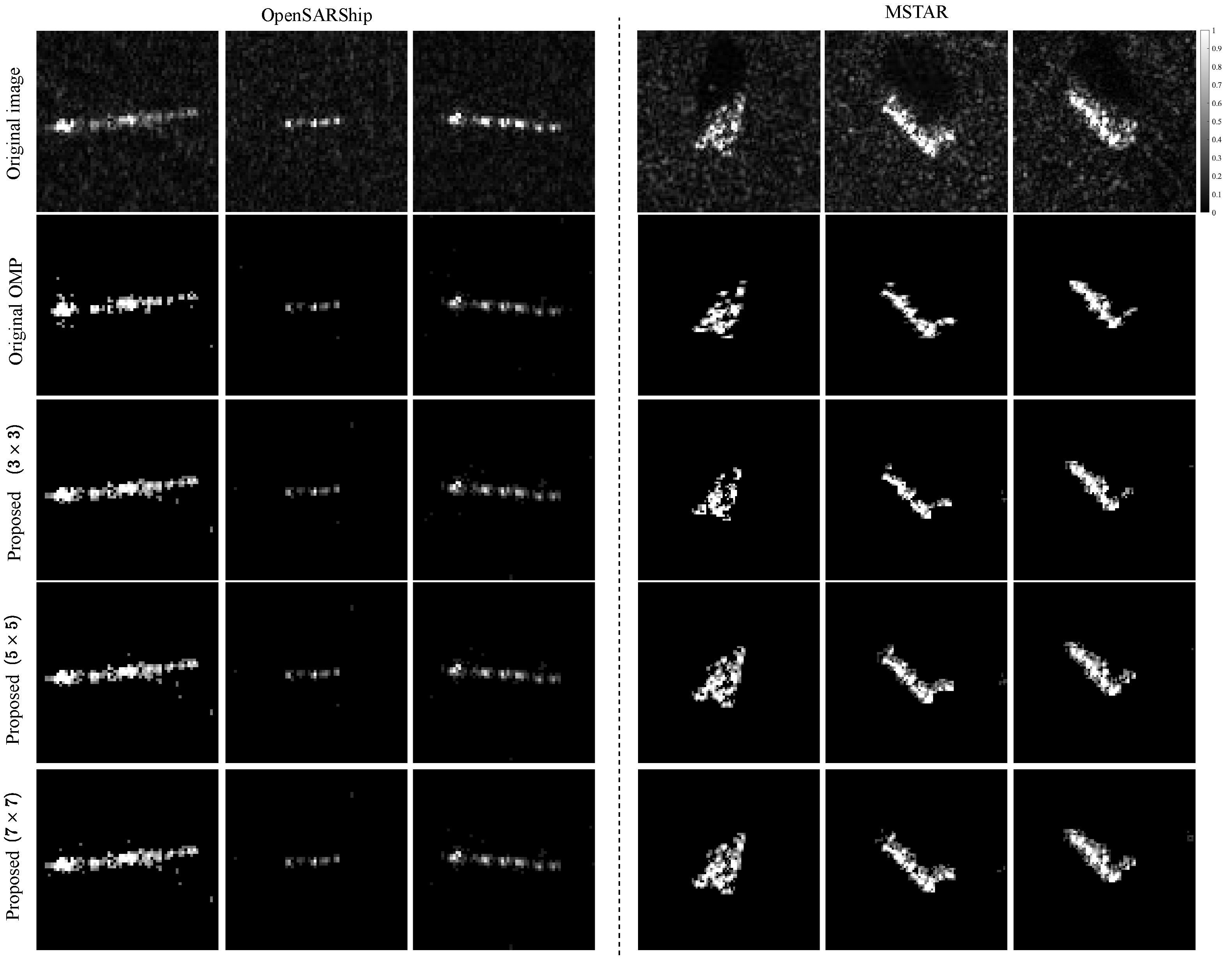
proposed ($7\times 7$)	$9.65\times {10}^8$	$2.73\times {10}^8$	$24.48$	$26.21$

compares the average memory consumption and computational time between the original OMP-based algorithm and the proposed OMP-IC algorithm, evaluated under the parameter sets ${\epsilon }_R=1\times {10}^{-6}$, $\rho =0.05$ for the MSTAR dataset and ${\epsilon }_R=1\times {10}^{-7}$, $\rho =0.08$ for the OpenSARShip dataset. As the block size in the OMP-IC increases, the stored dictionary and computational load for reconstruction increase accordingly, while the corresponding NMSE decreases. When the block size exceeds $5\times 5$ pixels, the computational speed of the OMP-IC algorithm nearly doubles. Based on a comprehensive evaluation of the NMSE, memory consumption, and computational efficiency, the parameters selected for OMP-IC reconstructions are ${\epsilon }_R=1\times {10}^{-6}$, $\rho =0.05$, and a block size of $5\times 5$ pixels for the MSTAR dataset, and ${\epsilon }_R=1\times {10}^{-7}$, $\rho =0.08$, with the same block size for the OpenSARShip dataset. Figure 9 presents the reconstruction results of different samples using each algorithm.

4.4. Comparison Experiment

4.4.1. Compared Methods

The compared methods are shown in

Table 11. The characteristics of compared methods.

Method	Input Image	Image Size	Pretrained
ResNet50 [6]	Amplitude	$88\times 88$	No
VGG16 [5]	Amplitude	$88\times 88$	No
AconvNets [7]	Amplitude	$88\times 88$	No
AM-CNN [8]	Amplitude	$100\times 100$	No
SNINet [20]	Amplitude	$88\times 88$	No
CFA-FVGGNet [21]	Amplitude	$88\times 88$	Yes
IRSC-RVGGNet [13]	Complex	$128\times 128$	Yes
MS-PHIA [28]	Complex	$64\times 64$	No
ERFA-FVGGNet	Complex	$88\times 88$	Yes

, ResNet50 [6] and VGG16 [5] are data-driven networks designed for optical image recognition, A-ConvNets [7] and AM-CNN [8] are data-driven networks designed for SAR target recognition, SNINet [20] and CFA-FVGGNet [21] are domain alignment and data-driven based SAR target recognition methods, and IRSC-RVGGNet [13] and MS-PIHA [28] are data-driven networks fusing ASCs. Specifically, CFA-FVGGNet combines the CFA method with the proposed FVGGNet for comparison with ERFA. To ensure the fairness, the reconstructed results obtained using the proposed OMP-IC are uniformly used as ASCs; all model parameters follow their original literature implementations; and no data augmentation techniques are applied during training.

4.4.2. Results of MSTAR SOC

The experimental results under SOC are presented in

Table 12. Performances of different methods under MSTAR SOC.

Framework	Method	${\mathbf{WCRS}}_{\mathbf{tg}}$ (%)	${\mathbf{WCRS}}_{\mathbf{sd}}$ (%)	${\mathbf{WCRS}}_{\mathbf{bg}}$ (%)	OA (%)
Optical-based	ResNet50 [6]	$36\pm 3$	$23\pm 3$	$\mathbf{41}\pm \mathbf{2}$	$97.18\pm 0.62$
	VGG16 [5]	$35\pm 4$	$22\pm 3$	$\mathbf{43}\pm \mathbf{3}$	$96.45\pm 1.24$
SAR-based	AconvNets [7]	$40\pm 3$	$18\pm 2$	$\mathbf{42}\pm \mathbf{3}$	$99.03\pm 0.10$
	AM-CNN [8]	$39\pm 4$	$21\pm 3$	$\mathbf{40}\pm \mathbf{3}$	$98.30\pm 0.68$
Domain align	SNINet [20]	$36\pm 1$	$26\pm 0$	$\mathbf{38}\pm \mathbf{1}$	$97.43\pm 0.32$
	CFA-FVGGNet [21]	$\mathbf{55}\pm \mathbf{2}$	$34\pm 2$	$11\pm 1$	$98.74\pm 0.21$
ASCs fusion	IRSC-RVGGNet [13]	$33\pm 1$	$28\pm 2$	$\mathbf{39}\pm \mathbf{1}$	$99.46\pm 0.10$
	MS-PHIA [28]	$\mathbf{53}\pm \mathbf{1}$	$19\pm 1$	$28\pm 1$	$99.36\pm 0.09$
ERFA	ERFA-FVGGNet	$\mathbf{76}\pm \mathbf{1}$	$13\pm 1$	$11\pm 1$	$\mathbf{99}.\mathbf{68}\pm \mathbf{0}.\mathbf{11}$

The bold in WCRS highlights the region with the dominant proportion in the decision-making basis and in OA highlights the best result. All results are the mean ± standard deviation across five repeated experiments.

, with WCRS evaluation conducted for each model. Given the minimal distribution differences between the training and test sets, all methods achieve accuracy rates exceeding 96%. However, in the two optical-based networks (ResNet50 and VGG16), background clutter dominated their decision-making basis, accounting for over $40\%$, which suggests overinterpretation. While the two SAR-based networks, A-ConvNets and AM-CNN, achieve accuracy rates exceeding 98%, yet background clutter similarly dominates their decision-making basis, indicating overinterpretation. Among the three domain alignment methods—SNINet, CFA-FVGGNet and ERFA-FVGGNet—recognition accuracy exceeds 97%. However, SNINet shows a lower recognition rate than the other two methods with overinterpretation. CFA-FVGGNet’s CWMSE contrastive loss improves decision-making basis focus on target and shadow regions while effectively avoiding overinterpretation, but its accuracy rate decreases compared to ERFA-FVGGNet, demonstrating that CWMSE induces excessive feature alignment that degrades recognition performance. The three ASC component-integrated methods—IRSC-RVGGNet, MS-PIHA and ERFA-FVGGNet—achieve recognition rates exceeding 99%, validating the strong discriminability of ASC components. However, IRSC-RVGGNet, which concatenates independent ASC component slices, partially loses ASC positioning information, leading to overinterpretation. Furthermore, ERFA-FVGGNet significantly concentrates decision-making on target regions, outperforming MS-PIHA’s attention mechanism and IRSC-RVGGNet’s feature concatenation. Both AM-CNN and MS-PIHA utilize attention mechanisms, but MS-PIHA enhances interpretability through ASC-activated physical attention, whereas AM-CNN’s unconstrained attention leads to background clutter overfitting and overinterpretation [19,47]. Experimental results under SOC validate that the proposed ERFA-FVGGNet superiorly mitigates model overinterpretation, improves interpretability, and enhances recognition performance.

4.4.3. Results of MSTAR EOC-Depression

As depression angles change, target signatures, shadow regions, and background clutter all undergo variations.

Table 13. Performances of different methods under MSTAR EOCs.

Framework	Method	OA (%)
		EOC-Depression	EOC-Version	EOC-Configuration	EOC-Scene
Optical-based	ResNet50 [6]	$74.25\pm 0.74$	$95.18\pm 0.68$	$96.03\pm 1.05$	$74.75\pm 2.04$
	VGG16 [5]	$74.39\pm 2.27$	$93.89\pm 2.32$	$95.79\pm 1.23$	$58.87\pm 1.50$
SAR-based	AconvNets [7]	$89.96\pm 0.57$	$96.18\pm 0.59$	$97.71\pm 0.60$	$67.75\pm 3.09$
	AM-CNN [8]	$85.12\pm 0.94$	$92.43\pm 3.00$	$94.62\pm 2.40$	$79.41\pm 2.13$
Domain align	SNINet [20]	$90.72\pm 0.11$	$95.27\pm 0.69$	$96.87\pm 1.10$	$72.44\pm 2.43$
	CFA-FVGGNet [21]	$93.55\pm 0.70$	$96.84\pm 2.21$	$96.41\pm 1.18$	$90.39\pm 2.15$
ASCs fusion	IRSC-RVGGNet [13]	$86.32\pm 2.02$	$96.81\pm 1.63$	$96.97\pm 1.39$	$81.75\pm 0.94$
	MS-PHIA [28]	$92.32\pm 0.34$	$98.12\pm 0.20$	$99.27\pm 0.28$	$91.92\pm 1.73$
ERFA	ERFA-FVGGNet	$\mathbf{97}.\mathbf{12}\pm \mathbf{0}.\mathbf{66}$	$\mathbf{99}.\mathbf{11}\pm \mathbf{0}.\mathbf{19}$	$\mathbf{99}.\mathbf{65}\pm \mathbf{0}.\mathbf{15}$	$\mathbf{95}.\mathbf{32}\pm \mathbf{0}.\mathbf{45}$

The bold highlights the best result. All results are the mean OA (%) ± standard deviation across five repeated experiments.

demonstrates model performances under depression angle variations. ResNet50, VGG16, A-ConvNets, and AM-CNN exhibit over a 9% accuracy rate drop compared to SOC, and background clutter constitutes the dominant portion of the decision-making basis. SNINet and IRSC-RVGGNet rely on background clutter as the primary basis for decisions and exhibit a reduction in accuracy to approximately 90%. To address the lack of image segmentation data under EOCs [48], reconstructed ASC components using OMP-IC are integrated into CFA-FVGGNet’s target domain data, reducing background clutter dependency and achieving over 93% recognition rate. MS-PIHA also surpasses the 92% accuracy rate by prioritizing target regions as the decision-making basis, demonstrating that focusing on target regions enhances model robustness under depression angle variations. The proposed ERFA-FVGGNet achieves a 97.12% recognition rate with the highest proportion of target regions within the decision-making basis, proving target region variations are smaller than background clutter changes under depression angle variations, while highlighting the robustness of ERFA-FVGGNet in depression variation.

4.4.4. Results of MSTAR EOC-Version

Although target version variations lead to changes in the target’s shape and contour, the resolution of only 0.3 m of SAR images means such variations have limited impact on models [47]. The recognition accuracy of all methods exceeds $92\%$, as summarized in Table 13. Notably, purely data-driven methods (ResNet50, VGG16, A-ConvNets, and AM-CNN) achieve accuracy rates above $92\%$, while domain alignment methods (SNINet, CFA-FVGGNet and ERFA-FVGGNet) surpass $95\%$, and ASCs fusion methods (IRSC-RVGGNet, MS-PIHA and ERFA-FVGGNet) reach beyond $96\%$. ERFA-FVGGNet achieves a $2.3\%$ higher accuracy rate than CFA-FVGGNet, indicating that CLIP contrastive loss outperforms CWMSE in model generalization.

4.4.5. Results of MSTAR EOC-Configuration

The impact of target configuration variants is similar to that of version variations. All models demonstrate recognition rates over $94\%$, as shown in Table 13, which induce small performance fluctuations, particularly MS-PIHA and the proposed ERFA-FVGGNet, showing less than a $0.1\%$ variation compared to SOC. Meanwhile, ERFA-FVGGNet achieves more than $1\%$ higher accuracy rate than other methods, demonstrating its superior generalization under configuration variations.

4.4.6. Results of MSTAR EOC-Scene

Scene transitions induce significant distributional shifts and characteristic alterations in background clutter. As shown in Table 13, six methods (ResNet50, VGG16, A-ConvNets, AM-CNN, SNINet, and IRSC-RVGGNet) relying primarily on background clutter as a decision-making basis exhibited accuracy rates below $80\%$, which demonstrates that overinterpretation severely degrades model robustness under background clutter variations. In contrast, three methods (CFA-FVGGNet, MS-PIHA, and ERFA-FVGGNet) prioritizing the target region maintained recognition rates above $90\%$. The proposed ERFA-FVGGNet achieves $95.32\%$ recognition accuracy by aligning electromagnetic features to emphasize target regions as a decision-making basis, proving its superior scene-transition robustness compared to other methods.

4.4.7. Results of MSTAR OFA

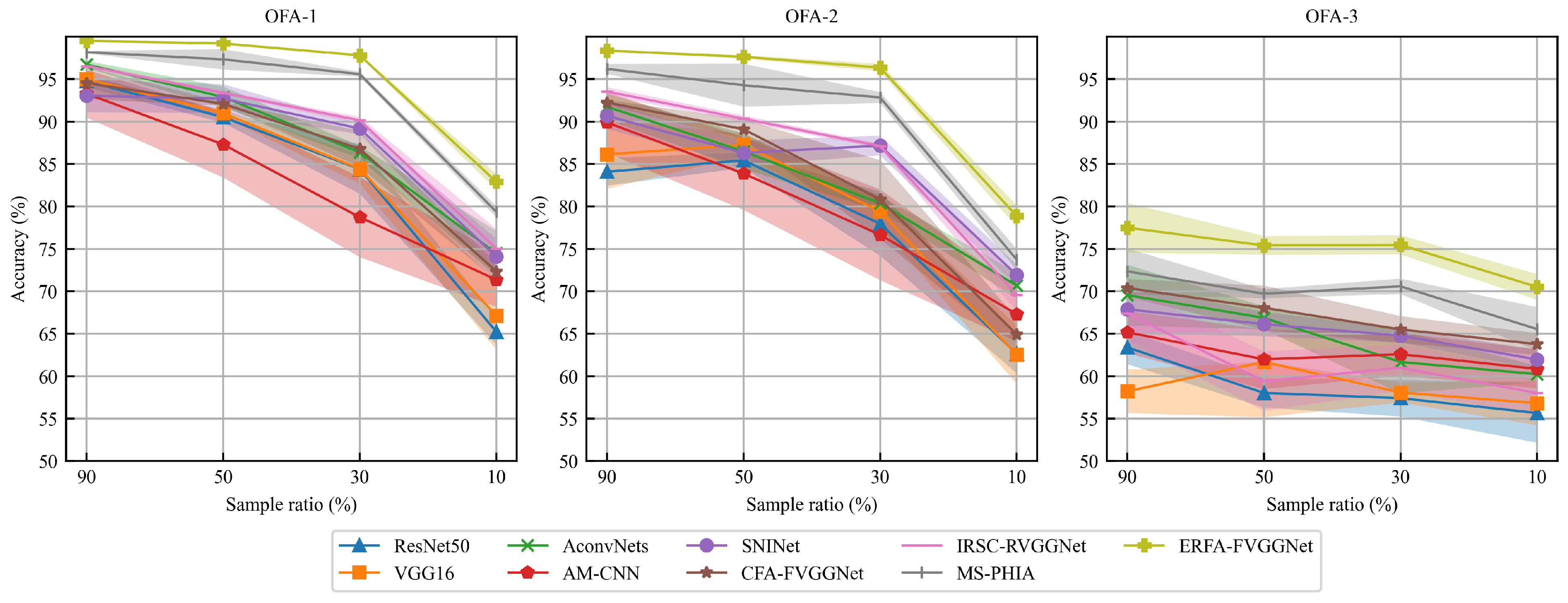
Randomly select 90%, 50%, 30%, and 10% samples of the training set to verify model robustness and generalization [28]. The corresponding results are presented in

Table 14. Performances of different methods under MSTAR OFA.

Method	90			50
	OFA-1	OFA-2	OFA-3	OFA-1	OFA-2	OFA-3
ResNet50 [6]	$94.75\pm 0.73$	$84.08\pm 1.63$	$63.38\pm 1.97$	$90.52\pm 0.67$	$85.43\pm 0.89$	$58.02\pm 1.73$
VGG16 [5]	$95.00\pm 0.30$	$86.13\pm 4.04$	$58.21\pm 2.57$	$90.99\pm 0.42$	$87.26\pm 1.32$	$58.42\pm 3.26$
AconvNets [7]	$96.71\pm 0.42$	$91.74\pm 1.51$	$69.55\pm 3.58$	$92.89\pm 1.24$	$86.48\pm 2.09$	$66.86\pm 1.36$
AM-CNN [8]	$93.28\pm 3.82$	$89.89\pm 3.59$	$65.17\pm 4.47$	$87.30\pm 3.89$	$83.88\pm 4.30$	$61.98\pm 3.52$
SNINet [20]	$93.03\pm 1.95$	$90.67\pm 1.55$	$67.87\pm 2.75$	$92.70\pm 1.70$	$86.30\pm 1.48$	$66.12\pm 1.43$
CFA-FVGGNet [21]	$94.53\pm 1.90$	$92.24\pm 0.30$	$70.38\pm 1.06$	$92.08\pm 0.22$	$89.09\pm 1.19$	$68.05\pm 2.62$
IRSC-RVGGNet [13]	$96.54\pm 0.33$	$93.53\pm 0.50$	$67.39\pm 3.17$	$93.38\pm 0.17$	$90.33\pm 0.38$	$59.41\pm 3.50$
MS-PHIA [28]	$98.17\pm 0.15$	$96.20\pm 0.57$	$72.34\pm 2.71$	$97.32\pm 1.20$	$94.28\pm 2.53$	$69.71\pm 0.54$
ERFA-FVGGNet	$\mathbf{99.51}\pm \mathbf{0.08}$	$\mathbf{98.36}\pm \mathbf{0.13}$	$\mathbf{77.49}\pm \mathbf{2.92}$	$\mathbf{99.20}\pm \mathbf{0.08}$	$\mathbf{97.62}\pm \mathbf{0.19}$	$\mathbf{75.40}\pm \mathbf{1.11}$
Method	30			10
	OFA-1	OFA-2	OFA-3	OFA-1	OFA-2	OFA-3
ResNet50 [6]	$84.40\pm 2.91$	$77.96\pm 3.78$	$57.40\pm 2.16$	$65.23\pm 1.54$	$62.63\pm 2.29$	$55.65\pm 3.51$
VGG16 [5]	$84.43\pm 1.76$	$79.39\pm 1.76$	$58.07\pm 1.18$	$67.13\pm 4.01$	$62.53\pm 3.45$	$56.80\pm 2.58$
AconvNets [7]	$86.36\pm 0.75$	$80.37\pm 0.85$	$61.67\pm 3.71$	$74.47\pm 2.64$	$70.67\pm 1.53$	$60.23\pm 0.98$
AM-CNN [8]	$78.73\pm 4.71$	$76.65\pm 5.34$	$62.58\pm 2.51$	$71.36\pm 3.21$	$67.31\pm 3.23$	$60.85\pm 3.30$
SNINet [20]	$89.17\pm 0.65$	$87.16\pm 1.16$	$64.77\pm 0.83$	$74.08\pm 2.09$	$71.90\pm 1.25$	$61.96\pm 1.15$
CFA-FVGGNet [21]	$86.78\pm 2.14$	$80.82\pm 4.62$	$65.50\pm 1.58$	$72.33\pm 1.04$	$64.91\pm 1.92$	$63.77\pm 1.29$
IRSC-RVGGNet [13]	$90.14\pm 0.42$	$87.11\pm 0.28$	$60.98\pm 2.74$	$75.02\pm 2.33$	$69.58\pm 1.98$	$58.01\pm 2.72$
MS-PHIA [28]	$95.58\pm 0.29$	$92.83\pm 0.64$	$70.58\pm 0.91$	$79.36\pm 0.66$	$73.73\pm 1.26$	$65.54\pm 2.59$
ERFA-FVGGNet	$\mathbf{97.80}\pm \mathbf{0.14}$	$\mathbf{96.36}\pm \mathbf{0.44}$	$\mathbf{75.47}\pm \mathbf{1.13}$	$\mathbf{82.90}\pm \mathbf{0.95}$	$\mathbf{78.86}\pm \mathbf{1.28}$	$\mathbf{70.51}\pm \mathbf{1.51}$

The $\mathbf{bold}$ highlights the best result. All results are the mean OA (%) ± standard deviation across five repeated experiments.

and Figure 10, all evaluated models exhibit lower accuracy rates compared to their performance under SOCs and EOCs, indicating that OFA imposes a stricter evaluation protocol, thereby enhancing task challenge. ERFA-FVGGNet achieves the best performance across all twelve experiments. In the most challenging OFA-3 using 10% training samples, ERFA-FVGGNet outperforms the second-best result by 4.97%.

OFA-1 evaluation shares identical target versions/configurations, scene and similar depression angles between training and test sets and is used to test model generalization under sample missing conditions. As shown in Table 14, the recognition rates decrease as the proportion of training samples reduces; ERFA-FVGGNet exceeds the second-best result by more than 1% under all sample ratios. In contrast, the four purely data-driven methods (ResNet50, VGG16, A-ConvNets, and AM-CNN) exhibit recognition rates below 90% when training samples account for less than 50%, indicating weak generalization. Among domain alignment methods, CFA-FVGGNet’s CWMSE contrastive loss led to excessive feature alignment and limited generalization, while SNINet’s speckle noise suppression provided limited improvement. ASCs-based methods (IRSC-RVGGNet, MS-PIHA, ERFA-FVGGNet) outperformed others, demonstrating that electromagnetic reconstruction features can enhance model recognition performance under limited samples. Among these, ERFA-FVGGNet maximizes the advantages of reconstructed features, achieving superior generalization in OFA-1.

OFA-2 introduces BMP2 version variants and T72 version/configuration variants to the test set, enabling a comprehensive evaluation of model generalization under limited samples and target version/configuration changes. As shown in Table 14, all models show over 1% accuracy drops compared to OFA-1 but maintain similar trends across sample ratios. ERFA-FVGGNet consistently outperforms the second-best method by over 2% across all sample ratios, proving superior generalization against version/configuration variations.

OFA-3 represents the most challenging scenario using 2S1/BRDM2/ZSU234 with varying depression angles and scenes, aiming to evaluate model robustness under observation angle and scene changes. As shown in Table 14, the recognition performance of all methods under OFA-3 decreases significantly compared to OFA-1 and OFA-2. Target-region-focused methods (CFA-FVGGNet, MS-PIHA, ERFA-FVGGNet) demonstrated stronger robustness by suppressing overinterpretation, indicating that target region features possess greater stability and distinguishability under observation angle and scene variations. ERFA-FVGGNet outperforms MS-PIHA by more than 4.89% and by CFA-FVGGNet over 6.74% across all sample ratios, demonstrating its superior robustness under depression/scene variations. The excellent performance of the proposed ERFA-FVGGNet across OFA fully validates that ERFA has the ability to enhance model robustness, generalization, and interpretability.

4.4.8. Results of OpenSARShip Three-Class and Six-Class

The experimental results for the OpenSARShip dataset under both three-class and six-class are summarized in

Table 15. Performances of different methods under OpenSARShip three-class and six-class.

Method	Three-Class			Six-Class
	${\mathbf{WCRS}}_{\mathbf{tg}}$ (%)	${\mathbf{WCRS}}_{\mathbf{bg}}$ (%)	OA (%)	${\mathbf{WCRS}}_{\mathbf{tg}}$ (%)	${\mathbf{WCRS}}_{\mathbf{bg}}$ (%)	OA (%)
ResNet50 [6]	$45\pm 5$	$\mathbf{55}\pm \mathbf{5}$	$78.81\pm 0.46$	$49\pm 4$	$\mathbf{51}\pm \mathbf{4}$	$52.74\pm 0.26$
VGG16 [5]	$\mathbf{54}\pm \mathbf{3}$	$46\pm 3$	$80.23\pm 1.32$	$41\pm 2$	$\mathbf{59}\pm \mathbf{2}$	$58.89\pm 0.50$
A-ConvNets [7]	$\mathbf{57}\pm \mathbf{3}$	$43\pm 3$	$81.00\pm 0.44$	$44\pm 3$	$\mathbf{56}\pm \mathbf{3}$	$57.51\pm 0.79$
AM-CNN [8]	$30\pm 8$	$\mathbf{70}\pm \mathbf{8}$	$82.03\pm 0.98$	$41\pm 4$	$\mathbf{59}\pm \mathbf{4}$	$57.11\pm 0.97$
SNINet [20]	$49\pm 2$	$\mathbf{51}\pm \mathbf{2}$	$81.00\pm 0.46$	$41\pm 3$	$\mathbf{59}\pm \mathbf{3}$	$55.92\pm 0.63$
CFA-FVGGNet [21]	$\mathbf{70}\pm \mathbf{3}$	$30\pm 3$	$82.45\pm 0.71$	$\mathbf{61}\pm \mathbf{1}$	$39\pm 1$	$59.06\pm 0.53$
IRSC-RVGGNet [13]	$40\pm 2$	$\mathbf{60}\pm \mathbf{2}$	$82.87\pm 0.31$	$29\pm 2$	$\mathbf{72}\pm \mathbf{2}$	$58.00\pm 0.43$
MS-PHIA [28]	$49\pm 2$	$\mathbf{51}\pm \mathbf{2}$	$82.49\pm 0.82$	$45\pm 2$	$\mathbf{55}\pm \mathbf{2}$	$58.75\pm 0.81$
ERFA-FVGGNet	$\mathbf{68}\pm \mathbf{2}$	$32\pm 2$	$\mathbf{85.74}\pm \mathbf{0.29}$	$\mathbf{60}\pm \mathbf{2}$	$40\pm 2$	$\mathbf{62.11}\pm \mathbf{0.63}$

The $\mathbf{bold}$ in WCRS highlights the region with the dominant proportion in the decision-making basis and in OA highlights the best result. All results are the mean ± standard deviation across five repeated experiments.

. Due to the complex operating conditions inherent in maritime SAR imagery, all methods achieve accuracy below 90%. In the three-class experiments, the decision-making basis of ResNet50, AM-CNN, SNINet, IRSC-RVGGNet and MS-PIHA is predominantly influenced by background clutter, accounting for over 50%, which indicates a tendency toward overinterpretation. In contrast, models including VGG16, A-ConvNets, CFA-FVGGNet and the proposed ERFA-FVGGNet rely more substantially on target regions. Notably, CFA-FVGGNet and ERFA-FVGGNet achieve notably higher target region contributions of approximately 70% with a recognition accuracy exceeding 82%. Among the three methods that utilize ASC components—IRSC-RVGGNet, MS-PIHA, and ERFA-FVGGNet—all attain recognition rates above 82%. However, IRSC-RVGGNet and MS-PIHA exhibit overinterpretation due to interference from complex maritime background clutter. In comparison, ERFA-FVGGNet achieves an overall accuracy of 85.74% and concentrates its decision-making basis on target regions.

In the six-class classification experiments, the performance of all models is consistently lower than that in the three-class. This decline can be attributed to the significant class imbalance issue, particularly the limited number of samples for fishing and general cargo compared to other ship types, which adversely affects the classification results. Moreover, with the exception of CFA-FVGGNet and the proposed ERFA-FVGGNet, all models exhibit a decision-making basis dominated by background clutter, indicating a tendency toward overinterpretation. Detailed results show that in the six-class experiment, none of the models achieve an accuracy exceeding $60\%$, except for ERFA-FVGGNet, which outperforms the second-best model, CFA-FVGGNet, by a margin of $3.05\%$. Experiments conducted on the OpenSARShip dataset under both three-class and six-class settings validate that the proposed ERFA improves overall recognition performance and effectively mitigates model overinterpretation and enhances interpretability and generalization.

4.5. Ablation Experiments

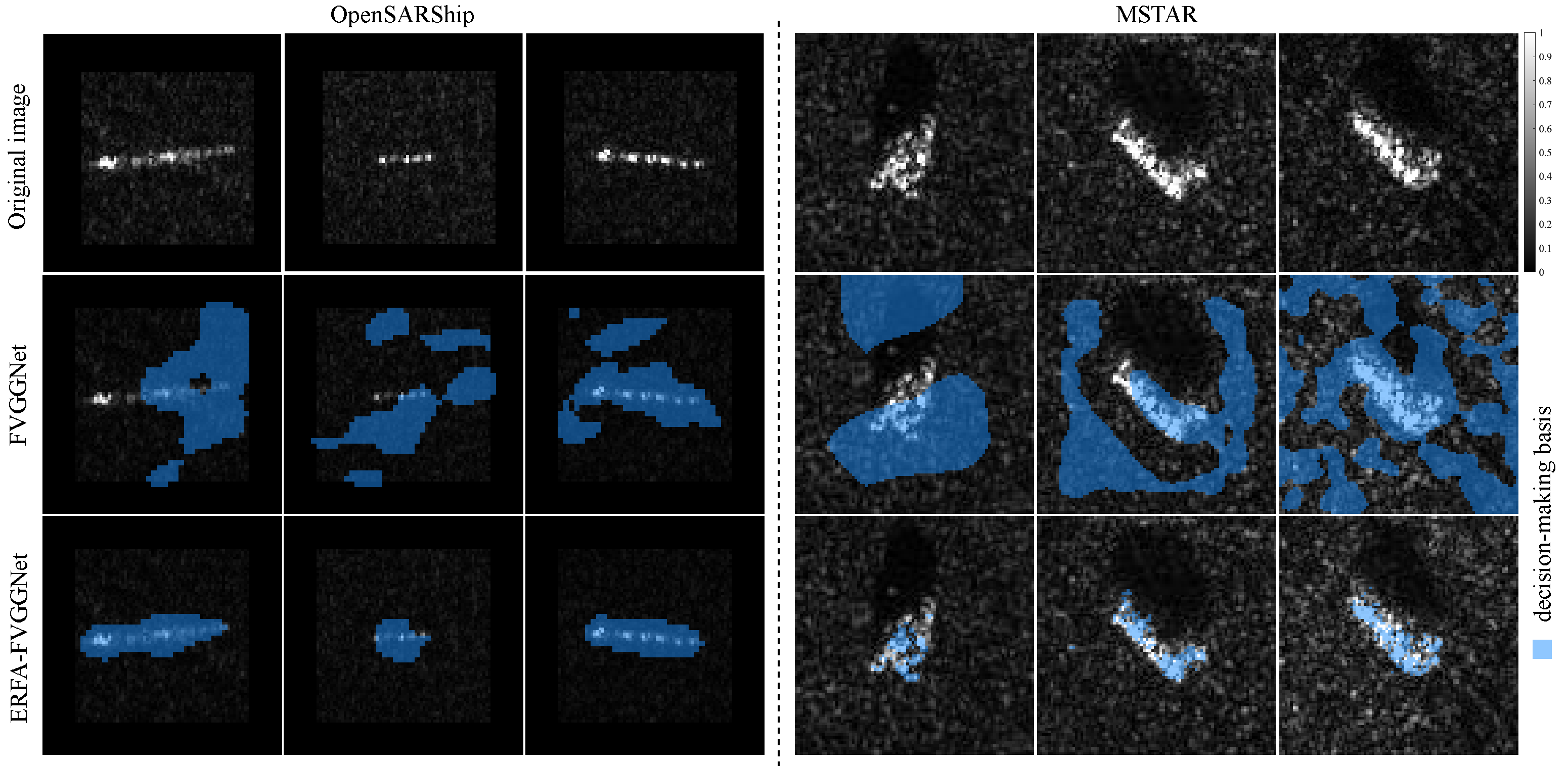
To validate the contribution of each module in the proposed method to recognition performance and background clutter suppression, we employ a non-pretrained FVGGNet as the baseline under the MSTAR SOC and OpenSARShip six-class. Experimental results in

Table 16. Ablation experiments under MSTAR SOC.

Method	ERFA		Pretrained	${\mathbf{WCRS}}_{\mathbf{tg}}$ (%)	${\mathbf{WCRS}}_{\mathbf{sd}}$ (%)	${\mathbf{WCRS}}_{\mathbf{bg}}$ (%)	OA (%)
	Original OMP	OMP-IC
FVGGNet				$35\pm 4$	$22\pm 3$	$\mathbf{43}\pm \mathbf{3}$	$97.18\pm 0.62$
	✓			$\mathbf{76}\pm \mathbf{1}$	$13\pm 1$	$11\pm 1$	$97.76\pm 0.67$
		✓		$\mathbf{75}\pm \mathbf{2}$	$12\pm 1$	$13\pm 1$	$98.19\pm 0.11$
			✓	$37\pm 1$	$21\pm 1$	$\mathbf{42}\pm \mathbf{1}$	$99.24\pm 0.28$
	✓		✓	$\mathbf{76}\pm \mathbf{1}$	$11\pm 1$	$13\pm 1$	$99.58\pm 0.05$
		✓	✓	$\mathbf{76}\pm \mathbf{1}$	$13\pm 1$	$11\pm 1$	$\mathbf{99.68}\pm \mathbf{0.11}$

The $\mathbf{bold}$ in WCRS highlights the region with the dominant proportion in the decision-making basis, and in OA highlights the best result. All results are the mean ± standard deviation across five repeated experiments.

demonstrate that the baseline achieves a recognition rate of 97.18% on MSTAR SOC, yet exhibits over 40% background clutter proportion in its decision-making basis, indicating overinterpretation. After integrating the ERFA module, the non-pretrained FVGGNet increases target region proportion to 75% and improves recognition accuracy by over 1%, confirming ERFA’s capacity to suppress clutter and enhance recognition. Although the introduction of ImageNet-pretrained weights to FVGGNet increases the baseline recognition rate by more than 2%, demonstrating the benefit of pretraining for recognition performance, background clutter remains above 40%, still reflecting overinterpretation. The proposed ERFA-FVGGNet, which incorporates ERFA into the pretrained FVGGNet, surpasses the baseline by 2.5% recognition improvement and raises the target region proportion to over 75% in the decision-making basis, affirming its dual role in mitigating overinterpretation and boosting recognition. Notably, the enhanced recognition performance achieved by the OMP-IC algorithm, in contrast to the original OMP algorithm within the ERFA framework, can be directly linked to its reduced NMSE. This lower error metric signifies a higher-quality electromagnetic reconstruction, which is critical for the subsequent feature alignment step and ultimately bolsters the overall efficacy of the framework. The experimental results from the OpenSARShip dataset (

Table 17. Ablation experiments under OpenSARShip six-class.

Method	ERFA		Pretrained	${\mathbf{WCRS}}_{\mathbf{tg}}$ (%)	${\mathbf{WCRS}}_{\mathbf{bg}}$ (%)	OA (%)
	Original OMP	OMP-IC
FVGGNet				$33\pm 3$	$\mathbf{67}\pm \mathbf{3}$	$58.68\pm 0.86$
	✓			$\mathbf{56}\pm \mathbf{2}$	$44\pm 2$	$60.09\pm 0.53$
		✓		$\mathbf{58}\pm \mathbf{1}$	$42\pm 1$	$60.43\pm 0.37$
			✓	$42\pm 2$	$\mathbf{58}\pm \mathbf{2}$	$61.26\pm 0.17$
	✓		✓	$\mathbf{60}\pm \mathbf{1}$	$40\pm 1$	$61.42\pm 0.44$
		✓	✓	$\mathbf{60}\pm \mathbf{2}$	$40\pm 2$	$\mathbf{62.11}\pm \mathbf{0.63}$

The bold in WCRS highlights the region with the dominant proportion in the decision-making basis, and in OA highlights the best result. All results are the mean ± standard deviation across five repeated experiments.

) confirm that the proposed method follows a performance trend similar to the MSTAR SOC, underscoring the integrated contribution of all ERFA-FVGGNet modules to its recognition accuracy. As visually compared in Figure 11, the decision-making basis of ERFA-FVGGNet shows reduced background clutter dominance and improved focus on target regions compared to the baseline FVGGNet. Ablation studies further verify that ERFA plays a critical role in suppressing background clutter and enhancing target features.

5. Conclusions

This study introduces ERFA-FVGGNet, a novel method for trustworthy SAR ATR. The methodology integrates three key innovations: OMP-IC for efficient and precise electromagnetic reconstruction, FVGGNet to strengthen feature extraction and generalization capabilities, and dual-loss to suppress background clutter while enhancing robustness and interpretability. Comprehensive experiments across MSTAR and OpenSARShip datasets validate the proposed method’s superiority in robustness, generalization, and interpretability. Notably, our analysis demonstrates that the decision-making basis focus on target regions directly correlates with boosted trustworthiness. Future research will systematically investigate the latent potential of trustworthy target features in SAR ATR.

References

1. Zhang, T.; Jiang, L.; Xiang, D.; Ban, Y.; Pei, L.; Xiong, H. Ship detection from PolSAR imagery using the ambiguity removal polarimetric notch filter. ISPRS J. Photogramm. Remote Sens. 2019, 157, 41–58. [Google Scholar] [CrossRef]
2. Zhang, T.; Ji, J.; Li, X.; Yu, W.; Xiong, H. Ship detection from PolSAR imagery using the complete polarimetric covariance difference matrix. IEEE Trans. Geosci. Remote Sens. 2019, 57, 2824–2839. [Google Scholar] [CrossRef]
3. Zhang, T.; Yang, Z.; Xiong, H. PolSAR ship detection based on the polarimetric covariance difference matrix. IEEE J. Sel. Top. Appl. Earth Obs. Remote Sens. 2017, 10, 3348–3359. [Google Scholar] [CrossRef]
4. Zhang, T.; Xie, N.; Quan, S.; Wang, W.; Wei, F.; Yu, W. Polarimeric SAR Ship Detection based on the Sub-look Decomposition Technology. IEEE Trans. Radar Systems 2025, 1–15. [Google Scholar] [CrossRef]
5. Simonyan, K.; Zisserman, A. Very deep convolutional networks for large-scale image recognition. In Proceedings of the International Conference on Learning Representations, San Diego, CA, USA, 7–9 May 2015; pp. 1–14. [Google Scholar]
6. He, K.; Zhang, X.; Ren, S.; Sun, J. Deep residual learning for image recognition. In Proceedings of the 2016 IEEE Conference on Computer Vision and Pattern Recognition, Las Vegas, NV, USA, 27–30 June 2016; pp. 770–778. [Google Scholar]
7. Chen, S.; Wang, H.; Xu, F.; Jin, Y. Target classification using the deep convolutional networks for SAR images. IEEE Trans. Geosci. Remote Sens. 2016, 54, 4806–4817. [Google Scholar] [CrossRef]
8. Zhang, M.; An, J.; Yu, D.H.; Yang, L.D.; Wu, L.; Lu, X.Q. Convolutional neural network with attention mechanism for SAR automatic target recognition. IEEE Geosci. Remote Sens. Lett. 2022, 19, 4004205. [Google Scholar]
9. Huang, Z.; Pan, Z.; Lei, B. Transfer learning with deep convolutional neural network for SAR target classification with limited labeled data. Remote Sens. 2017, 9, 907. [Google Scholar] [CrossRef]
10. Huang, Z.; Pan, Z.; Lei, B. What, where, and how to transfer in SAR target recognition based on deep CNNs. IEEE Trans. Geosci. Remote Sens. 2020, 58, 2324–2336. [Google Scholar] [CrossRef]
11. Li, W.; Yang, W.; Liu, Y.; Li, X. Research and exploration on the interpretability of deep learning model in radar image. Sci. Sin. Inform. 2022, 52, 1114–1134. [Google Scholar] [CrossRef]
12. Deng, J.; Dong, W.; Socher, R.; Li, L.; Li, K.; Li, F. Imagenet: A large-scale hierarchical image database. In Proceedings of the 2009 IEEE Conference on Computer Vision and Pattern Recognition, Miami, FL, USA, 20–25 June 2009; pp. 248–255. [Google Scholar]
13. Zhang, J.; Xing, M.; Sun, G.; Bao, Z. Integrating the reconstructed scattering center feature maps with deep CNN feature maps for automatic SAR target recognition. IEEE Geosci. Remote Sens. Lett. 2022, 19, 4009605. [Google Scholar] [CrossRef]
14. Zhang, J.; Xing, M.; Xie, Y. FEC: A feature fusion framework for SAR target recognition based on electromagnetic scattering features and deep CNN features. IEEE Trans. Geosci. Remote Sens. 2021, 59, 2174–2187. [Google Scholar]
15. Yu, W. Automatic target recognition from an engineering perspective. J. Radars 2022, 11, 737–755. [Google Scholar]
16. Guo, W.; Zhang, Z.; Yu, W.; Sun, X. Perspective on explainable SAR target recognition. J. Radars 2020, 9, 462. [Google Scholar]
17. Li, W.; Yang, W.; Liu, L.; Zhang, W.; Liu, Y. Discovering and explaining the noncausality of deep learning in SAR ATR. IEEE Geosci. Remote Sens. Lett. 2023, 20, 4004605. [Google Scholar]
18. Cui, Z.; Yang, Z.; Zhou, Z.; Mou, L.; Tang, K.; Cao, Z.; Yang, J. Deep neural network explainability enhancement via causality-erasing SHAP method for SAR target recognition. IEEE Trans. Geosci. Remote Sens. 2024, 62, 5213415. [Google Scholar] [CrossRef]
19. Gao, Y.; Guo, W.; Li, D.; Yu, W. Can we trust deep learning models in SAR ATR? IEEE Geosci. Remote Sens. Lett. 2024, 21, 1–5. [Google Scholar]
20. Kwak, Y.; Song, W.J.; Kim, S.E. Speckle-noise-invariant convolutional neural network for SAR target recognition. IEEE Geosci. Remote Sens. Lett. 2019, 16, 549–553. [Google Scholar] [CrossRef]
21. Peng, B.; Xie, J.; Peng, B.; Liu, L. Learning invariant representation via contrastive feature alignment for clutter robust SAR ATR. IEEE Geosci. Remote Sens. Lett. 2023, 20, 4014805. [Google Scholar] [CrossRef]
22. Wang, J.; Quan, S.; Xing, S.; Li, Y.; Wu, H.; Meng, W. PSO-based fine polarimetric decomposition for ship scattering characterization. ISPRS J. Photogramm. Remote Sens. 2025, 220, 18–31. [Google Scholar]
23. Deng, J.; Wang, W.; Zhang, H.; Zhang, T.; Zhang, J. PolSAR ship detection based on superpixel-level contrast enhancement. IEEE Geosci. Remote Sens. Lett. 2024, 21, 4008805. [Google Scholar] [CrossRef]
24. Huang, B.; Zhang, T.; Quan, S.; Wang, W.; Guo, W.; Zhang, Z. Scattering enhancement and feature fusion network for aircraft detection in SAR images. IEEE Trans. Circuits Syst. Video Technol. 2025, 35, 1936–1950. [Google Scholar] [CrossRef]
25. Zeng, Z.; Sun, J.; Han, Z.; Hong, W. SAR automatic target recognition method based on multi-stream complex-valued networks. IEEE Trans. Geosci. Remote Sens. 2022, 60, 5228618. [Google Scholar] [CrossRef]
26. Zhang, H.; Wang, W.; Deng, J.; Guo, Y.; Liu, S.; Zhang, J. MASFF-Net: Multiazimuth scattering feature fusion network for SAR target recognition. IEEE J. Sel. Top. Appl. Earth Obs. Remote Sens. 2025, 18, 19425–19440. [Google Scholar] [CrossRef]
27. Liao, L.; Du, L.; Chen, J.; Cao, Z.; Zhou, K. EMI-Net: Sn end-to-end mechanism-driven interpretable network for SAR target recognition under EOCs. IEEE Trans. Geosci. Remote Sens. 2024, 62, 5205118. [Google Scholar] [CrossRef]
28. Huang, Z.; Wu, C.; Han, H.J. Physics inspired hybrid attention for SAR target recognition. ISPRS J. Photogramm. Remote Sens. 2024, 207, 164–174. [Google Scholar] [CrossRef]
29. Gerry, M.; Potter, L.; Gupta, I.; Van Der Merwe, A. A parametric model for synthetic aperture radar measurements. IEEE Trans. Antennas Propag. 1999, 47, 1179–1188. [Google Scholar] [CrossRef]
30. Koets, M.; Moses, R. Image domain feature extraction from synthetic aperture imagery. In Proceedings of the 1999 IEEE International Conference on Acoustics, Speech, and Signal Processing. Proceedings, Phoenix, AZ, USA, 15–19 March 1999; Volume 4, pp. 2319–2322. [Google Scholar]
31. Liu, H.; Jiu, B.; Li, F.; Wang, Y. Attributed scattering center extraction algorithm based on sparse representation with dictionary refinement. IEEE Trans. Antennas Propag. 2017, 65, 2604–2614. [Google Scholar] [CrossRef]
32. Fei, L.; Yanbing, L. Sparse based attributed scattering center extraction algorithm with dictionary refinement. In Proceedings of the 2016 CIE International Conference on Radar (RADAR), London, UK, 5–7 October 2016; pp. 1–4. [Google Scholar]
33. Radford, A.; Kim, J.W.; Hallacy, C.; Ramesh, A.; Goh, G.; Agarwal, S.; Sastry, G.; Askell, A.; Mishkin, P.; Clark, J.; et al. Learning transferable visual models from natural language supervision. In Proceedings of the 38th International Conference on Machine Learning, Online, 18–24 July 2021; Volume 139, pp. 8748–8763. [Google Scholar]
34. Xie, N.; Zhang, T.; Zhang, L.; Chen, J.; Wei, F.; Yu, W. VLF-SAR: A Novel Vision-Language Framework for Few-shot SAR Target Recognition. IEEE Trans. Circuits Syst. Video Technol. 2025, 35, 9530–9544. [Google Scholar] [CrossRef]
35. Duan, J.; Zhang, L.; Hua, Y. Modified ADMM-net for attributed scattering center decomposition of synthetic aperture radar targets. IEEE Geosci. Remote Sens. Lett. 2023, 20, 4014605. [Google Scholar] [CrossRef]
36. Ding, B.; Wen, G.; Ma, C.; Yang, X. An efficient and robust framework for SAR target recognition by hierarchically fusing global and local features. IEEE Trans. Image Process. 2018, 27, 5983–5995. [Google Scholar] [CrossRef]
37. Gan, L. Block compressed sensing of natural images. In Proceedings of the 2007 15th International Conference on Digital Signal Processing, Cardiff, UK, 1–4 July 2007; pp. 403–406. [Google Scholar]
38. Zhou, Y.; Guo, H. Collaborative block compressed sensing reconstruction with dual-domain sparse representation. Inf. Sci. 2019, 472, 77–93. [Google Scholar] [CrossRef]
39. Yang, D.; Ni, W.; Du, L.; Liu, H.; Wang, J. Efficient attributed scatter center extraction based on image-domain sparse representation. IEEE Trans. Signal Process. 2020, 68, 4368–4381. [Google Scholar] [CrossRef]
40. Zhu, X.; Tuia, D.; Mou, L.; Xia, G.; Zhang, L.; Xu, F.; Fraundorfer, F. Deep learning in remote sensing: A comprehensive review and list of resources. IEEE Geosci. Remote Sens. Mag. 2017, 5, 8–36. [Google Scholar] [CrossRef]
41. Zeiler, M.D.; Fergus, R. Visualizing and understanding convolutional networks. In Proceedings of the European Conference on Computer Vision, Zurich, Switzerland, 6–12 September 2014; pp. 818–833. [Google Scholar]
42. Wang, F.; Liu, H. Understanding the behaviour of contrastive loss. In Proceedings of the 2021 IEEE/CVF Conference on Computer Vision and Pattern Recognition, Nashville, TN, USA, 19–25 June 2021; pp. 2495–2504. [Google Scholar]
43. AFRL; DARPA. The Air Force Moving and Stationary Target Recognition Database. Available online: https://www.sdms.afrl.af.mil/datasets/mstar/ (accessed on 16 August 2025).
44. Huang, L.; Liu, B.; Li, B.; Guo, W.; Yu, W.; Zhang, Z.; Yu, W. OpenSARShip: A dataset dedicated to Sentinel-1 ship interpretation. IEEE J. Sel. Top. Appl. Earth Obs. Remote Sens. 2018, 11, 195–208. [Google Scholar] [CrossRef]
45. Li, B.; Liu, B.; Huang, L.; Guo, W.; Zhang, Z.; Yu, W. OpenSARShip 2.0: A large-volume dataset for deeper interpretation of ship targets in Sentinel-1 imagery. In Proceedings of the 2017 SAR in Big Data Era: Models, Methods and Applications, Beijing, China, 13–14 November 2017; pp. 1–5. [Google Scholar]
46. Ruder, S. An Overview of Gradient Descent Optimization Algorithms. 2016. Available online: https://arxiv.org/abs/1609.04747 (accessed on 16 August 2025).
47. Li, W.; Yang, W.; Zhang, W.; Liu, T.; Liu, Y.; Liu, L. Hierarchical disentanglement-alignment network for robust SAR vehicle recognition. IEEE J. Sel. Top. Appl. Earth Obs. Remote Sens. 2023, 16, 9661–9679. [Google Scholar] [CrossRef]
48. Malmgren-Hansen, D.; Nobel-Jorgensen, M. Convolutional neural networks for SAR image segmentation. In Proceedings of the 2015 IEEE International Symposium on Signal Processing and Information Technology, Abu Dhabi, United Arab Emirates, 7–10 December 2015; pp. 231–236. [Google Scholar]
49. Otsu, N. A threshold selection method from gray-level histograms. IEEE Trans. Syst. Man Cybern. 1979, 9, 62–66. [Google Scholar] [CrossRef]
Figure 1. SAR images of the same target under different operating conditions.
Remotesensing 17 03855 g001
Figure 2. The original OMP-based ASCs reconstruction and extraction algorithm.
Remotesensing 17 03855 g002
Figure 3. Overall framework of ERFA-FVGGNet.
Remotesensing 17 03855 g003
Figure 4. The proposed OMP-IC ASC reconstruction and extraction algorithm.
Remotesensing 17 03855 g004
Figure 5. The optical and the SAR images of (a) 2S1; (b) BRDM2; (c) BTR60; (d) D7; (e) T62; (f) ZIL131; (g) ZSU234; (h) T72; (i) BMP2; (j) BTR70 in the MSTAR dataset.
Remotesensing 17 03855 g005
Figure 6. The optical and the SAR images of (a) bulk carrier; (b) cargo; (c) container ship; (d) fishing; (e) general cargo; (f) tanker in the OpenSARShip dataset.
Remotesensing 17 03855 g006
Figure 7. The NMSE on the MSTAR dataset of (a) the original OMP-based algorithm; (b) OMP-IC algorithm under 3 × 3 -pixel blocks; (c) OMP-IC algorithm under 5 × 5 -pixel blocks; (d) OMP-IC algorithm under 7 × 7 -pixel blocks; and all algorithms under (e) ε R = 1 × 10 6 ; (f) ρ = 0.05 .
Remotesensing 17 03855 g007
Figure 8. The NMSE on the OpenSARShip dataset of (a) the original OMP-based algorithm; (b) OMP-IC algorithm under 3 × 3 -pixel blocks; (c) OMP-IC algorithm under 5 × 5 -pixel blocks; (d) OMP-IC algorithm under 7 × 7 -pixel blocks; and all algorithms under (e) ε R = 1 × 10 7 ; (f) ρ = 0.08 .
Remotesensing 17 03855 g008
Figure 9. The reconstruction results of different samples using the original OMP-based algorithm and the proposed OMP-IC algorithm.
Remotesensing 17 03855 g009
Figure 10. Performances of different methods under MSTAR OFA.
Remotesensing 17 03855 g010
Figure 11. Decision-making basis of different samples under non-pretrained FVGGNet and ERFA-FVGGNet.
Remotesensing 17 03855 g011