Article

From Coast to Inland: Nonlinear and Temperature-Mediated Urbanization Effects on Vegetation Phenology in Shandong Province, China

1
School of Geographical Science and Remote Sensing, Guangzhou University, Guangzhou 510006, China
2
Huangpu Research School, Guangzhou University, Guangzhou 510555, China
3
Aerospace Remote Sensing Innovation Institute, Guangzhou University, Guangzhou 510006, China
4
Aerospace Information Research Institute, Chinese Academy of Sciences, Beijing 100094, China
*
Author to whom correspondence should be addressed.
Remote Sens. 2025, 17(23), 3833; https://doi.org/10.3390/rs17233833
Submission received: 14 October 2025 / Revised: 15 November 2025 / Accepted: 26 November 2025 / Published: 27 November 2025

Highlights

What are the main findings?
  • By utilizing XGBoost–SHAP to investigate vegetation phenology along coastal and inland urban–suburban gradients, this study identified the distinct nonlinear mechanisms driving phenological changes.
  • Land surface temperature (LST) is the dominant driver for phenology in inland areas, whereas precipitation is the most dominant driver for SOS in coastal areas.
What are the implications of the main findings?
  • The distinct temperature thresholds identified imply that vegetation has a thermal limit, suggesting that continuous urban warming may eventually inhibit growth rather than extending the growing season.
  • The dominance of precipitation in coastal zones implies that urban planning strategies must differentiate between “heat-control” (inland) and “water-regulation” (coastal) to effectively sustain ecosystem function.

Abstract

Urbanization exerts profound influences on vegetation phenology, but the nature of these impacts can differ markedly between coastal and inland regions due to distinct climatic and geographic settings. However, most studies have treated urban areas as spatially homogeneous and relied primarily on linear models, which limits our understanding of region-specific, nonlinear, and threshold-driven phenological responses. To address this gap, we examined Shandong Province, China, as a representative region encompassing both coastal and inland urban–rural gradients. Using satellite-derived EVI time series, we extracted the Start (SOS) and End (EOS) of the growing season and applied an XGBoost–SHAP framework to disentangle the relative contributions of multiple environmental drivers. In addition, we analyzed the relationships between phenology and land surface temperature (LST) along the urban–rural gradient to identify thermal pathways through which urbanization influences vegetation cycles. The results showed that: (1) significant regional variation in SOS and EOS was observed across Shandong Province; (2) in the context of urbanization, SOS advanced by 0.48 days/km, and EOS was delayed by 0.4 days/km from rural to urban areas; (3) temperature and LST influenced phenology in a nonlinear manner, with relationships varying across seasons and regions, and seasonal as well as geographical differences significantly affecting the intensity and pattern of phenological changes; and (4) the effects of nighttime and daytime LST on phenology differed substantially between inland and coastal areas. This study investigates the complex nonlinear relationships between temperature and vegetation phenology, offering a deeper understanding of vegetation’s influence on the global carbon cycle.

1. Introduction

Since the early 21st century, urbanization worldwide has advanced at an unparalleled rate and scale. United Nations data indicate that the share of people living in cities increased from 30% in 1950 to 56% in 2022, and is projected to reach 68% by 2050 [1]. Although urban expansion stimulates economic growth, it also results in a range of intricate ecological and environmental challenges: the replacement of natural land surfaces with impermeable materials exacerbates the urban heat island effect, biodiversity is sharply reduced, and soil degradation and hydrological cycle imbalances occur [2]. More critically, the synergistic effects of urbanization and global warming are amplifying environmental pressures [3]. In this context, vegetation functions as a fundamental component of terrestrial ecosystems, exerting significant influence on phenological processes [4,5]. Related research has become a cutting-edge hotspot in the interdisciplinary fields of ecology and geography.
Vegetation phenology refers to seasonal patterns in physiological and ecological processes occurring across the plant growth cycle. These events encompass important growth stages, including the Start of Growing Season (SOS) and End of Growing Season (EOS) [6]. As remote sensing technology advances, long-term phenological monitoring has become feasible, allowing the observation targets to shift from individual vegetation to entire vegetation ecosystems, thus achieving a spatial scale transition from point to area [7]. Currently, time-series analysis and curve fitting methods are commonly used to extract phenological parameters of vegetation using remote sensing data [8]. In this regard, the dynamic threshold method dynamically determines thresholds based on the specific conditions of the study area, thus effectively avoiding interference from different soil backgrounds and vegetation types in the phenology extraction results. Consequently, this approach has found extensive use in extracting vegetation phenological phases [9].
Environmental factors, particularly temperature and precipitation, have a significant impact on vegetation development, making them crucial in phenological studies [10,11]. A wealth of research has consistently demonstrated how climate variables, including temperature and precipitation, influence vegetation phenology. Research indicates that temperature variations generally accelerate the vegetation growth cycle, while precipitation has a more complex effect on phenology by regulating water supply [12,13]. Specifically, increasing temperatures generally result in the hastened SOS and the delayed EOS. For example, in the Qilian Mountains, higher pre-season temperatures resulted in a hastened SOS and a postponed EOS [14]. Similarly, rising temperatures in China’s temperate grasslands have resulted in a delay of 1.62 days per decade in the EOS [15]. Furthermore, climate warming coupled with higher precipitation on the Tibetan Plateau has led to an earlier onset of spring phenology and an extended growing season [13]. Precipitation’s influence on vegetation phenology is also crucial and should be considered. Workie and Debella [16], using MODIS NDVI data, analyzed vegetation phenology in Ethiopia and found that precipitation changes had a stronger influence on phenology compared to temperature. Therefore, temperature and precipitation, as major climatic factors, have significant and complex influences on the variation in vegetation phenological phases.
Urbanization also exerts a significant influence on phenology, and this influence extends beyond city centers to surrounding rural areas. Urbanization significantly influences phenology, with effects extending not only to city centers but also to surrounding rural areas. Specifically, the urbanization process exacerbates the urban heat effect, and phenomena such as nighttime light pollution further alter the local water and thermal environment, leading to shifts in urban climates [17,18]. These changes, in turn, influence vegetation phenology [19,20]. Most research findings suggest that, compared to suburban areas, urban regions, impacted by the urban warming effect, show earlier SOS and delayed EOS [21,22]. Over the past 35 years, urbanization in Yunnan Province has had a direct impact on vegetation, with positive influences outweighing negative ones, averaging 1.59 [23]. While many studies have mainly examined the phenological characteristics of different vegetation types across the urban–rural gradient [8], there has been limited focus on the gradient’s heterogeneity in various geographical contexts. In fact, coastal areas, influenced by sea breezes, may mitigate the urban heat island effect [24], leading to significant differences in phenological responses under similar urban–rural gradients.
Due to the complexity of urban landscape structures, different cities exert varying influences on phenology, as well as differing strengths of the driving factors. Previous studies based on linear models [25,26] have overlooked the complex nonlinear effects between environmental factors and vegetation phenology [27]. However, nonlinear models have made significant progress in revealing these complex relationships in recent years. For example, Vidal-Macua [28] used an enhanced regression tree model combined with Landsat imagery to reveal the negative impact of drought on vegetation recovery; Zaimes [29] used vegetation indices and random forests to assess the impact of dams on riparian delta vegetation, finding that low-density vegetation areas were more susceptible to human activities than high-density areas. These studies indicate that nonlinear models are better suited for representing the intricate relationships between environmental factors and vegetation.
This paper proposes the following scientific questions: (1) What are the spatiotemporal trends of vegetation phenology in Shandong Province, and how do they differ between coastal and inland areas? (2) Under the combined effects of climate change and urbanization, what are the mechanisms driving changes in vegetation phenology? Do these factors exhibit significant nonlinear effects on vegetation phenology? (3) Do surface temperature responses to vegetation phenology differ along the coastal and inland urban–rural gradients?
To address the above questions, this study uses MODIS EVI data spanning from 2001 to 2023 to extract the vegetation phenology parameters, SOS and EOS, for 16 cities and their adjacent regions in Shandong Province. The study also analyzes the spatial distribution characteristics of urban vegetation growth and phenological phases along the urban–rural gradient. To explore the differences in vegetation phenology under different natural environments, following previous classification standards, Shandong Province is divided into two main regions: coastal and inland cities [30]. This study not only elucidates the nonlinear relationships between vegetation phenology and its influencing factors but also offers valuable insights into the role of vegetation in global carbon balance.

2. Materials and Methods

2.1. Overview of the Study Area

Located in the eastern coastal region of China and within the North China Plain, Shandong Province has typical monsoon climate features. The province experiences distinct seasons, with climate conditions gradually changing from the eastern coastal areas to the western inland regions. Notably, there are significant regional differences in factors such as precipitation and temperature. As one of China’s fastest urbanizing provinces, Shandong has a clear urban–rural gradient, highlighting the tiered impact of urbanization on ecosystems. These climatic and geographic variations intensify the spatiotemporal fluctuations in vegetation phenology, offering an excellent opportunity to explore how urbanization influences vegetation dynamics (Figure 1).

2.2. Overview of the Study Area Research Framework

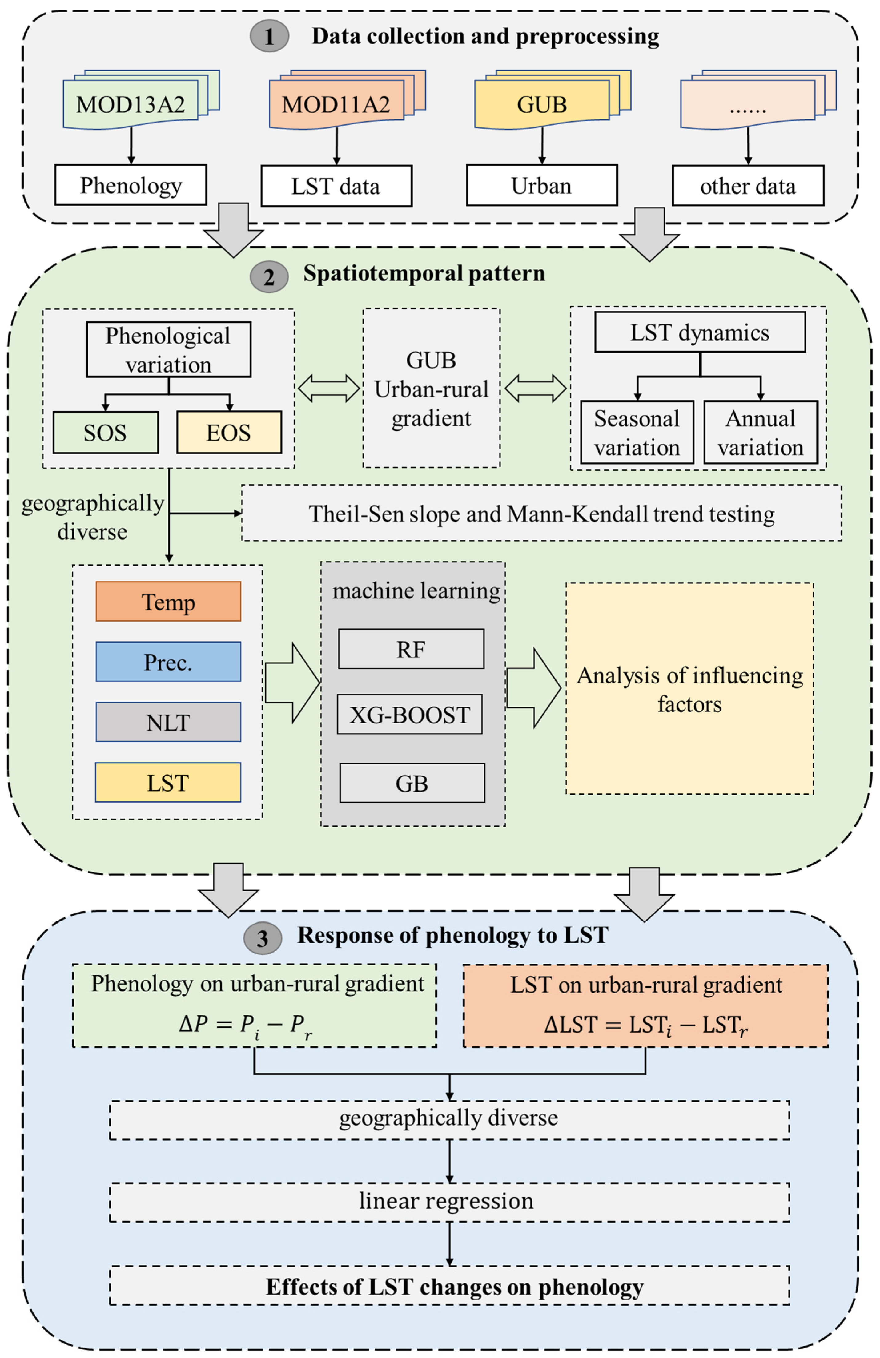
Figure 2 illustrates the methodology of this study, which involves the following steps:
(1)
Preprocessing of data was conducted using the GEE platform (https://earthengine.google.com/, accessed on 24 November 2025). The preprocessing steps included cloud masking, compositing, and smoothing to generate high-quality time series of vegetation indices suitable for phenological analysis.
(2)
Extraction and Trend Analysis of Vegetation Phenology: Based on the reconstructed time series of the EVI, phenological parameters—the SOS and EOS—were extracted using a dynamic threshold method. Subsequently, their spatial distribution patterns and long-term trends were analyzed to reveal temporal and regional variations in vegetation phenology.
(3)
Analysis of Environmental Drivers Using XGBoost–SHAP: The mechanisms through which environmental factors influence vegetation phenology in coastal and inland areas were explored using the XGBoost model combined with SHAP. This approach not only quantifies the relative importance of different environmental variables but also reveals complex nonlinear relationships and potential threshold effects between phenological parameters and their driving factors.
(4)
Urban–Rural Gradient Analysis and LST Linkage: Differences in vegetation phenology across the urban–rural gradient were examined, and their relationship with LST was further investigated to understand how urbanization affects phenological dynamics through surface thermal conditions.

2.3. Data Sources and Processing

2.3.1. Basic Data

Table 1 outlines the key data sources utilized in this study. The research utilized the Google Earth Engine [31] to download 529 satellite images of Shandong Province from 2001 to 2023. Using 1 km resolution EVI data, key phenological parameters—SOS in spring and EOS in autumn—were extracted. Additionally, daytime and nighttime average temperatures during spring and autumn were derived from the MOD11A2 dataset, and their means were calculated to represent the LST for these seasons. Urban built-up area limits were defined based on the Global Urban Boundary (GUB) dataset from the Peng Gong Research Group [32].

2.3.2. Extraction of Vegetation Phenology Metrics

Vegetation index data may not accurately represent the true seasonal growth patterns of vegetation due to factors such as sensor limitations, cloud obstruction, and atmospheric pollutants. Hence, time series processing is required to reconstruct the original EVI data. Based on TIMESAT 3.3 [33] at the pixel scale, the Savitzky–Golay (S-G) filter method [22] is applied to refine the EVI time series data. Through the iterative envelope filtering process, deviations from the normal growth trend are removed, yielding a fitted curve that better represents vegetation growth. The S-G filter equation is provided below:
Y j * = i = n n   C j Y j + 1 N
where Y j + 1 represents the j original EVI data point within the sliding window, Y j * denotes the reconstructed EVI time series data, C j is the i EVI filter coefficient, and N corresponds to the fitting order.
Based on the reconstructed EVI time series and the extraction of vegetation phenology parameters using the dynamic thresholding method. Following previous studies focused on Chinese urban areas, an amplitude threshold of 20% was predominantly adopted for phenology parameter extraction [4,9]. Additionally, to exclude outliers, this study removed pixel values with SOS greater than 180 days or less than 30 days, and EOS greater than 330 days or less than 240 days [34].

2.3.3. Analysis of Vegetation Phenology Trends

Using Theil–Sen slope (TS) and Mann–Kendall (M–K) trend tests, this study analyzes the phenological trends in Shandong Province from 2001 to 2023. TS is a non-parametric approach for calculating trends in long-term data series. The M–K is another non-parametric statistical approach commonly used to assess trend significance in time series data, offering benefits like no specific distribution requirements and reduced sensitivity to outliers [34]. The TS calculation formula is given below:
β = Median x j x i j i , j > i
where x j and x i denote the data points in the time series.
The formula for the MK is given below:
Z m = Q 1 V a r ( Q ) , Q > 0 0 , Q = 0 Q + 1 V a r ( Q ) , Q < 0
where the statistic Q is defined as:
Q = k = 1 N 1 l = k + 1 N   s i g n ( Y l Y k )
s i g n ( Y l Y k ) = 1 , Y l Y k > 0 0 , Y l Y k = 0 1 , Y l Y k < 0
V a r ( Q ) = N ( N 1 ) ( 2 N + 5 ) 18
where N represents the length of the time series, and Y represents the observed variable. The function s i g n ( Y l Y k ) used to evaluate the direction of change between paired observations. A positive value of Z m indicates an increasing trend, while a negative Z m suggests a decreasing trend.

2.3.4. Analysis of Factors Affecting Phenological Changes

XGBoost is an improved Boosting algorithm based on gradient-boosted decision trees, recognized for its fast training and high prediction performance [35]. It has gained widespread application and recognition in various research domains [36]. This algorithm optimizes the loss function using both first- and second-order gradient functions, reducing model complexity and improving training speed. In this study, the XGBoost model is employed to analyze the driving factors of phenology, with the Gradient Boosting Regressor and Random Forest Regressor used as benchmark models to assess the advantages of XGBoost in prediction performance and robustness.
Shapley Additive Explanations (SHAP) is a tool for interpreting model outputs, used to understand the impact of each feature on the model’s predictions [37]. The underlying concept is based on cooperative game theory. For each prediction sample, the SHAP model generates a “Shapley value,” which represents the total contribution of each feature.

2.3.5. Impact of Urbanization on Vegetation Phenology

Previous studies have found that the influence of urbanization on phenology typically extends within a 20 km radius [38]. To analyze the vegetation phenology changes in urban and surrounding areas, seven buffer zones were established outside the city boundaries. The urban area is defined as the region within the city boundary, while the buffer zones are categorized into suburban and rural areas [39]. This study demonstrates how phenological parameters react to urbanization by comparing the phenology of urban, suburban, and rural areas. The formula is given below:
Δ P = P i P r
where P i represents the phenological parameters within the urban and suburban buffer zones, P r represents the phenological parameters in rural, and Δ P denotes the phenological gap between urban and rural.
To examine how LST affects phenology, a method similar to the one previously described was used to calculate LST variations across urban, suburban, and rural areas. The following formula was used:
Δ L S T = L S T i L S T r
where L S T i represents the LST within the urban and suburban buffer zones, L S T r denotes the LST in rural, and Δ L S T is the gap in LST between urban and rural.
To analyze the response of vegetation phenology to surface temperature, a univariate linear regression was conducted. The expression is as follows:
y = k × x + b
where x is the LST; y is the vegetation phenology parameters; and k is the coefficient.

3. Results

3.1. Spatial Variation in Key Vegetation Phenology Indicators

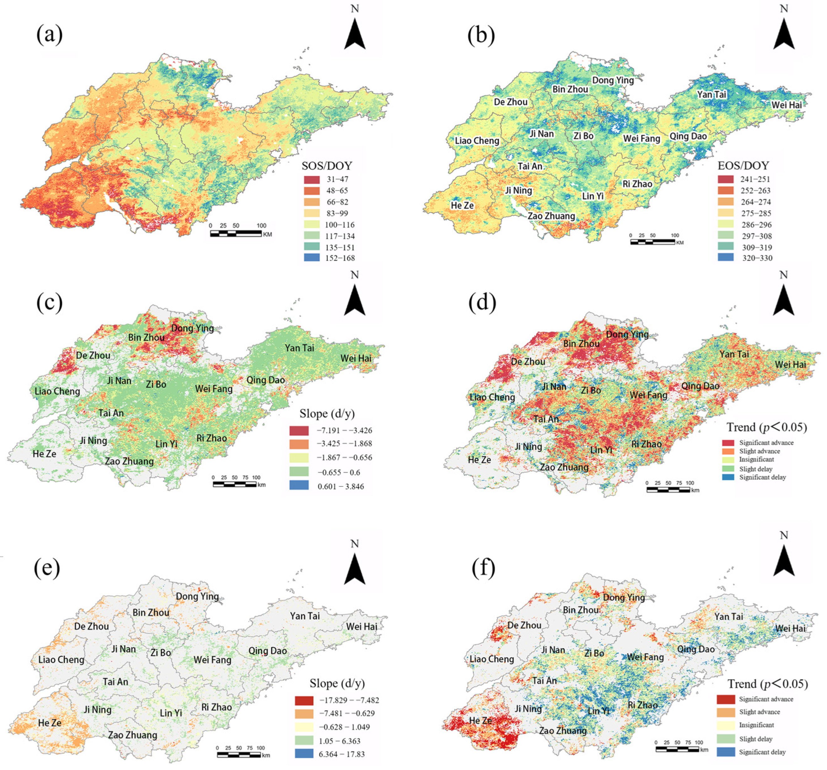
Figure 3a,b illustrate the spatial distribution of mean SOS and EOS across 16 cities in Shandong Province from 2001 to 2023 reveals pronounced inland–coastal and regional contrasts. On average, SOS occurs on day 96 and EOS on day 296. However, inland cities exhibit an earlier phenological cycle (SOS on day 86, EOS on day 292), while coastal cities experience a delayed onset and extended season (SOS on day 109, EOS on day 301). Geographically, SOS displays a west-to-east and north-to-southeast delaying trend, with the earliest onset in the west (days 31–82), moderate timing in central regions (days 83–134), and the latest in northern and southeastern cities (days 135–168). Conversely, EOS shows a southwest-to-northeast extension pattern, with the earliest end in southwestern areas (days 241–274), followed by southeastern cities (days 275–308), and the latest in central and eastern regions (days 309–330).
Temporal trends and significance levels are illustrated in Figure 3c–f. SOS shows significant advancement in northern regions, with a range of 3.42 to 7.49 days per year (d/y), while central and eastern cities display minimal delay, ranging from 0 to 0.6 d/y. In contrast, EOS trends are more heterogeneous: Heze exhibits marked advancement (0.63–7.48 d/y), whereas cities like Weifang, Qingdao, and Zibo show significant delays (1.05–6.36 d/y), indicating an extended growing season. These patterns are statistically supported, with Liaocheng, Dezhou, Binzhou, and Dongying showing significant SOS advancement (p < 0.05); Heze and Jining present significantly earlier EOS, while Weihai, Linyi, and Yantai demonstrate significantly delayed EOS (p < 0.05). Together, these results underscore the spatial heterogeneity and directional shifts in phenology, particularly the growing season lengthening in eastern and coastal cities.
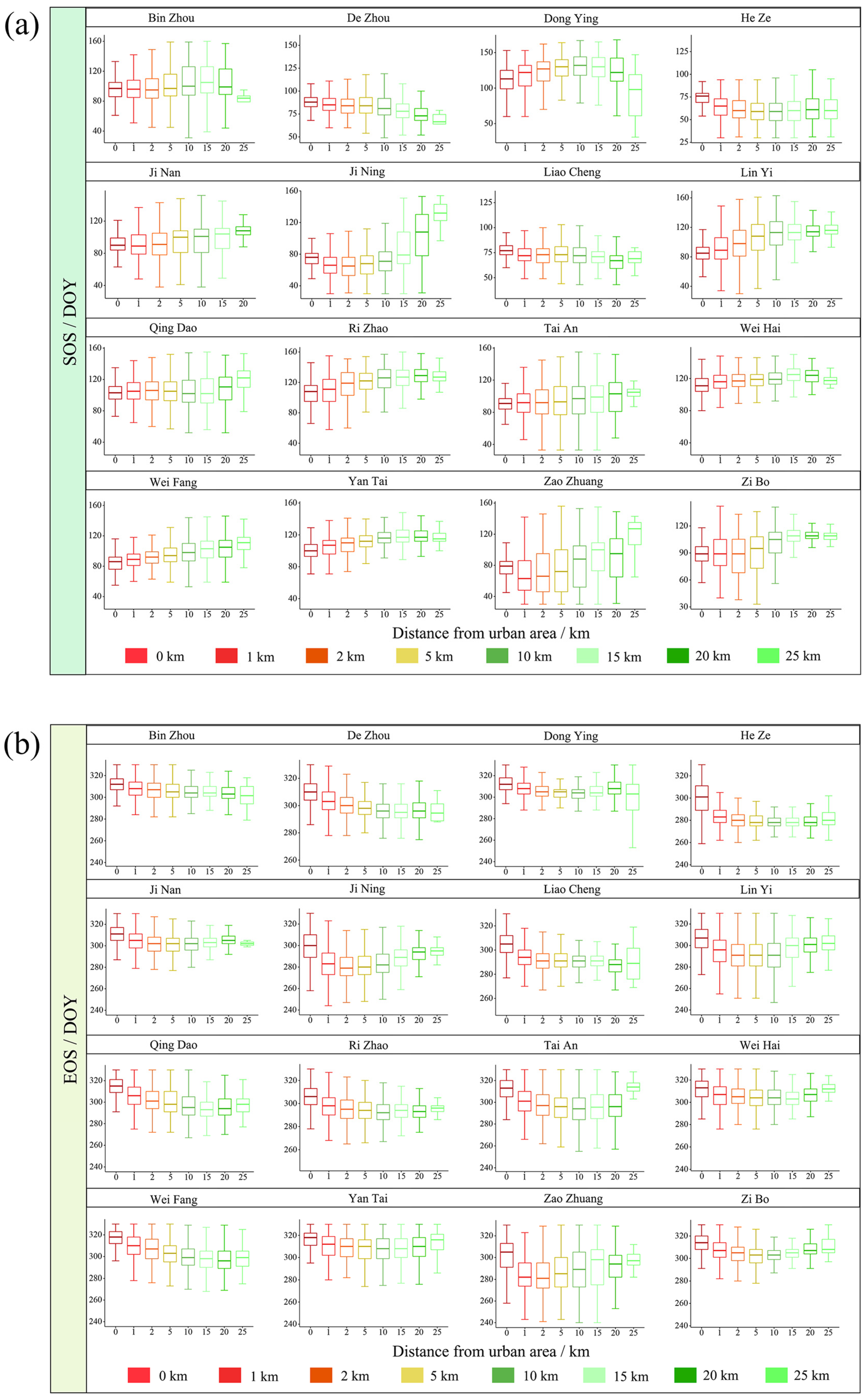
Figure 4 presents the temporal responses of phenology across urban, suburban, and rural zones in Shandong Province, reflecting the impact of urbanization intensity along a spatial gradient from city centers. On average, SOS occurs earliest in urban areas (day 91), followed by suburban (day 97) and rural regions (day 103), indicating a mean delay of 0.48 days per kilometer away from the urban core. In contrast, EOS is latest in urban areas (day 307), compared to suburban (day 295) and rural zones (day 297), advancing by approximately 0.4 days per kilometer along the same gradient. These patterns reflect a typical urbanization signal—advancing SOS and delaying EOS—consistent with an extended growing season in more urbanized environments.
Spatial heterogeneity is also evident among cities. Of the 16 cities analyzed, 11 exhibit advanced SOS closer to the urban core, while 3 show the opposite trend. For EOS, 11 cities display a delayed end of season near urban centers, whereas 5 demonstrate a mixed pattern, with initial advancement followed by delay. Notably, within 0–5 km from city centers, SOS is generally advanced, while beyond 10 km, it tends to be delayed. This spatial dynamic suggests that the influence of urbanization on phenology is strongest within the urban fringe and gradually weakens with increasing distance.
Within the 0–2 km buffer zone, urbanization exerts a pronounced effect on phenology, with significantly earlier SOS and delayed EOS, reflecting the core urban heat island effect. Beyond this zone, the phenological influence of urbanization declines and stabilizes after approximately 10 km, indicating a threshold beyond which vegetation phenology is less sensitive to urban climatic.

3.2. Phenological Sensitivity to Environmental Drivers: A Nonlinear Perspective

3.2.1. Regression Analysis and Prediction

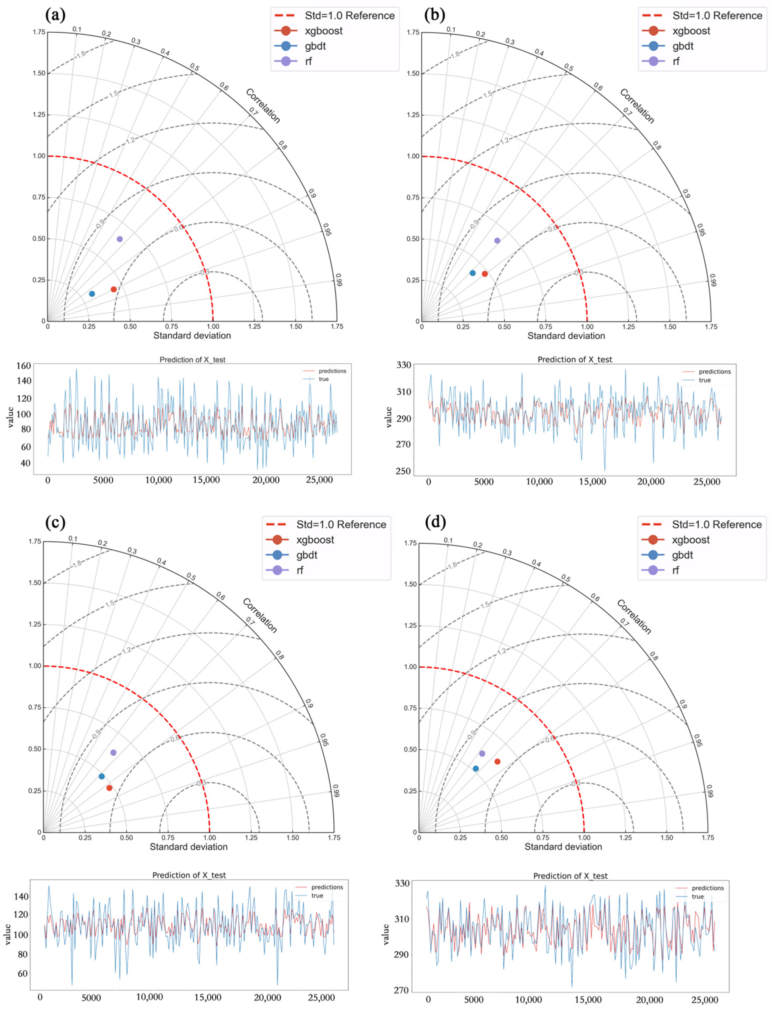
Figure 5 presents a Taylor diagram comparing the predictive performance of different machine learning models for vegetation phenology across inland and coastal regions, in both spring and autumn seasons. Among all models tested, XGBoost consistently demonstrated the highest predictive accuracy, as evidenced by superior R2 and lower RMSE values across all four datasets. Specifically, it achieved R2 values ranging from 0.73 to 0.77, and RMSE values between 8.42 and 15.68, outperforming both Gradient Boosting (GB) and Random Forest (RF) models in all scenarios. These results indicate that XGBoost not only generalizes well across diverse climatic and spatial conditions but also captures complex nonlinear relationships more effectively. Consequently, XGBoost was selected as the optimal model for predicting vegetation phenological parameters in this study.

3.2.2. Analysis of Factors Influencing Phenology

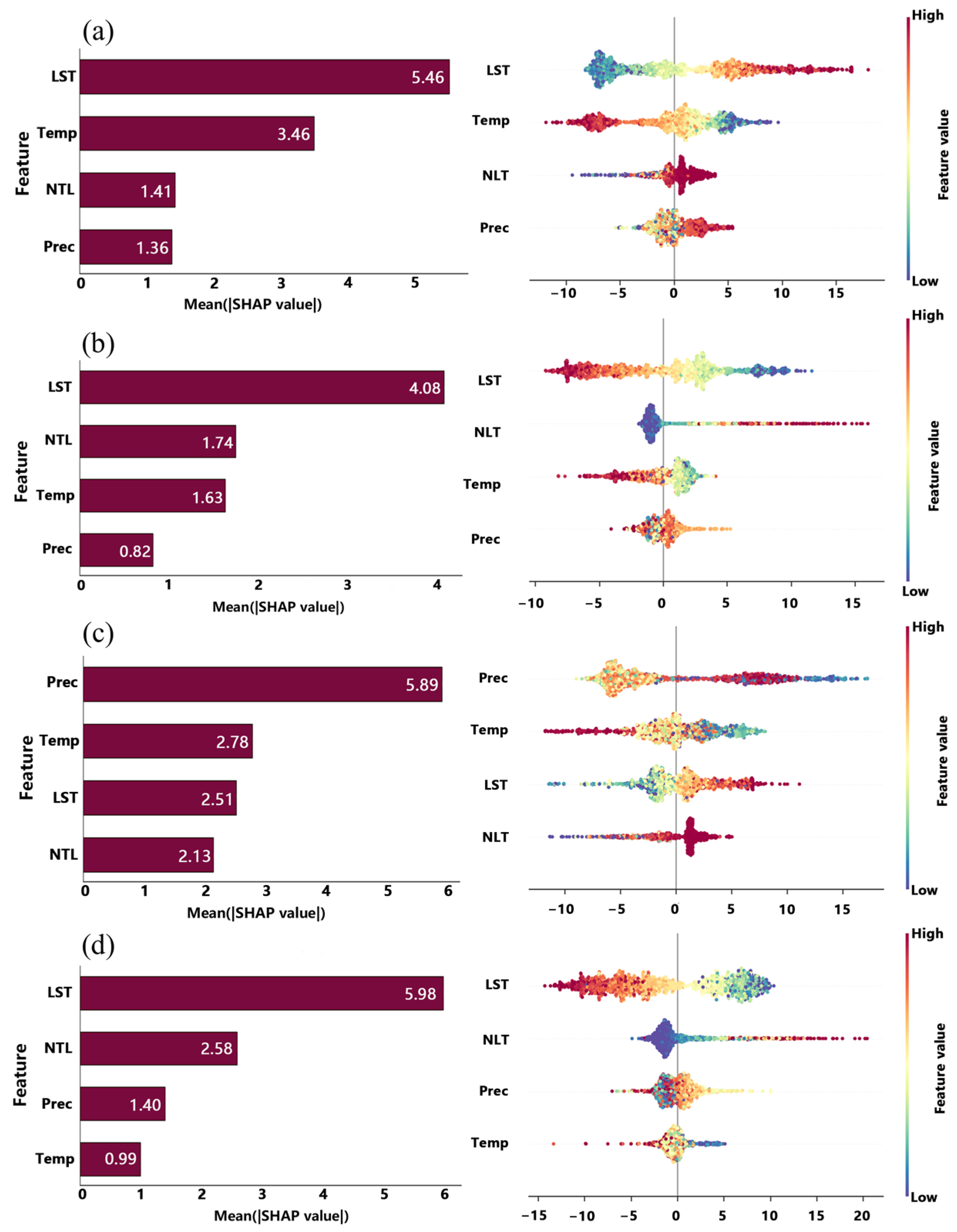
To interpret the XGBoost model and quantify the influence of different environmental drivers on vegetation phenology, the SHAP algorithm was applied (Figure 6). The left panels display the mean SHAP values, representing the relative importance of each variable, while the right-side scatter plots illustrate how feature values influence model output, with color gradients denoting variable magnitude and point position indicating direction and strength of effect.
Overall, LST emerged as the dominant predictor for inland SOS, inland EOS, and coastal EOS, whereas coastal SOS was most strongly influenced by precipitation. Temperature and nighttime lights (NTL) showed moderate and context-dependent importance across regions and phenological phases. For instance, temperature ranked second for inland SOS and coastal SOS, but played a lesser role in coastal EOS.
The SHAP scatter plots further reveal distinct nonlinear and regional-specific response patterns. High LST values strongly advanced SOS in both inland and coastal settings, particularly under elevated temperature conditions. In contrast, precipitation exhibited a strong positive contribution to coastal SOS but minimal effect in inland regions. EOS was negatively associated with both LST and temperature, suggesting their role in accelerating senescence. NTL exhibited a nonlinear impact on EOS—exerting a negative effect at low intensities and shifting to positive influence at higher levels. The relatively narrow SHAP value ranges for temperature and precipitation in EOS prediction indicate their weaker regulatory roles compared to LST and NTL.
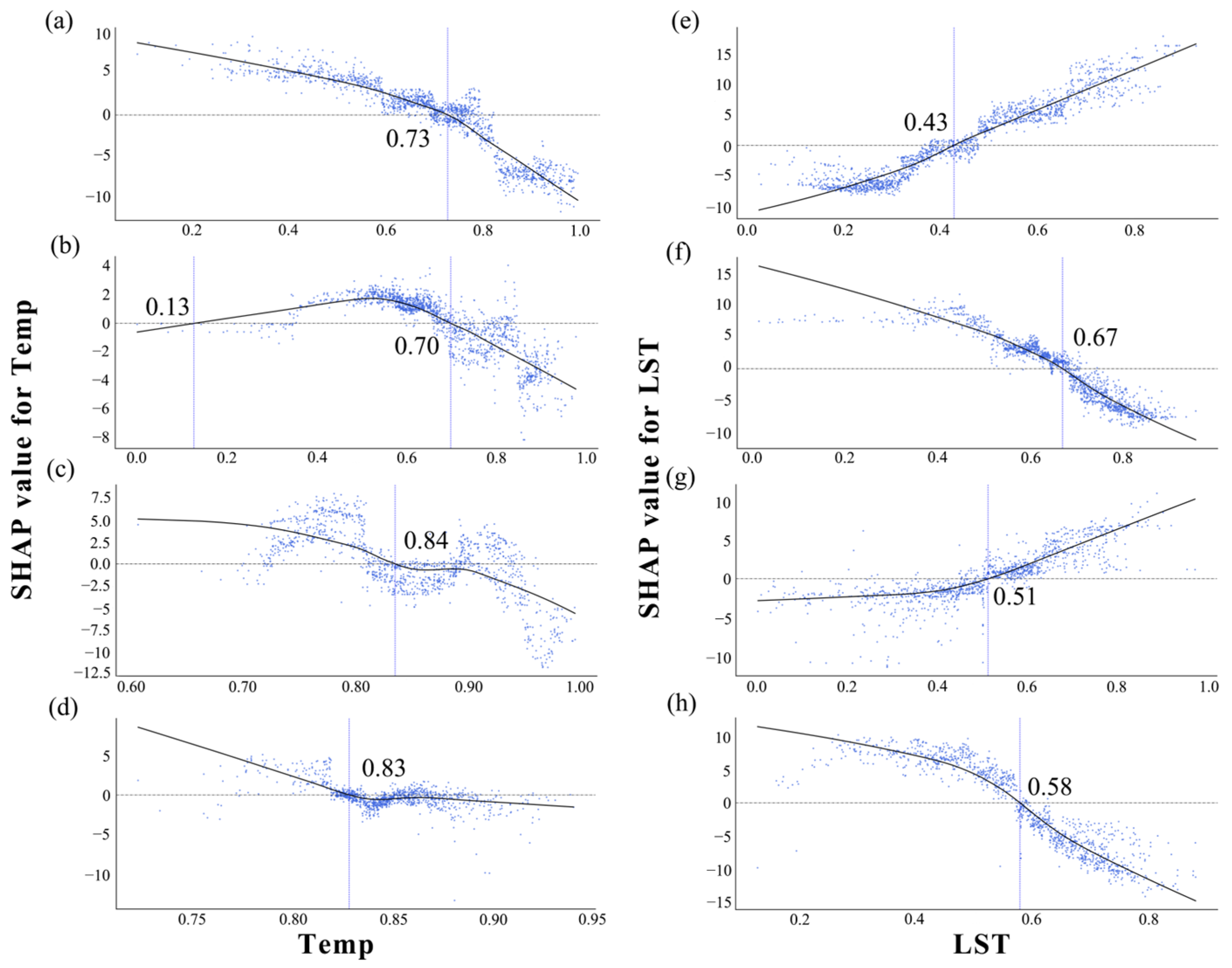
To further investigate the impact patterns of temperature and LST within different value ranges on vegetation phenology and to identify the threshold effects of these features, this study combines partial dependence plots (PDPs) and SHAP dependence plots. The changes in feature values and SHAP values are presented using LOWESS smoothing curves. The steepness of the curves reflects the marginal effect of each feature; a steeper curve indicates a stronger marginal effect of the feature. Additionally, the PDPs highlight the threshold points where the contribution of the feature to phenology shifts from negative to positive (Figure 7). The results show that the temperature threshold in the inland region is 0.7, while the threshold in the coastal region is 0.83. When temperature is below these thresholds, the contribution to vegetation phenology is positive, but it becomes negative once the threshold is exceeded. The contribution of LST to SOS shifts from negative to positive as temperature increases, with thresholds of 0.43 in inland areas and 0.51 in coastal areas. For EOS, the influence of LST on the end of the growing season changes from positive to negative as temperature increases, with identified thresholds of 0.67 in inland areas and 0.58 in coastal regions. This study reveals that while rising temperatures significantly advance SOS up to a certain threshold, exceeding this critical value may inhibit vegetation growth.

3.3. Urban–Rural Variations in Vegetation Phenology and Their Association with LST

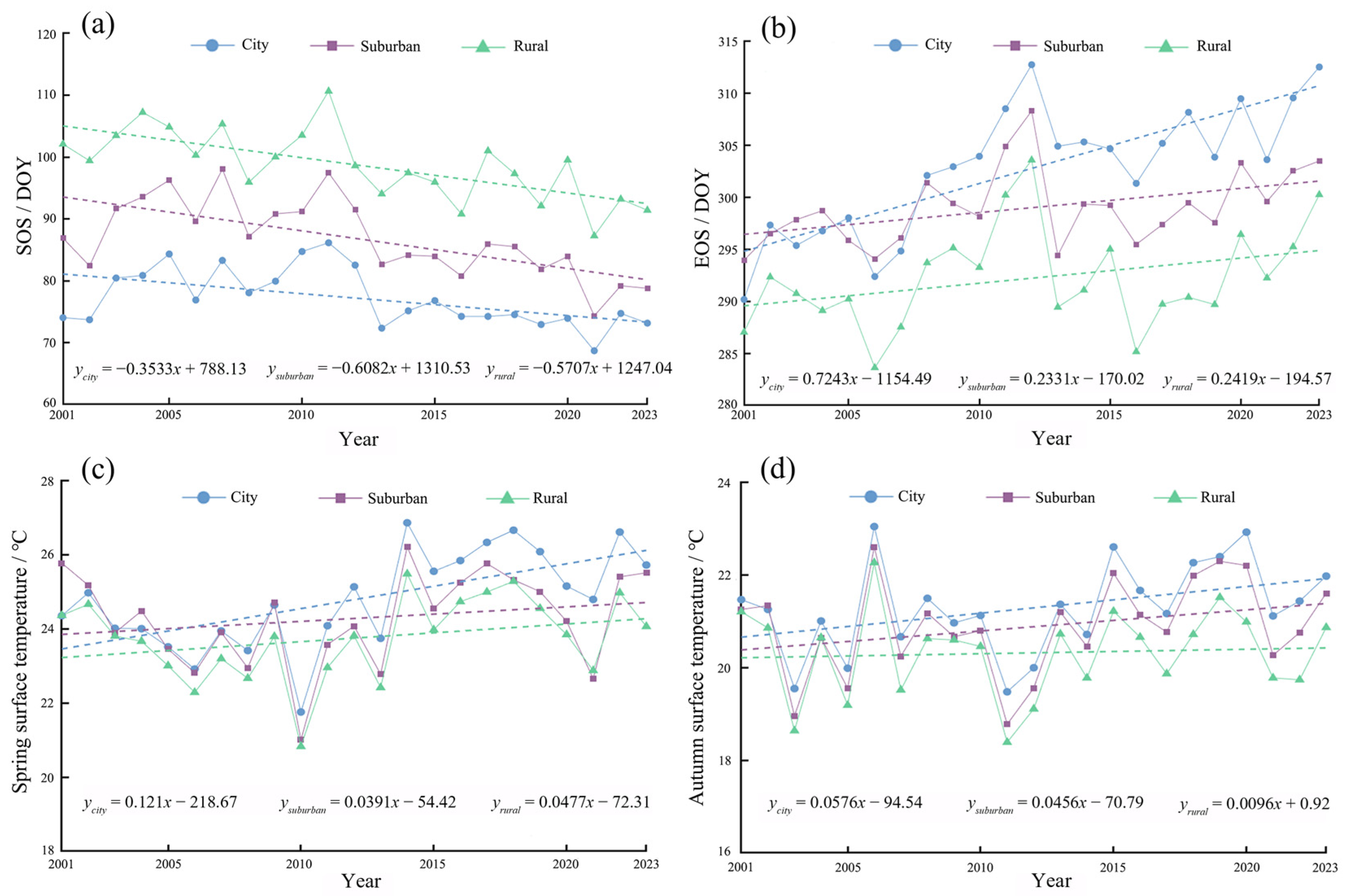
As shown in Figure 8a,b, vegetation phenology exhibited clear temporal trends across the urban–rural gradient from 2001 to 2023. Urban areas experienced a significant extension of the growing season, characterized by an advancement in SOS by 0.35 and a more pronounced delay in EOS by 0.72 d/y. Suburban and rural zones also showed advancing SOS (0.61 and 0.57 d/y, respectively), although their EOS delays were comparatively smaller (0.23 and 0.24 d/y). These patterns suggest that urbanization accelerates spring onset while more strongly postponing autumn senescence, contributing to an overall lengthening of the growing season, especially in urban environments.
Corresponding changes in LST are presented in Figure 8c,d. Urban areas exhibited the highest rates of warming, with LST increasing by 0.12 °C/year in spring and 0.06 °C/year in autumn. In contrast, suburban and rural zones experienced slower warming trends, following a consistent spatial gradient of urban > suburban > rural. Notably, the temperature rise was most pronounced in urban spring, aligning with the observed phenological shifts. These findings indicate that intensified urban warming is a key driver of asymmetric phenological changes, with stronger impacts on EOS delay than SOS advancement.
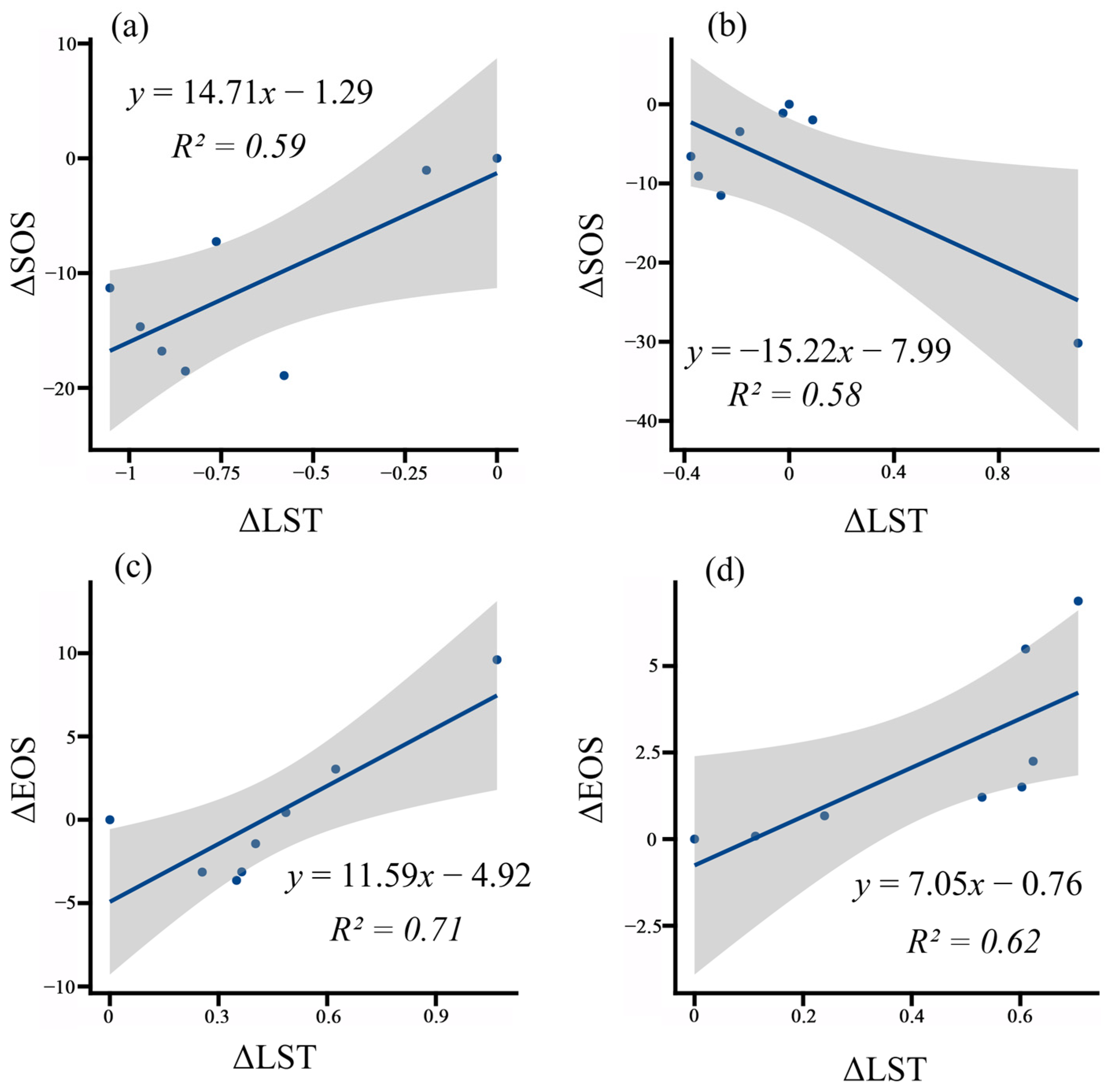
Linear regression analysis reveals significant relationships between LST and phenological parameters in both coastal and inland areas (Figure 9). For SOS, a positive correlation is observed in the coastal region, where elevated LST tends to delay the onset. In contrast, the inland region exhibits a negative relationship, with higher LST advancing SOS. For EOS, both the coastal and inland regions exhibit a positive correlation, indicating that higher LST extends the EOS. Overall, the results demonstrate that the coastal region responds more strongly to LST than the inland region, highlighting the regulatory role of regional climate backgrounds in phenological changes.

4. Discussion

4.1. Spatiotemporal Variability in Vegetation Phenology Across Urban and Rural Landscapes

Between 2001 and 2023, significant spatial heterogeneity in SOS and EOS was observed across 16 cities in Shandong Province, driven by urban–rural gradients in both coastal and inland areas. The results indicate that SOS and EOS occur earlier in inland regions compared to coastal ones, likely due to the continental climate and more pronounced temperature fluctuations inland. Spring temperatures rise quickly, leading to an earlier onset of SOS, while autumn temperatures drop rapidly, causing EOS to occur earlier [40]. Along the urban–rural gradient, cities with higher development levels exhibit significantly earlier SOS and delayed EOS near urban cores. However, in some inland cities like Dezhou and Heze, SOS advances in areas farther from the city center. Precipitation is widely regarded as one of the most important factors influencing vegetation growth and carbon balance at the regional scale. Some research has found that excessive moisture delays SOS in the North China Plain [41]. Frequent human activities in urban areas can lead to the urban heat island effect and changes in land cover types, which, in turn, influence the timing of urban vegetation phenology. Furthermore, suburban areas, as the radiating influence range of urbanization, also experience changes in vegetation phenology, although the impact is less pronounced compared to urban areas. This study reveals that in cities like Jinan and Zibo, the EOS in the 0–5 km buffer zone from the city center tends to advance, while beyond this zone, EOS is delayed. This is because, within a certain distance along the urban–rural gradient, urbanization has the most significant impact on vegetation growth, and as the distance increases, the influence diminishes [42]. Previous research has shown that urbanization exerts its strongest influence on vegetation phenology within a 0–2 km radius of the city center [38]. The results of this study further corroborate that the most substantial urbanization-induced changes in vegetation phenology are concentrated within this central buffer zone. Furthermore, a comparison of the results from this study with those from the Yangtze River Delta and the Guangdong–Hong Kong–Macau Greater Bay Area reveals similar vegetation phenology responses to urbanization in Shandong, such as earlier SOS and later EOS with increasing urbanization. However, Shandong exhibits more pronounced spatial differences in phenological responses due to the coastal–inland climate gradient, whereas the other two regions show more homogeneous urban heat island effects [43,44].

4.2. Synergistic Effects of Climate Change and Urbanization Factors

Nighttime light intensity, acting as a proxy for urbanization level [45], showed a complex bidirectional regulatory effect on vegetation phenology. At low intensities, nighttime lights may suppress normal plant growth through light pollution [8], leading to an advancement of EOS. At higher intensities, the persistent heat emissions from nighttime lighting exacerbate urban thermal conditions, thereby postponing the timing of vegetation phenological events. This phenomenon is particularly evident in coastal regions, highlighting the combined influence of artificial light pollution and elevated urban temperatures on the timing of vegetation phenological responses during the urbanization process.
LST and air temperature are key drivers of shifts in vegetation phenology; however, their effects are not consistently in the same direction [15]. Earlier research indicates that excessive temperatures beyond a critical threshold may suppress vegetative development, thereby postponing the onset of the growing season. The feature threshold analysis in this study revealed the key mechanisms through which LST and temperature impact phenology. The threshold analysis illustrates how changes in temperature and LST shift from negative to positive impacts under specific conditions, significantly influencing vegetation phenology. Suitable surface temperatures benefit plants by allowing them to accumulate sufficient photosynthetic products and energy reserves, thereby altering phenology [46]. The differences in thresholds between inland and coastal regions reflect their distinct ecological and climatic characteristics. Inland areas, due to their geographic distance from the ocean, experience drier climates and more extreme temperature fluctuations, making vegetation phenology more sensitive to temperature changes. As a result, even lower temperatures and LST can significantly advance or delay vegetation phenology. In contrast, coastal areas, influenced by a more temperate marine climate [47], have higher thresholds for temperature changes, indicating stronger buffering capacity and adaptability.
Precipitation’s role was also revealed to be highly region-specific. A key finding from our SHAP analysis (Figure 6c) was that precipitation, not temperature, emerged as the dominant driver for coastal SOS, contrasting sharply with the temperature-driven inland regions. This points to a critical ecological mechanism tied to the maritime climate: unlike the continental inland regions where spring temperature accumulation is the primary limiting factor, coastal areas experience a buffered spring warming due to the ocean’s high thermal capacity. In this thermally moderated environment, temperature accumulation becomes a less variable and thus less critical trigger. Conversely, the North China Plain, including coastal Shandong, is known for high inter-annual precipitation variability [48]. Therefore, the timing and adequacy of water availability likely acts as the primary limiting factor for initiating the growing season in this specific coastal environment.

4.3. Variations in How LST Influences Vegetation Phenology Across the Urban-to-Suburban Continuum

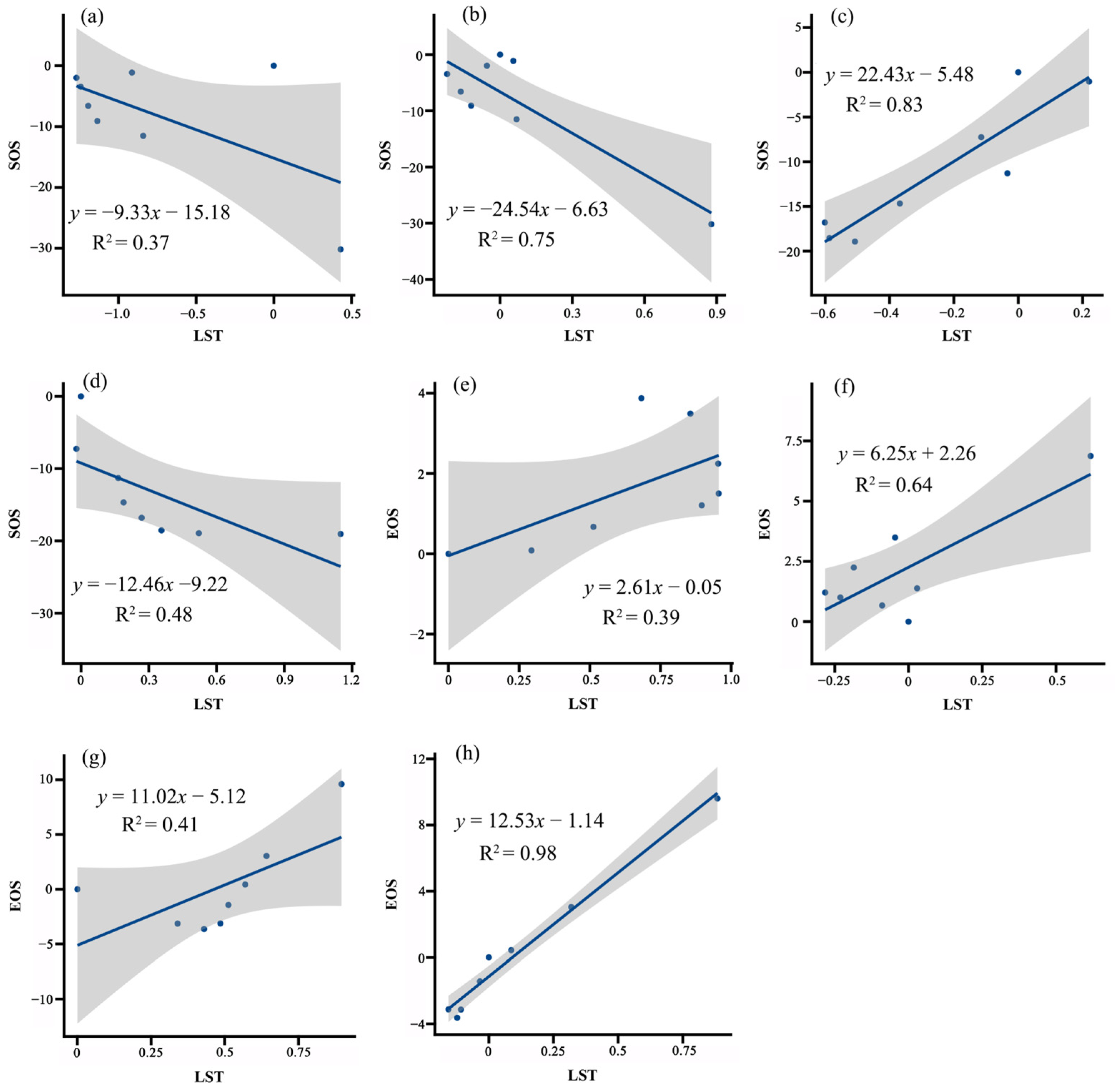
It has been shown that daytime and nighttime thermal conditions exert contrasting influences on leaf senescence [49,50]. This study focuses on coastal and inland cities, where daytime and nighttime LST may play more significant roles in different regions. Based on this, the study further analyzes daytime and nighttime LST in coastal and inland cities to explore their influence on vegetation phenology, with the results shown in Figure 10. The impact of LST variation on the SOS shows significant differences between regions. Specifically, in inland areas, higher nighttime LST tends to promote plant growth by enhancing nocturnal respiration and metabolic processes [51]. In contrast, in coastal areas, higher daytime LST inhibits vegetation growth due to increased evaporation and heat stress, which may negatively affect photosynthesis and plant productivity [52]. Additionally, higher nighttime LST in coastal areas may promote plant growth by reducing nighttime cold stress. Rising LST are consistently associated with a delayed EOS, with nighttime LST exerting a stronger influence than daytime values in both study areas. This delay is likely due to the fact that warmer nighttime temperatures can extend the growing season by preventing early frost events and enhancing plant metabolic activity [53].
Urban regions generally undergo stronger warming driven by the urban heat island phenomenon, which contributes to a later EOS or earlier SOS of the growing season [54]. In inland regions, higher spring LST in urban areas tends to advance the SOS, whereas elevated autumn LST is associated with a delayed EOS [21]. In contrast, in coastal areas, LST and SOS show a positive correlation, where higher LST actually delays SOS. This may be due to the moderating influence of the marine climate in coastal regions, where temperature increases lead to changes in evaporation and precipitation patterns [55], thereby delaying the onset of the growing season.

4.4. Validation and Scale-Dependency of Urban Phenological Gradients

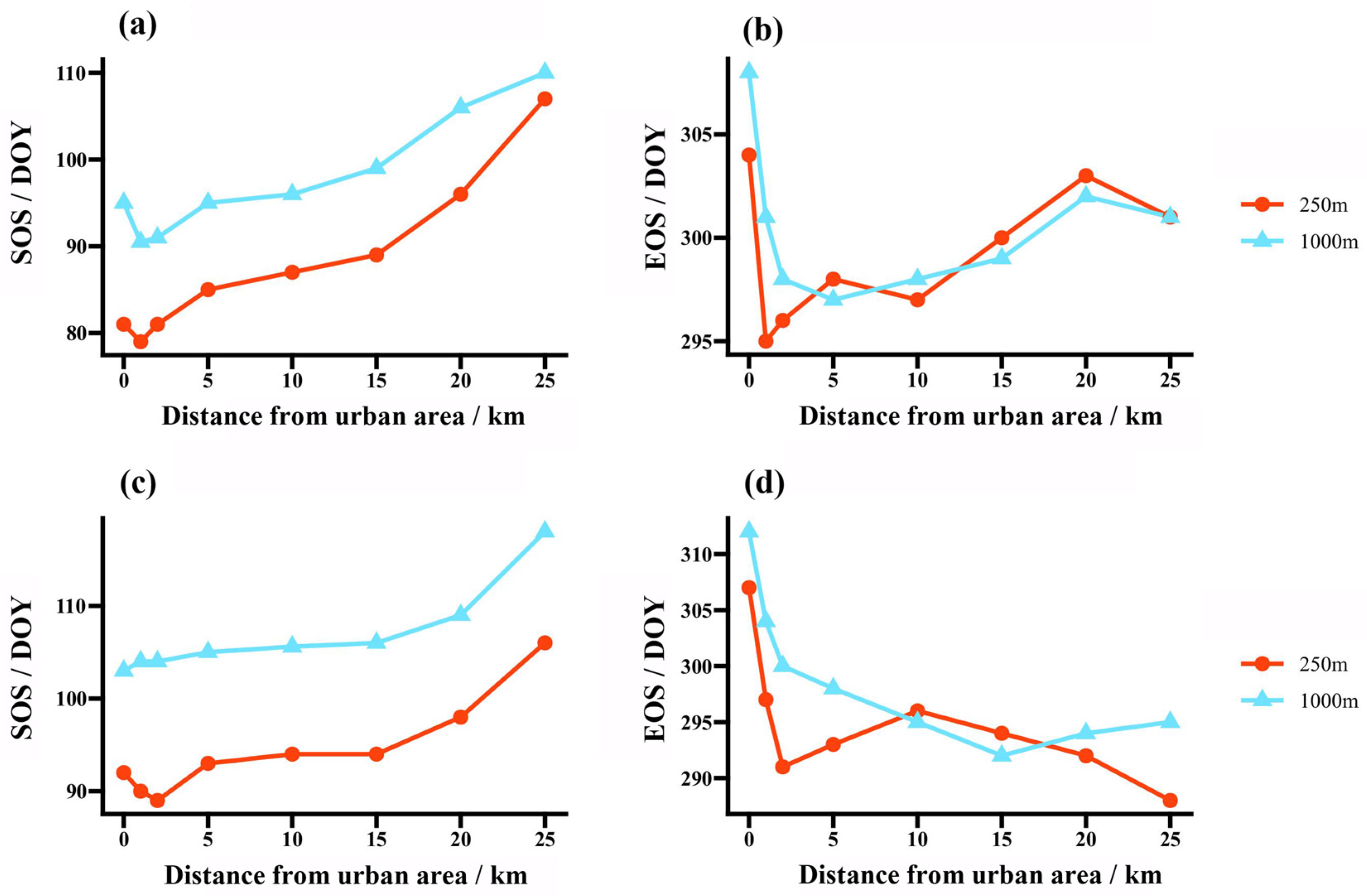
To investigate the potential influence of spatial resolution on our findings, we conducted a validation experiment using 250 m MODIS EVI data [56] for Jinan and Qingdao (Figure 11). This comparison confirms our core conclusion is robust: both datasets show that urbanization delays EOS and advances SOS. However, the 250 m data reveals a much stronger signal, indicating the 1000 m mixed-pixel effect significantly underestimates the true magnitude of the Urban Heat Island’s impact [57]. For instance, in Qingdao (Figure 11d), the 250 m data shows a sharp ~17-day EOS difference between the core and inner suburb, whereas the 1000 m data captured only a ~5-day difference. This also confirms a systematic bias in absolute dates between the two scales, a finding that is consistent with the results of most studies on phenological scale effects [58,59]. Most importantly, the 250 m data unmasks complex spatial heterogeneity that the 1000 m data averages out. While the 1000 m data presents a simplified, near–linear decline, the 250 m data reveals a more complex, nonlinear trend for Qingdao’s EOS (Figure 11d). This complex pattern likely reflects the true, fine-scale urban structure. This validation confirms that our primary 1000 m analysis provides a robust but conservative estimate of urbanization’s impact, while the true effects are stronger and more spatially complex.

4.5. Policy Recommendations

Drawing on the outcomes of this research, we put forward the following policy recommendations aimed at tackling the challenges posed by urbanization and climate change:
(1)
To alleviate the heat warming effect—especially in densely built-up and coastal zones—it is advisable to expand the presence of vegetation and open water systems within urban environments [60]. Expanding the coverage of vegetation and aquatic features can effectively lower local temperatures, improve the urban microclimate, and enhance the resilience of urban ecosystems.
(2)
Implement Differentiated Temperature Control Strategies. Based on our findings of distinct temperature response thresholds in coastal versus inland regions (Figure 7), policies must be region-specific. Inland areas should focus on soil and water conservation and greening efforts to reduce the role of temperature fluctuations on phenology. In coastal areas, natural resources such as sea breezes should be utilized to enhance the unique climatic regulating effect, mitigating the negative impacts of temperature increases due to urbanization on the ecosystem.
(3)
Establish Green Buffer Zones: Creating green buffer zones in suburban areas can improve connectivity between urban and rural ecosystems, promoting ecological mobility and biodiversity.

4.6. Limitations and Uncertainties

MOD13A2 EVI satellite-derived data were employed to monitor variations in vegetation phenological patterns. While remote sensing imagery is an effective tool for large-scale vegetation phenology studies, its relatively low spatial resolution may not accurately capture phenological changes in urban areas with sparse or highly mixed vegetation cover, and there may be discrepancies with field observations at the species level [30]. Second, and more importantly, our analysis did not incorporate a land cover classification to distinguish between different vegetation types, our results therefore represent the composite phenological signal from this mixed landscape. Additionally, we did not exclude farmland, although most cities in Shandong Province are surrounded by agricultural land [61]. Farmland phenology is significantly influenced by crop types and human activities, which may introduce uncertainty in phenological values for nonurban areas [62].
Future research should adopt a more integrated methodological framework to overcome the limitations of the current analysis. First, to address the lack of robust validation, finer-scale satellite imagery should be employed in conjunction with systematic in situ phenological observations from sources such as meteorological station networks. This integration is essential for the rigorous validation of the extracted SOS and EOS metrics and for calibrating phenological thresholds across diverse vegetation types. Second, to strengthen the attribution of the observed trends, two major confounding factors must be addressed. The impact of farmland phenology, which is heavily driven by anthropogenic management, must be more explicitly isolated and quantified. Concurrently, the influence of short-term extreme climate events, including droughts, must be statistically disentangled from the long-term signals attributed to urbanization.

5. Conclusions

This study investigates how vegetation phenology varies across the urban–rural continuum in both coastal and inland regions. By analyzing 16 cities in Shandong Province, this study reveals the nonlinear influences of climatic variables and urban development on vegetation phenological patterns, addressing a gap in the literature that has largely ignored urbanization impacts and regional geographic differences. This study not only contributes to the theoretical understanding of vegetation phenology but also offers valuable insights and guidance for urban ecological management.
The results show that: (1) From 2001 to 2023, the average SOS in Shandong Province occurred on day 91, and the average EOS occurred on day 296. SOS and EOS occurred earlier in inland regions than in coastal zones. Vegetation SOS in the western and southwestern regions started earliest, while EOS in the eastern and northeastern regions ended latest. (2) In 11 cities, vegetation SOS occurred earlier closer to the urban core, whereas in 14 cities, EOS tended to be later in more urbanized zones. Across all sites, the average change in SOS was an advancement of 0.48 days per kilometer from rural to urban areas, while EOS showed a delay of 0.4 days per kilometer along the same gradient. (3) Temperature is a key factor in influencing vegetation phenology. Rather than inducing linear changes, rising temperatures demonstrate a notable threshold effect on phenological responses. (4) Vegetation phenology in coastal areas shows greater sensitivity to LST, with daytime and nighttime LST influencing plant responses differently when compared to inland regions.

Author Contributions

Data Processing, X.M.; Formal Analysis, X.M. and Z.L.; Methodology, Z.L. and X.M.; Validation, J.K. and Z.Z.; Visualization, Z.L. and L.Z.; Funding Acquisition, Y.C.; Original Draft Preparation, X.M.; Review and Editing, Z.W., Z.Z. and J.W. All authors have read and agreed to the published version of the manuscript.

Funding

This work is supported by the National Earth Observation Science Data Center 2024 Open Research Project (NODAOP2024002), the Ministry of Education Humanities and Social Sciences Planning Fund Project (21YJAZH009), the National Natural Science Foundation of China (42401432) and the Guangzhou Basic and Applied Basic Research (2024A04J3666).

Data Availability Statement

The original contributions presented in this study are included in the article. Further inquiries can be directed to the corresponding author.

Conflicts of Interest

The authors declare no conflicts of interest.

References

  1. Angel, S.; Parent, J.; Civco, D.L.; Blei, A.; Potere, D. The dimensions of global urban expansion: Estimates and projections for all countries, 2000–2050. Prog. Plan. 2011, 75, 53–107. [Google Scholar] [CrossRef]
  2. van Vliet, J. Direct and indirect loss of natural area from urban expansion. Nat. Sustain. 2019, 2, 755–763. [Google Scholar] [CrossRef]
  3. Ullah, M.; Li, J.; Wadood, B. Analysis of Urban Expansion and its Impacts on Land Surface Temperature and Vegetation Using RS and GIS, A Case Study in Xi’an City, China. Earth Syst. Environ. 2020, 4, 583–597. [Google Scholar] [CrossRef]
  4. Ren, Q.; He, C.; Huang, Q.; Zhou, Y. Urbanization Impacts on Vegetation Phenology in China. Remote Sens. 2018, 10, 1905. [Google Scholar] [CrossRef]
  5. Zhong, Q.; Ma, J.; Zhao, B.; Wang, X.; Zong, J.; Xiao, X. Assessing spatial-temporal dynamics of urban expansion, vegetation greenness and photosynthesis in megacity Shanghai, China during 2000–2016. Remote Sens. Environ. 2019, 233, 111374. [Google Scholar] [CrossRef]
  6. Liu, Q.; Fu, Y.H.; Zeng, Z.; Huang, M.; Li, X.; Piao, S. Temperature, precipitation, and insolation effects on autumn vegetation phenology in temperate China. Glob. Chang. Biol. 2016, 22, 644–655. [Google Scholar] [CrossRef]
  7. Caparros-Santiago, J.A.; Rodriguez-Galiano, V.; Dash, J. Land surface phenology as indicator of global terrestrial ecosystem dynamics: A systematic review. ISPRS J. Photogramm. Remote Sens. 2021, 171, 330–347. [Google Scholar] [CrossRef]
  8. Meng, L.; Mao, J.; Zhou, Y.; Richardson, A.D.; Lee, X.; Thornton, P.E.; Ricciuto, D.M.; Li, X.; Dai, Y.; Shi, X.; et al. Urban warming advances spring phenology but reduces the response of phenology to temperature in the conterminous United States. Proc. Natl. Acad. Sci. USA 2020, 117, 4228–4233. [Google Scholar] [CrossRef]
  9. Li, S.; Li, Q.; Zhang, J.; Zhang, S.; Wang, X.; Yang, S.; Zhang, S. Study on the Spatial and Temporal Distribution of Urban Vegetation Phenology by Local Climate Zone and Urban–Rural Gradient Approach. Remote Sens. 2023, 15, 3957. [Google Scholar] [CrossRef]
  10. Li, P.; Peng, C.; Wang, M.; Luo, Y.; Li, M.; Zhang, K.; Zhang, D.; Zhu, Q. Dynamics of vegetation autumn phenology and its response to multiple environmental factors from 1982 to 2012 on Qinghai-Tibetan Plateau in China. Sci. Total Environ. 2018, 637–638, 855–864. [Google Scholar] [CrossRef]
  11. Zheng, C.; Tang, X.; Gu, Q.; Wang, T.; Wei, J.; Song, L.; Ma, M. Climatic anomaly and its impact on vegetation phenology, carbon sequestration and water-use efficiency at a humid temperate forest. J. Hydrol. 2018, 565, 150–159. [Google Scholar] [CrossRef]
  12. Piao, S.; Fang, J.; Zhou, L.; Ciais, P.; Zhu, B. Variations in satellite—Derived phenology in China’s temperate vegetation. Glob. Chang. Biol. 2006, 12, 672–685. [Google Scholar] [CrossRef]
  13. Shen, M.; Wang, S.; Jiang, N.; Sun, J.; Cao, R.; Ling, X.; Fang, B.; Zhang, L.; Zhang, L.; Xu, X.; et al. Plant phenology changes and drivers on the Qinghai–Tibetan Plateau. Nat. Rev. Earth Environ. 2022, 3, 633–651. [Google Scholar] [CrossRef]
  14. Qiao, C.; Shen, S.; Cheng, C.; Wu, J.; Jia, D.; Song, C. Vegetation Phenology in the Qilian Mountains and Its Response to Temperature from 1982 to 2014. Remote Sens. 2021, 13, 286. [Google Scholar] [CrossRef]
  15. Ma, R.; Shen, X.; Zhang, J.; Xia, C.; Liu, Y.; Wu, L.; Wang, Y.; Jiang, M.; Lu, X. Variation of vegetation autumn phenology and its climatic drivers in temperate grasslands of China. Int. J. Appl. Earth Obs. Geoinf. 2022, 114, 103064. [Google Scholar] [CrossRef]
  16. Workie, T.G.; Debella, H.J. Climate change and its effects on vegetation phenology across ecoregions of Ethiopia. Glob. Ecol. Conserv. 2018, 13, e00366. [Google Scholar] [CrossRef]
  17. Han, G.; Xu, J. Land surface phenology and land surface temperature changes along an urban-rural gradient in Yangtze River Delta, China. Environ. Manag. 2013, 52, 234–249. [Google Scholar] [CrossRef] [PubMed]
  18. Sun, J.; Wang, X.; Chen, A.; Ma, Y.; Cui, M.; Piao, S. NDVI indicated characteristics of vegetation cover change in China’s metropolises over the last three decades. Environ. Monit. Assess. 2011, 179, 1–14. [Google Scholar] [CrossRef]
  19. Wang, L.; De Boeck, H.J.; Chen, L.; Song, C.; Chen, Z.; McNulty, S.; Zhang, Z. Urban warming increases the temperature sensitivity of spring vegetation phenology at 292 cities across China. Sci. Total Environ. 2022, 834, 155154. [Google Scholar] [CrossRef]
  20. Zhang, C.C.; Meng, D.; Li, X.J. Spatial and temporal changes of vegetation phenology and its response to urbanization in the Beijing-Tianjin-Hebei region. Acta Ecol. Sin. 2023, 43, 249–262. [Google Scholar] [CrossRef]
  21. Liu, Z.; Zhou, Y.; Feng, Z. Response of vegetation phenology to urbanization in urban agglomeration areas: A dynamic urban-rural gradient perspective. Sci. Total Environ. 2023, 864, 161109. [Google Scholar] [CrossRef]
  22. Yang, Y.; Qiu, X.; Yang, L.; Lee, D. Impacts of Thermal Differences in Surfacing Urban Heat Islands on Vegetation Phenology. Remote Sens. 2023, 15, 5133. [Google Scholar] [CrossRef]
  23. Ma, J.; Wang, J.; He, S.; Zhang, J.; Liu, L.; Zhong, X. Direct and indirect effects of urbanization on vegetation: A survey of Yunnan central urban Economic Circle, China. Ecol. Indic. 2024, 166, 112536. [Google Scholar] [CrossRef]
  24. Yang, J.; Xin, J.; Zhang, Y.; Xiao, X.; Xia, J.C. Contributions of sea–land breeze and local climate zones to daytime and nighttime heat island intensity. NPJ Urban. Sustain. 2022, 2, 12. [Google Scholar] [CrossRef]
  25. Jiang, Q.; Yuan, Z.; Yin, J.; Yao, M.; Qin, T.; Lü, X.; Wu, G.; Ning, Z. Response of vegetation phenology to climate factors in the source region of the Yangtze and Yellow Rivers. J. Plant Ecol. 2024, 17, rtae046. [Google Scholar] [CrossRef]
  26. Li, C.; Wang, R.; Cui, X.; Wu, F.; Yan, Y.; Peng, Q.; Qian, Z.; Xu, Y. Responses of vegetation spring phenology to climatic factors in Xinjiang, China. Ecol. Indic. 2021, 124, 107286. [Google Scholar] [CrossRef]
  27. Shi, Y.; Jin, N.; Ma, X.; Wu, B.; He, Q.; Yue, C.; Yu, Q. Attribution of climate and human activities to vegetation change in China using machine learning techniques. Agric. For. Meteorol. 2020, 294, 108146. [Google Scholar] [CrossRef]
  28. Vidal-Macua, J.J.; Nicolau, J.M.; Vicente, E.; Moreno-de Las Heras, M. Assessing vegetation recovery in reclaimed opencast mines of the Teruel coalfield (Spain) using Landsat time series and boosted regression trees. Sci. Total Environ. 2020, 717, 137250. [Google Scholar] [CrossRef] [PubMed]
  29. Zaimes, G.N.; Gounaridis, D.; Symenonakis, E. Assessing the impact of dams on riparian and deltaic vegetation using remotely-sensed vegetation indices and Random Forests modelling. Ecol. Indic. 2019, 103, 630–641. [Google Scholar] [CrossRef]
  30. Chen, Y.; Lin, M.; Lin, T.; Zhang, J.; Jones, L.; Yao, X.; Geng, H.; Liu, Y.; Zhang, G.; Cao, X.; et al. Spatial heterogeneity of vegetation phenology caused by urbanization in China based on remote sensing. Ecol. Indic. 2023, 153, 110448. [Google Scholar] [CrossRef]
  31. Tamiminia, H.; Salehi, B.; Mahdianpari, M.; Quackenbush, L.; Adeli, S.; Brisco, B. Google Earth Engine for geo-big data applications: A meta-analysis and systematic review. ISPRS J. Photogramm. Remote Sens. 2020, 164, 152–170. [Google Scholar] [CrossRef]
  32. Li, X.; Gong, P.; Zhou, Y.; Wang, J.; Bai, Y.; Chen, B.; Hu, T.; Xiao, Y.; Xu, B.; Yang, J.; et al. Mapping global urban boundaries from the global artificial impervious area (GAIA) data. Environ. Res. Lett. 2020, 15, 094044. [Google Scholar] [CrossRef]
  33. Zhang, J.; Shang, R.; Rittenhouse, C.; Witharana, C.; Zhu, Z. Evaluating the impacts of models, data density and irregularity on reconstructing and forecasting dense Landsat time series. Sci. Remote Sens. 2021, 4, 100023. [Google Scholar] [CrossRef]
  34. Peng, Z.; Jiang, D.; Li, W.; Mu, Q.; Li, X.; Cao, W.; Shi, Z.; Chen, T.; Huang, J. Impacts of the scale effect on quantifying the response of spring vegetation phenology to urban intensity. Remote Sens. Environ. 2024, 315, 114485. [Google Scholar] [CrossRef]
  35. Chen, T.; Guestrin, C. Xgboost: A scalable tree boosting system. In Proceedings of the 22nd ACM Sigkdd International Conference on Knowledge Discovery and Data Mining, San Francisco, CA, USA, 13–17 August 2016; pp. 785–794. [Google Scholar]
  36. Huang, F.; Zhang, J.; Zhou, C.; Wang, Y.; Huang, J.; Zhu, L. A deep learning algorithm using a fully connected sparse autoencoder neural network for landslide susceptibility prediction. Landslides 2019, 17, 217–229. [Google Scholar] [CrossRef]
  37. Zhang, J.; Ma, X.; Zhang, J.; Sun, D.; Zhou, X.; Mi, C.; Wen, H. Insights into geospatial heterogeneity of landslide susceptibility based on the SHAP-XGBoost model. J. Environ. Manag. 2023, 332, 117357. [Google Scholar] [CrossRef]
  38. Jia, W.; Zhao, S.; Zhang, X.; Liu, S.; Henebry, G.M.; Liu, L. Urbanization imprint on land surface phenology: The urban-rural gradient analysis for Chinese cities. Glob. Chang. Biol. 2021, 27, 2895–2904. [Google Scholar] [CrossRef]
  39. Zhou, D.; Zhao, S.; Zhang, L.; Liu, S. Remotely sensed assessment of urbanization effects on vegetation phenology in China’s 32 major cities. Remote Sens. Environ. 2016, 176, 272–281. [Google Scholar] [CrossRef]
  40. Gao, X.; Zhao, D. Impacts of climate change on vegetation phenology over the Great Lakes Region of Central Asia from 1982 to 2014. Sci. Total Environ. 2022, 845, 157227. [Google Scholar] [CrossRef]
  41. Ji, S.; Ren, S.; Li, Y.; Dong, J.; Wang, L.; Quan, Q.; Liu, J. Diverse responses of spring phenology to preseason drought and warming under different biomes in the North China Plain. Sci. Total Environ. 2021, 766, 144437. [Google Scholar] [CrossRef]
  42. Ji, Y.; Zhan, W.; Du, H.; Wang, S.; Li, L.; Xiao, J.; Liu, Z.; Huang, F.; Jin, J. Urban-rural gradient in vegetation phenology changes of over 1500 cities across China jointly regulated by urbanization and climate change. ISPRS J. Photogramm. Remote Sens. 2023, 205, 367–384. [Google Scholar] [CrossRef]
  43. Yang, Y.; Fan, F. Land surface phenology and its response to climate change in the Guangdong-Hong Kong-Macao Greater Bay Area during 2001–2020. Ecol. Indic. 2023, 154, 110728. [Google Scholar] [CrossRef]
  44. Zhu, E.; Fang, D.; Chen, L.; Qu, Y.; Liu, T. The Impact of Urbanization on Spatial–Temporal Variation in Vegetation Phenology: A Case Study of the Yangtze River Delta, China. Remote Sens. 2024, 16, 914. [Google Scholar] [CrossRef]
  45. Levin, N.; Kyba, C.C.M.; Zhang, Q.; Sánchez de Miguel, A.; Román, M.O.; Li, X.; Portnov, B.A.; Molthan, A.L.; Jechow, A.; Miller, S.D.; et al. Remote sensing of night lights: A review and an outlook for the future. Remote Sens. Environ. 2020, 237, 111443. [Google Scholar] [CrossRef]
  46. Moore, C.E.; Meacham-Hensold, K.; Lemonnier, P.; Slattery, R.A.; Benjamin, C.; Bernacchi, C.J.; Lawson, T.; Cavanagh, A.P. The effect of increasing temperature on crop photosynthesis: From enzymes to ecosystems. J. Exp. Bot. 2021, 72, 2822–2844. [Google Scholar] [CrossRef]
  47. Hasan, M.K.; Kumar, L. Yield trends and variabilities explained by climatic change in coastal and non-coastal areas of Bangladesh. Sci. Total Environ. 2021, 795, 148814. [Google Scholar] [CrossRef]
  48. Li, H.; Liu, S.; Yin, M.; Zhu, L.a.; Shen, E.; Sun, B.; Wang, S. Spatial and temporal variability and risk assessment of regional climate change in northern China: A case study in Shandong Province. Nat. Hazards 2022, 111, 2749–2786. [Google Scholar] [CrossRef]
  49. Meng, L.; Zhou, Y.; Li, X.; Asrar, G.R.; Mao, J.; Wanamaker, A.D.; Wang, Y. Divergent responses of spring phenology to daytime and nighttime warming. Agric. For. Meteorol. 2020, 281, 107832. [Google Scholar] [CrossRef]
  50. Wu, C.; Wang, X.; Wang, H.; Ciais, P.; Peñuelas, J.; Myneni, R.B.; Desai, A.R.; Gough, C.M.; Gonsamo, A.; Black, A.T.; et al. Contrasting responses of autumn-leaf senescence to daytime and night-time warming. Nat. Clim. Chang. 2018, 8, 1092–1096. [Google Scholar] [CrossRef]
  51. Jing, P.; Wang, D.; Zhu, C.; Chen, J. Plant Physiological, Morphological and Yield-Related Responses to Night Temperature Changes across Different Species and Plant Functional Types. Front. Plant Sci. 2016, 7, 1774. [Google Scholar] [CrossRef]
  52. Bal, S.K.; Minhas, P.S. Atmospheric stressors: Challenges and coping strategies. In Abiotic Stress Management for Resilient Agriculture; Springer: Singapore, 2017; pp. 9–50. [Google Scholar] [CrossRef]
  53. Abbas, A.; Rossi, S.; Huang, B. Plant metabolic responses and adaptation mechanisms to elevated night temperature associated with global warming. Grass Res. 2024, 4, e015. [Google Scholar] [CrossRef]
  54. Ding, H.; Xu, L.; Elmore, A.J.; Shi, Y. Vegetation Phenology Influenced by Rapid Urbanization of The Yangtze Delta Region. Remote Sens. 2020, 12, 1783. [Google Scholar] [CrossRef]
  55. Dai, A.; Zhao, T.; Chen, J. Climate Change and Drought: A Precipitation and Evaporation Perspective. Curr. Clim. Chang. Rep. 2018, 4, 301–312. [Google Scholar] [CrossRef]
  56. Zhang, H.; Wang, X.; Peng, D. Evaluation of Urban Vegetation Phenology Using 250 m MODIS Vegetation Indices. Photogramm. Eng. Remote Sens. 2022, 88, 461–467. [Google Scholar] [CrossRef]
  57. Zhao, L.; Fan, X.; Hong, T. Urban Heat Island Effect: Remote Sensing Monitoring and Assessment—Methods, Applications, and Future Directions. Atmosphere 2025, 16, 791. [Google Scholar] [CrossRef]
  58. Ma, M.; Liu, J.; Liu, M.; Zhu, W.; Atzberger, C.; Lv, X.; Dong, Z. Quantitative Assessment of the Spatial Scale Effects of the Vegetation Phenology in the Qinling Mountains. Remote Sens. 2022, 14, 5749. [Google Scholar] [CrossRef]
  59. Liu, L.; Cao, R.; Shen, M.; Chen, J.; Wang, J.; Zhang, X. How Does Scale Effect Influence Spring Vegetation Phenology Estimated from Satellite-Derived Vegetation Indexes? Remote Sens. 2019, 11, 2137. [Google Scholar] [CrossRef]
  60. Xu, X.; Liu, S.; Sun, S.; Zhang, W.; Liu, Y.; Lao, Z.; Guo, G.; Smith, K.; Cui, Y.; Liu, W.; et al. Evaluation of energy saving potential of an urban green space and its water bodies. Energy Build. 2019, 188–189, 58–70. [Google Scholar] [CrossRef]
  61. Yin, P.; Li, X.; Mao, J.; Johnson, B.A.; Wang, B.; Huang, J. A comprehensive analysis of the crop effect on the urban-rural differences in land surface phenology. Sci. Total Environ. 2023, 861, 160604. [Google Scholar] [CrossRef]
  62. Li, L.; Li, X.; Asrar, G.; Zhou, Y.; Chen, M.; Zeng, Y.; Li, X.; Li, F.; Luo, M.; Sapkota, A.; et al. Detection and attribution of long-term and fine-scale changes in spring phenology over urban areas: A case study in New York State. Int. J. Appl. Earth Obs. Geoinf. 2022, 110, 102815. [Google Scholar] [CrossRef]
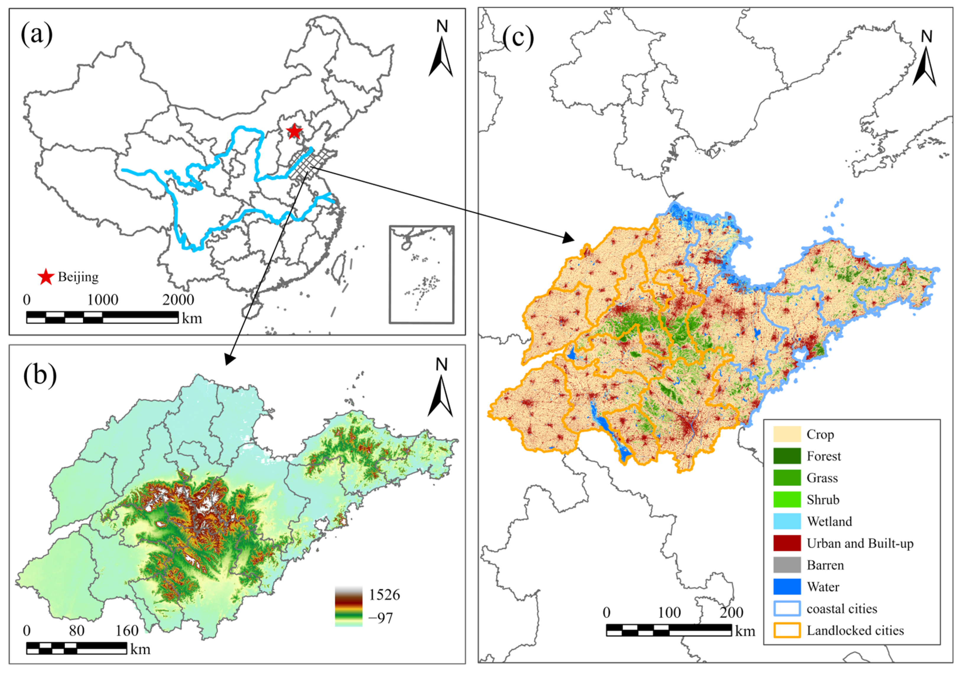
Figure 1. Study Area: (a) Spatial Location of Shandong Province, (b) DEM, (c) Land Use.
Remotesensing 17 03833 g001
Figure 2. Workflow of This Study.
Remotesensing 17 03833 g002
Figure 3. Annual SOS and EOS Spatial Distribution for Urban Vegetation: (a) SOS, (b) EOS, (c) SOS Trends, (d) SOS Significance, (e) EOS Trends, (f) EOS Significance.
Remotesensing 17 03833 g003
Figure 4. Spatiotemporal Variations in Vegetation SOS and EOS Across 16 Cities Along the Urban–Rural Gradient: (a) SOS, (b) EOS.
Remotesensing 17 03833 g004
Figure 5. Comparison of Model Accuracy: (a) Inland SOS, (b) Inland EOS, (c) Coastal SOS, (d) Coastal EOS.
Remotesensing 17 03833 g005
Figure 6. Feature importance and contribution distribution: (a) Inland SOS, (b) Inland EOS, (c) Coastal SOS, (d) Coastal EOS.
Remotesensing 17 03833 g006
Figure 7. Nonlinear Relationships between Temperature and Phenology: (ad) Inland Spring Temperature, Inland Autumn Temperature, Coastal Spring Temperature, Coastal Autumn Temperature; (eh) Inland Spring LST, Inland Autumn LST, Coastal Spring LST, Coastal Autumn LST.
Remotesensing 17 03833 g007
Figure 8. Inter-annual Trends in Vegetation Phenology and LST: (a) SOS, (b) EOS, (c) Spring LST, (d) Autumn LST.
Remotesensing 17 03833 g008
Figure 9. Regression between LST and phenological metrics across coastal and inland regions: (a) SOS—Coastal, (b) SOS—Inland, (c) EOS—Coastal, (d) EOS—Inland.
Remotesensing 17 03833 g009
Figure 10. The Relationship between LST and Phenology: (a) Spring daytime LST in inland areas, (b) Spring nighttime LST in inland areas, (c) Spring daytime LST in Coastal areas, (d) Spring nighttime LST in Coastal areas, (e) Autumn daytime LST in inland areas, (f) Autumn nighttime LST in inland areas, (g) Autumn daytime LST in Coastal areas, (h) Spring nighttime LST in Coastal areas.
Remotesensing 17 03833 g010
Figure 11. Comparison of urban–rural gradients for 1000 m and 250 m data: (a,b) Jinan, (c,d) Qingdao.
Remotesensing 17 03833 g011
Table 1. Description of Various Datasets.
Data NameData SourceResolutionTime Range
EVI (MOD13A2)https://www.earthdata.nasa.gov/data/catalog/lpcloud-mod13a2-061, accessed on 25 November 202516 d, 1 km2001–2023
LST (MOD11A2)https://www.earthdata.nasa.gov/data/catalog/lpcloud-mod11a2-061, accessed on 25 November 20258 d, 1 km2001–2023
GUBhttp://data.starcloud.pcl.ac.cn/, accessed on 25 November 202530 m2018
Land Usehttps://zenodo.org/records/8239305, accessed on 25 November 202530 m2001–2023
China 1 km monthly mean temperature datasethttps://data.tpdc.ac.cn/, accessed on 25 November 2025Monthly, 1 km2001–2023
China 1 km monthly precipitation datasethttps://data.tpdc.ac.cn/, accessed on 25 November 2025Monthly, 1 km2001–2023
DEMhttp://www.gscloud.cn/, accessed on 25 November 202530 m-
nighttime lighthttps://dataverse.harvard.edu/, accessed on 25 November 20251 km2001–2023
Disclaimer/Publisher’s Note: The statements, opinions and data contained in all publications are solely those of the individual author(s) and contributor(s) and not of MDPI and/or the editor(s). MDPI and/or the editor(s) disclaim responsibility for any injury to people or property resulting from any ideas, methods, instructions or products referred to in the content.