Framework for Processing of CRISM Hyperspectral Data for Global Martian Mineralogy

Highlights

What are the main findings?

• Processing CRISM hyperspectral data remains challenging due to high dimensionality and striping noise; this study presents a framework for global mineralogical mapping by implementing filtering and algorithmic optimization to improve the generation of spectral cluster maps (SCMs).
• The adaptation and automation of previously manual procedures, such as determining the optimal number of clusters, enable the efficient and reproducible production of global mineralogical maps.

What are the implications of the main findings?

• The robust clustering process now allows the large-scale generation of mineralogical maps in the form of SCMs from CRISM data.
• The proposed framework builds the basis for an automated processing pipeline, enabling a scalable, global mineralogical analysis of the Martian surface without the need for manual intervention.

Abstract

Hyperspectral data from CRISM have proven invaluable for analyzing the mineralogical composition of the Martian surface. However, processing such datasets remains challenging due to their high dimensionality and systematic noise, such as striping artifacts caused by the pushbroom imaging technique. Building on previous research, this study introduces a framework that forms the basis for an automated pipeline that combines preprocessing, dimensionality reduction using UMAP, k-means clustering, and an adaptive stripe correction filter to generate mineral maps of the Martian surface. Additionally, the pipeline integrates a noise variance estimation step based on PCA to assess the feasibility and expected efficacy of stripe removal before applying the filter. We validate the methodology across multiple CRISM datasets, including regions such as Jezero Crater, Nili Fossae, and Mawrth Vallis. Comparative analyses using metrics such as the CH index, DB index, and SC demonstrate improved clustering performance and robust mineralogical mapping, which indicates a step toward more reliable and automated clustering of CRISM data. Furthermore, the pipeline leverages spectral libraries for automated mineral classification, yielding results comparable to expert-defined maps while addressing discrepancies caused by residual noise or clustering limitations. This study represents a step toward fully automated, scalable geospatial analysis of CRISM Martian surface data, offering a robust framework for processing large hyperspectral datasets and supporting future planetary exploration missions. In the future, we intend to deploy an automated analysis pipeline as a freely accessible web service.

1. Introduction

The Compact Reconnaissance Imaging Spectrometer for Mars (CRISM) onboard NASA’s Mars Reconnaissance Orbiter (MRO) has provided a wealth of hyperspectral data for analyzing the mineralogical composition of the Martian surface [1]. These data have been instrumental in detecting aqueous alteration minerals and identifying past environmental conditions [2]. Automated analysis of CRISM data would be particularly valuable in the context of planetary habitability assessments, as it could enable systematic, large-scale identification of mineral assemblages indicative of past aqueous environments [3]. In particular, the Jezero Crater region has been extensively studied due to its geological diversity and the presence of a well-preserved delta, making it a prime target for the Perseverance rover mission [4,5,6]. However, data analysis is still a manual task, as efficient and scalable methods for processing and clustering CRISM hyperspectral data remain a challenge due to the high dimensionality of the datasets and the presence of systematic noise, including striping artifacts [7,8]. These artifacts arise due to slight variations in the sensitivity of individual detector elements within the pushbroom imaging sensor, causing visible vertical stripes in the image data. Such systematic errors complicate the analysis by introducing non-physical patterns that can obscure the actual spectral signatures of surface minerals.

Unsupervised machine learning techniques have proven effective in extracting meaningful spectral clusters from hyperspectral data, aiding in the interpretation of Martian mineralogy [9,10]. Previous studies have demonstrated that combining Uniform Manifold Approximation and Projection (UMAP) with k-means clustering provides effective dimensionality reduction and outperforms alternative approaches such as t-SNE or hybrid clustering methods, yielding robust spectral cluster maps (SCMs) [9,11]. These maps provide an efficient way to segment and classify surface materials based on spectral signatures, reducing the need for manual interpretation.

SCMs segment hyperspectral data into distinct spectral classes, representing different surface materials or minerals based on their spectral similarity [11]. Typically a combination of dimensionality reduction and clustering algorithms are used to generate SCMs. However, a crucial limitation of these approaches lies in their relatively low degree of automation. Key processing steps, such as the determination of the optimal number of clusters and the tuning of algorithmic parameters, are often performed manually. Yet this directly influences the quality and interpretability of the resulting mineral maps. Too few clusters may oversimplify the mineralogical diversity, obscuring important geological features, whereas too many clusters might lead to redundancy and ambiguous interpretations. This dependence on expert judgment not only reduces scalability but also limits reproducibility across different datasets. As a result, the potential for large-scale, fully automated mineralogical mapping of the Martian surface remains underexploited. To overcome these limitations, an automated and systematic approach for reliable, reproducible mineralogical mapping is essential. However, achieving this level of automation remains challenging due to the complexity of Martian hyperspectral data and the diversity of mineral signatures. One of the key limitations of previous methodologies is their sensitivity to systematic noise, particularly striping artifacts introduced by the pushbroom imaging technique used in CRISM observations [12]. These artifacts can significantly degrade clustering performance and lead to misclassification of spectral features.

Building on these previous investigations [9,11], this study addresses three critical research questions: Firstly, how can the mineralogical mapping process be further automated to efficiently handle extensive CRISM datasets without relying on manual intervention? This includes developing a robust pipeline that minimizes human input while maintaining geological interpretability and ensuring regional adaptability across diverse Martian terrains. Secondly, how can existing approaches be further improved through optimized hyperparameter selection? Thirdly, how can systematic noise, particularly the persistent striping artifacts inherent to pushbroom imaging, be effectively eliminated or significantly mitigated? To address this issue, we incorporate an adaptive striping correction filter based on wavelet and Fourier analysis [13,14]. Additionally, we employ Principal Component Analysis (PCA) to estimate the underlying noise variance before filtering, allowing us to assess whether stripe removal is likely to be effective in a given dataset.

By integrating optimized dimensionality reduction, automated cluster selection, and a noise-aware striping filter, our approach enhances the robustness and scalability of spectral clustering of Martian surface data. The proposed methodology was evaluated using multiple CRISM datasets, confirming its robustness and general applicability beyond Jezero Crater to a range of mineralogically diverse Martian terrains. The results provide an improved basis for large-scale geospatial analysis of Martian surface composition, potentially aiding future landing site selection and in situ exploration, particularly as subsurface access becomes a key criterion in site evaluation [15].

The remainder of this paper is structured as follows: Section 2 describes the data sources and preprocessing steps, including the striping correction filter and the clustering methods. Section 3 presents the clustering results and a comparative analysis of performance metrics, while also introducing a refined mineral classification approach based on reference spectral libraries. In Section 4 we discuss our findings and noise variance estimation, introducing it as a metric to better evaluate the effectiveness of the striping filter across different datasets. Additionally we discuss the implications of this methodology for future Mars exploration and geologic mapping efforts.

2. Materials and Methods

This section focuses on the optimized UMAP algorithm, filtering process to mitigate stripe artifacts, and the approach used to determine the optimal number of clusters. Additionally, it provides a description of the data set and its source.

2.1. Data Source and Location

CRISM is a high-resolution visible and infrared mapping spectrometer currently in orbit around Mars aboard NASA’s Mars Reconnaissance Orbiter (MRO) [1]. For this analysis, we used CRISM hyperspectral MTRDR data products, as further detailed in

Table A5. List of investigated CRISM observations and their corresponding regions, noise variance and filter performance.

CRISM ID	Region	Noise Variance	Filter Class
hrl00013347	Elysium Catena	0.291885	3
frt00008a4a	Sisyphi Cavi	0.155814	2
frt0000a0b2	Aureum Chaos	0.205942	2
frt000093ed	Ius Chasma	0.153497	1
frt0001784d	Galaxias	0.526070	3
hrl00013a04	Melas Dorsa	0.646710	3
frt00007847	Tantalus Fluctus	0.131418	2
frt00009047	Pyrrhae Fossae	0.154375	2
frt0001bc88	Baetis Labes	0.267655	2
frt00007e28	Noctis Labyrinthus	0.085311	2
hrl0000cf8e	Olympus	0.291727	3
hrl0001900c	Xanthe Montes	0.275637	2
frt00009de7	Peneus Palus	0.217910	3
frt0001de11	Nili Patera	0.542054	3
frt000049f5	Hellas Planitia	0.133856	2
frt0000cb17	Nilokeras Scopulus	0.287090	2
frt000089de	Axius Valles	0.396712	3
frt0001678a	Valles Marineris	0.223134	2
frt00003e12	Nili Fossae	0.027719	1
frt00009a16	Oxia Planum	0.165179	1
frt0000810d	Oxia Planum	0.210821	2
frt0000654f	Ritchey Crater	0.260078	2
hrl0000baba	Gale	0.368135	2
hrl000040ff	Jezero Crater	0.077085	1
frt0000aa7d	Mawrth Vallis	0.150482	1

. These are pre-processed data sets that have been empirically and statistically corrected to remove spikes, rectify imaging geometry and gimbal motion, and eliminate atmospheric contamination, resulting in an approximation of surface reflectance [1]. In addition, the MTRDR processing pipeline includes corrections for instrument-specific effects such as the spectral smile (wavelength-dependent geometric distortion across the detector) and applies the volcano-scan atmospheric correction method [16]. MTRDR products represent therefore the most standardized and physically interpretable CRISM datasets, already approximating surface reflectance and ensuring comparability across regions. Accordingly, MTRDR products provide a stable and consistent input for automated analysis while avoiding sensor and atmospheric effects that would otherwise distort PCA-based noise estimation and UMAP embeddings. Thus, the additional processing steps introduced here complement, rather than duplicate, the existing corrections. The data sets depict specific targets and in 2D spatially resolved spectra form 362 $\mathrm{n}$$\mathrm{m}$ to 3920 $\mathrm{n}$$\mathrm{m}$. Spatial resolution ranges from 18 $\mathrm{m}$/px to 36 $\mathrm{m}$/px, varying with observation mode.

In addition, Pelkey et al. [17] and Viviano et al. [18] describe a feature set of “image products” derived from CRISM spectra, which are closely related to the mineralogical composition of the Martian surface. Our objective is to develop a methodology capable of generating mineral maps for the entire Martian surface.

To evaluate the generalization capability of the proposed method, three geologically and mineralogically distinct regions were selected. However, to ensure comparability with previous studies, the focus is on the region of Jezero Crater. Jezero Crater, a 45 km-wide basin near Nili Fossae (e.g., [4,19,20,21]), is characterized not only by carbonate- and phyllosilicate-bearing sediments but also by its well-preserved fluvial delta, which records multiple phases of sediment transport and lacustrine activity [4,5]. This deltaic system is one of the primary reasons for its selection as the landing site of NASA’s Perseverance rover mission. It is challenging to obtain expert-validated ground truth maps for local Martian mineralogy, as in-situ sampling is not feasible. Therefore, this study focuses on regions for which previous mineralogical assessments have been conducted, using these as comparative references.

In addition to Jezero Crater, a region directly within Nili Fossae will be examined. In contrast, the Nili Fossae region represents one of the largest olivine- and carbonate-bearing outcrops on Mars [21], showing a wide mineralogical diversity including phyllosilicates, hydrated opal, and amorphous silicates [22]. As a third region of our study, we include an area within Mawrth Vallis. Mawrth Vallis differs markedly from both sites and is dominated by thick, stratified phyllosilicate sequences and Fe/Mg-smectites overlain by Al-rich clays such as kaolinite [23]. Moreover, the Mawrth Vallis region is of particular astrobiological interest and represents the proposed landing site of the ExoMars Rosalind Franklin rover, which will deploy a 2 m subsurface drill to investigate past environmental conditions and search for biosignatures. This site has been extensively studied in the context of ExoMars driven research on indicators and methods for reconstructing ancient Martian environments [24,25].

These variations in mineralogy and morphology ensure that the selected areas differ significantly in both mineralogical composition and topography. The detailed locations of the investigated regions can be seen in Figure 1. A summary of the selected CRISM observations is provided in the Table A5.

Figure 1. Overview of regions analyzed in this work. (A): Mars Global Digital Image Color Mosaic of the Nili Fossae region, including Jezero Crater. (B): IR-enhanced color composite (FAL) for CRISM dataset HRL000040FF of Jezero Crater. (C): CRISM FAL image of dataset FRT00003E12 in Nili Fossae. (D): Region of Mawrth Vallis visualized from Mars Global Digital Image Color Mosaic. (E): CRISM FAL image of dataset FRT0000AA7D.

Figure 1. Overview of regions analyzed in this work. (A): Mars Global Digital Image Color Mosaic of the Nili Fossae region, including Jezero Crater. (B): IR-enhanced color composite (FAL) for CRISM dataset HRL000040FF of Jezero Crater. (C): CRISM FAL image of dataset FRT00003E12 in Nili Fossae. (D): Region of Mawrth Vallis visualized from Mars Global Digital Image Color Mosaic. (E): CRISM FAL image of dataset FRT0000AA7D.

2.2. Analysis Pipeline

The clustering methods employed here build upon the foundations established in our previous work [9]. Accordingly, the fundamental processing pipeline, consisting of data preprocessing, dimensionality reduction, and clustering, remains consistent with prior approaches. To address the three research questions outlined above, this study introduces three key methodological advancements: Firstly, an optimized implementation of the UMAP algorithm, specifically tuned for improved performance on CRISM datasets. Secondly, an adaptive stripe correction filter (see Section 2.3) aimed at mitigating systematic vertical noise patterns. And thirdly, an automated post-processing method to determine the optimal number of clusters based on quantitative metrics (see Section 2.4).

Regarding preprocessing, we closely follow the established methodology introduced by Gao et al. [10], involving pixel-wise normalization, removal of non-physical outliers, and standardization of the spectral range. To ensure comparability, the spectral data is limited to the wavelength range from 1050 to 2550 nm. Furthermore, an image mask is created, and all empty pixels within the rectangular array are discarded. Finally, all spectral values are divided by the mean value from a nearby bland area, consisting of multiple pixels, to reduce systematic errors and minimize physical biases [1,26,27].

Because the spectral bands yield a high number of features, we apply a dimensionality reduction technique to enhance the performance of the subsequent clustering algorithm [28]. Following the approach of Pletl et al. [9], this work employs UMAP, a method introduced by McInnes and Healy in 2018 [29] that projects high-dimensional data into lower dimensions, similar to t-SNE [30]. Allaoui et al. [31] provide a concise description of the UMAP algorithm in their work. UMAP aims to create a fuzzy topological representation of data points as a high-dimensional weighted graph. The edge weights $p_{i|j}$ represent connection probabilities, which are calculated using

$$p_{i|j}=exp\left({\displaystyle \frac{-d(x_i,x_j)-{\rho }_i}{{\sigma }_i}}\right)$$

(1)

where $d(x_i,x_j)$ is the distance between data points i and j. The term ${\rho }_i$ adjusts for local density by measuring the distance between a data point and its nearest neighbor, while ${\sigma }_i$ serves as a scaling parameter. After constructing the high-dimensional graph, UMAP optimizes a low-dimensional layout to closely approximate it. This layout is modeled using a distribution similar to the Student t-distribution [32]:

$$q_{ij}={\left(1+a{\parallel y_i-y_j\parallel }^2\right)}^{-b}$$

(2)

This study adopts the default UMAP distribution parameters $a\approx 1.93$ and $b\approx 0.79$. To minimize the disparity between the lower-dimensional embedding and the high-dimensional data, UMAP utilizes a cross-entropy loss function aimed at preserving both local and global structures. Various parameters control this objective, such as the number of nearest neighbors, the minimum distance between embedded points, the dimensionality of the output space, and the choice of distance metric as outlined by Vermeulen et al. [26].

In contrast to previous approaches, a comprehensive hyperparameter tuning was performed on the Jezero dataset to further refine the UMAP embedding, while the resulting configuration was subsequently applied to all other datasets. To improve the mapping of the CRISM data, the number of nearest neighbors considered was reduced from the default value of 100 to 75. This parameter controls the balance between local and global structure in the resulting embedding. A lower value emphasizes local relationships between data points, leading to a finer-grained representation of small-scale spectral variations, which is crucial for differentiating mineralogical features.

Additionally, the minimum distance between data points in the low-dimensional representation was set to zero. The distance metric used to calculate the distances between data points was also changed from Euclidean to cosine distance. The rationale is that cosine distance focuses on the shape of the spectral signature rather than its absolute magnitude, making it more suitable for hyperspectral data where relative spectral features are more informative for material identification than overall intensity.

The embedding dimensionality was retained at two dimensions, consistent with the original UMAP setup used in prior studies. Notably, before applying the final spectral filter, this tuning procedure yielded substantial improvements in clustering metrics, with a more detailed quantitative analysis presented in the Results Section 3.1. To ensure reproducibility and comparability across all investigated sites, the optimized UMAP parameters were kept fixed throughout all experiments. The selected configuration led to consistent performance improvements across all study areas (see Section 3.1). While the degree of enhancement varied between regions, the parameters produced positive effects in each case.

After dimensionality reduction via UMAP, we performed clustering using the k-means algorithm. k-Means is a classical unsupervised, centroid-based clustering method that partitions the data into groups by minimizing the within-cluster sum of squared distances to cluster centroids [33]. The algorithm iteratively assigns each data point to the nearest centroid (i.e., the cluster center with the smallest distance to the point) and recomputes centroids (i.e., updates the cluster centers as the mean of all points currently assigned to them) as the mean of the assigned points until convergence. This method is selected based on previous work of Pletl et al. [9], who demonstrated that combining UMAP for dimensionality reduction with k-means clustering yields robust results for CRISM data. The optimal number of clusters used in the algorithm is determined by an automated process that evaluates multiple internal validation metrics. This procedure is described in detail in Section 2.4.

2.3. Stripe Correction Filter

Pushbroom imaging with CRISM frequently results in stripe artifacts within the images. Since each image row is captured simultaneously by multiple detectors, even slight variations in detector sensitivity produce vertical stripes in the image, visible as interference patterns [1]. Figure 2 illustrates a typical example of such stripe artifacts along with the corresponding SCM. These artifacts are most evident in panel (c), manifesting as vertical stripes that form a flag-like pattern and distinctly overlay the natural surface variations.

The image striping observed significantly impacts the quality of the clustering. Previously studied regions, particularly Jezero Crater, were characterized by the absence of visible striping. However, as a method is now being developed for application across the entire Martian surface, an additional correction procedure must be implemented. While no stripe artifacts were observed in the Jezero, Nili Fossae and Mawrth Vallis regions, such artifacts are prevalent in other areas of Mars, where they can significantly compromise spectral analysis and clustering results. To ensure robustness and generalizability beyond these regions, a dedicated correction step is therefore essential. Further details on the nature of these artifacts and the proposed mitigation strategy are provided in Section 3.2.

Accordingly, we incorporate into the processing pipeline a de-striping method originally developed for hyperspectral remote sensing by Pande-Chhetri and Abd-Elrahman [13], though not specifically tailored to CRISM data. The method combines wavelet analysis with adaptive Fourier zero-frequency amplitude normalization. It builds upon and refines existing wavelet-based de-striping techniques—such as those proposed by Torres and Infante [34] and Munch et al. [14]—by actively suppressing the introduction of secondary artifacts during correction, thereby preserving the integrity of subtle spectral features critical for mineralogical analysis.

To achieve this, a multi-stage approach as described by [13] is implemented. Initially, the hyperspectral image undergoes a Discrete Wavelet Transform (DWT), decomposing it into frequency bands at different scales. Each frequency level is composed of three directional components containing image information in the horizontal, vertical, and diagonal orientations. In the subsequent processing step, the wavelet coefficients are transformed into the frequency domain using a one-dimensional Fourier Transform. A one-dimensional process is sufficient, as only one directional (vertical) component affected by artifacts is present. Mathematically, the one-dimensional Fourier Transform is defined by the Fourier coefficient $F_k$.

$$F_k=\sum _{n=0}^{N-1}{x}_n{e}^{-{\displaystyle \frac{2\pi i}{N}}kfn}k=0,\dots ,N-1$$

(3)

The sum of sine and cosine terms is associated with the frequency component index $k_f$ of the corresponding frequency. The first component represents the zero-frequency value, which corresponds to the mean amplitude of the signal and is also known as the direct current (DC) component, representing the constant (non-oscillating) part of the signal that indicates its overall offset or baseline level. To eliminate stripes from the vertical wavelet components, a generalized frequency filtering is applied. Pande-Chhetri and Abd-Elrahman [13] achieve this by adjusting the DC values, setting the real parts of each column either to zero or another constant value. However, since this type of value adjustment can potentially introduce new artifacts, [13] proposes an adaptive filtering approach to mitigate these effects.

The core principle of this approach is to preserve significant pixels that contain relevant information without artifacts.

$$x_i^j\in Y^j\mathrm{if}\left|x_i^j-{\overline{x}}^j\right|<t_1·{\sigma }_W$$

(4)

For the implementation of the adaptive filter, a new vector $Y_j$ is defined for each column j. The decision whether to add a pixel with value $x_{ij}$ to the vector depends on a threshold coefficient $t_1$ and the standard deviation of the wavelet component ${\sigma }_W$. A pixel is only integrated into the vector if the absolute difference between the pixel value $x_{ij}$ and the column mean ${\overline{x}}^j$ is below the threshold. In calculating the column mean ${\overline{x}}^j$, the values from the two neighboring columns are also considered to provide a broader data basis for averaging.

Subsequently, according to [13], the determination of the values for the DC components is carried out in accordance with Equation (5).

$$F_{\mathrm{norm}}^j=F_{\mathrm{orig}}^j·\left({\displaystyle \frac{{\overline{Z}}^j-{\overline{Y}}^j}{{\overline{Z}}^j}}\right)$$

(5)

Here, $F_{\mathrm{norm}}^j$ and $F_{\mathrm{orig}}^j$ represent the DC components of the Fourier transform before and after normalization, respectively. ${\overline{Y}}^j$ is the column mean excluding influential pixels, and ${\overline{Z}}^j$ is the average of all pixels in a column. If no pixels can be excluded according to Equation (4), the value of $F_{\mathrm{norm}}^j$ will be zero.

After applying the adaptive filter, the previously performed steps must be inverted. For transition from the Fourier coefficients to the wavelet coefficients, an inverse Fourier transform is performed. This process is carried out according to Equation (6).

$$x_n=\sum _{k_f=0}^{N-1}{F}_k{e}^{{\displaystyle \frac{2\pi i}{N}}{k}_{f}n}n=0,\dots ,N-1$$

(6)

Before the inversion of the wavelet transform, an additional noise reduction step is applied to the data. Pande-Chhetri and Abd-Elrahman [13] propose a soft thresholding process for this purpose. This is applied to all wavelet detail components at the first levels. A universal threshold value T, as proposed by Donoho and Johnstone [35], is used as the threshold.

$$T=\sigma \sqrt{2logN}$$

(7)

$$x_{\mathrm{new}}=\left\{\begin{array}{cc}0\hfill & \mathrm{if}\left|x\right|\le T\hfill \\ \mathrm{sign}\left(x\right)·\left(\right|x|-T)\hfill & \mathrm{if}\left|x\right|>T\hfill \end{array}\right.$$

(8)

If a wavelet detail coefficient x falls below the threshold T, it is set to zero, effectively removing minor fluctuations considered as noise. If it exceeds the threshold, the coefficient shrinks towards zero by subtracting T from its absolute value.

After applying the noise filter, the dataset is reconstructed to its original hyperspectral form through the inverse DWT. Considering the entire multi-step process, a variety of adjustable parameters emerge. These are determined through a series of exploratory experiments, in which parameters are manually varied and the results visually assessed, following the approach of Pande-Chhetri and Abd-Elrahman [13]. A robust quantitative evaluation is challenging in this context, as no ground-truth data or independent estimates of the relative contribution of instrumental noise versus genuine mineralogical variability are available for Mars remote sensing observations. Consequently, it cannot be reliably distinguished whether residual patterns originate from destriping artifacts or from real regional spectral differences. Since the primary purpose of the filter is to enable stable clustering by suppressing dominant stripe structures, visual assessment of the presence or absence of such artifacts in the clustering output remains the most reliable criterion for parameter selection. The resulting parameter values can be found in

Table A1. Values of the parameters used in the filter process.

Wavelet Function	Number of Scale Levels	Threshold Coefficient
“haar”	3	2

in the Appendix A.

2.4. Determining the Optimal Number of Clusters

A central challenge in unsupervised clustering is that the true number of underlying clusters is unknown. Unlike supervised approaches, where labeled data can guide the grouping of samples, unsupervised methods rely solely on internal data structure. Therefore, determining the optimal number of clusters is critical, as it directly impacts the quality of the resulting classification. Particularly in applications such as mineralogical mapping, where too few clusters may obscure relevant variations, while too many may result in redundancy or noise.

To address this, we developed an automated strategy for selecting the most appropriate cluster count. Traditionally, this step involves manually interpreting graphical outputs such as silhouette plots, which visualize how well-separated and coherent each cluster is. However, manual interpretation cannot be integrated into an automated pipeline.

Instead, we extract and evaluate key statistical properties of the silhouette plot. The silhouette coefficient is a commonly used internal validation metric that quantifies how similar a data point is to its assigned cluster compared to other clusters [36]. A higher silhouette value indicates a better-defined cluster structure and suggests a more appropriate grouping. Each data point $x_i$ within a cluster $C_j$ is assigned a silhouette width $v_i$, calculated according to Equation (9) [37].

$$v\left(i\right)={\displaystyle \frac{b_{c,i}-a_{c,i}}{max\{a_{c,i},b_{c,i}\}}}$$

(9)

Here, $a_{c,i}$ represents the average distance between the data point $x_i$ and all other points within the same cluster $C_j$. The term $b_{c,i}$ denotes the minimum distance from the data point $x_i$ to any point in another cluster to which $x_i$ does not belong.

This metric can then be visualized for all data points across all clusters in the form of a silhouette diagram. A consistently high average silhouette width across all data points indicates a well-defined cluster structure. The optimal number of clusters is achieved when the average silhouette width reaches its maximum, signifying a clear separation and strong association of points with their respective clusters. Results in which data points exhibit negative silhouette widths should be avoided, as these indicate incorrect cluster assignments. For automatic interpretation purposes, three measures are defined: the average value of all silhouette widths, also known as the silhouette coefficient $S_C$, the proportion of silhouette widths exceeding this coefficient $S_A$, and the proportion of silhouette widths with a negative value $S_N$. The calculation of these measures is performed according to Equations (10)–(12).

$$S_C={\displaystyle \frac{1}{n}}\sum _{i=1}^{n}v\left(i\right)$$

(10)

$$S_A={\displaystyle \frac{\left|\{v\left(i\right):v\left(i\right)>S_C,i=1,\dots ,n\}\right|}{n}}$$

(11)

$$S_N={\displaystyle \frac{\left|\right\{v\left(i\right):v\left(i\right)<0,i=1,\dots ,n\left\}\right|}{n}}$$

(12)

These metrics are calculated for all results of a clustering process performed with varying numbers of clusters. As a result, each clustering outcome is assigned three evaluation criteria. Subsequently, all results are ranked based on the value of each criterion, with $S_C$ and $S_A$ sorted in descending order and $S_N$ in ascending order. The rank scores from all three metrics are summed for each clustering result. Finally the result with the lowest total score, representing the best overall performance across all three criteria, is selected as the optimal outcome.

3. Results

The results are presented in this chapter in two sections. First, the regions introduced in Section 2 are analyzed in detail and compared with previous studies. The focus is placed on the performance of the optimized UMAP algorithm in combination with the filter, which are numerically evaluated and compared using various metrics. In the second section, the global performance is examined, with a particular emphasis on the potential benefits achieved through the use of the filter.

3.1. Validation and Benchmarking

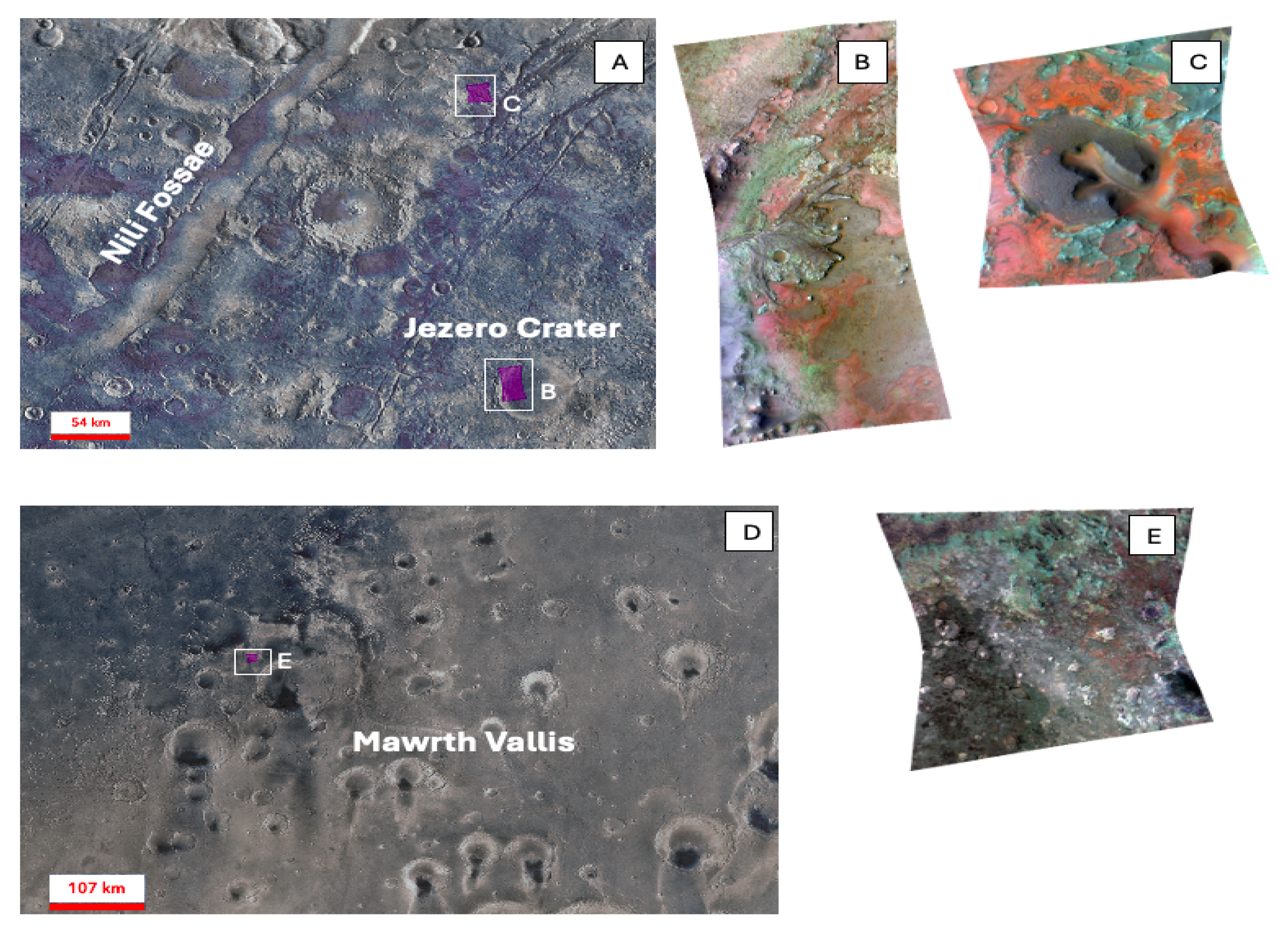
Initially, the region of the Jezero Crater is analyzed, which has been studied by Pletl et al. [9] and Gao et al. [10]. To evaluate the clustering performance, we apply two established internal validation metrics commonly used in unsupervised learning: the Calinski–Harabasz (CH) index [38] and the Davies–Bouldin (DB) [39] index. These metrics quantify the quality of a clustering result based on intra-cluster compactness and inter-cluster separation. The CH index yields higher values when clusters are dense and well-separated [38], whereas the DB index penalizes overlapping or poorly separated clusters, with lower values indicating better validity [39].

To make an evidence-based conclusion, we follow the approach of Pletl et al. [9]. In this study, the average values of the metrics across all examined cluster numbers are calculated. This is done to mitigate fluctuations in the metric values. The results are presented in

Table 1. Mean value of the CH and DB indices and the silhouette score. All values are based on results obtained using a cluster count ranging from 5 to 20. The analyzed region corresponds to the Jezero HRL000040FF dataset. Values in parentheses indicate the change relative to the value of the previous pipeline option.

Methods	Silhouette Score	Calinski–Harabasz	Davies–Bouldin
Pletl et al. [9]	0.380	114,928	0.818
UMAP + k-Means	0.410 ($\Delta$ +7.9%)	123,123 ($\Delta$ +7.1%)	0.781 ($\Delta$ −4.5%)
UMAP + k-Means + filter	0.453 ($\Delta$ +10.5%)	125,275 ($\Delta$ +1.7%)	0.8036 ($\Delta$ +2.9%)

.

According to all three indices, the UMAP algorithm with optimized parameters outperforms the reference method. The application of the stripe filter leads to improvements in two of the evaluated metrics, while a negative effect is observed in the DB metric, indicating that the overall contribution of the filter is rather minor. Nevertheless, the combination of optimized UMAP parameters and the filter suggests a generally more robust clustering performance, although the impact of each individual component may vary depending on the dataset. Since this configuration produces the optimal values for the Jezero region, subsequent analyses are carried out with the stripe filter applied. In the next step, a Silhouette plot is analyzed to evaluate the method’s ability to identify the optimal number of clusters. Once again, the results are compared with those reported by Pletl et al. [9].

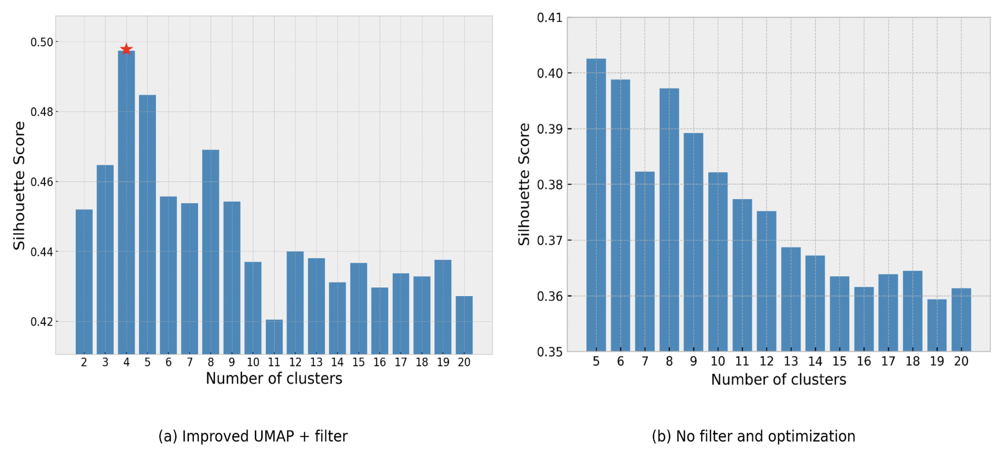
For this purpose, the SC values are plotted against the number of clusters. In Figure 3a, the silhouette coefficient reaches a peak of 0.50 at four clusters, suggesting that this configuration provides the most coherent and well-separated groupings in the dataset. In contrast, the reference results by Pletl et al. [9], shown in Figure 3b, exhibit generally lower SC values across all tested cluster numbers, with a maximum value that remains below 0.45. The overall range of SC values in the optimized pipeline lies between 0.42 and 0.50, which consistently surpasses the previous benchmarks. This indicates that the combination of parameter tuning in UMAP and the application of the stripe correction filter not only improves clustering compactness but also enhances inter-cluster separability. Additionally, the automated process successfully identifies the optimal cluster count based on the defined SC-based evaluation metrics, eliminating the need for manual interpretation of plots. These results suggest a more reliable clustering outcome, particularly for geologically complex regions like Jezero Crater.

As the next step, a qualitative analysis will be conducted in addition to the quantitative evaluation. For this purpose, the minerals extracted from the SCM are compared with an expert map.

To assign a mineral label to a class, a representative mean spectrum for that class is first calculated. In the initial step, all pixels are grouped according to the their classes C. For each wavelength band $\lambda$, the pixel values are summed, and the average value is calculated. Subsequently, the resulting spectrum is compared with a reference spectrum. These reference spectra are sourced from a library specifically created for CRISM data, provided by Ehlmann et al. [40]. The assignment of an mean spectrum to a representative mineral is performed by evaluating the numerical similarity with each spectrum stored in the database. The reference spectrum with the highest similarity is classified as the identified mineral. To quantify the numerical similarity between spectra, the spectral angle is calculated. This metric is commonly used in the comparison of hyperspectral images and is described by Agarla et al. [41]. Using Equations (13) and (14), the spectral angle APPSA is calculated, aiming for minimal values to indicate a high degree of similarity and lower error.

$$\rho =arccos\left({\displaystyle \frac{{\sum }_{i=1}^p\left({\mathbf{I}}_i^{*}·{\mathbf{I}}_i\right)}{\sqrt{{\sum }_{i=1}^p\left({\mathbf{I}}_i^{*}·{\mathbf{I}}_i^{*}\right)}·\sqrt{{\sum }_{i=1}^p\left({\mathbf{I}}_i·{\mathbf{I}}_i\right)}}}\right)$$

(13)

$$\mathrm{APPSA}={\displaystyle \frac{1}{m\times n}}{\mathbf{1}}^T\rho \mathbf{1}$$

(14)

Here, m and n denote the number of pixels in the horizontal and vertical directions, respectively, while p represents the number of spectral channels. ${\mathbf{I}}_i^{*}$ and $I_i$ refer to the reference spectrum and the average spectrum of a class, respectively. By applying the comparison to an image consisting of a single pixel, this metric can be effectively utilized to align the two spectral profiles.

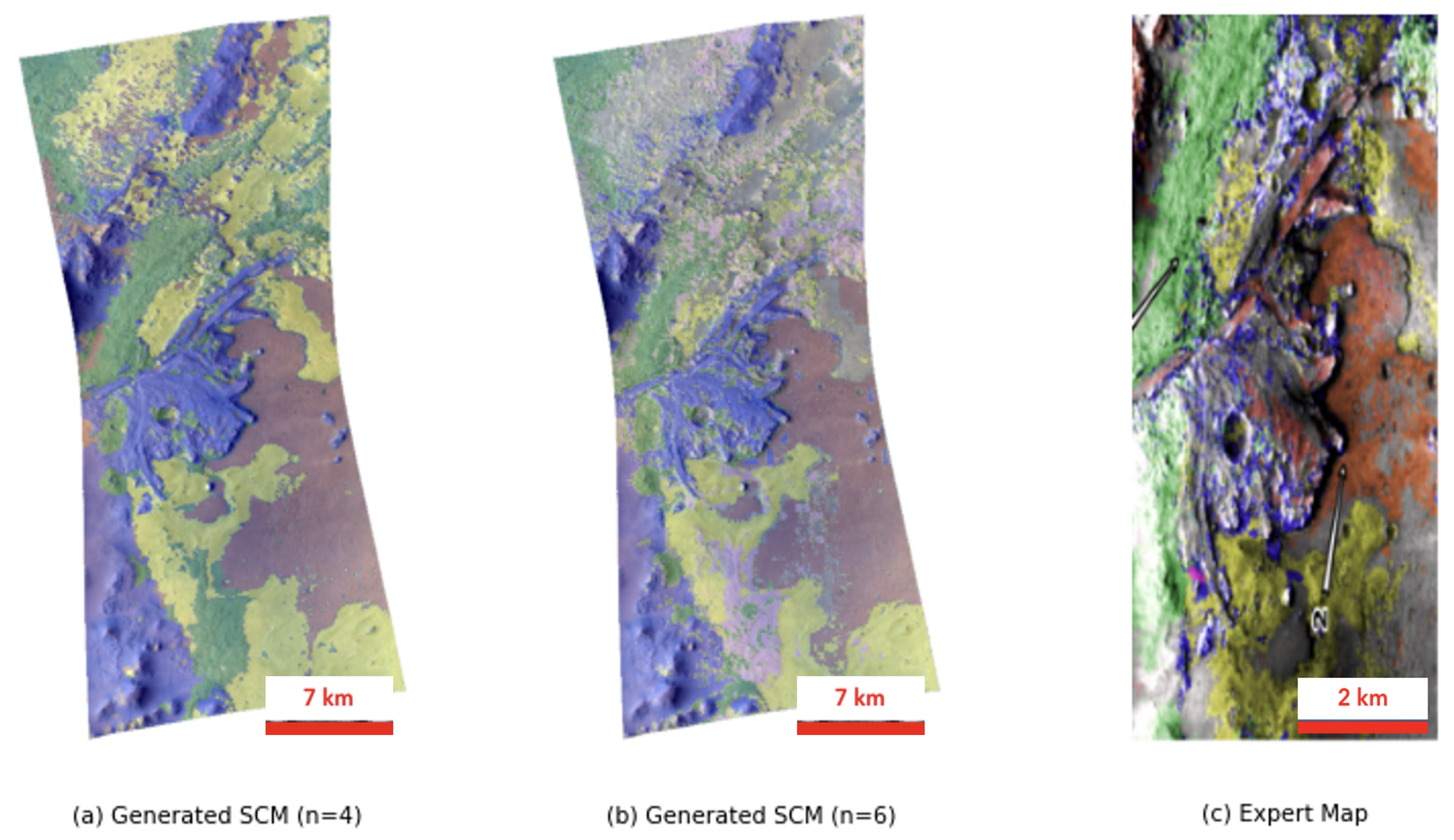
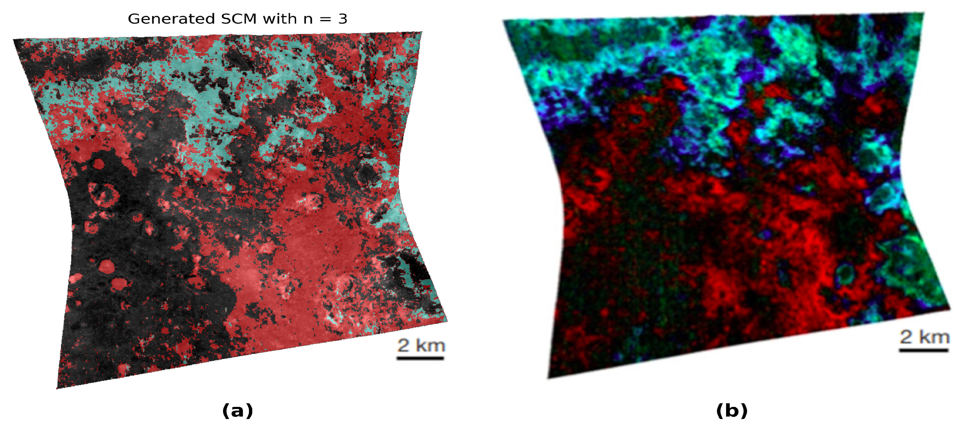
The expert map, which is used for comparison is provided by Gao et al. [10]. It contains a total of six different classes, five of which are associated with minerals, complemented by an unclassified category. To ensure an accurate assessment of the post-processing performance, the comparison is conducted using the previously identified optimal number of four clusters. And additionally, an SCM generated analogously to [10] using six clusters is shown for comparison in Figure 4.

The resulting class labels for (a) are listed in the

Table A2. Results of the HRL000040FF dataset for mineralogy after matching the mean spectra with the CRISM database. Entries listed higher within a column indicate a greater similarity with the reference spectra.

Source	Class 1	Class 2	Class 3	Class 4
Gao et al. [10]	Olivine	Carbonate	Pyroxene	Smectite
	Fe-Olivine	Mg-Carbonate	LC-Pyroxene	$H_{2}O$-Ice
	Mg-Olivine	Kaolinite	$H_{2}O$-Ice	$C{O}_2$-Ice
Spectral library	Mg-Carbonate	Mg-Olivine	$C{O}_2$-Ice	Gypsum
	Chloride	Alunite	Chloride	LC-Pyroxene
	Al-Smectite	Al-Smectite	Feldspar	Fe-Sulfate

in descending order of their similarity. An analysis of the results for (a) reveals a significant overlap between the classification based on the database comparison and the expert assessment. For classes 1 to 3, the identified minerals align with the expert interpretation. Notably, in class 1, both iron- and magnesium-rich olivines are identified. However, for class 4, the mineral smectite is not among the five minerals with the highest similarity.

The second region analyzed is the FRT0000AA7D dataset from the Mawrth Vallis region, which was previously studied by Bishop et al. [42]. As previously noted, the availability of expert maps is limited. Consequently, no reference values for the clustering metrics are available for this region. To enable evaluation of the pipeline in this region, we first compute the metrics without applying UMAP optimization or the stripe filter. Subsequently, the impact of these two modifications is calculated analogously to the Jezero region, as summarized in

Table 2. Mean value of the SC, CH and DB indices. Both values are based on results obtained using a cluster count ranging from 2 to 20. The analyzed region corresponds to the Mawrth Vallis FRT0000AA7D dataset. Values in parentheses indicate the change relative to the value of the previous pipeline option.

Methods	Silhouette Score	Calinski–Harabasz	Davies–Bouldin
Baseline	0.391	203,119	0.817
UMAP + k-Means	0.406 ($\Delta$ +3.8%)	189,175 ($\Delta$ −6.9%)	0.814 ($\Delta$ +0.4%)
UMAP + k-Means + filter	0.365 ($\Delta$ −10.1%)	248,171 ($\Delta$ +31.2%)	0.836 ($\Delta$ −2.7%)

.

In contrast to the Jezero region, using the optimized UMAP parameters did not result in a clearly pronounced performance improvement. Although higher values were achieved for two of the metrics, the CH index decreased. The effect of applying the stripe filter is particularly noteworthy. While the CH value increased considerably in this case, the crucial SC value dropped significantly, and the DB value decreased slightly. This indicates that the application of the stripe correction filter can also have a negative impact on cluster performance. A method for controlling the application of the stripe filter is discussed in Section 3.2 based on a global analysis. Since the application of the optimized UMAP parameters without the stripe filter yields the best results, the following qualitative analysis is conducted using these settings.

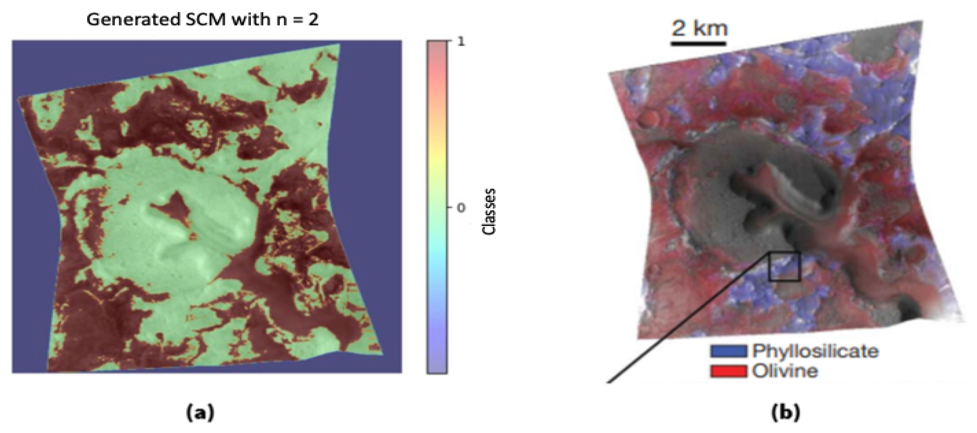
In the qualitative analysis, the generated SCM shown in Figure 5 exhibits strong visual agreement with a reference map provided by [42]. The results of the mineralogical database comparison are again summarized in

Table A3. Results of the FRT0000AA7D dataset for mineralogy after matching the mean spectra with the CRISM database. Entries listed higher within a column indicate a greater similarity with the reference spectra.

Source	Class 1	Class 2	Class 3
Bishop et al. [42]	Fe/Mg-smecitite	Al-phyllosilicates	Poorly crystalline aluminosilicates
	Fe-Olivine	Alunite	$C{O}_2$-Ice
	Mg-Olivine	Kaolinite	$H_{2}O$-Ice
Spectral library	Chloride	Mg-Carbonate	Gypsum
	Mg-Carbonate	Gypsum	LC-Pyroxene
	Al-Smectite	Fe-Sulfate	Fe-Sulfate

. In addition to these visual correspondences, mineralogical overlaps are also apparent. For the class that appears in red in the expert map and is labeled as Fe/Mg-smectite, the database comparison identifies Al-smectite as well as a dominance of Fe/Mg-olivines. This likely indicates either a mixed mineralogy (smectite + primary silicates + evaporites) or spectral misclassification within the SCM. The turquoise class, which the expert interprets as Al-phyllosilicates, corresponds well with the database results yielding alunite and kaolinite. Additional minerals such as Mg-carbonate, gypsum, and Fe-sulfates suggest associated carbonates, evaporites or secondary sulfates. The greenish class of poorly crystalline aluminosilicates is largely associated with the black class of the SCM.

However, the corresponding black class in the expert map was not subjected to mineralogical interpretation, making a definitive assessment difficult. These discrepancies highlight a limitation of a purely database-driven mineralogical interpretation. Alternative approaches that could be implemented in future work are hence discussed in Section 4.

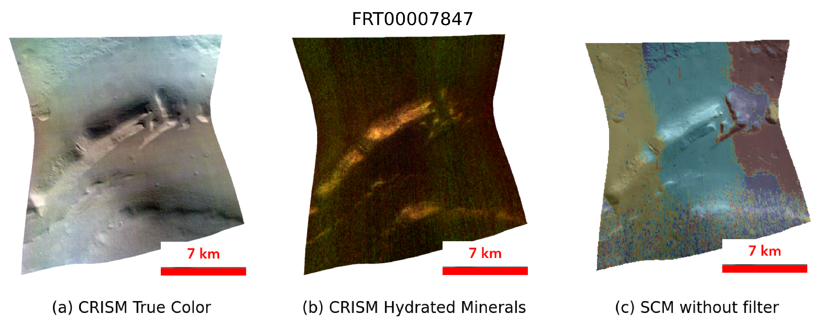
The third region analyzed is an area within Nili Fossae, using the FRT00003E12 dataset. As a reference, a map based on mineral indicators, created according to [18] and published by Mustard et al. [43], is utilized. This region presents a particular challenge because, unlike the previously analyzed areas, it predominantly consists of only two distinct mineralogical components.

Analogous to the Mawrth Vallis region, no quantitative comparison is available for this area, a baseline value without UMAP optimization and without the application of the stripe filter is determined first. The corresponding results are presented in

Table 3. Mean value of the SC, CH and DB indices. Both values are based on results obtained using a cluster count ranging from 2 to 20. The analyzed region corresponds to the Nili Fossae FRT00003E12 dataset. Values in parentheses indicate the change relative to the value of the previous pipeline option.

Methods	Silhouette Score	Calinski–Harabasz	Davies–Bouldin
Baseline	0.388	219,905	0.831
UMAP + k-Means	0.420 ($\Delta$ +8.2%)	263,466 ($\Delta$ +19.8%)	0.809 ($\Delta$ −2.6%)
UMAP + k-Means + filter	0.412 ($\Delta$ −1.9%)	163,466 ($\Delta$ −54.7%)	0.809 ($\Delta$ +0.0%)

and show a similar pattern to the two previously analyzed regions. Here as well, the usage of the UMAP parameters leads to a partly significant improvement across all clustering metrics. Of particular note is the comparatively strong increase in the SC value. When applying the stripe filter, however, a deterioration in clustering performance is observed for the Nili Fossae region. While the SC and CH parameters decrease considerably in some cases, the DB value shows at least a stagnation rather than a decline. Overall, the results confirm the general trend that UMAP optimization tends to have a positive effect on clustering performance, whereas the application of the stripe filter exerts a rather negative influence.

Since a quantitative analysis of this region has not been conducted so far, the assessment is based solely on comparing the two mineralogical maps, which are shown in Figure 6. Additionally, it draws on the mineralogical interpretation of the SCM by comparing it with the spectral library, as summarized in

Table A4. Results of the FRT00003E12 dataset for mineralogy after matching the mean spectra with the CRISM database. Entries listed higher within a column indicate a greater similarity with the reference spectra.

Source	Class 1	Class 2
Mustard et al. [43]	Phyllosilicate	Olivine
	$H_{2}O$-Ice	Fe-Olivine
	$C{O}_2$-Ice	Mg-Olivine
Spectral library	Gypsum	Mg-Carbonate
	LC-Pyroxene	Chloride
	Fe-Sulfate	Al-Smectite

. Particularly noteworthy is the class highlighted in both representations by a reddish coloration. Here, there is a high degree of agreement between the SCM and the reference map, with even fine structural details aligning in both. Furthermore, comparison of the representative mean spectrum with the spectral library suggests that iron- and magnesium-rich olivines exhibit the greatest similarity. For the second class, however, the database comparison does not provide a correct identification, and slight discrepancies in the cluster structures between the two maps can be observed. While phyllosilicates were identified by the author, the database comparison instead yields ices and gypsum as the minerals with the highest spectral similarity. This could be attributed to the spectral resemblance of the materials. Nonetheless, aside from a few inconsistencies in the central region, the SCM replicates these structures in a relatively congruent manner. The discrepancy in the central region may be attributable to the fact that, unlike the clustering approach, mineral indicators need not provide complete coverage of the area.

3.2. Evaluation of the Stripe Filter Approach

In this section, we evaluate the capability of UMAP and k-means, in combination with a striping filter, to robustly cluster regions of the Martian surface. This approach is particularly relevant because it is intended to form the basis for a fully automated process.

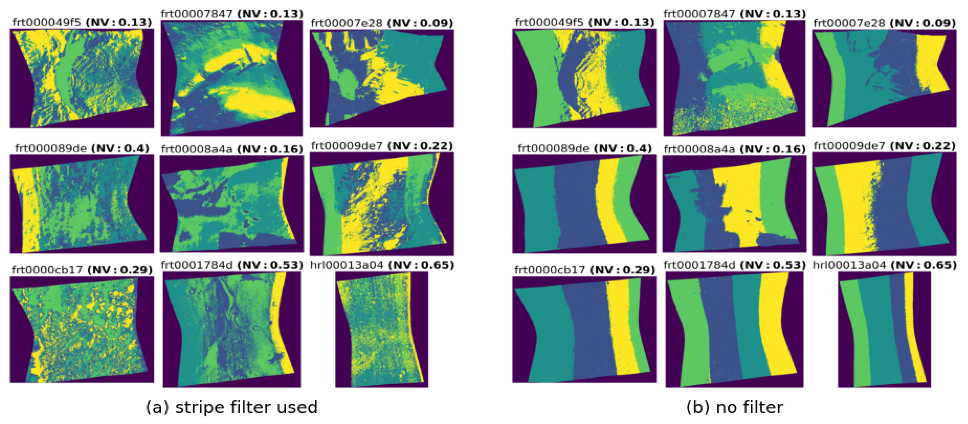
As shown in Figure 7b, many regions exhibit vertically oriented striping patterns in their clustering results. The intensity of these patterns ranges from purely vertical stripes to mixed forms in which additional cluster structures can be observed. These outcomes arise when the previously described clustering procedure is conducted without using the striping filter.

On the left side of Figure 7a, the results after applying the striping filter are shown. Notably, each region displays a significant degree of improvement after applying the striping filter. In several cases, the filter effectively fully reduces the dominance of vertical artifacts and allows cluster boundaries to emerge more clearly, particularly in regions where mixed cluster structures were previously obscured. Although the maps differ in the extent to which striping is reduced, the patterns become more interpretable. The remaining variations points to a dataset-dependent filter performance and emphasizes the need for a quantitative criterion to assess its effectiveness.

To assess whether the noise level in a dataset can be effectively handled by the striping filter, we used the noise_variance_ attribute from the scikit-learn PCA implementation [44]. This method follows the probabilistic interpretation of PCA by Tipping and Bishop [45]. The attribute estimates the isotropic noise before filtering. Conventional clustering metrics are unsuitable for this purpose, as the resulting stripes, while visually appearing as compact clusters, are mineralogically meaningless. If the noise level exceeds a defined threshold, the filter is unlikely to produce substantial improvements.

As established in Section 3.1, the use of the filter may be unnecessary and could even reduce the performance of the clustering process. For this reason, it is beneficial to establish a quantitative threshold value that indicates whether the application of the stripe correction filter is warranted. Furthermore, a threshold can be defined above which the clustering results are likely to be affected by residual stripe artifacts, potentially leading to erroneous classifications.

To determine such thresholds, a test dataset comprising 25 regions representing diverse Martian surface types was analyzed, and the noise variance was computed for each region. The regions and their corresponding values are listed in Table A5 in the Appendix. Furthermore, these regions are classified into three different classes according to the filter efficiency as follows.

Class 1 includes regions that do not exhibit any stripe artifacts during clustering even without applying the filter. Among these are, for instance, the regions examined in Section 3.1. Class 2 contains those regions that initially show stripe artifacts but can be corrected by applying the filter. This also includes regions in which minimal residual artifacts remain (see FRT00008A4A in Figure 7). Class 3 considers regions that still display significant residual artifacts even after applying the stripe filter. An example of this is the dataset FRT0001784D.

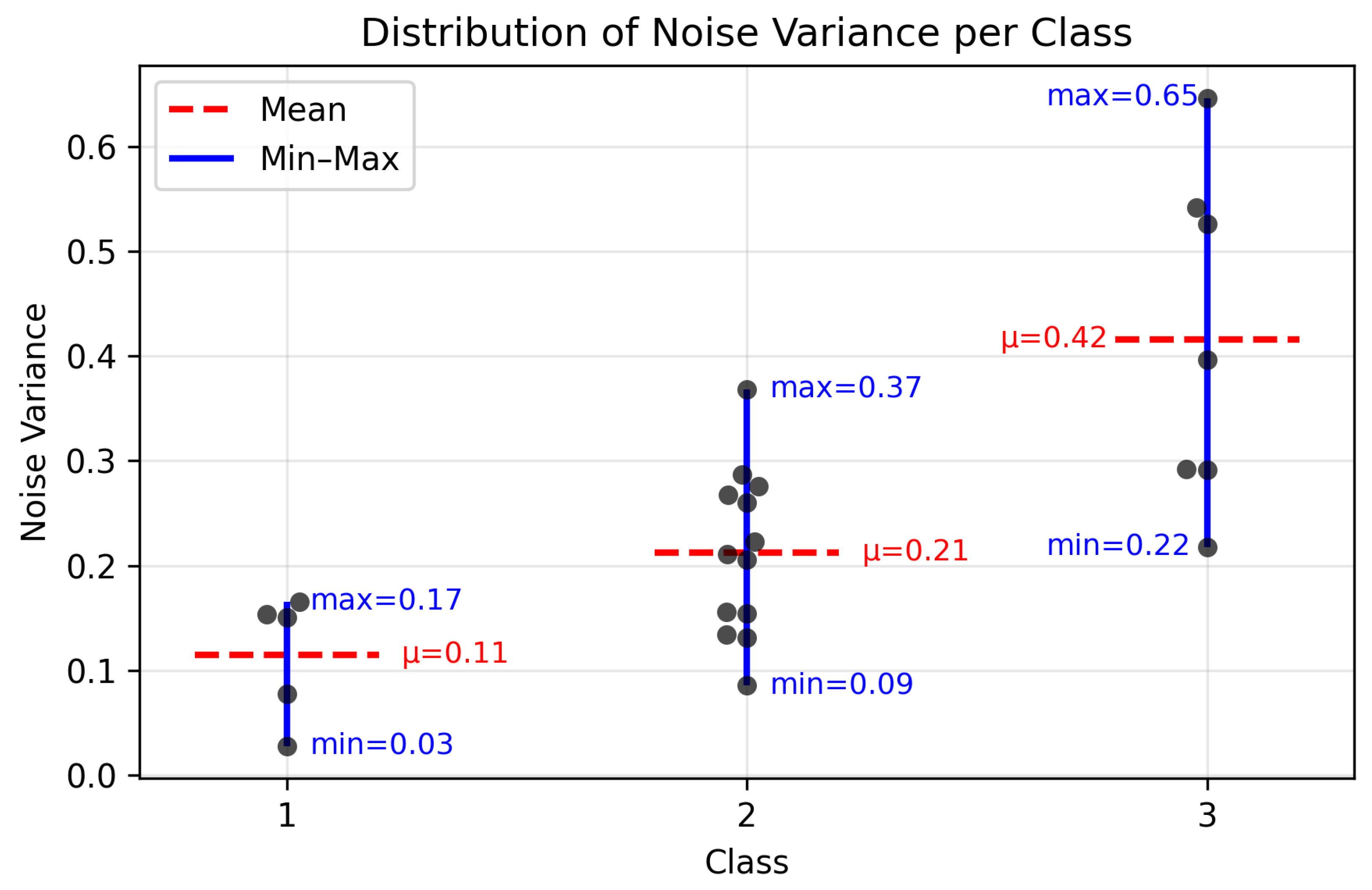
For determining a threshold value for the application of the filter, the distributions of classes 1 and 2 are examined, as shown in Figure 8. Class 1 shows relatively low and consistent noise variance values, while class 2 exhibits a higher mean noise variance and a wider spread, suggesting increased variability among datasets. The upper limit of class 1 (0.17) overlaps with the lower limit of class 2 (0.09). This overlap is not undesirable, as it reflects the natural variability of CRISM observations and suggests that the threshold between low and moderate noise levels is continuous rather than discrete. Since, however, the effects of omitting the filter for class 2 regions are more severe than the redundant application of the filter to class 1 regions, a value close to the minimum of class 2 is preferred. Based on the examination of both point distributions, a value of 0.10 is therefore proposed as the threshold for filter application and is integrated into our framework. In general, all regions exceeding this value are processed using the filter.

The second threshold is intended solely as additional information for the user, serving as an indicator of potentially compromised clustering results that may require manual inspection. For this purpose, the class boundaries between classes 2 and 3 are again analyzed. It is observed that class 3 exhibits a much broader distribution, whereas class 2 is more compactly distributed around a mean value of 0.21. Considering the point distributions, it is proposed that clustering results may become unreliable when the noise variance exceeds a threshold of 0.40. Since this threshold serves only an informative purpose, it is chosen to be higher than the maximum value of class 2 and close to the mean of class 3.

In summary, the filter yields artifact-free clustering results in 18 out of 25 regions $(72\%)$, demonstrating a high level of robustness across diverse datasets. Moreover, it almost completely corrects artifacts in 13 out of 20 affected regions $(65\%)$. Only 7 regions continue to exhibit more pronounced artifacts. However, even in these cases, the resulting cluster structures remain sufficiently coherent to enable at least partial interpretation. Overall, the filtering procedure can therefore be considered effective, with potential for further improvement particularly in regions exhibiting threshold values above 0.40, where additional refinements may enhance performance.

4. Discussion

The results of this study demonstrate that the proposed pipeline, combining optimized UMAP parameters, k-means clustering, and an adaptive stripe correction filter, consistently improves clustering performance for CRISM hyperspectral data compared to previous approaches. Across multiple regions, the method achieved higher CH values, lower DB scores and improved silhouette coefficients. Closer inspection indicate that UMAP optimization provides the most consistent improvements across all datasets, while the adaptive stripe filter, when guided by the proposed noise-variance thresholds, enhances robustness and reproducibility in the proposed pipeline. In the Jezero region, the automated clustering process successfully identified the optimal cluster number without manual intervention.

The comparison with expert maps, such as the classification by Gao et al. [10], showed substantial agreement, particularly in Jezero and Mawrth Vallis. The spectral library matching further supports the mineralogical interpretations. Minor discrepancies between database and expert classifications primarily occur where spectral features overlap or are weakly expressed.

The global evaluation of the adaptive stripe correction filter reveals that its impact is dataset-dependent. Although the filter is designed to remove primarily stripe related noise in a specific image direction while preserving genuine scene information, the balance between instrumental noise and true geological signal varies across regions. In datasets where the spatial pattern or intensity of striping partially overlaps with, or visually resembles, real mineralogical gradients, the adaptive filter may inadvertently suppress meaningful spectral–spatial variability. This effect might be particularly evident in the Mawrth Vallis region, where higher overall noise variance and heterogeneous spectral characteristics increase the risk that the filter removes genuine mineralogical information together with the striping. For Nili Fossae, however, the situation is different. The noise variance for this region is very low (0.0277), indicating that the dataset contains minimal striping and is already of high quality. Applying the destriping filter under these conditions provides no corrective benefit and can instead introduce small distortions into an otherwise clean dataset. A detailed quantification of these effects and potential strategies to mitigate unintended information loss represent possible directions for future methodological development.

In Jezero, the filter improves clustering metrics, whereas in Mawrth Vallis and Nili Fossae, its effect is less pronounced or occasionally negative. A probabilistic PCA-based analysis of 25 CRISM regions demonstrates that these variations can be predicted from the estimated noise variance, allowing objective control of filter application. Three classes of filter efficiency were identified, from artifact-free to residual-affected, leading to the definition of two practical thresholds, above which the filter should be applied and beyond which clustering results may require manual inspection. Using these thresholds, the filter produced artifact-free clustering in 18 out of 25 regions. This represents a clear improvement of the overall processing pipeline, as it enables meaningful clustering for the majority of regions that would otherwise remain partially or completely unanalyzable.

These findings suggest that the combination of parameter tuning in UMAP and the use of the stripe filter not only increases intra-cluster compactness but also enhances inter-cluster separability. After a comprehensive parameter sweep on the Jezero dataset, the resulting configuration was fixed for the entire pipeline, as it provided the best overall improvement in cross-regional performance. Although minor site-specific tuning could further improve local performance, initial trade-off analyses indicated that a unified configuration offers a robust balance between adaptability and automation. Datasets that could not be effectively corrected by the stripe filter exhibited high noise variance values, indicating that excessive isotropic noise limits filter performance. This relationship highlights the potential of noise variance as a predictive metric for filter applicability in our proposed framework.

A major strength of the presented approach lies in its full integration of preprocessing, dimensionality reduction, clustering, and evaluation into a single, reproducible pipeline. By combining statistical cluster validation with spectral library matching, the method provides both quantitative performance metrics and interpretable mineralogical outputs. Additionally, the approach proved to be robust across geologically diverse regions, suggesting that it can be applied to a wide range of CRISM datasets.

Despite these advantages, several limitations remain. Extending the proposed pipeline to global-scale CRISM data presents additional computational challenges due to the volume and variability of hyperspectral observations. Efficient large-scale implementation will require strategies such as distributed or parallelized processing, spatial data partitioning, and incremental model updates to manage memory load and ensure consistent clustering across regions. Beyond computational scalability, there are additional challenges related to the spatial heterogeneity of data quality, variable illumination geometry, atmospheric conditions, and the need for consistent clustering across independently processed regions. Addressing these issues might require adaptive preprocessing, photometric normalization, and a harmonization step to align cluster definitions between tiles. Moreover, large-scale validation efforts using complementary datasets and distributed processing frameworks will be essential to ensure the accuracy and coherence of a global mineralogical atlas of Mars.

Furthermore, challenges persist in achieving a fully automated, globally consistent clustering framework. The noise-variance threshold, estimated using PCA, provides a quantitative measure for assessing data quality and potential limitations of the stripe filter. Another limitation arises from the use of conventional spectral similarity metrics, which may struggle to distinguish minerals when diagnostic absorption features overlap or are weakly expressed. This challenge is compounded by the limited number of Mars-relevant spectra currently available in reference libraries, which can restrict classification accuracy. Complementary approaches such as multispectral or hyperspectral data fusion and deep-learning-based feature extraction hold strong potential to overcome these limitations by capturing subtle, non-linear spectral relationships. These methods, however, are inherently complex and will require dedicated investigation. Their refinement and integration within the proposed pipeline are clearly necessary but lie beyond the scope of the present study and will be addressed in future work.

In this sense, the implications for planetary-scale analysis lie not in immediate global deployment but in establishing the methodological basis and computational strategies required to achieve it in future work. The framework offers a scalable analysis pipeline for generating spectral cluster maps, which could support future mapping campaigns, landing site selection, and in situ exploration planning and hence could have direct implications for large-scale planetary surface analysis. Furthermore, the ability to match cluster spectra with reference libraries enables semi-automatic mineral identification at regional scales, reducing the need for extensive manual interpretation.

Future work should therefore focus on refining the noise variance threshold to better predict filter performance prior to processing, enabling the automated exclusion or flagging of datasets with noise levels too high for effective correction. Additional improvements could include the integration of adaptive filtering techniques, the exploration of alternative modern dimensionality-reduction algorithms, and the evaluation of hybrid clustering strategies. Expanding the spectral library with further Mars-relevant mineral signatures would also increase classification accuracy and support more comprehensive mineralogical interpretation. Moreover, future efforts should integrate these methodological and computational optimizations, such as distributed or parallelized processing, to enable efficient large-scale application of the pipeline. Ultimately, these developments will be crucial steps toward fully automated, global-scale CRISM data analysis and the generation of coherent, high-resolution mineralogical maps of the Martian surface.

5. Conclusions

This study presents the basis for a fully automated and reproducible framework for processing CRISM hyperspectral data. The proposed data and model pipeline substantially reduces manual intervention, enhance reproducibility, and improve the reliability of spectral cluster maps derived from CRISM data. Across multiple test sites, including Jezero Crater, Nili Fossae, and Mawrth Vallis, the optimized pipeline consistently outperformed previous approaches in internal validation metrics and produced mineralogical maps in good agreement with expert classifications.

Its modular design allows for future extensions, including distributed or parallelized processing for global-scale applications, integration of adaptive filtering techniques, and expansion of spectral libraries with additional Mars-relevant mineral signatures. In combination with complementary approaches such as multispectral data fusion and deep-learning-based feature extraction, this could enhance mineral discrimination and improve automatic mineral mapping.

In summary, this study demonstrates that automation, when combined with rigorous quantitative evaluation and noise-aware filtering, can significantly advance hyperspectral mineralogical mapping on Mars. The framework offers a scalable and interpretable foundation for large-scale geospatial analysis, supporting future mapping campaigns, landing site assessment, and in situ exploration planning, and thus represents a crucial step toward the comprehensive mineralogical characterization of the Martian surface.