Article

Optical Remote Sensing Ship Detection Combining Channel Shuffling and Bilinear Interpolation

College of Field Engineering, Army Engineering University of PLA, Nanjing 210007, China
*
Author to whom correspondence should be addressed.
Remote Sens. 2025, 17(23), 3828; https://doi.org/10.3390/rs17233828
Submission received: 17 October 2025 / Revised: 19 November 2025 / Accepted: 24 November 2025 / Published: 26 November 2025

Highlights

What are the main findings?
  • The maritime ship targets suffer from the problem of imbalanced length-to-width ratios, which can lead to a decrease in detection accuracy.
  • The sea wave background of maritime ships, as well as the similar color between ships and seawater, can blur the edge information of ships, thereby increasing the miss rate.
What are the implications of the main findings?
  • To address the issue of imbalanced length-to-width ratios, this paper designs a loss function that combines position, shape, and scale information, and validates the effectiveness of the method through various experiments.
  • To address the problem of ship edge information being easily confused with seawater and other background information, a feature enhancement module and an edge-gated upsampling module are designed. These modules enhance ship feature information and suppress background information, thereby reducing the miss rate.

Abstract

Maritime remote sensing ship detection has long been plagued by two major issues: the failure of geometric priors due to the extreme length-to-width ratio of ships; and the sharp drop in edge signal-to-noise ratio caused by the overlapping chromaticity domain between ships and seawater, which leads to unsatisfactory accuracy of existing detectors in such scenarios. Therefore, this paper proposes an optical remote sensing ship detection model combining channel shuffling and bilinear interpolation, named CSBI-YOLO. The core innovations include three aspects: First, a group shuffling feature enhancement module is designed, embedding parallel group bottlenecks and channel shuffling mechanisms into the interface between the YOLOv8 backbone and neck to achieve multi-scale semantic information coupling with a small number of parameters. Second, an edge-gated upsampling unit is constructed, using separable Sobel magnitude as structural prior and a learnable gating mechanism to suppress low-contrast noise on the sea surface. Third, an R-IoU-Focal loss function is proposed, introducing logarithmic curvature penalty and adaptive weights to achieve joint optimization in three dimensions: location, shape, and scale. Dual validation was conducted on the self-built SlewSea-RS dataset and the public DOTA-ship dataset. The results show that on the SlewSea-RS dataset, the mAP50 and mAP50–95 values of the CSBI-YOLO model increased by 6% and 5.4%, respectively. On the DOTA-ship dataset, comparisons with various models demonstrate that the proposed model outperforms others, proving the excellent performance of the CSBI-YOLO model in detecting maritime ship targets.

1. Introduction

With the development of optical remote sensing technology [1,2,3,4,5,6], object detection based on various tasks has also made significant progress. Many dangerous tasks that were previously performed manually can now be replaced by machines. Tasks such as fire monitoring [7,8] and security duties [9,10] can be entirely dependent on remote sensing and object detection technologies. However, in some complex environments, the performance of object detection is not satisfactory. For example, in maritime ship detection, ships are different from other targets such as vehicles, aircraft, and buildings. Ships are targets with an imbalanced length-to-width ratio. From the top-down perspective of remote sensing, the dark seawater becomes the background information for ship detection. The waves on the sea and the changing color of the seawater with sunlight can cause significant difficulties in the detection and localization of maritime ships. Therefore, research on ship detection in such complex scenarios is a meaningful challenge.
Deep learning techniques have gained widespread application due to their ability to learn effective feature information from the given data. According to the mainstream classification method for object detection, detectors can be divided into two-stage detectors and one-stage detectors. The computational process of two-stage detectors involves first proposing candidate boxes and then classifying and regressing these boxes. For example, R-CNN [11] uses selective search to generate candidate boxes and was the first to introduce CNN features into detection. Subsequently, Faster R-CNN [12] replaced selective search with a Region Proposal Network, and Mask R-CNN [13] added a mask branch and replaced ROI Pooling with bilinear interpolation. Although their detection accuracy has been continuously improving, they are not memory-efficient and cannot meet real-time requirements. This has laid the foundation for the rise of one-stage detectors. One-stage detectors can directly predict classes and regress on the feature map without the need to generate candidate boxes. When it comes to one-stage detectors, the YOLO series cannot be overlooked. Since YOLOv1 [14] was introduced in 2015, it was the first to regard detection as a regression problem, with a computational speed far exceeding that of two-stage detection models. However, its performance in detecting small objects was very disappointing. YOLOv2 [15] learned from experience, introduced Anchor and multi-scale training to address the shortcomings of the first generation, achieving both speed and accuracy. YOLOv3 [16] built on the previous work by introducing a feature pyramid for multi-scale prediction and residual connections, further optimizing the detection of small objects. YOLOv4 [17] continued to improve, with increased accuracy in detecting small objects and enhanced performance in multi-scale target detection. YOLOv5 introduced five versions (n, s, m, l, x), restructured the loss and optimization functions, and improved the detection capability for occluded objects. Subsequent versions, YOLOv6 [18] and YOLOv7 [19], made further improvements and optimizations. YOLOv8 [20], the latest in the series, restructured the network architecture, removed Anchor, used decoupled heads, and unified the tasks of detection, segmentation, and pose estimation. It is currently one of the most popular, widely used, and stable detection models, with performance in many scenarios even surpassing the later versions of YOLOv9 [21], YOLOv10 [22], and YOLOv11 [23].
Traditional YOLO detection models can still ensure effectiveness when facing general detection tasks, but in some harsh environments, detection accuracy drops sharply. Therefore, many scholars have improved the basic model in their respective challenging fields to make it work in special environments. Hu et al. [24] addressed the issue of small target responses being easily overshadowed by using a cascaded feature suppression module and a feature enhancement module. They employed the idea of cross-layer subtraction and a dual-branch downsampling followed by fusion strategy to suppress large target features and improve the signal-to-noise ratio of small targets. Xie et al. [25] introduced an attention module, designing the Micro-Attention Module (MAM), which uses multi-branch depthwise separable convolution combined with Inception-style convolution and Squeeze-and-Excitation lightweight attention mechanisms. This module recalibrates targets in complex environments from both channel and spatial dimensions and amplifies effective channel responses using exponential weighting, significantly suppressing the noise of water reflection and ripples in water surface detection tasks. Furthermore, Tang et al. [26] cascaded channel attention and spatial attention to recalibrate the background suppression and target enhancement before the feature map enters the neck network, alleviating the interference of complex backgrounds. Chen et al. [27] not only designed an attention module but also combined Position Memory Enhanced Self-Attention (PMESA). They replaced the traditional Bottleneck with a Retentive Block in the C2f bottleneck, embedding Manhattan distance-encoded relative position memory. This allows self-attention to explicitly model while computing feature similarity, thereby suppressing background noise and enhancing semantic consistency in occluded areas. The above scholars have made professional designs and improvements for various complex scenarios, including small targets, multi-angle views, occluded targets, and external factors such as water surface reflection. Therefore, after considering the research of predecessors and combining the actual needs of this paper’s task, the CSBI-YOLO model was designed. The challenges addressed are the similarity and mixture of maritime ship targets with seawater background, as well as the imbalance of the ship targets’ aspect ratio. The following three improvement strategies were designed:
  • A feature enhancement module was designed to reconstruct inter-group interactions through channel shuffling. Parallel branches capture local textures and global contexts separately, and adaptive weighting is performed in the channel dimension. This simultaneously enhances fine-grained features and long-range dependencies, achieving significant accuracy gains at the cost of a small number of parameters.
  • This paper proposes the Edge-Gated Upsampler, which first generates an edge confidence map using the Sobel operator and then dynamically adjusts the edge branch weights through a temperature-learnable gating mechanism. This is done in parallel with the interpolation branch to achieve adaptive trade-offs between structural details and smooth regions, effectively enhancing the network’s ability to discriminate narrow targets.
  • A logarithmic-power composite transformation of the IoU between the predicted box and the ground-truth box is introduced to construct the R-IoU-Focal Loss. This maps the regression difficulty to exponential weights, enabling the network to focus on narrow targets with low IoU. In the complex maritime ship detection task, this loss significantly improves localization accuracy and robustness, providing a new optimization paradigm for the detection of narrow and low-contrast targets.

2. Relate Work

2.1. Imaging Technology for Remote Sensing Ship Detection

Remote sensing ship imaging can be divided into three major branches: optical imagery, synthetic-aperture radar (SAR) imagery, and infrared imagery. The differences in spectral frequency bands determine the key considerations in designing the corresponding detection models. Below, we introduce the three imaging technologies.

2.1.1. Optical Remote Sensing Ship Detection

Visible light is a near-infrared wave that relies on solar irradiance. This type of light can help the model automatically learn the differences between the ship’s body and the background. However, there are obvious drawbacks. Due to the influence of lighting conditions, the results can vary significantly across different seasons, sea conditions, and even different times of the same day. Additionally, cloud cover during aerial operations can reduce the signal-to-noise ratio of the target band. This means that detection models must be robust against brightness changes and occlusions, forcing detectors to be robust against brightness linear transformations and occlusions. Compared to the other two types of imaging, optical remote sensing is primarily used for daytime ship activities and relies heavily on the color and texture of the ship’s body. There-fore, the main challenges for optical remote sensing ship detection are reliable detection of ships under cloudy or other adverse conditions, as well as performance degradation due to changes in ship size.

2.1.2. SAR Remote Sensing Ship Detection

The microwave emitted by synthetic aperture radar (SAR) can penetrate clouds and rain, enabling all-day real-time observation. However, SAR images inherently have speckle noise. Ships in SAR images appear as elongated rotational features with strong scattering points, and the orientation of the ship’s outline is strongly related to the radar wave incidence angle. Therefore, speckle suppression is a necessary step, and it is even more essential to use rotated bounding boxes to efficiently aggregate the scattering features of ships. Only by combining these two methods can the bounding box regression be more accurately completed in a noisy environment.

2.1.3. Infrared Remote Sensing Ship Detection

Infrared remote sensing images use long-wave infrared, which relies on the temperature difference between the ship’s hull and the sea surface. When the temperature of the seawater is different from that of the ship’s metal hull, a radiometric difference is formed. Infrared remote sensing ship detection is more widely used in scenarios such as nighttime port entrances and is often combined with optical or SAR images.

2.2. Application of YOLO in Remote Sensing Ship Detection

With the rapid development of deep learning, the YOLO series of object detection frameworks have gradually become the mainstream method for detecting complex maritime targets. To further enhance its detection performance, many scholars have introduced various attention mechanisms and feature fusion strategies into the YOLO network framework, focusing on core issues such as feature extraction and suppression of complex backgrounds. To improve the detection performance of small and dense targets, Zhou et al. [28] combined Ghost convolution with the ECA module to compress redundant feature channels and enhance the response of key feature channels. Similarly aiming to compress redundant channels, He et al. [29] proposed a PCA feature extraction model combining partial convolution with an efficient channel attention module, and constructed a three-dimensional gradient space. They used the Sobel operator to extract gradients in different directions and applied multi-scale adaptive gradient thresholding for soft threshold denoising, effectively improving the model’s performance in detecting small targets in complex backgrounds. Zhu et al. [30] combined an iterative attention feature fusion module with C2f, designing a new module that uses multi-scale channel attention mechanisms to iteratively optimize feature fusion weights and enhance the robustness of multi-scale detection. To better distinguish between targets and background information, scholars have also done extensive work. Zhou et al. [28] introduced a Transformer module at the end of the backbone network to establish global context dependency, capture long-range spatial relationships, and enhance the ability to distinguish between targets and backgrounds. Zhu et al. [30] introduced a hybrid local channel attention module in the neck network to parallelly extract local spatial structures and global channel information, strengthening the model’s joint perception of ship local information and global scene information. Tan et al. [31] used an asymmetric convolution structure combined with high aspect ratio convolution kernels to enhance the ability to distinguish between targets and waves. To address the challenge of ships having arbitrary orientations, Feng et al. [32] proposed Edge Self-Attention Fusion (Edge-FPN). They utilized the prior of SAR ship edge scattering mutations, using edge maps and gradient matrices denoised by wavelets as frequency domain priors. They generated edge weight maps at the same resolution as FPN through multi-scale max pooling and injected them into the top-down path in a pixel-wise Sigmoid weighted manner, achieving soft gating of “semantic features” by “strong scattering edges.” Feng et al. [32] also embedded a Multi-scale Parallel Kernel Module (MPK) within the LK-Block, deploying three sets of depth wise convolutions with different kernel sizes in parallel to extract local, regional, and global textures within a single layer. Li et al. [33] used the rotation function in Adaptive Rotated Convolution (ARC) to predict rotation angles and weights, performing rotation, resampling, and weighted summation operations on convolution kernels to make feature maps rotationally equivariant to arbitrary directions.

2.3. Feature Enhancement Strategies in Complex Scenarios

In various complex scenarios, feature extraction of detection targets is particularly important, and many scholars have conducted research around this point. Salient object detection in complex scenarios has long faced the challenges of limited information and low efficiency. Fu et al. [34] addressed this issue by using the Depth Anything V2 model to estimate the corresponding depth map from a single image, constructing an RGB-D multimodal input that provides geometric saliency priors for targets, enhancing their distinguishability. They designed a cross-modal fusion mechanism, implementing feature enhancement at different levels through three sub-modules: Global Awareness Attention (GAA), Local Enhancement Attention (LEA), and Base Module. However, using depth or infrared sensors, although providing more effective salient information, inevitably increases acquisition costs and computational overhead. To address this, Yu et al. [35] adopted a Retinex guided Self-enhancement strategy, which extracts the maximum brightness channel and uses an eight-layer convolutional network to perform Retinex decomposition, thereby enhancing contrast and details without incurring additional costs. The low contrast problem in low-light environments is also a key focus of scholars’ research. K et al. [36] utilized a lightweight CNN model to predict depth and illumination coupling curves on a per-pixel basis and employed four reference-free losses—spatial consistency, exposure control, color constancy, and illuminance smoothness—to adaptively brighten dark areas and suppress noise, achieving joint enhancement of structure and contrast. Fu et al. [37] scaled and overlaid multi-scale CBAM in the backbone network to dynamically stretch the dynamic range of target regions and used deformable convolution to predict offset fields in the fusion stage, aligning shallow edges and deep semantics at the sub-pixel level. Finally, they completed optimal weighting through CBAM gating, thereby synchronously improving the signal-to-noise ratio and significantly enhancing target features in low-light environments. Liu et al. [38] believed that in more severe low-light environments, over-uniform brightening would introduce halo noise and color shift. Therefore, they proposed the Night Enhance enhancement strategy, which uses unsupervised decomposition to split images into reflection, shadow, and lighting layers and employs gradient repulsion loss and color constancy loss to suppress highlights and preserve colors. Underwater environments and infrared scenarios also face the problem of insufficient feature information. To improve the quality of underwater images, Tolie et al. [39] independently inputted RGB images into the Inception module by channel, extracting multi-scale features of 1 × 1, 3 × 3, 5 × 5, and MaxPool to achieve channel-adaptive feature representation. They used Global Average Pooling combined with the Squeeze and Excitation structure, introduced the Soft sign activation function to support negative weights, dynamically adjusted the contributions of each channel, and ultimately suppressed over-enhanced channels while compensating for weak channels, achieving color correction and channel-level feature enhancement. Yang et al. [40] aiming to solve the problem of difficult small target detection in infrared scenarios, introduced Efficient 2D Scanning (ES2D) to implement four-direction scanning and subsampling, reducing the complexity of global modeling. They also introduced Enhanced Multi-scale Attention (EMA) to form a three-stream structure for dynamic weighted fusion of global and local features.
Inspired by the research approaches of the aforementioned scholars, a new feature enhancement module was designed for the maritime ship detection task. The final experiments validated that this feature enhancement module demonstrated superior performance in scenarios where the contrast between ships and the sea surface was low.
To summarize the current research status, although significant progress has been made in the field of optical remote sensing ship detection, the issues still focus on two aspects. First, the complete acquisition of ship detail information, especially under low contrast, fog, or wave interference, where edge and texture features are easily overwhelmed by noise. Second, reliable detection of multi-scale ships, that is, the precise localization of large, medium, and small targets in the same image at the same time. However, research on the special geometric problem of extremely imbalanced length-to-width ratios of ships in optical remote sensing is not widespread. On the other hand, feature enhancement modules, with their lightweight and plug-and-play advantages, are widely used in optical ship detection. This phenomenon also provides a clear direction for the design of the model in this paper: coupling detail enhancement with geometric preservation to supplement the research deficiency in the extremely imbalanced length-to-width ratio of ships in optical remote sensing ship detection tasks.
To this end, this paper proposes CSBI-YOLO, which systematically addresses the challenges of detail acquisition and extreme geometric imbalance from three dimensions: representation enhancement, structural preservation, and loss reweighting, providing an efficient and deployment-friendly new method for optical remote sensing ship detection.

3. Materials and Methods

In this section, the improvement strategies of the model will be detailed. For ease of presentation, the introduction will follow the order of Section 3.1: The overall structure of YOLOv8, Section 3.2: The overall structure of the proposed CSBI-YOLO, Section 3.3: The Group Shuffling Feature Enhancement Module, Section 3.4: The Edge-Gated Up sampling Module, and Section 3.5: The R-IoU-Focal Loss Function.

3.1. Network Architecture of YOLOv8

The YOLOv8 model, released by Ultralytics in 2023, is the latest generation of one-stage detection models and is currently one of the most widely used models in industry. Its network architecture, as shown in Figure 1, is mainly composed of three major parts: the backbone network, the neck network, and the detection head. The backbone network is responsible for mapping the original feature domain to the semantic feature space. Through multi-scale abstraction operations and gradient optimization, it provides a representation baseline for subsequent layers and is the key to the model. The neck network, with its bidirectional feature pyramid structure, achieves calibration and fusion of high-resolution details and high-level semantics, addressing the information imbalance caused by target scale differences and serving as the core of the model. The detection head employs anchor-free and task-decoupled strategies to perform joint optimization of classification and regression on the fused features, determining the upper bounds of model accuracy and inference efficiency and acting as the breakthrough point of the model. Upon closer examination of the internal structures of these three major parts, they are also composed of several smaller modules, including convolution modules, C2f modules, and SPPF modules, each playing its own role within the entire network. The convolution module, as the smallest execution unit in the model, is composed of Conv2d, BN, and SiLU. It ensures representation capability while improving inference speed and replaces the traditional MaxPool in the YOLOv8 model, reducing information loss. The C2f module is a lightweight improvement of CSP. It first uses 1 × 1 convolution for dimensionality change, then stacks several Bottleneck modules, and finally achieves cross-stage feature recombination through concat. This allows the network to maintain convergence speed and generalization performance when increasing depth. The SPPF module in Figure 1 serializes Maxpool to concatenate different receptive fields, retaining the multi-scale context of SPP while avoiding the branch overhead caused by parallel pooling. It also uses 1 × 1 convolution for compression, providing richer background information with almost no additional computational cost. Based on these modules, YOLOv8, with its strong stability and performance advantages, remains one of the hottest research topics today, even two years after its release, despite the emergence of newer versions. Therefore, this paper selects the YOLOv8 model’s network as a baseline for research and optimization improvements.

3.2. Network Architecture of CSBI-YOLO

Although the basic YOLOv8 model performs well in terms of accuracy and efficiency in conventional object detection tasks, it still has shortcomings in maritime ship detection. Therefore, this paper designs the CSBI-YOLO model based on YOLOv8, as shown in Figure 2. First, considering that maritime ship targets are similar to the background, especially in terms of insufficient edge information of ships, a feature enhancement module using the group shuffling mechanism is designed and placed at the connection between the backbone network and the neck network, as shown in Figure 2. This module achieves cross-group interaction with minimal additional computation and combines multi-scale receptive fields with attention mechanisms to fuse local, global, and channel information, ensuring better performance in maritime ship detection tasks. Second, the Edge-Gated Upsampler (EGU) is used in the neck network to replace upsampling. In datasets where the grayscale distribution of ships is similar to that of seawater, this module weights the high-frequency structures of targets, such as ship sides and masts, to obtain additional gains and achieve parameter- minimal edge enhancement. Finally, the loss function is improved. Although the CIoU loss function in YOLOv8 further considers the consistency of aspect ratios based on center distance and serves as the default bounding box loss function for one-stage detectors, it faces the problem of gradient direction mismatch with geometric features when dealing with slender targets like ships. Therefore, this paper proposes the R-IoU-Focal loss function to replace CIoU. The R-IoU-Focal loss function combines geometric penalty terms and Focal weights, achieving better detection accuracy for slender maritime ships with low contrast against the background. The three novel modules work together in CSBI-YOLO, a model specifically designed to address the issues of slender ship targets and blurred edge features. The specific implementation and analysis of the three improvement strategies will be further explored in the following three subsections.

3.3. GS-FEM

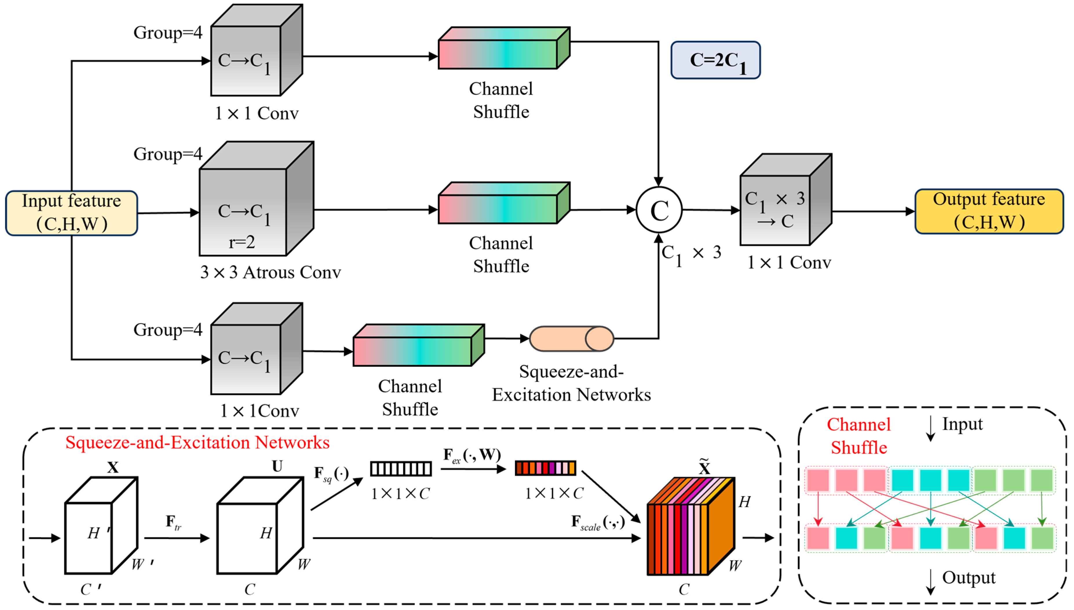
During the continuous convolution process of feature maps, some weakly salient information will be gradually weakened, blurred, and even disappear. However, these weakly featured targets may contain key information for the task targets, and the loss of this information can cause irreversible damage to the final detection. Therefore, this paper designs a feature enhancement module based on group shuffling, which aims to exchange more complete and reliable information for a minimal computational cost to improve the final detection accuracy. Its structure is shown in Figure 3. The enhancement module adopts a parallel topology with three branches. The first branch performs dimensionality reduction and expansion in the channel dimension through 1 × 1 grouped convolution, reducing model parameters. The calculation formulas are shown in Equations (1) and (2).
X 1 1 = σ π _ g g r o u p c o n v 1 1 X 0 ; W 1 1
X 1 = σ π _ g g r o u p c o n v 1 2 X 1 1 ; W 1 2
Here, X 0 represents the input feature map, and X 0 R C × H × W ; W i j denotes the convolution kernel weights of the i -th branch at the j -th stage, X 1 1 represents the feature map output after dimensionality reduction, g r o u p c o n v 1 1 and g r o u p c o n v 1 2 are the 1 × 1 convolutions responsible for channel compression and channel expansion, respectively. π _ g is in charge of dividing the input channels into g groups, with each sub-channel running convolutions only on its own channels. σ is the activation function, and X 1 is the feature output from the convolution of the first branch. During the dimensionality reduction process, channel grouping significantly reduces the computational load while ensuring detection accuracy.
The second branch employs 3 × 3 dilated grouped convolution, which can obtain the large receptive field corresponding to higher-parameter convolutions with fewer parameters, capturing local and global contextual information. The calculation process is consistent with the first branch, mainly expanding the receptive field through the dilation rate while still performing convolution within groups. The third branch combines 1 × 1 grouped convolution with attention enhancement, assigning weights to channel information. After convolution, the three branches are followed by a shuffle structure, which breaks the information barriers of grouped convolution and reconstructs cross-group dependencies at the cost of zero additional parameters. The SE attention calculation formulas are shown in Equations (3) and (4), and the output of this branch is shown in Equation (5).
z = 1 H × W h = 1 H w = 1 W X 3 1 h , w
α = σ W _ u p Re L U W _ d o w n z
X 3 = α X 3 1
The feature map X 3 1 from the third branch, after grouped convolution and channel shuffling, is compressed in the spatial dimension of H × W to obtain a global scalar z for each channel. It then sequentially passes through the channel compression weights and expansion weights W _ d o w n and W _ u p , ultimately obtaining a 0–1 weight vector α for each channel. The weight vector α is element-wise multiplied with X 3 1 to enhance important channels and suppress less important ones, resulting in the output X 3 of the third branch.
Finally, the outputs from the three branches are concatenated and followed by a 1 × 1 convolution to restore the number of channels, resulting in a feature map that integrates local detail information, global contextual information, and channel weights. This enhances the model’s ability to discern weak texture regions.

3.4. EGU

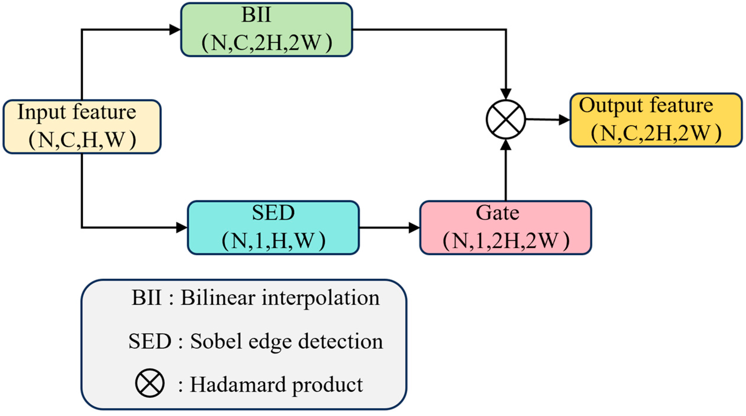
The background of maritime ships is characterized by uniform texture and color similarity to the ship’s hull. This can cause traditional upsampling methods to mistakenly identify weak edge high-frequency signals in the image as noise and smooth them out during the magnification process. This poses significant challenges for subsequent detection and localization. Therefore, this paper redesigns the upsampling process in the neck network. The Sobel operator is used to calculate edge confidence, and after magnification, a per-pixel weighting method is employed to better enhance the high-frequency structures of ships. The calculation process is shown in Equations (6)–(9).
G r a y = m e a n X , a x i s = C
G x = G r a y K x
G y = G r a y K y
M a g = G x 2 + G y 2 + ε
For the input tensor X , the reduction direction is specified as the channel dimension C , i.e., a x i c = C . Through global average pooling m e a n , a grayscale image G r a y is obtained. The grayscale image is then convolved with the horizontal and vertical Sobel kernels K x and K y , respectively, to obtain the horizontal gradient map G x for detecting vertical edges and the vertical gradient map G y for detecting horizontal edges. Finally, the two gradients are squared, added together, and the square root is taken to form the Euclidean norm, achieving efficient energy fusion. The output edge magnitude map M a g has larger values indicating more drastic changes. The constant ε in the equation is a numerical stability constant, set to 10−6 to avoid gradient explosion during backpropagation.
The newly designed upsampling module is named EGU, and its structure is shown in Figure 4. It can be seen that after the Sobel operator, a Gate control is connected, which assigns lower weights to aliasing areas, acting more like an adaptive filter. Pixels with higher gradients but lower proportions are given more weight. Therefore, the sea surface background information will be suppressed. The calculation formula for the gating mechanism is shown in Equation (10).
G a t e x , y = σ M a g x / 2 , y / 2 τ / T
Here, G a t e x , y represents the output gate map, M a g x / 2 , y / 2 denotes the edge magnitude map downsampled by a factor of two, is the integer coordinate mapping, i.e., nearest-neighbor sampling, τ is a fixed threshold hyperparameter, by randomly selecting 5000 images from the training set, obtaining histograms through Sobel filtering and normalization, extracting the valley quantiles, and conducting short-term ablation studies to determine the value of τ that corresponds to the highest AP value, which is 0.15. It serves as the baseline for determining significance, and T is the learnable temperature parameter, initially set to 1 and participating in backpropagation to achieve adaptive soft or hard gating. This mechanism suppresses background noise and enhances target features. The parallel bilinear interpolation upsamples the input feature map to obtain high-resolution features. In summary, the EGU module integrates edge display modeling, learnable amplification coefficients, and soft gate enhancement into a unified strategy, improving the neck network’s discriminative ability in scenarios with low sea surface contrast and slender ship structures without significantly increasing the inference burden.

3.5. R-IoU-Focal Loss Function

In the bounding box regression loss task of the YOLO model, the CIoU loss function is used by default, and this is also the case in the YOLOv8 model. The calculation formula for the CIoU loss function is shown in Equation (11).
L C I o U = 1 A B A B + ρ 2 A , B w c 2 + h c 2 + α ν α = ν 1 I o U + ν ν = 4 π 2 arctan w g t h g t arctan w p r e h p r e
The variables and parameters can be referred to in Figure 5. A represents the area of the ground-truth bounding box, B is the area of the predicted bounding box, ρ is the distance between the centers of the ground-truth and predicted boxes, h c and w c are the height and width of the smallest rectangle enclosing both the ground-truth and predicted boxes, h g t , w g t , h p r e , and w p r e are the heights and widths of the ground-truth and predicted boxes, α is the aspect ratio penalty weight coefficient, and ν is the measure of aspect ratio consistency.
Although the default CIoU loss function uses center point distance and shape ratio penalty, the challenges faced in this paper include the large aspect ratio of ships, imbalanced foreground and background distributions, and the similarity in color between ships and seawater, which results in similar low-level features that are not conducive to regression gradients. CIoU, by assigning the same weight to all samples, can lead to the issue of slender ship target bounding boxes having well-aligned centers but large differences in length. To address these issues, this paper designs a new type of loss function named R-IoU-Focal. The R-IoU-Focal loss function consists of three parts: LIoU, Ldis, and LFocal-IoU, as defined in Equation (12).
L R I o U F o c a l = L I o U + L d i s + L f o c a l I o U = 1 I o U + ρ 2 A , B w c 2 + h c 2 + ln 1 + ρ 2 w g t , w p r e 5 × ln 1 + w c 2 α 1 I o U 2 ln I o U
The key loss function in the formula is L F o c a l I o U , which, through reweighting, can amplify the contribution of positive samples with I o U > 0.5 and address the issue of gradient overshadowing. To maintain consistency with RetinaNet, α in Equation (12) is set to 0.75. In summary, the loss function proposed in this paper upgrades the traditional CIoU’s uniform regression to focused regression through two strategies: geometric penalty terms and Focal weights, significantly improving convergence speed and localization accuracy in the maritime ship detection task.

4. Experimental Results

4.1. DataSet

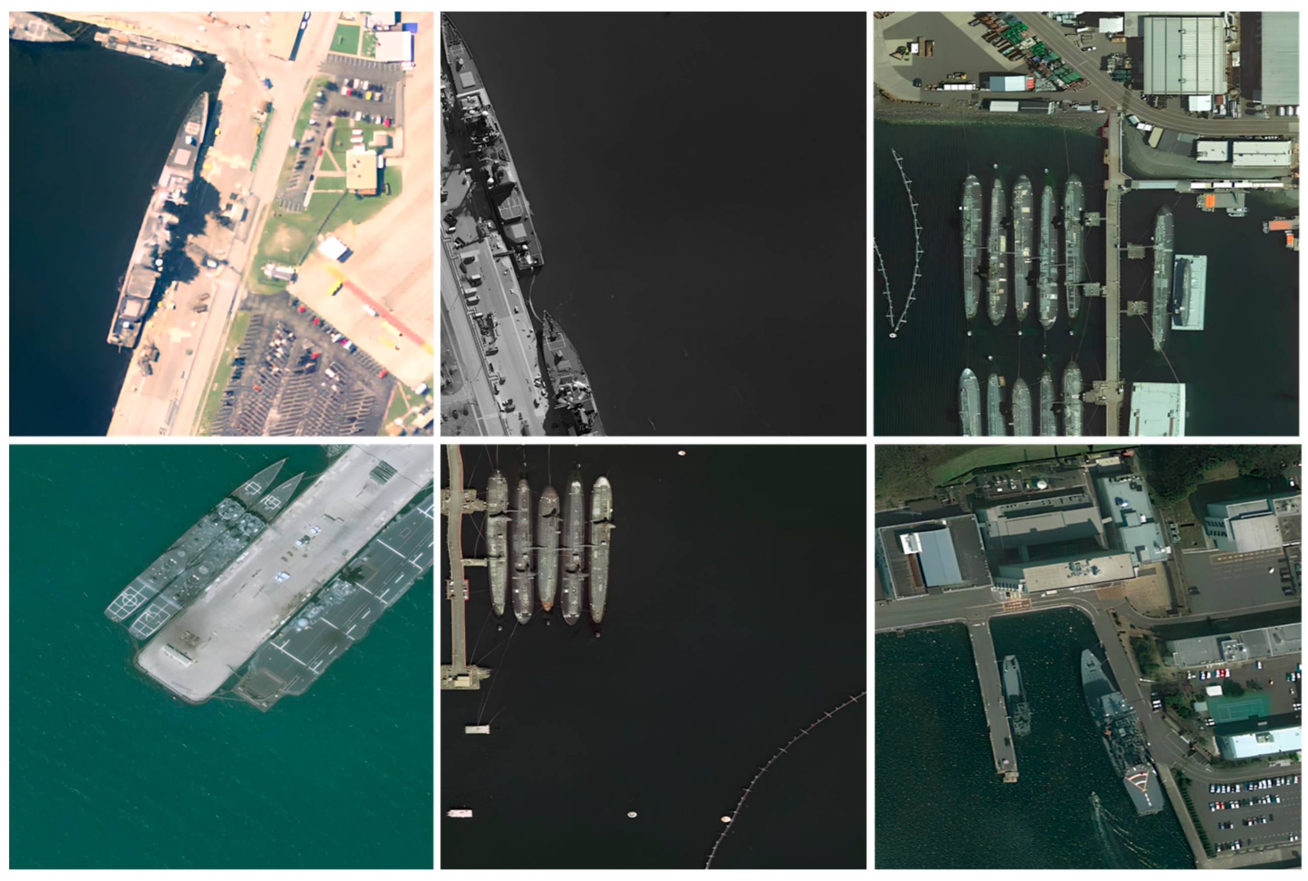
To more precisely validate the problems addressed by the proposed model, this paper employs a self-built dataset and an open-source dataset, naming the self-built dataset SlewSea-RS. In this dataset, there is only one target category, ships, without further classification of ships. However, SlewSea-RS boasts a large number of images, with the training set containing 14,000 images, the validation set containing 1700 images, and the test set containing 1700 images. The ratio of the training set, validation set, and test set conforms to the 8:1:1 proportion. The image sizes in each dataset range from 682 × 1024 to 1024 × 1024. As shown in Figure 6, which displays some sample scenes from the SlewSea-RS dataset, the ships in the images are slender targets, and the majority of the ships’ colors are similar to the background seawater. This paper extracts ship images from the open-source DOTA [41] dataset to construct a new dataset named DOTA-ship, which contains 1300 images, meeting the requirements for ship detection in this task.

4.2. Experimental Setup

The experiments in this paper were conducted on Ubuntu 18.04 operating system using PyTorch 1.9.1 and Python 3.8. The CPU and GPU used were Intel Core i7-9700k (Intel Corp., Santa Clara, CA, USA) and NVIDIA GeForce RTX 3090 Ti (NVIDIA Corp., Santa Clara, CA, USA), respectively. The GPU accelerator utilized was CUDA version 10.2. More detailed information about the experimental environment is listed in Table 1.
In addition, during the training phase, the stochastic gradient descent optimization algorithm was used to learn the parameters. The learning rate was uniformly set to 0.001, with a momentum of 0.937 and weight decay of 0.0005. The input image resolution was adjusted to 416 × 416, and the model was trained for 200 epochs with a batch size of 32, as shown in Table 2. To ensure the fairness of the experiments, all models used the same parameters during training and no image augmentation strategies were employed.

4.3. Evaluation Metric

To provide an objective evaluation of the model’s performance, this paper selects multiple evaluation metrics to analyze the model’s performance, including accuracy, recall, average precision, F1 score, as well as model parameters and computational complexity. The calculation formulas for accuracy and recall are shown in Equation (13).
P = T P T P + F P R = T P T P + F N
In the formula, T P represents true positives, F P represents false positives, and F N represents false negatives. An IoU threshold is set at 0.5, and then the precision and recall curves are plotted under this threshold condition. The curve drawn is known as the PR curve. The area under the curve, when integrated, forms a new evaluation metric called average precision, with the calculation formula shown in Equation (14). Since the dataset selected in this paper contains only one target category, ships, the average precision is numerically the same as the mean average precision in this case.
A P = 0 1 P R d R
From Equation (15), it can be seen that the metric F 1 balances precision and recall to evaluate the robustness of the model.
F 1 = 2 × P × R P + R

4.4. Results and Analysis

To more effectively validate the effectiveness of the proposed model, the following verification experiments were conducted in sequence, including comparison experiments with the baseline model, generalization experiments with more models, and ablation experiments to verify the effectiveness of each improved module.

4.4.1. Comparison Experiment

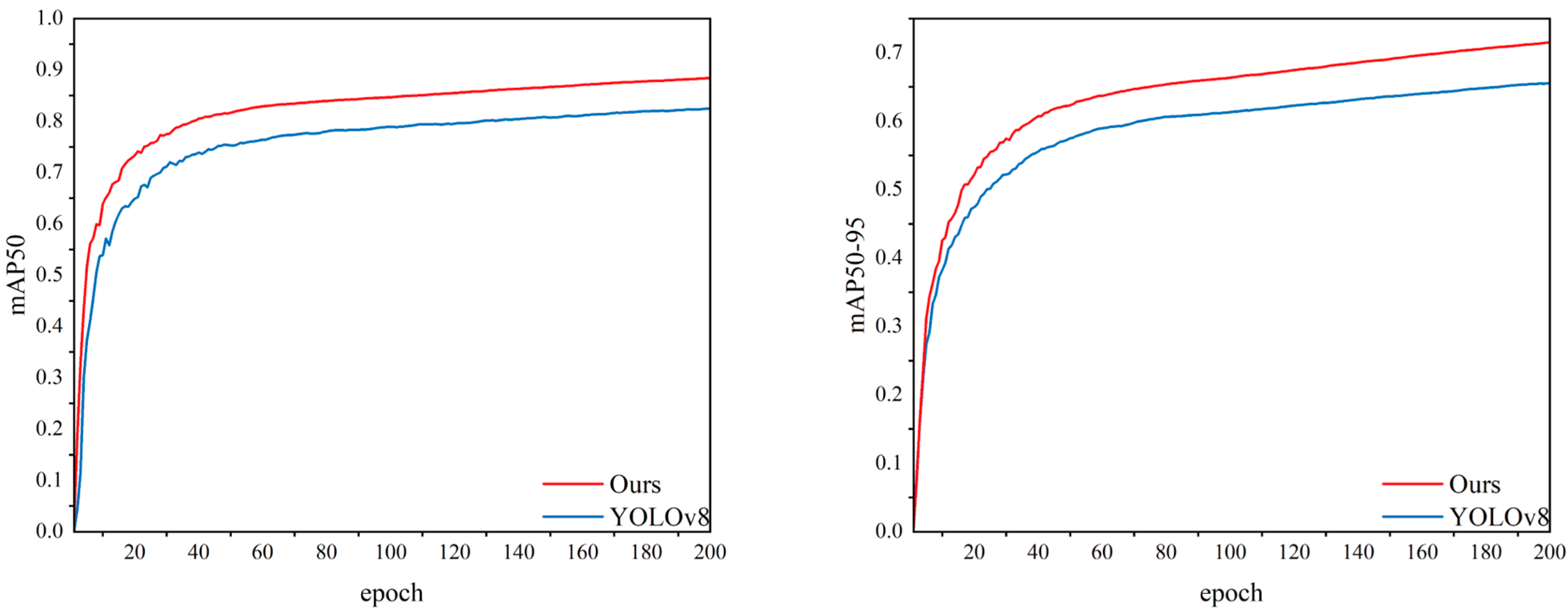
In this subsection, the performance improvement of the improved model relative to the original model is first verified. As shown in Figure 7, it depicts the performance evolution trend of the baseline model and the improved model during the training phase. The horizontal axis of both subplots represents the number of training epochs. The vertical axis of the left subplot indicates the mAP50 value, which has a relatively loose requirement, while the vertical axis of the right subplot indicates the mAP50–95 value, which has a stricter requirement. The two curves of different colors in the subplots represent the baseline model and the improved model, respectively, with annotations in the lower right corner of each subplot.
Analysis of the left image reveals that the detection performance of both curves rapidly increases and tends to saturate before 40 epochs. The performance of the improved model proposed in this paper consistently surpasses that of the baseline model. The right image exhibits the same trend. Even under stricter requirements, the improved model maintains its advantage. Therefore, the proposed model demonstrates superior performance in both detection recall and detection accuracy.
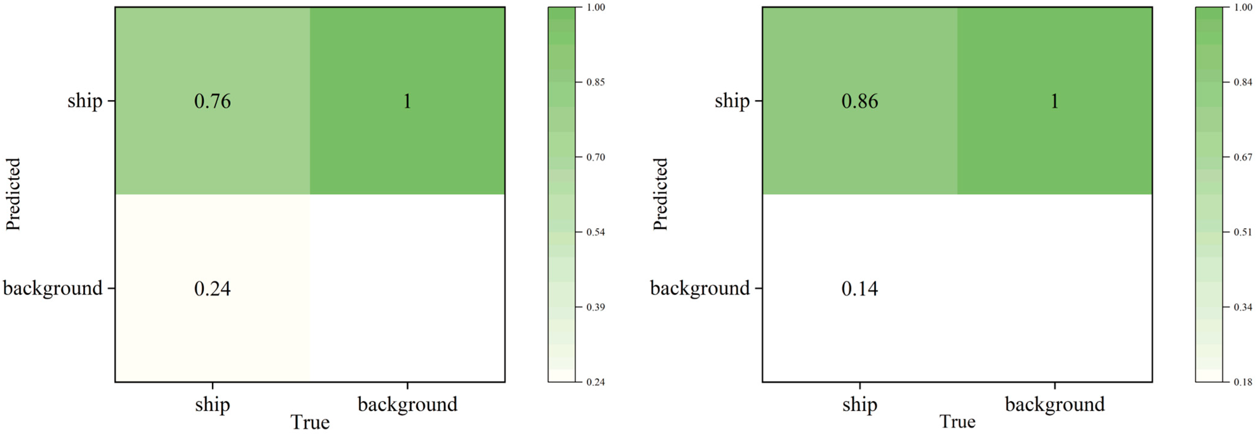
In addition, this paper also presents the normalized confusion matrices as shown in Figure 8. Both subplots in Figure 8 are based on the detection results of the SlewSea-RS dataset. The left subplot shows the detection results of the YOLOv8 model, while the right subplot shows the detection results of the proposed model. The horizontal axis of each subplot represents the actual target objects. Since the SlewSea-RS dataset contains only one category, ships, the actual target objects are divided into ships and background. The vertical axis represents the predicted target categories by the model. The data in the subplots indicate the model’s ability to distinguish between foreground and background, as well as the distribution of missed detections and false alarms.
Analysis of the two subplots in Figure 8 reveals that the proportion of actual ships correctly detected by the proposed model has increased by 10 percentage points compared to the original model, significantly reducing the miss rate. The improved model demonstrates better robustness for small, blurry, and occluded ships. Additionally, the improved model has a lower probability of misclassifying actual ships as background. Therefore, the proposed model achieves better recall in the ship detection task, and the proposed strategies enhance the model’s ability to distinguish between foreground and background.
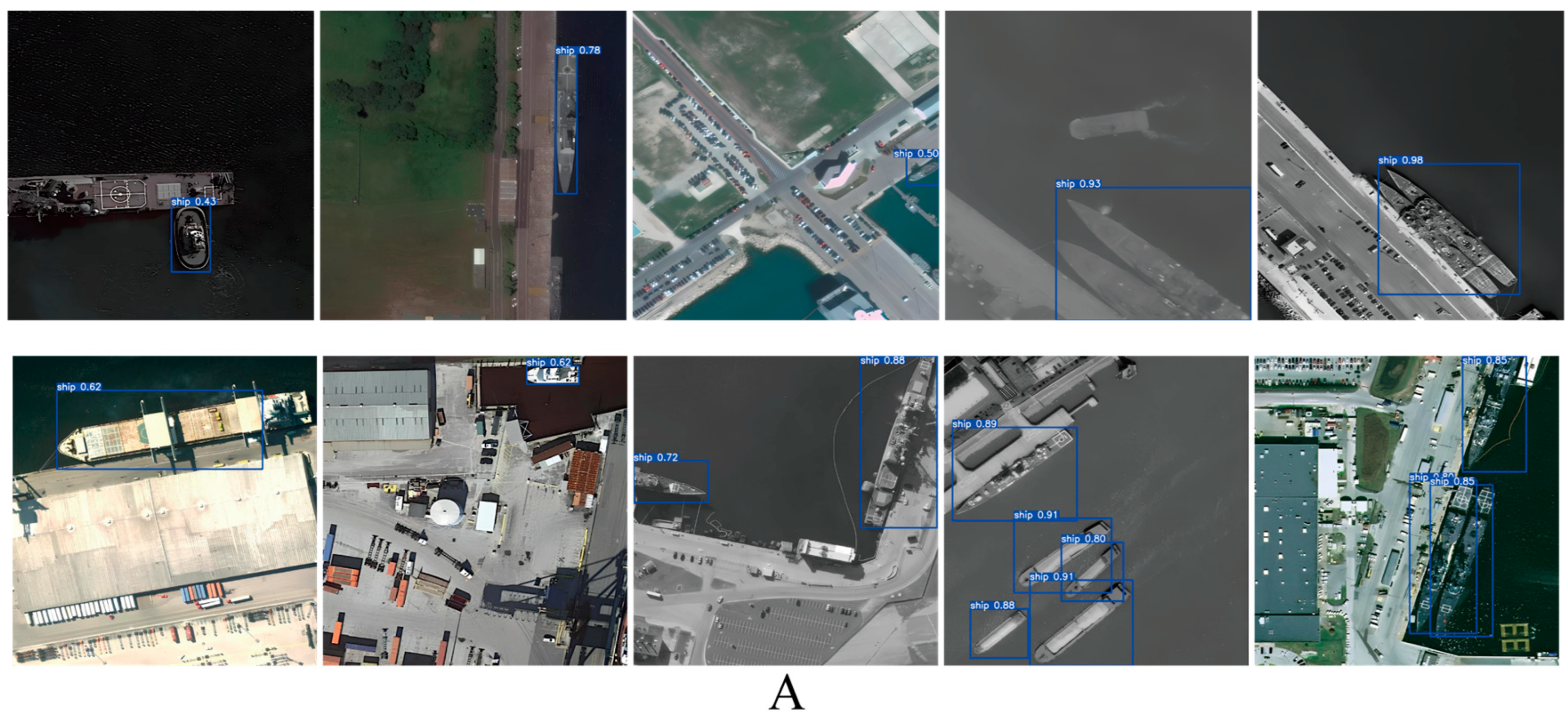
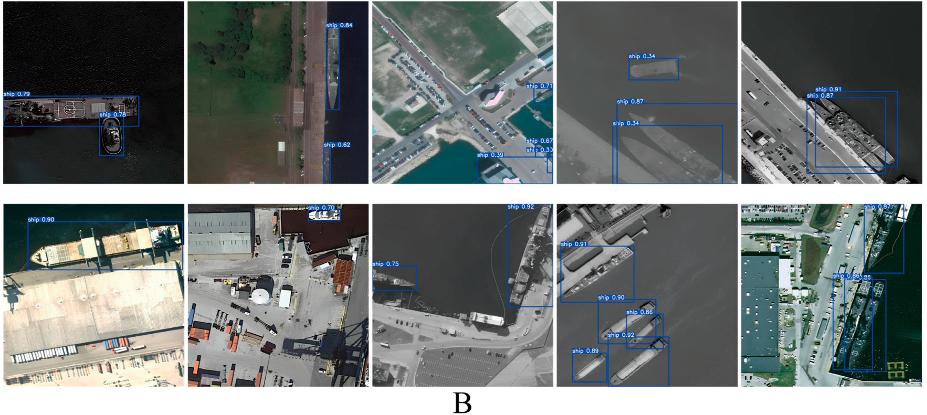
Finally, more intuitive visualization is used to compare the detection performance of the two models. As shown in Figure 9, it displays the detection results of the two models under different scenarios. Part A shows the detection results of the baseline model YOLOv8, while Part B shows the detection results of the improved model CSBI-YOLO.
Comparison of the results in Parts A and B reveals that in the first row scenario, the YOLOv8 model has missed detections, and in the fifth column of the first row, it merged two ships into one. The proposed model, however, demonstrates a lower miss rate and successfully detects the two closely adjacent ships separately. In the scenario of the first image in the second row, due to the extremely imbalanced length-to-width ratio of the ship, the original model’s predicted bounding box failed to fully cover the ship. The improved model, however, effectively addresses this issue. Additionally, in other scenarios, the improved model shows better detection accuracy, confirming that compared to the baseline model, the proposed model has superior performance.

4.4.2. Generalization Experiment

To conduct more extensive experiments, this subsection performs experiments and comparative analyses on multiple models using both the self-built SlewSea-RS dataset and the DOTA-ship dataset created based on the open-source DOTA [41] dataset.
Table 3 and Table 4 present the performance comparison of seven models based on the SlewSea-RS dataset and the DOTA-ship dataset, respectively. The selected models for comparison include three two-stage detection models, namely Fast R-CNN [42], Faster R-CNN [12], and Cascade R-CNN [43], as well as three one-stage detection models that are widely used in research applications, namely YOLOv5, YOLOv8 [20], and YOLOv11 [23]. The performance metrics used for comparison are model parameters, computational complexity, Precision, Recall, mAP50, and mAP50–95.
Analysis of the data in Table 3 and Table 4 reveals that the two-stage detection models have significantly higher model parameters and computational complexity compared to one-stage detection models, and their detection accuracy also lags behind the advanced YOLO series models. In the comparison results on the SlewSea-RS dataset, CSBI-YOLO leads in detection accuracy. Compared to YOLOv8, the detection precision of CSBI-YOLO increased by 5.4%, and compared to YOLOv11, it increased by 3.2%. The mAP50 of CSBI-YOLO increased by 6% compared to YOLOv8 and by 2.6% compared to YOLOv11. On the DOTA-ship dataset, the detection precision of CSBI-YOLO even exceeded 90%. Compared to YOLOv8 and YOLOv11, the mAP50 of CSBI-YOLO increased by 1.3% and 1%, respectively, and the mAP50–95 increased by 1% and 1.8%, respectively. This indicates that in comparisons with more models, the proposed model still demonstrates superior detection performance. Although there is a slight increase in parameters and computational complexity, this minor increase in computation is necessary to achieve a greater improvement in detection quality.
In addition, a bidirectional grouped bar chart of the F1 score, as shown in Figure 10, was drawn. The horizontal axis of the chart represents the bidirectional changes in the F1 score, while the vertical axis represents the seven compared models. The blue side of the chart indicates the results based on the SlewSea-RS dataset, and the red side indicates the results based on the DOTA-ship dataset. The data on both sides of the bar chart represent the F1 score values of the corresponding models.
Analysis of the data in Figure 10 reveals that, despite the small differences in F1 scores among different models across the two datasets, the CSBI-YOLO model still achieves the highest F1 score. As seen in Table 4, the detection precision of Fast R-CNN is 1.4% lower than that of YOLOv5. However, on the red side representing the DOTA-ship dataset, Fast R-CNN’s F1 score is 0.3% higher than that of YOLOv5. This illustrates that the F1 score is a comprehensive metric. The higher F1 score of the proposed model indicates a better balance between precision and recall, resulting in more reliable detection outcomes.
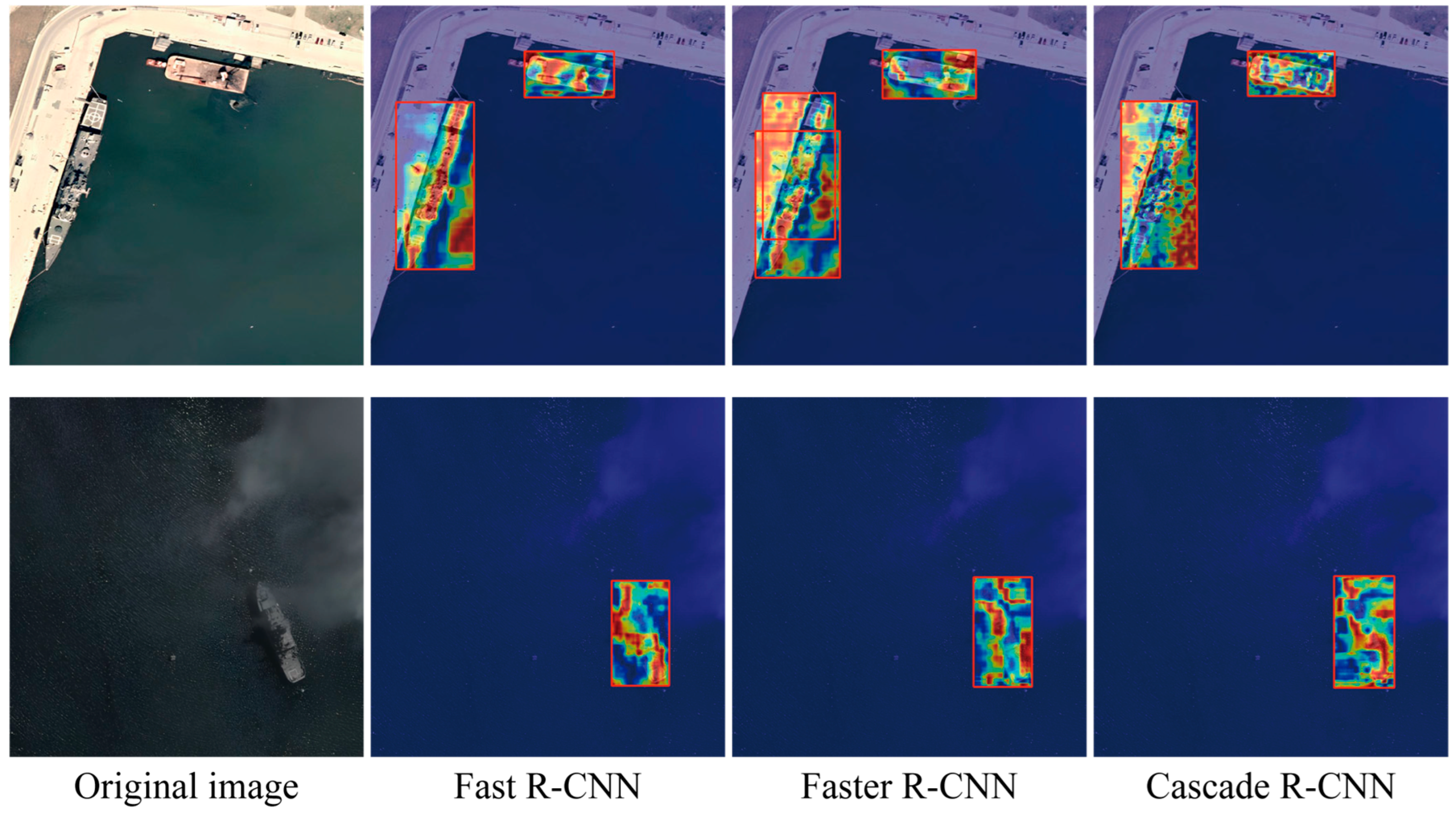
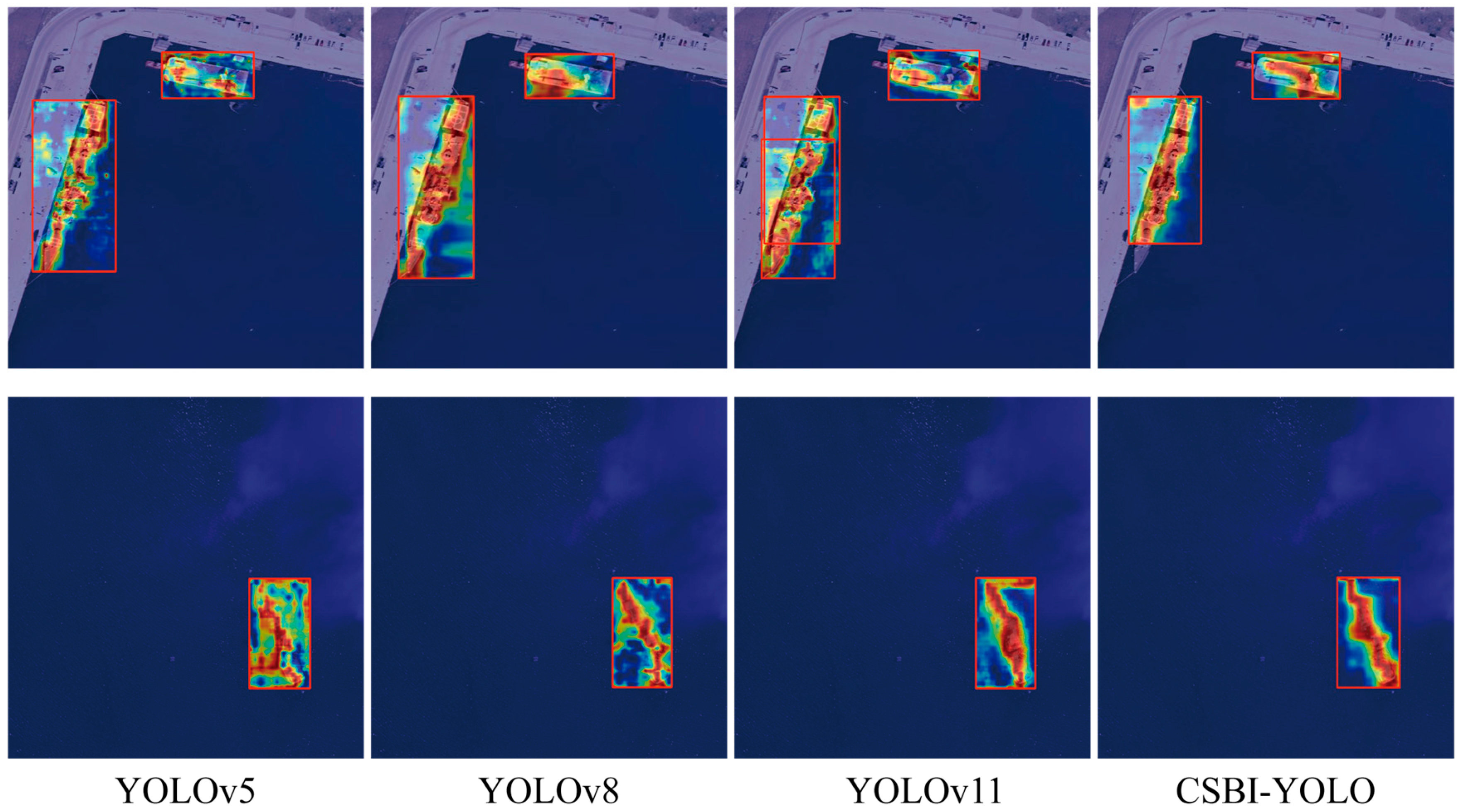
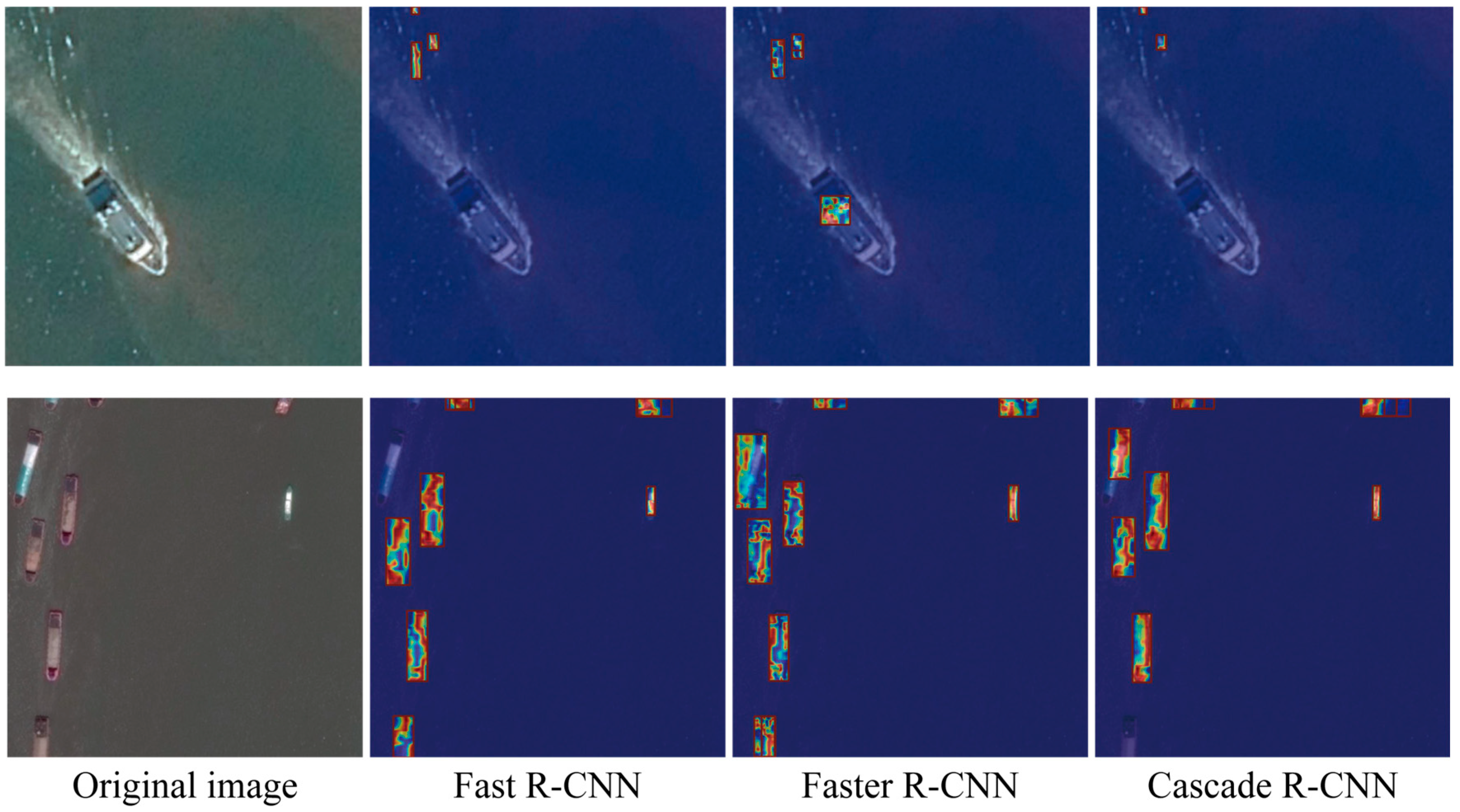
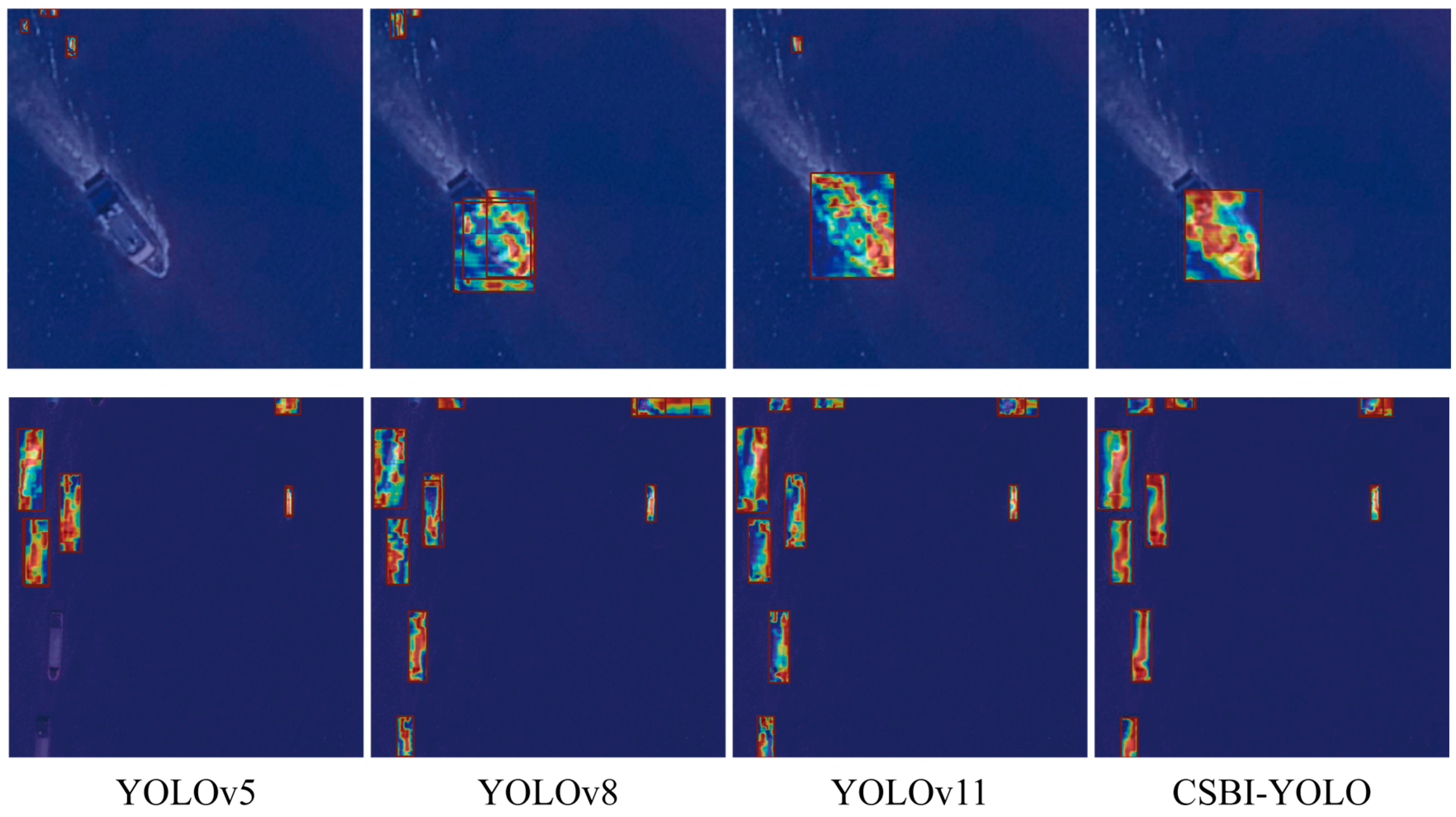
To more intuitively compare the detection effects of the models, visualization heatmaps as shown in Figure 11 and Figure 12 are presented. Figure 11 displays the detection results based on the SlewSea-RS dataset, while Figure 12 shows the results based on the DOTA-ship dataset. In Figure 11, it can be observed that the detection results of other models have varying degrees of background response, with high brightness appearing in the background areas. In contrast, the detection results of the CSBI-YOLO model show high brightness tightly surrounding the ground-truth boxes, indicating accurate localization. In the results shown in Figure 12, all other models misidentified the waves as ships, while only a few models were able to detect the actual ships. The proposed model, however, not only avoided misidentification but also accurately localized the ships, demonstrating its effectiveness on the DOTA-ship dataset.

4.4.3. Ablation Experiment

To analyze the effectiveness of each improvement strategy in the CSBI-YOLO model, GS-FEM, EGU, and the R-IoU-Focal loss function were successively added to the baseline model to verify their effectiveness.
As shown in Table 5, ablation experiments were conducted on the SlewSea-RS dataset. Single strategies and combinations of two strategies were successively introduced into the YOLOv8 model, resulting in a comparison of eight models. As can be seen from the data presented in Table 5, the increase in model parameters is mainly due to the feature enhancement module GS-FEM, while the increase in parameters caused by EGU is minimal. In terms of computational complexity, the addition of the GS-FEM module is the most significant, but it also brings a relatively noticeable improvement in detection accuracy. Looking at the effects of individual strategies, the R-IoU-Focal loss function has the largest increase. When combining two strategies, the combination of the feature enhancement module and the loss function performs the best, and it is higher than the sum of the independent gains of the two methods. Overall, the introduction of all strategies has improved the model’s performance to varying degrees. Although the detection speed has slightly decreased, it still meets the requirements for real-time detection.
To more meticulously validate the rationality and effectiveness of the tri-branch design of the GS-FEM module, taking GS-FEM as the baseline model, the three branches were added in sequence from top to bottom, named Branch one, Branch two, and Branch three, respectively. Additionally, a Branch four was added at the bottom, composed of a 3 × 3 dilated grouped convolution. On the basis of incrementally adding each branch, the positions of the grouped convolution and channel shuffling were swapped to verify the optimal placement of the channel shuffling mechanism. The results of the ablation experiments are shown in Table 6.
The design of Table 6 is based on the GS-FEM module, which is why there are no specific metrics for GS-FEM in terms of parameters and mAP50. The subsequent performance changes due to the use of individual branches and the relocation of the shuffling mechanism are also based on the GS-FEM module. This explains the occurrence of data showing an 85% reduction in parameters and a 72% drop in mAP50. An analysis of the changes in parameters and mAP50 reveals that as the number of branches increases, both parameters and mAP50 rise in tandem. For the same branch with different shuffling positions, employing channel shuffling first results in a negligible reduction in parameters but a severe impact on detection accuracy. Moreover, when the number of branches reaches four, there is a significant increase in parameters, yet a substantial decline in performance. It can be concluded that the design of three branches and the positioning of channel shuffling have achieved optimal conditions, thereby validating the rationality of the GS-FEM module design.
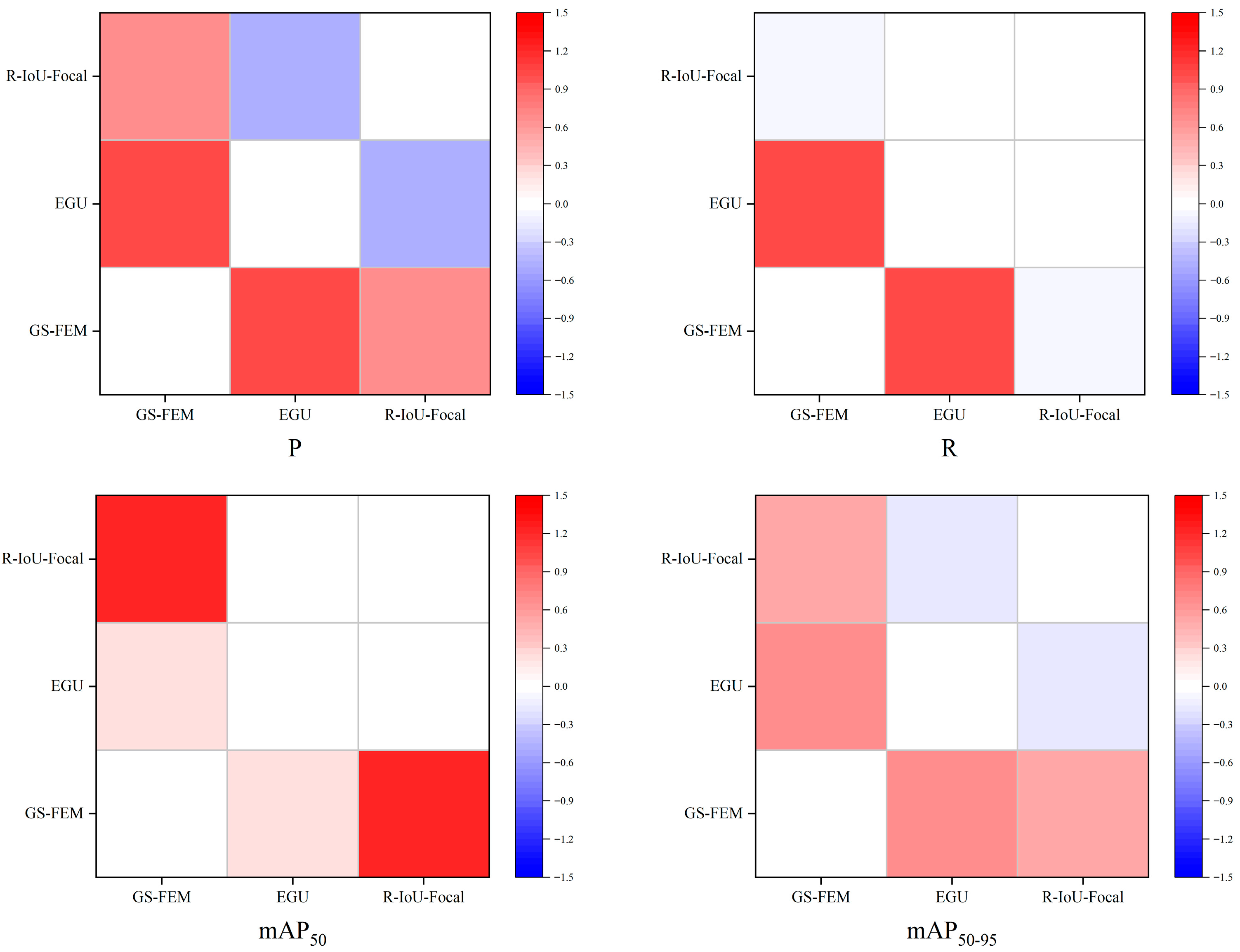
In addition, to more comprehensively analyze the interrelationships among the three strategies, a collaborative benefit heatmap as shown in Figure 13 was drawn. The definition of synergistic effect is as follows:
C x , y = M A + B x , y M b a s e l i n g x , y M A x , y M b a s e l i n g x , y M B x , y M b a s e l i n g x , y
In the formula, M A + B x , y represents the model performance when both A and B are used simultaneously, M b a s e l i n g x , y represents the performance of the baseline model, and M A x , y and M B x , y represent the model performance when modules A and B are used individually.
Simply put, it determines whether the combined use of any two strategies is better than or worse than the sum of their individual effects. This paper uses a heatmap to intuitively display the results. As can be seen in Figure 13, there are four subplots, each representing the collaborative benefit analysis under four performance metrics: precision, recall, mAP50, and mAP50–95. The deeper the red, the better the collaborative boost of the two strategies; the deeper the blue, the higher the collaborative negative effect of the combined use of the two strategies; white indicates that the combined effect of the two strategies is equivalent to the sum of their individual effects. Since the negative diagonal positions in each subplot represent the same strategy, these positions are displayed in white.
Analysis of the four subplots in Figure 13 reveals that in the heatmap for precision, the combination of EGU and the R-IoU-Focal loss function exhibits a negative collaborative effect. The combination of GS-FEM and EGU shows a positive collaborative boost, achieving better performance. There is also some negative synergy in the recall and mAP50–95 metrics, but no negative synergy exists in the mAP50 metric.
From these four sub-heatmaps, it can be seen that while some combinations of strategies are not ideal, the majority of combined methods still show good collaborative effects in enhancing performance.
We analyzed the principles of EGU and the loss function and found that the EGU module suppresses low-response areas through a gating mechanism, while the loss function amplifies the weights of low-IoU parts. This leads to the network forcibly fitting the weak features suppressed by the EGU module, resulting in a contradiction and ultimately manifesting as a negative synergistic effect.
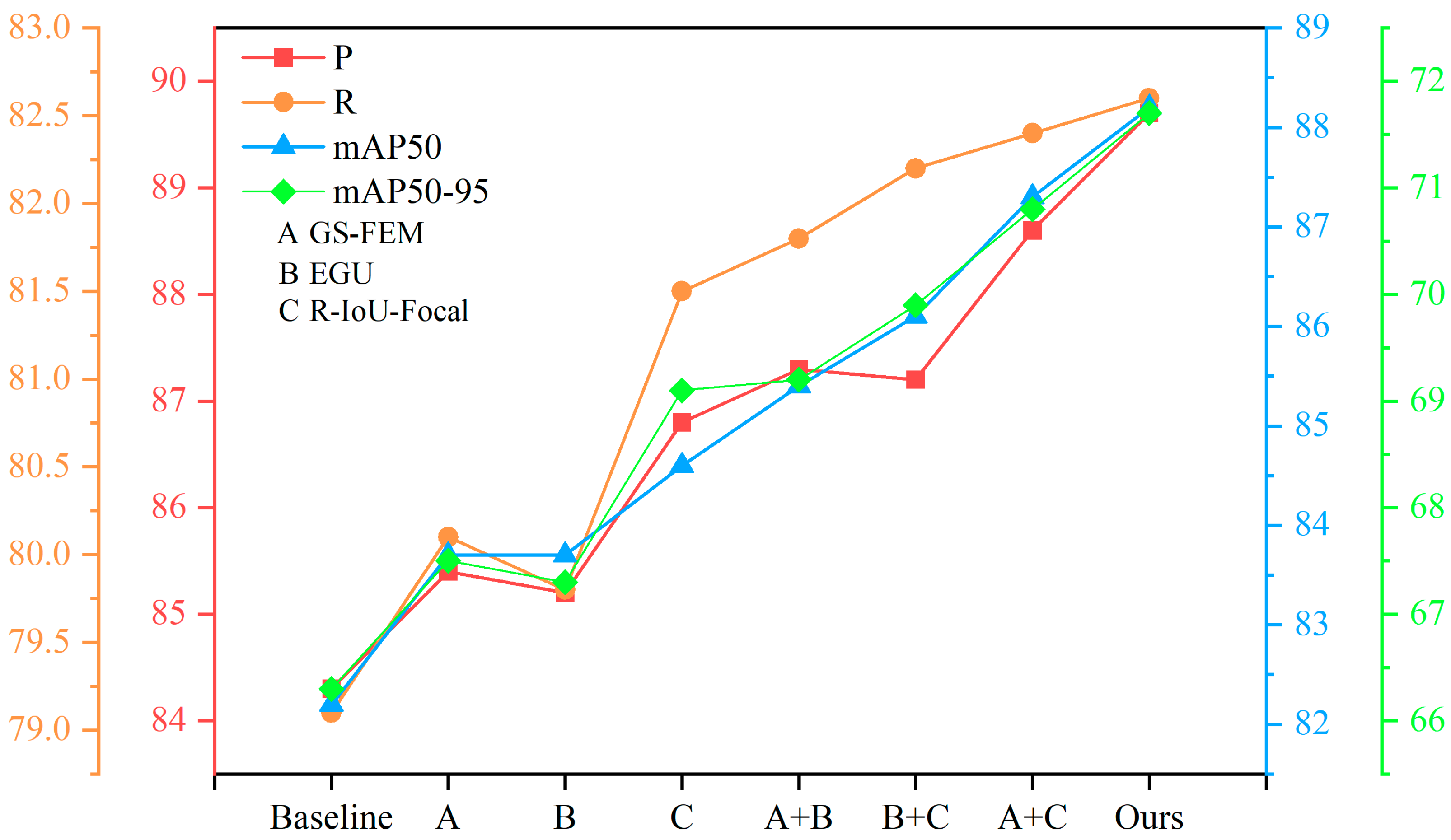
Figure 14 is a four-axis line chart drawn based on the changes in model performance after the introduction of different methods. It provides a more intuitive view of how performance evolves with the gradual addition of modules. The horizontal axis in Figure 14 represents models using different modules, while the vertical axis uses four differently colored Y-axes to indicate changes in four different performance metrics, corresponding to the colors of the lines in the chart. The performance metrics represented by different colors are labeled in the upper left corner of the figure.
Analysis of the trend in the lines in Figure 14 reveals that the GS-FEM module generally contributes more to model performance improvement than the EGU module, and the R-IoU-Focal loss function has the best effect, which is consistent with the data in Table 5.
Finally, visualization heatmaps are provided for models with the GS-FEM module and the R-IoU-Focal loss function introduced separately, as shown in Figure 15. After the GS-FEM module is introduced alone, compared with the baseline model, the highlighted areas are more concentrated, with fewer highlights appearing in the background areas. This demonstrates the effectiveness of the GS-FEM module in enhancing ship features and suppressing background information. Observing the heatmap with the R-IoU-Focal loss function introduced, it can be seen that its detection box fully encompasses the targets in the scene, while the baseline model does not cover all the targets in the scene. This proves the advantage of the R-IoU-Focal loss function in considering the length-to-width ratio of ships.

5. Discussion

Visible light remote sensing images have higher resolutions and can provide richer detail information, with a wide range of applications. However, traditional detection methods perform poorly when dealing with challenges such as ships having colors similar to the background waves and extreme length-to-width ratios of ships. More detailed information differentiation of ship targets and further optimization of extreme ship proportions are expected to address these two major challenges, thereby improving the efficiency and quality of various ship detection tasks. The most significant finding of this paper is that by combining grouped channel shuffling, edge gating, and the R-IoU-Focal loss function, the mAP50 and mAP50–95 were increased by 6% and 5.4%, respectively, in scenarios with extreme ship length-to-width ratios and overlapping sea colors. The reliability was also verified on two datasets. However, some issues were identified during the research process. First, there was insufficient parameter increase. The channel shuffling feature enhancement module used increases the overall network parameters. Although it still meets the real-time detection requirements, considering the current trend towards more lightweight models in extensive research, the grouped convolution in the module structure is most likely to contribute the most to the parameter increase, but this has not been experimentally verified. Further research on this issue in the next step can be more in-depth by comparing different convolution types to observe changes in parameters and detection accuracy, seeking strategies that can both improve detection performance and achieve lightweighting. The second issue is the negative synergy found in the collaborative thermal efficiency experiment between the EGU module used and the improved loss function. Only theoretical possible reasons were analyzed in the paper. Such negative synergy is undesirable, indicating conflicts between these two strategies. Therefore, further investigation into the causes of this conflict and experimental exploration for solutions are needed in the next step of work to enhance the rationality of the network structure and the overall performance of the model.

6. Conclusions

All research and experiments in this paper are centered on addressing the issues of imbalanced length-to-width ratios of ships and sea surface background interference in maritime ship detection tasks. To this end, three improvement strategies have been designed. First, considering that the sea water, which is similar in color to ships, can interfere with ship feature extraction, a feature enhancement module named GS-FEM is designed. It employs grouped convolution and channel shuffling mechanisms to process input information in parallel. Channel shuffling breaks the information barriers of grouped convolution, combining semantic information across different scales to extract more effective features. Second, a new upsampling unit named the EGU module is constructed, featuring parallel bilinear interpolation and an adaptive gating mechanism. The Sobel magnitude operator is used to suppress sea surface noise. Finally, a loss function named R-IoU-Focal is designed to address the imbalanced length-to-width ratios of ship targets. This loss function not only considers the position and shape of the targets but also their scale, resolving the performance deficiencies of previous models in detecting ship targets. Extensive experiments were conducted on the self-built SlewSea-RS dataset. Compared to the baseline model, the mAP50 value increased from 82.2% to 88.2%, and the mAP50–95 value rose from 66.3% to 71.7%. Experiments were also performed on the DOTA-ship dataset, which is based on the open-source remote sensing dataset DOTA and focuses solely on ships. Compared to the baseline model, the mAP50 value improved by 1.3%, and the mAP50–95 value increased by 1%. In comparative experiments with other models on these two datasets, the proposed CSBI-YOLO model demonstrated superior performance, confirming its excellent capabilities in maritime ship detection tasks.
Although CSBI-YOLO leads in various detection accuracy metrics, it still introduces a slight increase in parameters and complexity compared to the baseline model. The increase in parameters is mainly due to the GS-FEM module. Moreover, the negative synergy between different strategies cannot be ignored. Our future work will focus on the lightweighting of the feature enhancement module and the optimization of collaborative gains between different strategies.

Author Contributions

S.L. and J.X.; methodology, F.S.; software, J.D.; validation, W.C. and S.L.; resources, F.S.; data curation, F.S.; writing—original draft preparation, S.L.; writing—review and editing, S.L.; visualization, S.L.; supervision, Q.L.; project administration, T.Z.; funding acquisition, F.S. All authors have read and agreed to the published version of the manuscript.

Funding

This research was funded by the National Natural Science Foundation of China (grant. number: 61671470).

Data Availability Statement

Data is contained within the article. The original contributions presented in this study are included in the article. Further inquiries can be directed to the corresponding author.

Conflicts of Interest

The authors declare no conflicts of interest.

References

  1. Zhang, H.; Chen, M. A Decade of Monitoring On-Road Vehicle Emissions Using Remote Sensing Technology. Int. J. Hydrog. Energy 2025, 130, 605–614. [Google Scholar] [CrossRef]
  2. Liu, Y. Application of Remote Sensing Technology in Smart City Construction and Planning. J. Phys. Conf. Ser. 2023, 2608, 012052. [Google Scholar] [CrossRef]
  3. Sun, Y.; Wang, D.; Li, L.; Ning, R.; Yu, S.; Gao, N. Application of Remote Sensing Technology in Water Quality Monitoring: From Traditional Approaches to Artificial Intelligence. Water Res. 2024, 267, 122546. [Google Scholar] [CrossRef]
  4. Mohsan, S.A.H.; Khan, M.A.; Ghadi, Y.Y. Editorial on the Advances, Innovations and Applications of UAV Technology for Remote Sensing. Remote Sens. 2023, 15, 5087. [Google Scholar] [CrossRef]
  5. Casagli, N.; Intrieri, E.; Tofani, V.; Gigli, G.; Raspini, F. Landslide Detection, Monitoring and Prediction with Remote-Sensing Techniques. Nat. Rev. Earth Environ. 2023, 4, 51–64. [Google Scholar] [CrossRef]
  6. Battison, R.; Prober, S.M.; Zdunic, K.; Jackson, T.D.; Fischer, F.J.; Jucker, T. Tracking Tree Demography and Forest Dynamics at Scale Using Remote Sensing. New Phytol. 2024, 244, 2251–2266. [Google Scholar] [CrossRef] [PubMed]
  7. Wang, G.; Li, H.; Xiao, Q.; Yu, P.; Ding, Z.; Wang, Z.; Xie, S. Fighting against Forest Fire: A Lightweight Real-Time Detection Approach for Forest Fire Based on Synthetic Images. Expert Syst. Appl. 2025, 262, 125620. [Google Scholar] [CrossRef]
  8. Yar, H.; Ullah, F.U.M.; Khan, Z.A.; Kim, M.J.; Baik, S.W. EFNet-CSM: EfficientNet with a Modified Attention Mechanism for Effective Fire Detection. Knowl.-Based Syst. 2025, 329, 114353. [Google Scholar] [CrossRef]
  9. Liu, Q.; Chen, S.; Liu, G.; Yang, L.; Yuan, Q.; Cai, Y.; Chen, L. Dual-Perspective Safety Driver Secondary Task Detection Method Based on Swin-Transformer and Cross-Attention. Adv. Eng. Inform. 2025, 65, 103320. [Google Scholar] [CrossRef]
  10. Chen, Z.; Chen, H.; Imani, M.; Chen, R.; Imani, F. Vision Language Model for Interpretable and Fine-Grained Detection of Safety Compliance in Diverse Workplaces. Expert Syst. Appl. 2025, 265, 125769. [Google Scholar] [CrossRef]
  11. Girshick, R.; Donahue, J.; Darrell, T.; Malik, J. Region-Based Convolutional Networks for Accurate Object Detection and Segmentation. IEEE Trans. Pattern Anal. Mach. Intell. 2016, 38, 142–158. [Google Scholar] [CrossRef]
  12. Ren, S.; He, K.; Girshick, R.; Sun, J. Faster R-CNN: Towards Real-Time Object Detection with Region Proposal Networks. IEEE Trans. Pattern Anal. Mach. Intell. 2017, 39, 1137–1149. [Google Scholar] [CrossRef]
  13. He, K.; Gkioxari, G.; Dollar, P.; Girshick, R. Mask R-CNN. IEEE Trans. Pattern Anal. Mach. Intell. 2020, 42, 386–397. [Google Scholar] [CrossRef]
  14. Redmon, J.; Divvala, S.; Girshick, R.; Farhadi, A. You Only Look Once: Unified, Real-Time Object Detection. In Proceedings of the 2016 IEEE Conference on Computer Vision and Pattern Recognition (CVPR), Las Vegas, NV, USA, 27–30 June 2016; IEEE: Piscataway, NJ, USA, 2016; pp. 779–788. [Google Scholar]
  15. Redmon, J.; Farhadi, A. YOLO9000: Better, Faster, Stronger. In Proceedings of the 2017 IEEE Conference on Computer Vision and Pattern Recognition (CVPR), Honolulu, HI, USA, 21–26 July 2017; IEEE: Piscataway, NJ, USA, 2017; pp. 6517–6525. [Google Scholar]
  16. Redmon, J.; Farhadi, A. YOLOv3: An Incremental Improvement 2018. arXiv 2018, arXiv:1804.02767. [Google Scholar]
  17. Bochkovskiy, A.; Wang, C.-Y.; Liao, H.-Y.M. YOLOv4: Optimal Speed and Accuracy of Object Detection 2020. arXiv 2020, arXiv:2004.10934. [Google Scholar]
  18. Li, C.; Li, L.; Jiang, H.; Weng, K.; Geng, Y.; Li, L.; Ke, Z.; Li, Q.; Cheng, M.; Nie, W.; et al. YOLOv6: A Single-Stage Object Detection Framework for Industrial Applications 2022. arXiv 2022, arXiv:2209.02976. [Google Scholar]
  19. Wang, C.-Y.; Bochkovskiy, A.; Liao, H.-Y.M. YOLOv7: Trainable Bag-of-Freebies Sets New State-of-the-Art for Real-Time Object Detectors. In Proceedings of the 2023 IEEE/CVF Conference on Computer Vision and Pattern Recognition (CVPR), Vancouver, BC, Canada, 17–24 June 2023; IEEE: Piscataway, NJ, USA, 2023; pp. 7464–7475. [Google Scholar]
  20. Liu, S.; Shao, F.; Chu, W.; Dai, J.; Zhang, H. An Improved YOLOv8-Based Lightweight Attention Mechanism for Cross-Scale Feature Fusion. Remote Sens. 2025, 17, 1044. [Google Scholar] [CrossRef]
  21. Yi, W.; Xia, S.; Kuzmin, S.; Gerasimov, I.; Cheng, X. RTFVE-YOLOv9: Real-Time Fruit Volume Estimation Model Integrating YOLOv9 and Binocular Stereo Vision. Comput. Electron. Agric. 2025, 236, 110401. [Google Scholar] [CrossRef]
  22. Pan, W.; Chen, J.; Lv, B.; Peng, L. Lightweight Marine Biodetection Model Based on Improved YOLOv10. Alex. Eng. J. 2025, 119, 379–390. [Google Scholar] [CrossRef]
  23. Liu, S.; Shao, F.; Yang, C.; Dai, J.; Xue, J.; Liu, Q.; Zhang, T. ACLC-Detection: A Network for Remote Sensing Image Detection Based on Attention Mechanism and Lightweight Convolution. Remote Sens. 2025, 17, 2572. [Google Scholar] [CrossRef]
  24. Hu, H.; Chen, S.; You, Z.; Tang, J. FSENet: Feature Suppression and Enhancement Network for Tiny Object Detection. Pattern Recognit. 2025, 162, 111425. [Google Scholar] [CrossRef]
  25. Xie, G.; Wu, X.; Shi, J.; Su, Y.; Shi, B. Enhancing Real-Time Detection Transformer for Small Floating Targets. Eng. Appl. Artif. Intell. 2025, 161, 112038. [Google Scholar] [CrossRef]
  26. Tang, Y.; Luo, F.; Wu, P.; Tan, J.; Wang, L.; Niu, Q.; Li, H.; Wang, P. An Improved YOLO Network for Small Target Insects Detection in Tomato Fields. Comput. Electron. Agric. 2025, 239, 110915. [Google Scholar] [CrossRef]
  27. Chen, Y.; Wang, T.; Chen, G.; Zhu, K.; Tan, X.; Wang, J.; Guo, W.; Wang, Q.; Luo, X.; Zhang, X. BFA-YOLO: A Balanced Multiscale Object Detection Network for Building Façade Elements Detection. Adv. Eng. Inform. 2025, 65, 103289. [Google Scholar] [CrossRef]
  28. Zhou, S.; Zhang, M.; Wu, L.; Yu, D.; Li, J.; Fan, F.; Zhang, L.; Liu, Y. Lightweight SAR Ship Detection Network Based on Transformer and Feature Enhancement. IEEE J. Sel. Top. Appl. Earth Obs. Remote Sens. 2024, 17, 4845–4858. [Google Scholar] [CrossRef]
  29. He, H.; Hu, T.; Xu, S.; Xu, H.; Song, L.; Sun, Z. PPDM-YOLO: A Lightweight Algorithm for SAR Ship Image Target Detection in Complex Environments. IEEE J. Sel. Top. Appl. Earth Obs. Remote Sens. 2025, 18, 22690–22705. [Google Scholar] [CrossRef]
  30. Zhu, M.; Han, D.; Han, B.; Huang, X. YOLO-HPSD: A High-Precision Ship Target Detection Model Based on YOLOv10. PLoS ONE 2025, 20, e0321863. [Google Scholar] [CrossRef]
  31. Tan, X.; Leng, X.; Luo, R.; Sun, Z.; Ji, K.; Kuang, G. YOLO-RC: SAR Ship Detection Guided by Characteristics of Range-Compressed Domain. IEEE J. Sel. Top. Appl. Earth Obs. Remote Sens. 2024, 17, 18834–18851. [Google Scholar] [CrossRef]
  32. Feng, Y.; Zhang, Y.; Zhang, X.; Wang, Y.; Mei, S. Large Convolution Kernel Network With Edge Self-Attention for Oriented SAR Ship Detection. IEEE J. Sel. Top. Appl. Earth Obs. Remote Sens. 2025, 18, 2867–2879. [Google Scholar] [CrossRef]
  33. Li, S.; Yan, F.; Liu, Y.; Shen, Y.; Liu, L.; Wang, K. A Multi-Scale Rotated Ship Targets Detection Network for Remote Sensing Images in Complex Scenarios. Sci. Rep. 2025, 15, 2510. [Google Scholar] [CrossRef] [PubMed]
  34. Fu, Y.; Fang, W. Incorporating Estimated Depth Maps and Multi-Modal Pretraining to Improve Salient Object Detection in Optical Remote Sensing Images. Expert Syst. Appl. 2025, 298, 129624. [Google Scholar] [CrossRef]
  35. Yu, N.; Wang, J.; Shi, H.; Zhang, Z.; Han, Y. Degradation-Removed Multiscale Fusion for Low-Light Salient Object Detection. Pattern Recognit. 2024, 155, 110650. [Google Scholar] [CrossRef]
  36. Vinoth, K.; Sasikumar, P. Lightweight Object Detection in Low Light: Pixel-Wise Depth Refinement and TensorRT Optimization. Results Eng. 2024, 23, 102510. [Google Scholar] [CrossRef]
  37. Fu, S.; Zhao, Q.; Liu, H.; Tao, Q.; Liu, D. Low-Light Object Detection via Adaptive Enhancement and Dynamic Feature Fusion. Alex. Eng. J. 2025, 126, 60–69. [Google Scholar] [CrossRef]
  38. Liu, Q.; Huang, W.; Hu, T.; Duan, X.; Yu, J.; Huang, J.; Wei, J. Efficient Network Architecture for Target Detection in Challenging Low-Light Environments. Eng. Appl. Artif. Intell. 2025, 142, 109967. [Google Scholar] [CrossRef]
  39. Tolie, H.F.; Ren, J.; Elyan, E. DICAM: Deep Inception and Channel-Wise Attention Modules for Underwater Image Enhancement. Neurocomputing 2024, 584, 127585. [Google Scholar] [CrossRef]
  40. Yang, H.; Wang, J.; Bo, Y.; Wang, J. ISTD-DETR: A Deep Learning Algorithm Based on DETR and Super-Resolution for Infrared Small Target Detection. Neurocomputing 2025, 621, 129289. [Google Scholar] [CrossRef]
  41. Xia, G.-S.; Bai, X.; Ding, J.; Zhu, Z.; Belongie, S.; Luo, J.; Datcu, M.; Pelillo, M.; Zhang, L. DOTA: A Large-Scale Dataset for Object Detection in Aerial Images. In Proceedings of the 2018 IEEE/CVF Conference on Computer Vision and Pattern Recognition, Salt Lake City, UT, USA, 18–23 June 2018; pp. 3974–3983. [Google Scholar]
  42. Girshick, R. Fast R-CNN. arXiv 2015, arXiv:1504.08083. [Google Scholar] [CrossRef]
  43. Cai, Z.; Vasconcelos, N. Cascade R-CNN: Delving into High Quality Object Detection. arXiv 2017, arXiv:1712.00726. [Google Scholar] [CrossRef]
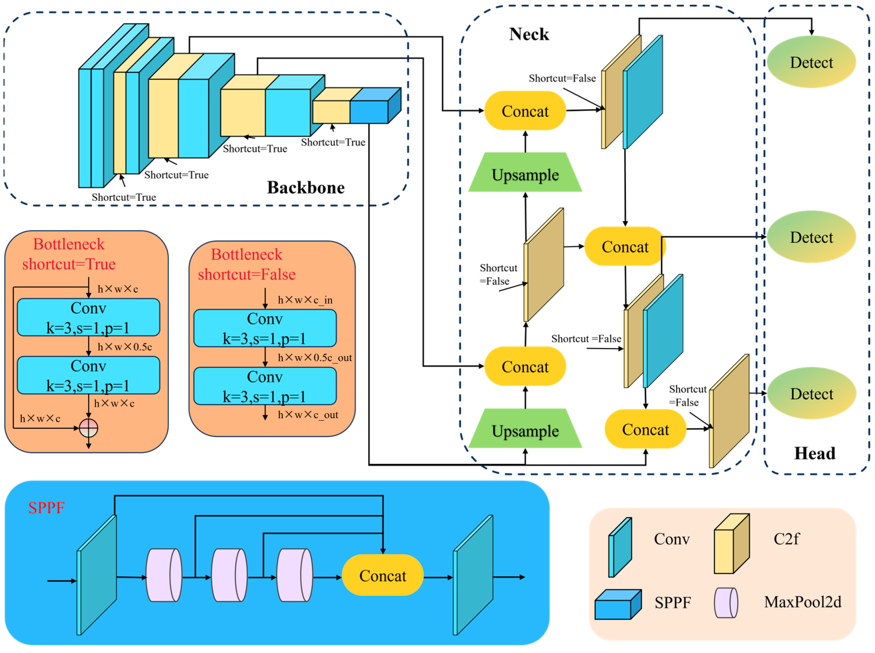
Figure 1. The overall framework of the YOLOv8 network.
Remotesensing 17 03828 g001
Figure 2. The overall framework of the CSBI-YOLO network.
Remotesensing 17 03828 g002
Figure 3. The structure of the Group-Shuffle Feature Enhancement Module (GS-FEM). In channel shuffling, the same-colored blocks and the corresponding arrows represent the information of the same group.
Remotesensing 17 03828 g003
Figure 4. The structure of the Edge-Gated Upsample (EGU).
Remotesensing 17 03828 g004
Figure 5. A visual representation of CIOU and IoU.
Remotesensing 17 03828 g005
Figure 6. Some scene images in the SlewSea-RS dataset.
Remotesensing 17 03828 g006
Figure 7. The performance evolution and comparison of the base model and the improved model during the training phase are depicted in the subplots, with the left subplot comparing the mAP50 values and the right subplot comparing the mAP50–95 values.
Remotesensing 17 03828 g007
Figure 8. The confusion matrices of YOLOv8 and the proposed model on the SlewSea-RS dataset are presented, with the left subplot showing the results of the YOLOv8 model and the right subplot showing the results of the proposed model.
Remotesensing 17 03828 g008
Figure 9. Visualization results of the CSBI-YOLO model and the YOLOv8 model on the SlewSea-RS dataset under different scenarios are presented. Part (A) shows the detection results of YOLOv8, and Part (B) shows the detection results of CSBI-YOLO; the blue bounding box indicates the predicted box.
Remotesensing 17 03828 g009aRemotesensing 17 03828 g009b
Figure 10. The bidirectional grouped bar chart of the F1 score.
Remotesensing 17 03828 g010
Figure 11. Comparison of visualization heatmaps on the SlewSea-RS dataset, the heatmap indicates the activation of the model’s final detection layer, with brighter colors representing higher confidence in the presence of a target at that location.
Remotesensing 17 03828 g011aRemotesensing 17 03828 g011b
Figure 12. Comparison of visualization heatmaps on the DOTA-ship dataset, the heatmap indicates the activation of the model’s final detection layer, with brighter colors representing higher confidence in the presence of a target at that location.
Remotesensing 17 03828 g012aRemotesensing 17 03828 g012b
Figure 13. Collaborative heatmap based on ablation study.
Remotesensing 17 03828 g013
Figure 14. Four-axis line chart based on the ablation study.
Remotesensing 17 03828 g014
Figure 15. Visualization heatmaps after the introduction of different strategies.
Remotesensing 17 03828 g015
Table 1. Configuration and training environment.
ParameterConfiguration
CPU modelIntel Core i7-9700k
GPU modelNVIDIA GeForce RTX 3090Ti
Operating systemUbuntu 18.04 LTS 64-bits
Deep learning framePyTorch 1.9.1
GPU acceleratorCUDA 10.2
Integrated development environmentPyCharm 2024.03
Scripting languagePython 3.8
Neural network acceleratorCUDNN 7.6.5
Table 2. Hyperparametric configuration.
ParameterConfiguration
Neural network optimizerSGD
Learning rate0.001
Training epochs200
Momentum0.937
Batch size32
Weight decay0.0005
Table 3. Comparison of performance metrics for the seven models on the SlewSea-RS dataset.
MethodParam.FLOPSPRmAP50mAP50–95
Fast R-CNN48.585.774.872.277.562.6
Faster R-CNN42.364.177.475.276.163.4
Cascade R-CNN44.675.279.874.680.463.3
YOLOv57.516.883.576.681.162.8
YOLOv811.228.484.379.182.266.3
YOLOv119.622.186.578.485.667.2
DEMNet2.14.588.177.586.470.3
CSBI-YOLO13.330.789.782.688.271.7
Table 4. Comparison of performance metrics for the seven models on the DOTA-ship dataset.
MethodParam.FLOPSPRmAP50mAP50–95
Fast R-CNN48.585.785.983.785.156.2
Faster R-CNN42.364.182.984.485.957.1
Cascade R-CNN44.675.282.680.885.556.4
YOLOv57.516.887.381.986.456.5
YOLOv811.228.485.187.486.661.7
YOLOv119.622.186.886.486.960.9
DEMNet2.14.590.185.685.261.3
CSBI-YOLO13.330.790.584.187.962.7
Table 5. Ablation study based on the SlewSea-RS dataset.
MobileGS-FEMEGUR-IoU-FocalParam.FLOPSPRmAP50mAP50–95FPS
YOLOv8------11.228.484.379.182.266.3106
----13.230.785.480.183.767.595
----11.328.485.279.883.767.3104
----11.228.486.881.584.669.1106
--13.330.787.381.885.469.294
--11.328.487.282.286.169.9104
--13.230.788.682.487.370.895
13.330.789.782.688.271.794
Table 6. Based on the ablation experiments using GS-FEM, the table indicates Convolution followed by channel shuffling with ■, and Channel shuffling followed by convolution with ○, ↓ indicates a decrease, while ↑ indicates an increase.
MobileBranch OneBranch TwoBranch ThreeBranch FourParam.mAP50
GS-FEM--------------
--------------↓ 85%↓ 72%
--------------↓ 86%↓ 79%
------------↓ 61%↓ 55%
------------↓ 62%↓ 63%
----------↓ 6%↓ 8%
------√----↑ 23%↑ 4%
--------↑ 22%↑ 3%
Disclaimer/Publisher’s Note: The statements, opinions and data contained in all publications are solely those of the individual author(s) and contributor(s) and not of MDPI and/or the editor(s). MDPI and/or the editor(s) disclaim responsibility for any injury to people or property resulting from any ideas, methods, instructions or products referred to in the content.