Physics-Informed Deep Learning for 3D Wind Field Retrieval of Open-Ocean Typhoons

Highlights

What are the main findings?

• The proposed physics-informed CNN model, integrating multi-channel satellite data and the continuity equation, reduces MAE in U/V wind components by 29.6% and 21.6% compared to infrared-only baselines.
• The model effectively captures fine-scale typhoon structures such as eyewalls and spiral rainbands while maintaining vertical physical coherence.

What are the implications of the main findings?

• This approach provides a robust, high-resolution 3D wind field retrieval framework for open-ocean typhoons, enhancing real-time monitoring and numerical weather prediction initialization.
• The integration of physical constraints into deep learning models offers a generalizable strategy for improving the dynamical consistency of data-driven meteorological retrievals.

Abstract

Accurate retrieval of three-dimensional (3D) typhoon wind fields over the open ocean remains a critical challenge due to observational gaps and physical inconsistencies in existing methods. Based on multi-channel data from the Himawari-8/9 geostationary satellites, this study proposes a physics-informed deep learning framework for high-resolution 3D wind field reconstruction of open-ocean typhoons. A convolutional neural network was designed to establish an end-to-end mapping from 16-channel satellite imagery to the 3D wind field across 16 vertical levels. To enhance physical consistency, the continuity equation, enforcing mass conservation, was embedded as a strong constraint into the loss function. Four experimental scenarios were designed to evaluate the contributions of multi-channel data and physical constraints. Results demonstrate that the full model, integrating both visible/infrared channels and the physical constraint, achieved the best performance, with mean absolute errors of 2.73 m/s and 2.54 m/s for U- and V-wind components, respectively. This represents significant improvements over the baseline infrared-only model (29.6% for U, 21.6% for V), with notable error reductions in high-wind regions (>20 m/s). The approach effectively captures fine-scale structures like eyewalls and spiral rainbands while maintaining vertical physical coherence, offering a robust foundation for typhoon monitoring and reanalysis.

1. Introduction

Typhoons (also known as tropical cyclones) rank among the most devastating natural disasters, posing severe threats to maritime operations, coastal and geotechnical infrastructure (e.g., slopes [1,2]), and human safety through their intense winds, storm surges, and heavy rainfall [3]. The accurate acquisition of the three-dimensional (3D) wind field structure is fundamental for understanding typhoon dynamics, improving intensity forecasts, assessing wind energy potential [4], and enabling reliable disaster early warning systems [5]. However, obtaining accurate, high-resolution 3D wind fields over the open ocean, where typhoons intensify and evolve, remains a formidable challenge. Traditional in situ observation platforms, such as meteorological masts [6], coastal radars [7], and buoys [8], are spatially sparse, logistically constrained, and often incapacitated under extreme conditions, leading to critical data gaps in the vast oceanic regions [9,10]. While reconnaissance aircraft provide valuable direct measurements, their operations are limited to specific regions and storms, preventing routine global coverage [11]. Numerical Weather Prediction (NWP) models, which assimilate available observations, are consequently hampered by the scarcity of initial 3D wind data over the ocean, negatively impacting the accuracy and lead time of typhoon track and intensity forecasts [12,13].

The advent of satellite remote sensing has partially mitigated this observational void. Geostationary satellites, like the Himawari series, provide continuous, broad-area monitoring with high temporal resolution. Early methods for retrieving surface winds from satellite data relied heavily on empirical models [14] or passive microwave observations [15], but these often lacked the spatial resolution or vertical profiling capability needed to resolve the intricate inner-core structure of typhoons. In recent years, machine learning (ML) has emerged as a powerful tool for establishing complex, non-linear relationships between satellite measurements and geophysical parameters [16]. Techniques such as Random Forest (RF), XGBoost, and Multi-Layer Perceptrons (MLP) have been applied to estimate typhoon parameters, including maximum sustained wind speed and central pressure [17,18,19]. However, MLP suffers from limitations in feature extraction efficiency when handling high-dimensional satellite imagery with strong spatial dependencies [20,21]. Tree-based methods (e.g., RF and XGBoost) are also less effective at capturing the complex spatial structures and textures present in satellite cloud imagery, limiting their ability to resolve typhoon fine-scale features such as eyewalls and spiral rainbands [22,23].

Convolutional Neural Networks (CNNs), with their inherent capabilities for spatial feature learning through local connectivity and weight sharing, have shown considerable promise in meteorological image analysis [24,25]. Several studies have successfully employed CNNs for typhoon-related tasks, such as intensity and size estimation [26,27,28]. Recently, a multi-scale fusion deep learning model for wind field retrieval from geostationary satellite imagery has been proposed [29], and overlapped cloud motion vectors for typhoon monitoring can be obtained using similar data sources [30]. Nevertheless, a significant research gap persists in the retrieval of the complete 3D wind field, which is crucial for understanding the vertical transport of momentum and heat, validating and initializing high-resolution NWP models, and assessing 3D wind loads on structures. Furthermore, most existing ML and CNN models are purely data-driven, learning statistical patterns from training data without explicit guidance from physical laws [31]. This black-box nature can lead to physically implausible results, such as wind fields that violate fundamental principles of fluid dynamics like mass conservation, thereby raising concerns about their generalizability and physical credibility, especially in extreme and dynamically complex regimes like typhoon cores [32,33].

To bridge these critical gaps, this study proposes a physics-informed deep learning framework for the high-resolution 3D reconstruction of open-ocean typhoon wind fields. First, a dedicated CNN architecture that fully leveraged multi-channel data from the Himawari-8/9 geostationary satellites was designed to establish an end-to-end mapping to the complete 3D wind field across 16 vertical levels, addressing the scarcity of methods for holistic 3D retrieval within the lower to middle troposphere, which is critical for many engineering and operational applications, such as marine operations, wind load assessment, and lower-boundary initialization in NWP models. It is recognized that satellite-observed cloud-top features are physically coupled to the dynamics of the entire atmospheric column in an organized system like a typhoon. The CNN does not perform a direct vertical extrapolation but rather learns the complex, statistical-dynamical relationships between these multi-spectral signatures and the concomitant 3D wind field structures. Second, and most importantly, a purely data-driven paradigm was improved by embedding the continuity equation, enforcing mass conservation, directly into the loss function as a strong physical constraint. This compels the model to generate wind fields that are not only statistically accurate but also kinematically consistent, thereby enhancing the physical realism and dynamical coherence of the retrieval results.

2. Materials and Methods

2.1. Himawari-8/9 Satellite Data

Geostationary satellites provide wide coverage and high temporal resolution, making them the primary tools for monitoring tropical cyclones [34]. Himawari satellites, launched by the Japan Meteorological Agency (JMA), offer full-disc observations covering the Northwest Pacific Ocean, including open-ocean typhoon regions. The spectral characteristics of Himawari channels are summarized in Table 1. Visible and infrared channels provide continuous monitoring of cyclone cloud development, while near-infrared channels capture water vapour transport, aiding in identifying typhoon evolution. This study employed visible, near-infrared, and infrared channels obtained from Himawari-8, with 10 min temporal resolution and spatial resolutions of 0.5 km (visible) and 2 km (infrared/near-infrared).

Table 1. Himawari series satellites full-disc channel parameters.

Channel Number	Channel Type	Channel Band	Frequency	Range
1~3	Visible light	0.46~0.64 μm	10 min	60°S–60°N 80°E–160°W
4~6	Near-infrared	0.86~2.3 μm
7~16	Infrared	3.9~13.3 μm

Figure 1 shows the albedo data obtained from the visible light and near-infrared channels of the satellite at a moment during an open-ocean typhoon, and Figure 2 shows the brightness temperature data derived from infrared channels at the same time. Both figures are centred on the typhoon centre and covers a 10° × 10° area in latitude and longitude. Following figures are presented in the same manner. Channels 1–3 are visible light channels, which mainly observe the reflected light from the ground surface; Channels 4–6 are near-infrared channels, which mainly observe cloud particle size and phase; Channels 7–10 are short wave infrared channels, which mainly observe the amount of water vapour; Channels 11–13 are sub infrared channels, which mainly identify the cloud phase; Channels 14–16 are ultra infrared channels, which mainly observe the sea surface water temperature and cloud height. It can be seen from figures that the overall brightness temperature increases with the increase in the wavelength of the channel. Based on the date from 16 channels, a small and round eye area can be observed in the centre of the typhoon, and there is a close and relatively low temperature area around, indicating that the typhoon has extremely high intensity. Comparison of Figure 1 and Figure 2 suggests that the typhoon structure reflected by different channels is significantly different and complementary due to their different physical characteristics. The visible light channel can clearly show the fine texture and morphological characteristics of the cloud system, while the infrared channel highlights the cloud top height and thermal structure characteristics through the brightness temperature distribution, especially in the identification of strong convection zone and eye wall thermal gradient. The observation characteristics of multi-dimensional and multi physical quantities provide a rich source of information for the comprehensive analysis of the three-dimensional dynamic structure of typhoon. Therefore, the fusion of multi-channel satellite data and the comprehensive utilization of their complementary information play an important role in improving the accuracy and integrity of 3D wind field inversion.

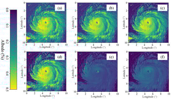
Figure 1. Himawari-8 visible and near-infrared channel image obtained from (a) Chanel 1; (b) Chanel 2; (c) Chanel 3; (d) Chanel 4; (e) Chanel 5; (f) Chanel 6.

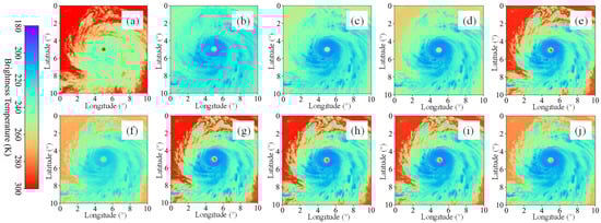
Figure 2. Himawari-8 infrared channel image obtained from (a) Chanel 7; (b) Chanel 8; (c) Chanel 9; (d) Chanel 10; (e) Chanel 11; (f) Chanel 12; (g) Chanel 13; (h) Chanel 14; (i) Chanel 15; (j) Chanel 16.

2.2. ERA5 Reanalysis Wind Field Dataset

The ground-truth wind field data were obtained from the ERA5 reanalysis dataset provided by the European Centre for Medium-Range Weather Forecasts (ECMWF). ERA5, which assimilates all available observations into a physically consistent model, currently provides the complete and globally available representation of the 3D atmospheric state, making it a widely adopted benchmark for studies of this nature. While using reanalysis for both training and evaluation may introduce potential biases, the primary objective of this study is to perform a controlled comparison of different model configurations under a consistent benchmark. The dataset has a spatial resolution of 0.25° × 0.25° and a temporal resolution of 1 h, featuring 37 vertical pressure levels. For this study, U- and V-wind speed components at 16 height levels (ranging from 110 to 5550 m) were selected as labels for the CNN model. This vertical domain was deliberately chosen to align with the primary sensitivity of the employed Himawari visible and infrared channels and to focus on the wind field layers most relevant to the maritime operations, coastal engineering, and wind energy assessment. These pressure levels were converted to height levels using the following universal pressure–height equation:

$$H=44300\left[1-{\left({\displaystyle \frac{P}{1013.25}}\right)}^{{\displaystyle \frac{1}{5.256}}}\right]$$

(1)

where H denotes the height above mean sea level in metres; P denotes the pressure at the target height in hPa. The international standard sea-level (H corresponding to 0 m) pressure is 1013.25 hPa. Figure 3 presents the horizontal wind field from the ERA5 reanalysis dataset at six representative height levels, clearly revealing the vertical stratification of the typhoon’s 3D wind structure. A comparison of the wind fields across different heights demonstrates the variation in wind speed and direction with altitude.

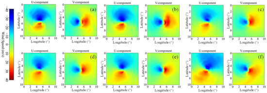
Figure 3. Wind field of Typhoon Chan-hom at 00:00 UTC on 7 July 2015 across different heights from ERA5: (a) 5550 m; (b) 4200 m; (c) 3000 m; (d) 2000 m (e) 1000 m; (f) 110 m.

2.3. Typhoon Data Preprocessing

A total of 790 representative typhoons over the Northwest Pacific from 2015 to 2023 were selected as the total dataset for this study. To ensure the model learns from well-developed vortex structures, our dataset specifically samples from typhoon systems that have reached an intensity of ‘Typhoon’ or higher (Level 4 and above) according to the CMA classification, encompassing ‘Typhoon’, ‘Severe Typhoon’, and ‘Super Typhoon’ categories. The distribution of the maximum sustained wind speed (MSW) from the CMA best-track dataset for all samples is provided in Figure 4, confirming the coverage of high-intensity systems relevant for extreme wind retrieval.

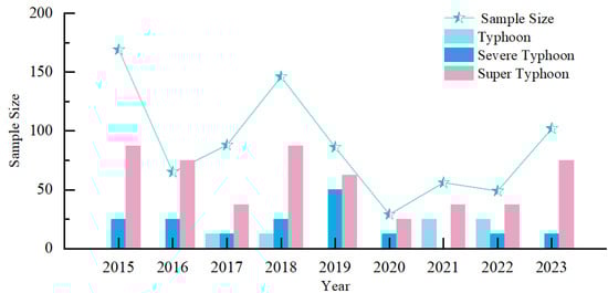
Figure 4. Distribution of typhoon intensity in the dataset.

To standardize the spatial scale and structure, both the satellite and ERA5 datasets were re-gridded onto a typhoon-centred coordinate system, generating 3D wind field samples covering a 10° × 10° area with a spatial grid of 41 × 41 pixels and 16 vertical levels. This grid configuration provides sufficient spatial detail to resolve the macroscopic structure of key typhoon features such as the eyewall and spiral rainbands for the purpose of error analysis, which is conducted by comparing model predictions directly against the ERA5 wind fields on this common grid. The typhoon centre positions were obtained from the China Meteorological Administration (CMA) best-track dataset [35] and were used to align the centres in both the Himawari-8/9 satellite imagery and the reanalysis data. Centred on the typhoon eye, the Himawari-8/9 data were cropped to 501 × 501 pixels, covering a radius of 500 km approximately. A small number of missing satellite values were filled using linear interpolation from adjacent pixels. The corresponding ERA5 reanalysis wind fields were gridded into 41 × 41-pixel images. Figure 5 depicts the distribution of the processed reanalysis wind speeds, with the horizontal axis showing the wind speed and the vertical axis showing its frequency of occurrence. The dataset primarily covers wind speeds ranging from 0 to 40 m/s, reflecting the comprehensive statistical characteristics of 790 typhoon samples over the Northwest Pacific. It is important to note that this histogram represents the frequency of wind speed values across all samples and locations, not an upper limit for the model. The model is trained on and capable of predicting higher wind speeds, as evaluated in Section 3.

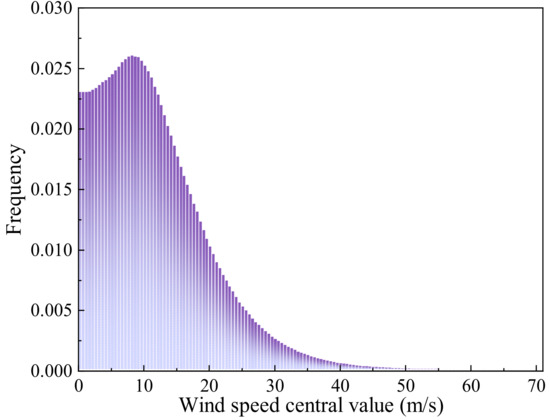
Figure 5. Wind speed distribution.

Figure 6 displays the processed mean wind speed at each height level, which peaks at approximately 12.24 m/s around 1250 m, indicating the characteristic wind speed maximum near the top of the atmospheric boundary layer during typhoon conditions. To prevent gradient vanishing or explosion and to enhance training efficiency, a Min-Max normalization [36] below, suitable for data relatively concentrated, was employed to scale all feature variables to a consistent range:

$$x={\displaystyle \frac{x_0-x_{min}}{x_{max}-x_{min}}}$$

(2)

where $x_0$ is the original Himawari-8/9 data; $x_{max}$ and $x_{min}$ represent the maximum and minimum values of the sample data, respectively; and $x$ denotes the consistently formatted data after transformation, which is scaled to the range from 0 to 1 for use as neural network input.

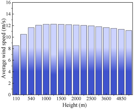
Figure 6. Processed mean wind speed across different height levels.

2.4. Typhoon Retrieval Scenarios

To ensure a robust and unbiased evaluation of model performance and to mitigate potential biases from a single data split, a 10-fold cross-validation strategy was employed. In each fold, 80% of the data was used for training, 10% for validation, and 10% for testing. This process was repeated 10 times, and all reported performance metrics represent the average across these 10 independent trials. To prevent any potential data leakage, the dataset was partitioned at the typhoon-case level, ensuring that all samples originating from the same typhoon were assigned exclusively to a single fold. Consequently, no temporal segments or spatial patches from the same typhoon appeared simultaneously in both the training and testing subsets. This case-wise separation guarantees that the model is evaluated on entirely unseen typhoon events, thereby providing a realistic assessment of its generalization capability under operational conditions. Four distinct experimental scenarios, as outlined in Table 2, were designed, employing a controlled variables approach to systematically evaluate the contribution of each component. The baseline scenario design was motivated by operational meteorological requirements. Since infrared channels provide continuous all-weather coverage, unlike visible channels which are unavailable during nighttime, B1 and B2 were established as infrared-only baselines. The scenarios B3 and B4, which incorporate visible channels, were developed to evaluate the incremental improvement from multi-spectral fusion under a realistically constrained (i.e., daytime-only) scenario. While a direct comparison between infrared-only and visible-only models is insightful, it is inherently constrained by data availability, as any visible-only model can only be trained and evaluated on approximately half of the dataset (daytime scenes), whereas an operational system has to perform under all-sky conditions.

Table 2. Experimental scenario design for 3D wind-field retrieval.

Scenarios	Input	Physical Constraint
B1	Infrared channels (9–16)	×
B2	Infrared channels (9–16)	✓
B3	Infrared + visible channels (1–16)	×
B4	Infrared + visible channels (1–16)	✓

2.5. Convolutional Neural Network Construction

The fundamental unit of a neural network is the neuron [37]. Each neuron receives input signals, multiplies them by corresponding weights, adds a bias term, and applies an activation function to generate the output, which can be expressed using the following equation:

$$y=\mathsf{\phi }\left({\sum }_i\left({\omega }_i\times x_i\right)+b\right)$$

(3)

where $x_i$ denotes the input, ω the weights, $b$ the bias, $\mathsf{\phi }$ the activation function, and $y$ the neuron’s output processed by the activation function. Convolutional Neural Networks are effective at hierarchical feature learning. Typically, CNNs comprise convolutional, pooling, and fully connected layers. Through successive convolution and pooling operations, CNNs capture multi-scale spatial features and construct increasingly abstract representations of the input [38]. The convolution operation can be formalized in the following equation:

$$z\left(x,y\right)=(f\ast g)(x,y)={\sum }_m{\sum }_{n}f\left(x-m,y-n\right)g\left(m,n\right)$$

(4)

where $f\left(x,y\right)$ represents the input satellite image, $g\left(m,n\right)$ denotes the two-dimensional convolution kernel with spatial offsets (m, n), $(f\ast g)(x,y)$ explicitly represents the discrete convolution operation between functions f and g evaluated at position (x, y), using standard mathematical notation that avoids ambiguity present in the previous formulation, and $z\left(x,y\right)$ is the output feature map.

Figure 7 presents the specific CNN architecture used in this work, where “Conv” denotes convolutional layers and the output layer predicts the surface wind field. The network comprises 11 convolutional layers, 5 pooling layers, 1 fully connected layer, and 1 output regression layer. All activation functions use ReLU to mitigate vanishing gradients. Input data size and channels, convolution kernel sizes and numbers, pooling strides, and output nodes are summarized in Table 3. To optimize the network training process, the following key hyperparameters and training strategies were adopted: Stochastic Gradient Descent (SGD) was used as the optimizer with a base learning rate of 0.001 and a batch size of 8. The maximum training epoch was set to 500, while an early stopping mechanism was implemented during actual training to prevent overfitting. The model was implemented using the TensorFlow/Keras framework, and L2 weight regularization (coefficient 0.001) was introduced in all convolutional and fully connected layers to enhance generalization capability. This parameter combination demonstrated the best balance between convergence speed and stability in preliminary experiments.

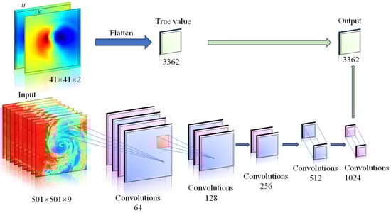
Figure 7. Structure of deep learning model.

Table 3. Configuration parameters of the convolutional neural network architecture.

Structure	Design Content
Input layer	Receives Himawari-8/9 9/16-channel infrared data (501 × 501 pixels)
Feature extraction module	4 convolutional layers with 64 kernels of size 3 × 3 → MaxPooling (2 × 2, stride 2)
	3 convolutional layers with 128 kernels of size 3 × 3 → MaxPooling (2 × 2, stride 2)
	2 convolutional layers with 256 kernels of size 3 × 3 → MaxPooling (2 × 2, stride 2)
	1 convolutional layer with 512 kernels of size 3 × 3 → MaxPooling (2 × 2, stride 2)
	1 convolutional layer with 1024 kernels of size 3 × 3 → MaxPooling (2 × 2, stride 2)
Feature decoding module	Fully connected layer (1024 neurons)
Output layer	Regression output for wind field (U/V components, total 3362 nodes)

The core capability of the proposed CNN architecture lies in its ability to learn the complex, non-linear statistical relationships and physical associations between multi-channel satellite-observed cloud-top features and the three-dimensional wind field structures provided by ERA5 as labels. Through extensive training on a large dataset of typhoon cases, the deep convolutional layers hierarchically extract spatial patterns from the satellite imagery that are diagnostically linked to the underlying dynamic processes governing the wind field from the surface up to 5550 m.

2.6. Loss Function

To better capture the strong-wind regions in the typhoon core, the main loss function incorporates an exponential weight that depends on wind speed. This design mitigates the equal weighting of errors in conventional loss functions such as mean squared error (MSE), which treat high- and low-speed regions identically. By assigning larger penalties to errors at higher wind speeds, the weighted loss enhances the model’s sensitivity to extreme conditions. The mathematical form is expressed as

$${\mathcal{L}}_{main}={\displaystyle \frac{1}{N}}{\sum }_1^N\left(e\times \left|y_t-y_p\right|\times a^{\left|y_t\right|}+\left(1-e\right)\times \left|y_t-y_p\right|\right)$$

(5)

where ${\mathcal{L}}_{main}$ denotes the main loss, and N the batch size; $y_t$, $y_p$ are true and predicted wind speeds, respectively; Parameter e is used to smooth potential numerical instability when wind speed approaches zero; parameter a (a > 1) controls the enhancement degree of error penalties for large wind speeds. The larger a is, the heavier the penalty on high-wind errors. After a series of trail runs, e and a were set to 0.1 and 1.1, respectively.

In 3D typhoon wind field retrieval, relying exclusively on data-driven models may fail to ensure that the results conform to fundamental fluid dynamics principles [39]. To enhance the physical consistency of the model, this study innovatively incorporates the continuity equation as a strong physical constraint into the loss function. For large-scale atmospheric motions, particularly at the higher levels within the retrieved vertical range (e.g., around 4850 m), the flow can be approximated as incompressible under the quasi-hydrostatic balance and Boussinesq approximation [40]. Accordingly, the divergence of the velocity field is zero, which means it must satisfy the following continuity equation:

$$\nabla ·V=0$$

(6)

This implies zero net flux in/out of a unit volume. On a discrete 2D horizontal grid, this can be applied to horizontal wind components $u$ and $v$:

$$div={\displaystyle \frac{\partial u}{\partial x}}+{\displaystyle \frac{\partial v}{\partial y}}$$

(7)

The physical constraint is implemented as follows. First, the model’s predicted output was reshaped into a 2D wind field grid of size 41 × 41, from which u and v are extracted. Next, the spatial gradients of these components, ∂u/∂x and ∂v/∂y, were computed using the central difference method. According to the definition of divergence in fluid dynamics, the divergence field was obtained as the sum of these gradients. The mean squared divergence was then used as the physical constraint term. A weighting coefficient λ was introduced to balance the contributions of the data-fitting loss and the physical constraint. Thus, when physical enhancement was incorporated, the total loss function consists of two components: a primary loss and a physical constraint term. The primary loss adopted a weighted absolute error form that applied exponential weighting to amplify the penalty on large errors while preserving sensitivity to small errors. The physical constraint term ensured the flow field satisfies the divergence-free condition by minimizing the divergence. The complete loss function is given in Equation (8):

$$\mathcal{L}={\mathcal{L}}_{main}+\lambda ·{\mathcal{L}}_{phys}$$

(8)

where ${\mathcal{L}}_{phys}$ is the divergence constraint term and λ is the weight coefficient (=0.1 in this study).

Loss functions based on conventional parameters, such as Mean Absolute Error (MAE), mean squared error (MSE), and root-mean-square error (RMSE) [41], while capable of measuring the overall error level in wind field retrieval, impose equal penalties for errors in both high- and low-wind-speed regions, making it difficult to adequately reflect the importance of extreme winds in the typhoon core.

Table 4 compares the performance of different loss functions for retrieving the 10 m wind field using satellite infrared channel data. As shown in the table, the average errors differ only slightly among the four loss functions, with the RMSE-based loss yielding the largest errors in the U and V components. However, when the wind speed range is increased to above 20 m/s, the differences become markedly pronounced: the custom loss function achieves U and V component errors of 3.83 m/s and 4.01 m/s, respectively, which are significantly lower, by over 20%, than those of MSE and RMSE. Compared with MAE, the custom loss also maintains an advantage of approximately 5%. This indicates that MSE and MAE tend to balance errors across the entire field, whereas the exponential weighting in the proposed loss function amplifies the penalty for high-wind-speed errors, thereby substantially improving the retrieval accuracy of strong winds in the typhoon core region.

Table 4. Error of retrieval using different loss functions.

Speed	Custom	MSE	MAE	RMSE
U average	2.23	2.30	2.23	2.94
V average	2.24	2.29	2.22	2.77
U: >20 m/s	3.83	5.05	4.04	5.65
V: >20 m/s	4.01	5.03	4.24	5.00

3. Results

To systematically verify the reliability of the proposed physics-informed deep learning model, this study evaluates results from three perspectives: quantitative wind-speed error metrics, spatial error distribution of the wind field, and typical typhoon case analyses.

The error metrics for different experimental scenarios are summarized in Table 5. For the average wind speed error, the B1 model, using only infrared input, achieved MAE of 3.88 m/s and 3.24 m/s for the U- and V-components, respectively. Introducing the continuity equation constraint in model B2 reduced these errors to 3.26 m/s and 2.68 m/s, corresponding to reductions of 16.0% and 17.3%, which confirms the effectiveness of physical regularization in suppressing spurious fluctuations. Model B3, which further incorporated visible channel data, compressed the U and V errors to 2.94 m/s and 2.75 m/s, close to the performance of B2, indicating that multispectral texture information also contributes significantly to error suppression. Finally, the full model B4, combining both visible channels and physical constraints, achieved MAEs of 2.73 m/s and 2.54 m/s for the U- and V-components, respectively. These values correspond to a 29.6% and 21.6% improvement over B1 and still show a further 6.8% and 2.5% reduction compared to B3, fully demonstrating the synergistic advantage of “data fusion + physical regularization”.

Table 5. Error of retrieval with different loss functions.

Speed	MAE-B1: m/s	Error-B1: %	MAE-B2: m/s	Error-B2: %	MAE-B3: m/s	Error-B3: %	MAE-B4: m/s	Error-B4: %
Average U	3.88	29.43	3.26	25.94	2.94	22.17	2.73	20.72
Average V	3.24	25.13	2.68	21.00	2.75	22.71	2.54	19.40
U: 5–10 m/s	3.10	42.60	2.49	32.91	2.47	32.63	2.57	33.99
V: 5–10 m/s	2.65	36.88	2.55	34.56	2.49	33.66	2.11	28.35
U: 10–15 m/s	3.31	26.94	2.75	22.44	2.45	20.03	2.48	18.18
V: 10–15 m/s	2.81	22.84	2.49	19.93	2.52	20.74	2.15	17.45
U: 15–20 m/s	4.38	25.36	3.88	22.59	3.25	19.03	2.91	17.02
V: 15–20 m/s	3.64	21.13	3.08	17.93	3.26	19.04	2.86	16.70
U: >20 m/s	5.73	22.88	5.80	22.76	4.36	16.96	4.03	16.03
V: >20 m/s	4.93	19.66	4.54	18.22	4.45	17.38	4.07	16.37

To evaluate performance across different wind speed regimes, Table 5 categorizes the four experimental scenarios into the following intervals: >20 m/s, 15–20 m/s, 10–15 m/s, and 5–10 m/s. The results reveal that in the >20 m/s range, B2 showed negligible improvement in the U-component compared to B1, while the V-component error decreased to 4.54 m/s, indicating that the continuity constraint alone had a limited suppression effect in the high-wind core region when only infrared data is available. In contrast, the introduction of visible channels in B3 leaded to substantial error reduction in this interval, with U- and V-component errors decreasing by 23.9% and 9.7%, respectively, relative to B1. This suggests that under high-wind conditions, cloud-top texture and convective structural information from visible imagery played a critical role in suppressing retrieval errors. Further integrating the physical constraint in B4 reduced U- and V-errors to 4.03 m/s and 4.07 m/s, corresponding to additional reductions of 7.6% and 8.5% compared to B3. This confirms that the combination of multi-channel input and physical regularization provided secondary gains even in extreme wind speed intervals. In the 15–20 m/s range, B4 achieved U- and V-errors as low as 2.91 m/s and 3.08 m/s, representing improvements of 33.6% and 15.4% over B1. A similar trend was maintained in the 10–15 m/s and 5–10 m/s intervals, where B4 consistently yielded the lowest errors, and the relative contribution of the physical constraint gradually increased as wind speed decreased. In summary, accuracy gains in the high-wind regime relied primarily on the inclusion of visible-channel textures, whereas the mid- to low-wind regimes benefitted more markedly from physical regularization. Together, these two components formed a complementary strategy that enhanced retrieval accuracy across all wind speeds.

Figure 8 displays the validation loss curves for the four scenarios. The B1 configuration shows the steepest initial decline within the first 100 epochs, whereas B4 eventually converges to the lowest and most stable validation loss value. This behaviour demonstrates the positive effect of the continuity equation constraint in guiding the training process, thereby mitigating overfitting and enhancing learning stability.

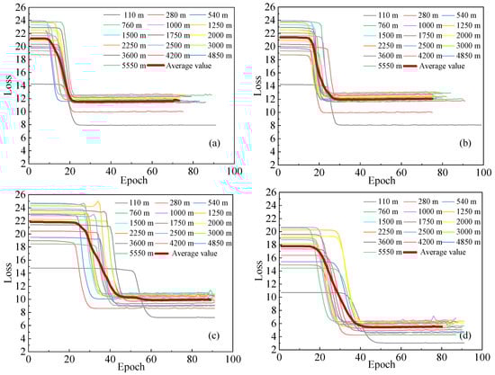
Figure 8. Validation loss curves of four scenarios across different height levels: (a) B1; (b) B2; (c) B3; (d) B4.

Figure 9 presents the Global Mean Absolute Error (GMAE) calculated over the entire test set at a certain height level, illustrating the variation in average U/V-component errors across different heights. It can be observed that models B3 and B4 achieved lower errors at most height levels, in both the lower (110–1500 m) and middle-to-upper (2500–5550 m) layers, while the error generally increased with altitude. This trend reflects the greater continuity and predictability of wind fields in the middle and lower atmosphere and also indicates the model’s stronger capability in identifying structural features in regions of strong winds at these heights.

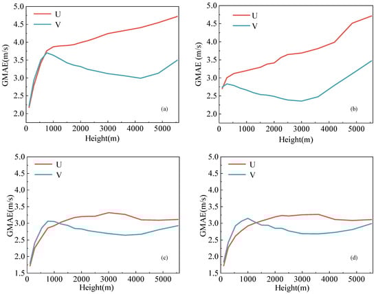
Figure 9. GMAE in U- and V- directions of four scenarios across different height levels: (a) B1; (b) B2; (c) B3; (d) B4.

To further characterize model stability across different pressure levels, Figure 10 presents the relative error distributions of the four scenarios at each of the 16 height layers. The mean error of all schemes increased monotonically with height, peaking at 5550 m and reaching its lowest value at 110 m, indicating greater uncertainty in upper-level wind fields. In comparison, B2 consistently achieved lower errors than B1 across all heights, approximately 5% at 110 m and about 32% at 5550 m, demonstrating that the physical constraint alone reduced errors by roughly 6–8% on average. Relative to B1, B3 attained a 32.4% reduction in error at 5550 m, confirming that visible channels also contributed to retrieval accuracy. B4 consistently yielded the lowest errors across all layers: its performance at 110 m was comparable to the other models, while at 5550 m it achieved an error of about 24%. These results highlight the ability of multispectral data to reduce overall errors and the particular role of physical constraints in mitigating errors at higher altitudes. Overall, B4 maintained the lowest mean error and the smallest inter-layer variability across all pressure levels, verifying that the integration of visible channels and continuity equation constraints improved both the accuracy and vertical consistency of 3D wind field retrievals in a top-down manner.

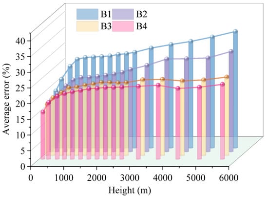
Figure 10. Error distribution of different pressure layers.

In summary, the proposed CNN model (B4), which integrates physical constraints with multi-channel data, outperforms conventional data-driven approaches in overall error control, mid-to-high-level accuracy consistency, and model stability. The model already demonstrates strong potential in retrieving physically consistent 3D wind-field structures with high predictive accuracy, thereby laying a solid foundation for future high-resolution, physically consistent reanalysis of typhoon wind fields over the open ocean. While the proposed model demonstrates significant improvements over baseline approaches, the retrieval of the most extreme wind speeds within the typhoon core (e.g., sustained winds significantly above 20 m/s) remains a challenging frontier. This challenge is multifaceted, arising from the inherent scarcity of such extreme events in training data and the potential saturation of optical and infrared satellite signals under the most intense convective conditions, decoupling cloud-top features from surface winds. Future research can integrate complementary satellite data to addressing these challenges.

4. Discussion

The spatial distribution of wind field errors serves as a key indicator for evaluating the physical consistency of a retrieval model. Figure 11 shows an example of the predicted and ground-truth wind fields at multiple height levels produced by the physics-informed model B4. It is visually evident that the discrepancy between prediction and truth diminishes at lower altitudes, a finding that aligns with and corroborates the quantitative error analysis presented earlier.

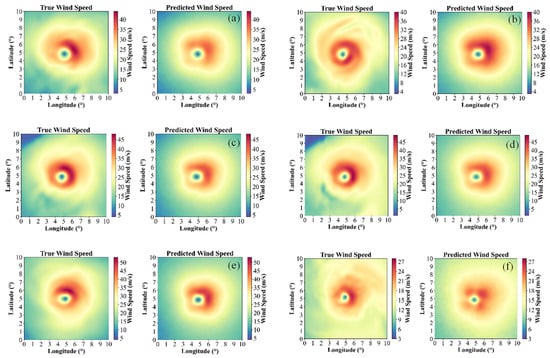
Figure 11. Comparison between true and predicted wind speeds across different heights: (a) 5550 m; (b) 4200 m; (c) 3000 m; (d) 2000 m; (e) 1000 m; (f) 110 m.

Figure 12 presents the averaged error distributions in both zonal and meridional directions across 16 vertical layers for the four experimental scenarios. It is important to reiterate that these patterns are derived from the model’s learned statistical mapping and are evaluated against the ERA5 wind fields on this common grid. The physical constraint of mass conservation further guides this mapping, promoting kinematically consistent vertical structures and enhancing the physical realism of the retrieved wind fields in these dynamically critical regions. The structure of the true wind field reveals pronounced wind speed gradients within the typhoon core region, in contrast to the relatively gentle gradients in the outer area. The B1 model exhibited a “high-in-core, low-in-periphery” error pattern in both zonal and meridional components: within the eyewall region (approximately 4–6° in latitude), the mean vector wind speed error reached 5 m/s, with the U-component error peaking around latitude 5° (5.3 m/s) and the V-component error reaching its maximum in the same latitudinal zone (4.7 m/s). These patterns corresponded to the sharp wind variations caused by intense rotational flows in the eyewall, indicating that purely data-driven models struggle to capture flow continuity in regions with strong gradients. In comparison, the B2 model shows a notable contraction of errors in the core region: within the same 4–6° latitudinal eyewall band, the vector wind speed error decreased to 4.5 m/s, and the peak errors in the U- and V-components were reduced by 4% and 10%, respectively. This demonstrates that the physical constraint, by enforcing a divergence-free condition, effectively suppressed unphysical error propagation in high-gradient regions.

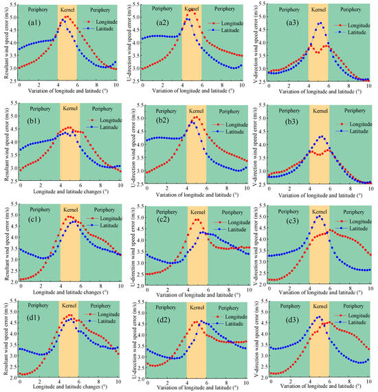
Figure 12. Error distribution along longitude and latitude directions: (a1) resultant wind speed of B1 scenario; (a2) U-direction wind speed of B1 scenario; (a3) V-direction wind speed of B1 scenario; (b1) resultant wind speed of B2 scenario; (b2) U-direction wind speed of B2 scenario; (b3) V-direction wind speed of B2 scenario; (c1) resultant wind speed of B3 scenario; (c2) U-direction wind speed of B3 scenario; (c3) V-direction wind speed of B3 scenario; (d1) resultant wind speed of B4 scenario; (d2) U-direction wind speed of B4 scenario; (d3) V-direction wind speed of B4 scenario.

The error distribution of model B3 shows improvement over that of B1, particularly in the reduction in error peaks near the typhoon eyewall. However, the errors in the eyewall region remained relatively high, indicating that, in the absence of physical constraints, the model still had limitations in handling extreme wind gradients. In contrast, the B4 model achieved further improvement in error distribution, with its peak errors near the eyewall being lower than those of B3. While the averaged error profiles in Figure 12d1–d3 show that B4’s error in the core region is comparable to or occasionally slightly higher than that of B2, the quantitative metrics in Table 5 confirm that B4 achieves the lowest overall errors in the high-wind speed regime (>20 m/s). This suggests that the B4 scenario provides the most robust and accurate retrieval when considering the entire domain and all wind regimes, even if the physical constraint’s smoothing effect in the extreme core is, in this visualization, similarly effective to the B2 scenario which uses a different information base. This result highlights the critical role of the physical constraint in enhancing prediction accuracy, especially in regions with strong wind speed gradients. By enforcing a divergence-free condition on the flow field, the physical regularization effectively suppressed unphysical error propagation, thereby improving the model’s stability and accuracy under extreme conditions.

Figure 13 reveals detailed spatial average errors across 16 layers for the four experimental scenarios. All models show a consistent pattern where errors peaked in the central region and decreased toward the periphery. In the B1 model, the largest average errors were concentrated in the area where the outer eyewall interacts with spiral rainbands (approximately 4–6° in both latitude and longitude). With the introduction of the physical constraint in model B2, the maximum average errors were reduced by 9.8%, 16.9%, and 1.6% for the vector wind, U- and V-component, respectively, while spatial continuity was markedly improved. Model B3 achieved a further reduction in maximum average error through the incorporation of visible channels. By integrating both visible channels and physical constraints, model B4 exhibited the best error characteristics: its maximum average errors (approximately 8.64 m/s for vector wind, 8.86 m/s for U-component, and 6.74 m/s for V-component) were the lowest among all models, its error distribution was more uniform, and no prominent high-error areas remained. These results clearly demonstrate that the combination of multi-channel data fusion and physical constraints significantly enhances both the spatial accuracy and consistency of wind field retrieval.

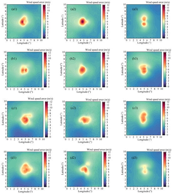
Figure 13. Spatial distribution of error in: (a1) resultant wind speed of B1 scenario; (a2) U-direction wind speed of B1 scenario; (a3) V-direction wind speed of B1 scenario; (b1) Resultant wind speed of B2 scenario; (b2) U-direction wind speed of B2 scenario; (b3) V-direction wind speed of B2 scenario; (c1) resultant wind speed of B3 scenario; (c2) U-direction wind speed of B3 scenario; (c3) V-direction wind speed of B3 scenario; (d1) resultant wind speed of B4 scenario; (d2) U-direction wind speed of B4 scenario; (d3) V-direction wind speed of B4 scenario.

5. Conclusions

This study developed and validated a physics-informed deep learning framework for retrieving the three-dimensional wind field structure of open-ocean typhoons. The research effectively addresses two critical gaps in the current state of the art: the scarcity of methods for full 3D wind field retrieval and the physical inconsistency of purely data-driven models. The findings systematically demonstrate that the synergistic integration of multi-channel satellite data and fundamental physical laws leads to superior accuracy, robustness, and physical realism in the retrieved wind fields.

The core of the proposed methodology is a deep Convolutional Neural Network (CNN) that leverages the rich spatial and spectral information from 16 channels of Himawari-8/9 satellite data. The network was designed to directly map these inputs to the U and V components of the wind across 16 vertical levels, creating a comprehensive 3D output. By moving beyond conventional metrics like MAE, a custom, wind-speed-weighted loss term was introduced to prioritize accurate retrieval in the high-wind-speed core of the typhoon, where errors are most critical. More importantly, the continuity equation, representing mass conservation for large-scale atmospheric flow, was embedded as a physical constraint term. This forces the model to learn solutions that are not merely statistically plausible but also kinematically consistent, effectively acting as a regularizer against physically implausible predictions.

The experimental design, comprising four scenarios (B1 to B4), allowed for a rigorous, controlled evaluation of each component’s contribution. The comparison between Scenario B1 (infrared only) and B3 (visible + infrared) clearly shows that incorporating visible channels substantially enhances retrieval accuracy. The textural and morphological information from visible imagery is particularly valuable for resolving fine-scale features in the typhoon’s core, such as the eyewall and inner rainbands. This led to a marked reduction in errors, especially in the high-wind-speed regime (>20 m/s), where cloud-top texture provides crucial cues on underlying dynamics; The improvement from Scenario B1 to B2 (infrared with physical constraint) demonstrates that even with a limited input dataset, enforcing physical laws yields significant benefits. The continuity equation constraint effectively suppressed spurious fluctuations and unphysical divergences, reducing errors by approximately 16–17% on average for the infrared-only case. This was especially evident in the spatial error analysis, where the “high-in-core, low-in-periphery” error pattern of the purely data-driven B1 model was notably mitigated in B2, leading to smoother and more coherent wind fields, particularly in high-gradient regions; Scenario B4, which combines the full suite of multi-spectral inputs with the physical constraint, consistently outperformed all other models across all evaluation metrics. It achieved the lowest Mean Absolute Errors (2.73 m/s for U, 2.68 m for V), the most stable training convergence, and the most uniform spatial error distribution. The model excelled across all wind speed intervals and vertical layers. Notably, in the high-wind core, the multi-spectral data provided the primary source of improvement, while the physical constraint offered a secondary, yet significant, gain in accuracy and stability. In mid-to-low wind speeds and at higher altitudes, the physical constraint played a more dominant role in enhancing performance; The analysis of errors across different heights revealed that the B4 model maintained the lowest and most consistent error profile from the surface up to 5550 m. While all models exhibited increased uncertainty with altitude, the integration of physical knowledge in B4 substantially curbed this growth, confirming that the physics-informed approach is crucial for generating reliable, vertically coherent 3D structures.

In summary, this research establishes that the path toward reliable, high-resolution 3D typhoon wind field retrieval lies in a hybrid approach that seamlessly blends the powerful pattern recognition capabilities of deep learning with the governing laws of fluid dynamics. The proposed model moves beyond a “black box” approximation to become a physically aware system, resulting in retrievals that are both accurate and dynamically consistent. While there remains room for further improvement, particularly in capturing the absolute extremes of the most intense typhoons, this work lays a solid foundation for future research and applications. The generated high-resolution, physically consistent 3D wind fields can directly contribute to improving typhoon initial conditions for numerical weather prediction models, enhancing real-time monitoring and intensity forecasting, and supporting detailed risk assessment for marine and coastal engineering. As this study focused on the lower-to-mid tropospheric wind field, a recognized limitation is the exclusion of the upper troposphere, which precludes the model from capturing the complete vertical dynamic profile, including upper-level outflow. Future work will prioritize extending the vertical domain of the retrieval to cover the entire troposphere (e.g., up to 100 hPa) using the full vertical levels available in ERA5. This will allow the model to fully leverage satellite-observed cloud-top information for inferring winds throughout the atmospheric column. Future work can also incorporate additional physical constraints (e.g., the vorticity equation) and independent observations (e.g., SAR-derived surface winds) to better capture the balanced dynamics and evolution of the typhoon vortex, and to conclusively demonstrate absolute accuracy and generalizability of retrieved 3D wind fields.

References

- Zhang, W.; Ali, M.; Cui, W.; Sun, C.; Zheng, Z.; Chen, K. Severe Rainfall—Induced Landslides in Pingyuan. Landslides 2025, 22, 2623–2639. [Google Scholar] [CrossRef]
- Cui, W.; Chen, K.; Qing, Z.; Zheng, Z.; Zhang, W.; Zhou, Z.; Han, P.; Zhang, J.; Zhu, Z.; Sun, C. Interpretable Machine Learning Incorporating Major Lithology for Regional Landslide Warning in Northern and Eastern Guangdong. NPJ Nat. Hazards 2025, 2, 89. [Google Scholar] [CrossRef]
- Yu, L.; Qin, H.; Wei, W.; Ma, J.; Weng, Y.; Jiang, H.; Mu, L. Storm Surge Risk Assessment Based on LULC Identification Utilizing Deep Learning Method and Multi-Source Data Fusion: A Case Study of Huizhou City. Remote Sens. 2025, 17, 657. [Google Scholar] [CrossRef]
- Zhang, F.; Dong, Y.; Zhang, K. A Novel Combined Model Based on an Artificial Intelligence Algorithm-A Case Study on Wind Speed Forecasting in Penglai, China. Sustainability 2016, 8, 555. [Google Scholar] [CrossRef]
- Bian, H.; Fei, H.; Mao, Y.; Li, C.; Shu, A.; Chen, J. Improving the Assimilation of T-TREC-Retrieved Wind Fields with Iterative Smoothing Constraints During Typhoon Linfa. Remote Sens. 2025, 17, 2821. [Google Scholar] [CrossRef]
- Midjiyawa, Z.; Cheynet, E.; Reuder, J.; Ágústsson, H.; Kvamsdal, T. Potential and Challenges of Wind Measurements Using Met-Masts in Complex Topography for Bridge Design: Part II—Spectral Flow Characteristics. J. Wind Eng. Ind. Aerodyn. 2021, 211, 104585. [Google Scholar] [CrossRef]
- Grieco, G.; Portabella, M.; Stoffelen, A.; Verhoef, A.; Vogelzang, J.; Zanchetta, A.; Zecchetto, S. Coastal Wind Retrievals from Corrected QuikSCAT Normalized Radar Cross Sections. Remote Sens. Environ. 2024, 308, 114179. [Google Scholar] [CrossRef]
- Wei, K.; Shen, Z.; Ti, Z.; Qin, S. Trivariate Joint Probability Model of Typhoon-Induced Wind, Wave and Their Time Lag Based on the Numerical Simulation of Historical Typhoons. Stoch. Environ. Res. Risk Assess. 2021, 35, 325–344. [Google Scholar] [CrossRef]
- Srinivas Kolukula, S.; Murty, P.L.N. Improving Cyclone Wind Fields Using Deep Convolutional Neural Networks and Their Application in Extreme Events. Prog. Oceanogr. 2022, 202, 102763. [Google Scholar] [CrossRef]
- Shanas, P.R.; Kumar, V.S.; George, J.; Joseph, D.; Singh, J. Observations of Surface Wave Fields in the Arabian Sea under Tropical Cyclone Tauktae. Ocean Eng. 2021, 242, 110097. [Google Scholar] [CrossRef]
- Braun, S.A.; Newman, P.A.; Heymsfield, G.M. Nasa’s Hurricane and Severe Storm Sentinel (Hs3) Investigation. Bull. Am. Meteorol. Soc. 2016, 97, 2085–2102. [Google Scholar] [CrossRef]
- Lorenc, A.C. Analysis Methods for Numerical Weather Prediction. Q. J. R. Meteorol. Soc. 1986, 112, 1177–1194. [Google Scholar] [CrossRef]
- Al-Yahyai, S.; Charabi, Y.; Gastli, A. Review of the Use of Numerical Weather Prediction (NWP) Models for Wind Energy Assessment. Renew. Sustain. Energy Rev. 2010, 14, 3192–3198. [Google Scholar] [CrossRef]
- Goodberlet, M.A.; Swift, C.T.; Wilkerson, J.C. Remote Sensing of Ocean Surface Winds with the Special Sensor Microwave/Imager. J. Geophys. Res. 1989, 94, 14547–14555. [Google Scholar] [CrossRef]
- Wentz, F.J.; Smith, K. A Model Function for the Ocean-Normalized Radar Cross Section at 14 GHz Derived from NSCAT Weather Forecasts (ECMWF) Model We Find That at Low Winds the SSM/I Buoys. The Mean and Standard Deviation of the NSCAT Minus ECMWF (Buoy) Wind Speed Differe. J. Geophys. Res. 1999, 104, 11499–11514. [Google Scholar] [CrossRef]
- Reichstein, M.; Camps-Valls, G.; Stevens, B.; Jung, M.; Denzler, J.; Carvalhais, N.; Prabhat. Deep Learning and Process Understanding for Data-Driven Earth System Science. Nature 2019, 566, 195–204. [Google Scholar] [CrossRef] [PubMed]
- Kosanoglu, F. Wind Speed Forecasting with a Clustering-Based Deep Learning Model. Appl. Sci. 2022, 12, 13031. [Google Scholar] [CrossRef]
- Liu, J.; Lee, J.; Zhou, R. Review of Big-Data and AI Application in Typhoon-Related Disaster Risk Early Warning in Typhoon Committee Region. Trop. Cyclone Res. Rev. 2023, 12, 341–353. [Google Scholar] [CrossRef]
- Xue, S.; Meng, L.; Geng, X.; Sun, H.; Edwing, D.; Yan, X.H. Retrieving Ocean Surface Winds and Waves from Augmented Dual-Polarization Sentinel-1 SAR Data Using Deep Convolutional Residual Networks. Atmosphere 2023, 14, 1272. [Google Scholar] [CrossRef]
- Zhu, X.X.; Tuia, D.; Mou, L.; Xia, G.-S.; Zhang, L.; Xu, F.; Fraundorfer, F. Deep Learning in Remote Sensing: A Review. IEEE Geosci. Remote Sens. Mag. 2017, 5, 8–36. [Google Scholar] [CrossRef]
- Jia, T.; Cheng, G.; Chen, Z.; Yang, J.; Li, Y. Forecasting Urban Air Pollution Using Multi-Site Spatiotemporal Data Fusion Method (Geo-BiLSTMA). Atmos. Pollut. Res. 2024, 15, 102107. [Google Scholar] [CrossRef]
- Lecun, Y.; Bengio, Y.; Hinton, G. Deep Learning. Nature 2015, 521, 436–444. [Google Scholar] [CrossRef]
- Liu, J.; Wang, J.; Niu, Y.; Ji, B.; Gu, L. A Point-Interval Wind Speed Forecasting System Based on Fuzzy Theory and Neural Networks Architecture Searching Strategy. Eng. Appl. Artif. Intell. 2024, 132, 107906. [Google Scholar] [CrossRef]
- Hanna, J.M.; Aguado, J.V.; Comas-Cardona, S.; Le Guennec, Y.; Borzacchiello, D. A Self-Supervised Learning Framework Based on Physics-Informed and Convolutional Neural Networks to Identify Local Anisotropic Permeability Tensor from Textiles 2D Images for Filling Pattern Prediction. Compos. Part A Appl. Sci. Manuf. 2024, 179, 108019. [Google Scholar] [CrossRef]
- Shi, X.; Duan, B.; Ren, K. A More Accurate Field-to-Field Method towards the Wind Retrieval of Hy-2b Scatterometer. Remote Sens. 2021, 13, 2419. [Google Scholar] [CrossRef]
- Pradhan, R.; Aygun, R.S.; Maskey, M.; Ramachandran, R.; Cecil, D.J. Tropical Cyclone Intensity Estimation Using a Deep Convolutional Neural Network. IEEE Trans. Image Process. 2018, 27, 692–702. [Google Scholar] [CrossRef]
- Tan, J.; Yang, Q.; Hu, J.; Huang, Q.; Chen, S. Tropical Cyclone Intensity Estimation Using Himawari-8 Satellite Cloud Products and Deep Learning. Remote Sens. 2022, 14, 812. [Google Scholar] [CrossRef]
- Baek, Y.H.; Moon, I.J.; Im, J.H.; Lee, J.H. A Novel Tropical Cyclone Size Estimation Model Based on a Convolutional Neural Network Using Geostationary Satellite Imagery. Remote Sens. 2022, 14, 426. [Google Scholar] [CrossRef]
- Zhang, W.; Wu, Y.; Fan, K.; Song, X.; Pang, R. A Multi-Scale Fusion Deep Learning Approach for Wind Field Retrieval Based on Geostationary Satellite Imagery. Remote Sens. 2025, 17, 610. [Google Scholar] [CrossRef]
- Liu, C.; Han, W.; Gao, C.Y.; Zhang, F.; Jin, J.; Wu, Q.; Li, W. Deriving Overlapped Cloud Motion Vectors Based on Geostationary Satellite and Its Application on Monitoring Typhoon Mulan. Geophys. Res. Lett. 2025, 52, e2025GL116397. [Google Scholar] [CrossRef]
- Karpatne, A.; Atluri, G.; Faghmous, J.H.; Steinbach, M.; Banerjee, A.; Ganguly, A.; Shekhar, S.; Samatova, N.; Kumar, V. Theory-Guided Data Science: A New Paradigm for Scientific Discovery from Data. IEEE Trans. Knowl. Data Eng. 2017, 29, 2318–2331. [Google Scholar] [CrossRef]
- Raissi, M.; Perdikaris, P.; Karniadakis, G.E. Physics-Informed Neural Networks: A Deep Learning Framework for Solving Forward and Inverse Problems Involving Nonlinear Partial Differential Equations. J. Comput. Phys. 2019, 378, 686–707. [Google Scholar] [CrossRef]
- Kashinath, K.; Mustafa, M.; Albert, A.; Wu, J.L.; Jiang, C.; Esmaeilzadeh, S.; Azizzadenesheli, K.; Wang, R.; Chattopadhyay, A.; Singh, A.; et al. Physics-Informed Machine Learning: Case Studies for Weather and Climate Modelling. Philos. Trans. R. Soc. A Math. Phys. Eng. Sci. 2021, 379, 20200093. [Google Scholar] [CrossRef]
- Schmetz, J.; Pili, P.; Tjemkes, S.; Just, D.; Kerkmann, J.; Rota, S.; Ratier, A. An Introduction to Meteosat Second Generation (MSG). Am. Meteorol. Soc. 2002, 83, 977–992. [Google Scholar] [CrossRef]
- Ying, M.; Zhang, W.; Yu, H.; Lu, X.; Feng, J.; Fan, Y.X.; Zhu, Y.; Chen, D. An Overview of the China Meteorological Administration Tropical Cyclone Database. J. Atmos. Ocean. Technol. 2014, 31, 287–301. [Google Scholar] [CrossRef]
- Henderi, H. Comparison of Min-Max Normalization and Z-Score Normalization in the K-Nearest Neighbor (KNN) Algorithm to Test the Accuracy of Types of Breast Cancer. IJIIS Int. J. Informatics Inf. Syst. 2021, 4, 13–20. [Google Scholar] [CrossRef]
- Dou, H.; Shen, F.; Zhao, J.; Mu, X. Understanding Neural Network through Neuron Level Visualization. Neural Netw. 2023, 168, 484–495. [Google Scholar] [CrossRef]
- Krizhevsky, A.; Sutskever, I.; Hinton, G.E. ImageNet Classification with Deep Convolutional Neural Networks. Commun. ACM 2017, 60, 84–90. [Google Scholar] [CrossRef]
- Duraisamy, K.; Iaccarino, G.; Xiao, H. Turbulence Modeling in the Age of Data. Annu. Rev. Fluid Mech. 2019, 51, 357–377. [Google Scholar] [CrossRef]
- Spiegel, E.A.; Veronis, G. On the Boussinesq Approximation. Astrophys. J. 1960, 131, 442–447. [Google Scholar] [CrossRef]
- Hodson, T.O. Root-Mean-Square Error (RMSE) or Mean Absolute Error (MAE): When to Use Them or Not. Geosci. Model Dev. 2022, 15, 5481–5487. [Google Scholar] [CrossRef]
Disclaimer/Publisher’s Note: The statements, opinions and data contained in all publications are solely those of the individual author(s) and contributor(s) and not of MDPI and/or the editor(s). MDPI and/or the editor(s) disclaim responsibility for any injury to people or property resulting from any ideas, methods, instructions or products referred to in the content. |
© 2025 by the authors. Licensee MDPI, Basel, Switzerland. This article is an open access article distributed under the terms and conditions of the Creative Commons Attribution (CC BY) license (https://creativecommons.org/licenses/by/4.0/).