Article

ASROT: A Novel Resampling Algorithm to Balance Training Datasets for Classification of Minor Crops in High-Elevation Regions

1
National Engineering and Technology Center for Information Agriculture (NETCIA), MARA Key Laboratory of Crop System Analysis and Decision Making, MOE Engineering Research Center of Smart Agriculture, Jiangsu Key Laboratory for Information Agriculture, Institute of Smart Agriculture, Nanjing Agricultural University, One Weigang, Nanjing 210095, China
2
Department of Geology and Geography, West Virginia University, Morgantown, WV 26506, USA
*
Author to whom correspondence should be addressed.
These authors contributed equally to this work.
Remote Sens. 2025, 17(23), 3814; https://doi.org/10.3390/rs17233814
Submission received: 28 September 2025 / Revised: 8 November 2025 / Accepted: 23 November 2025 / Published: 25 November 2025

Highlights

What are the main findings?
  • Imbalanced training data result from insufficient samples of rare classes and typically lead to the limited accuracy of crop classification.
  • The adaptive synthetic and repeat oversampling technique (ASROT) was proposed to balance training datasets for accurate classification of multiple crops.
What are the implications of the main findings?
  • ASROT simultaneously increases the classification accuracy of major and minor crops.
  • The classification of minor crops was improved by up to 30% balancing training datasets.

Abstract

Accurately mapping crop distribution is important for environmental and food security applications. The success of machine learning algorithms (MLs) applied to mapping crops is partly dependent on the acquisition of sufficient training samples. However, since minor crops typically cover only few areas within agricultural landscapes, opportunities for collecting training data for those classes are often constrained. This problem is particularly acute in high-elevation regions, where fields tend to be small and heterogeneous in shape. This often leads to imbalanced training datasets, where the proportions of samples for each class differ greatly. To address this issue, a novel resampling algorithm, i.e., the adaptive synthetic and repeat oversampling technique (ASROT), was proposed by coupling two existed algorithms: adaptive synthetic sampling (ADASYN) and density-based spatial clustering of applications with noise (DBSCAN). Then, we explored the application of the proposed ASROT approach and compared it with six commonly used alternative algorithms, using 13 imbalanced datasets generated from GF-6 images of a high-elevation region. The imbalanced training datasets as well as balanced versions produced by ASROT and the comparison algorithms were used with two classifiers (i.e., random forest (RF) and a stacking classifier) to map crop types. The results showed a negative correlation between overall accuracy and the imbalance degree of datasets, illustrating the latter does affect the models in calibrating the crop classification. The balanced datasets produced higher accuracy for crop classification than the original imbalanced datasets for both the RF and stacking classifiers. The classification accuracy of almost all the crop classes and the overall classification accuracy (OA) increased. Most notably, the accuracy for minor crops (e.g., highland barley and broad beans) increased by approximately 30%. Overall, the proposed ASROT algorithm provides an effective method for balancing training datasets, simultaneously improving classification accuracy of both major and minor crops in high-elevation regions.

1. Introduction

Timely and accurate mapping of crop distribution is of great importance for yield prediction, agriculture management, and food security [1]. Such information can be very useful in guiding decisions for the management and allocation of agricultural sources. Traditional field survey is time-consuming and laborious, while satellite technology is becoming increasingly popular because it facilitates agricultural monitoring at large scales, including the identification of crops and the prediction of planting area statistics [2,3]. The increasing number of high spatial resolution satellites appropriate for agricultural observation, such as the Gaofen 6 (GF-6) satellite, also makes remote sensing an attractive solution.
Image classification is the most common approach for mapping crops using satellite images, typically relying on various spectral and other features, which are then classified using machine learning algorithms [4,5]. These algorithms use labeled training samples, representing the different crop types of interest, to build empirical discriminative rules in the feature space, which are then used to predict the labels of unknown image elements [6]. In this context, the quality of training samples generally affects the accuracy of final classification results [7]. Specifically, the relative proportions of samples for the various classes are important, with most studies finding that the optimum training dataset has approximately equal proportions of all classes, irrespective of their frequency of occurrence in the mapped landscape [4,8].
However, the collection of training samples for rare classes is typically more difficult or expensive than for the highly frequent classes, resulting in imbalanced training datasets, with rare classes comprising a comparatively small proportion of the samples collected [9]. Minor crops and especially those grown in high-elevation regions, are particularly susceptible to this problem, as they tend to be grown in small and isolated plots, thus limiting the number of training samples that can be collected [10]. These crops, therefore, tend to be classified with relatively low accuracy in satellite image maps, in comparison to the major crops. Nevertheless, minor crops form an important component of crop systems, contributing to crop species diversity and improved efficiency in the use and maintenance of soil nutrients, as well as supporting food and nutrient security under extreme climate change [11]. Hence, there is an urgent need to improve the classification of minor crops of complex agricultural systems.
Classification using imbalanced training datasets is challenging. As reported in previous studies (e.g., Prati et al. [12]; Johnson and Khoshgoftaar [13]), machine learning methods, such as decision trees, support vector machines, and neural networks, often perform poorly when trained using imbalanced datasets. With imbalanced training data, traditional algorithms tend to bias predictions towards the major classes and away from the minor classes [14]. To address this issue, a few studies have tried to reduce the sensitivity of machine learning algorithms to class imbalance and thus improve their performance when using imbalanced training datasets [15,16]. However, this algorithm-level approach requires changes to the internal theoretical principles of classification algorithms, to reduce their sensitivity to class imbalance [17]. These changes tend to increase the complexity of the algorithms and may reduce the algorithm’s general robustness.
An alternative strategy for addressing class imbalance is to develop a data-level solution [18,19]. The synthetic minority oversampling technique (SMOTE) is a pioneering and now commonly used data-level oversampling algorithm that synthesizes additional minority training samples [20]. This algorithm has been widely used for the vegetation identification based on remote sensing images [21,22]. Even so, the development of many extensions of SMOTE suggests that modifications to SMOTE can be beneficial [23]. For example, Garcia et al. [24] found that the combination of principal component analysis and SMOTE could be effective in balancing their datasets and improve overall classification accuracy; Douzas et al. [25] combined K-means and SMOTE algorithms to resolve the imbalances between classes and thus improved the classification accuracy based on the 12 imbalanced datasets from the UCI machine learning repository [26]. In this context, one particularly successful modification to SMOTE is adaptive synthetic sampling (ADASYN) algorithm [27]. This algorithm adaptively generates additional training samples based on a weighted distribution that favors locations for the new samples in regions where the minority class is close to other classes in the data space. Notably, the synthetic samples inevitably include noise, which negatively affect the final image classification [28].
To further improve the resampling algorithms, there are substantial studies setting an outlier removal method after SMOTE algorithm [28,29,30,31]. In this regard, one noise removal method that has been used successfully is the density-based spatial clustering of applications with noise (DBSCAN), a clustering algorithm, which can be used to identify outliers, which may be noise and thus candidates for removal from the training dataset [32,33]. However, the DBSCAN algorithm suffers from problems in estimating the gradients of the objective and constraint functions and cannot address the problem about varying clusters [34]. Therefore, even if this algorithm can produce pure samples, it may exclude target samples and reduce the training samples, when solving the cases with varying density of data distribution [35].
Addressing these issues would be particularly valuable for crop classification in complex scenes, such as in high-elevation regions. Therefore, our research aims to improve the classification accuracy of crops, especially minor crops within complex agricultural systems. The objectives of this study are as the following:
(1) Quantify the effect of category imbalance degree on the performance of crop classification models.
(2) Develop an adaptive synthetic and repeat oversampling technique (ASROT) based on the existing ADASYN and DBSCAN algorithms for the generation of high-quality, balanced training datasets.
(3) Explore the application of the ASROT data resampling algorithm in combination with machine learning algorithms for improving the accuracy of crop classification of complex agricultural systems using high-resolution GF-6 images.

2. Materials

2.1. Study Area and Field Survey

The study area comprises Xining and Haidong prefectures of Qinghai Province, China (Figure 1). The elevation range is 1900–4876 m. Field surveys across the study area were carried out in June and July 2020, focusing on the six crop types including wheat, rape, maize, potato, highland barley, and broad beans. The distribution of sample points was reported in our previous study [10].
The local crop system is particularly complex due to the wide range of crop types. Among them, highland barley and broad beans are minor crops, with much fewer planting areas compared to the other four crop types. The crop fields in this area are typically few, irregular, and geographically dispersed by the complex topography and the influence of elevation on crop suitability. These issues generally reduce classification accuracy and favor the use of high-resolution images.

2.2. Acquisition and Pre-Processing of Imagery and Other Digital Data

Considering the small and complex shape of the crop fields, we used high-resolution GF-6 Panchromatic and Multi-spectral CCD Camera (PMS) images (China Aerospace Science and Technology Corporation, Beijing, China) for the classification of the crop types. Table 1 summarizes the spectral and spatial properties of this imagery (see also Li et al. [36]). To cover the whole study area, a total of eight cloud-free images between 24 July and 9 August 2020 were obtained across three satellite orbits.
These images were pre-processed with geometric, radiative, and atmospheric corrections using ENVI 5.3 software (NV5 Geospatial Software, Broomfield, CO, USA). The geometric correction used rational polynomial coefficient (RPC) data and a 10 m digital elevation model (DEM) provided by the local government. The radiative correction employed the spectral response function of GF-6 bands and the Fast Line-of-sight Atmospheric Analysis of Hypercubes (FLAASH) atmospheric correction algorithm [37]. To increase the spatial resolution of images, we used the NNDiffuse Pan Sharpening Tool of ENVI 5.3 software to downscale the GF-6 images from 8 m to 2 m [38]. A vector file of cropland boundaries for Xining and Haidong prefectures for 2020 was also obtained from the local government, allowing the extraction of cropland areas in the GF-6 images and masking of other land uses to minimize confusion with other classes.

2.3. Generation of Reference Data for Training and Accuracy Evaluation

A master reference dataset was collected through visual interpretation of the satellite images, guided by the field data. Regions of interest (ROIs) were manually drawn over the images, comprising in total six crop types (Four major crop types: wheat, rape, maize, and potato; Two minor crop types: highland barley and broad beans), 993 fields and 186,381 pixels. Additional information can be found in our previous study [10].
We generated 12 imbalanced datasets from the original training samples, with the original training dataset labeled as dataset 13. The synthesized 12 datasets comprise different combinations of crops and sample sizes (Table 2). Pixels were randomly selected from the original master dataset, and they are distributed as much as possible in all regions. Each crop class was assigned one of four possible levels, representing the number of pixels, namely low (l: 250), intermediate (i: 1250), high (h: 2500) and very high (v: 5000). For example, the dataset D1 (Wheath–Rapel–Maizel) comprise three crop categories, with wheat as the majority class with 2500 pixels, and rape and maize the minority classes with 250 pixels each. The total number of pixels in this dataset is, therefore, 3000. For the 13 datasets, the total number of pixels per dataset ranges from 3000 to 18,750, and the number of classes ranges from three to seven.
The imbalance degree was characterized using the following formulas [39]:
I D f = d f , e d l m ,   e + c 1
where c is the number of classes. e e 1 , , e i , , e c corresponds to an equiprobable class prevalence, i.e., e i = 1 c , while f f 1 , , f i , , f c is the empirical class prevalence. The f i is expressed as:
f i = T h e   s a m p l e   s i z e   o f   c l a s s   i T h e   t o t a l   s a m p l e   s i z e
where d in Equation (1) is defined as the Hellinger distance:
d f , e = 1 2 i = 1 c f i e i 2
where l m in Equation (1) is a distribution showing exactly m minority classes with the highest distance to e. It can be expressed as the following:
l m 0 m ,   1 c c m 1 ,   1 c m 1 c
where 0 m and 1 c c m 1 represent that the number of 0 and 1 c are m and c m 1 , respectively.

3. Methods

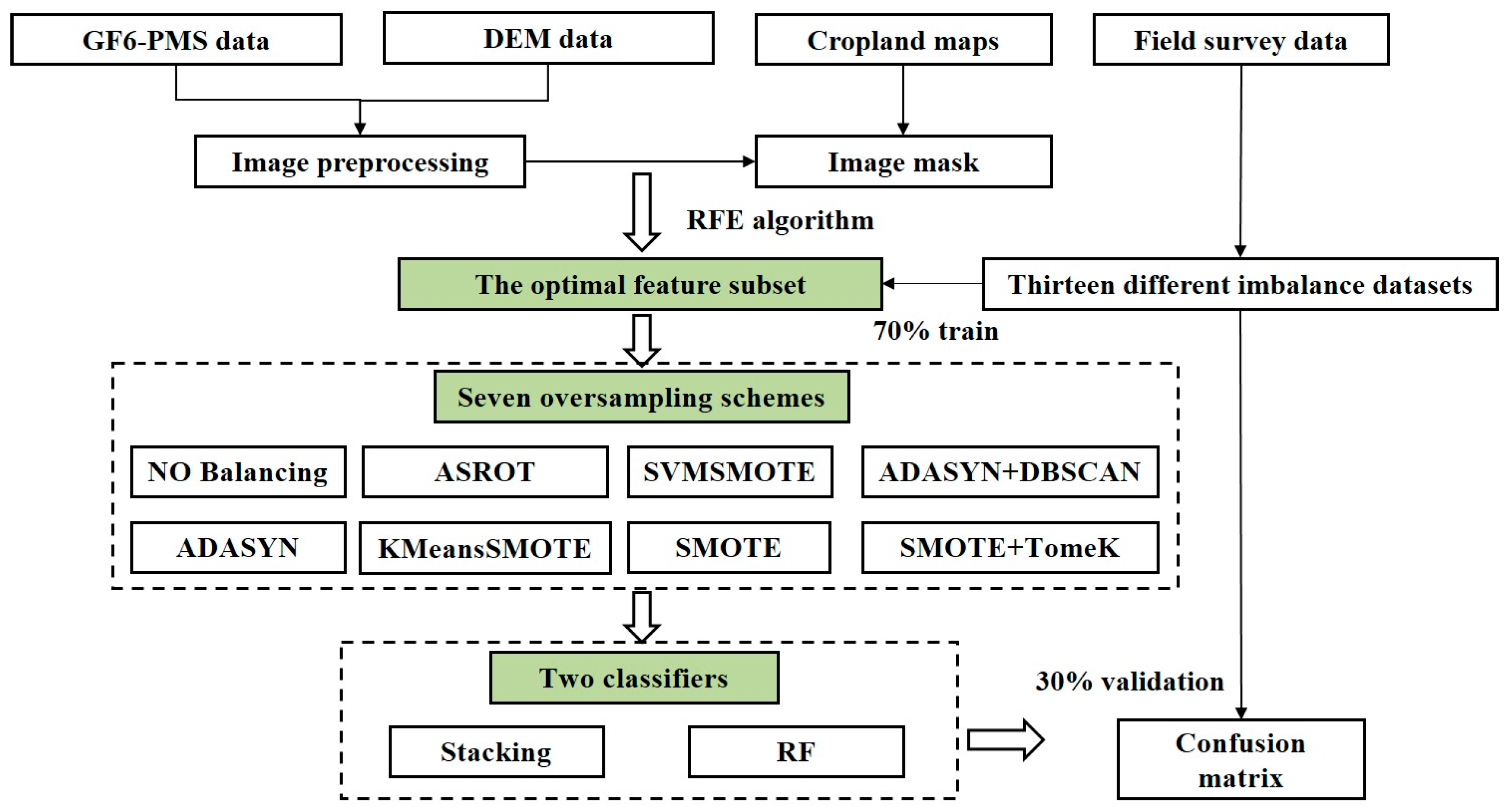
An overview of the workflow is shown in Figure 2. First, the GF-6 images were pre-processed, and then masked using the cropland boundary vector file to extract the farmland areas. Second, the spectral, texture, vegetation index, and terrain features were generated. The recursive feature elimination (RFE) algorithm, which progressively eliminates features based on their relative redundancy, was used to generate a subset of features for use as input variables for the classifiers. A total of 13 imbalanced training datasets encompassing different crop classes and sample sizes were generated from ground survey data and associated ROIs. These training datasets were preprocessed by various rebalancing schemes, and then used as inputs of two classifiers for crop classification. These steps are explained in more detail below.

3.1. Feature Space Creation

In our previous study [10], we identified ten optimal variables for crop classification in this complex and high-elevation agricultural landscape, by using the 70% samples of dataset 13 (Figure 3a). Here, the frequency of these samples does represent that of the entire dataset 13, with benefit from the scikit-learn Python package (with random seed set as zero) for 7:3 randomly train–test-split process. The variables were selected using random forest classification (RF) combined with recursive feature elimination (RFE) [40,41], i.e., a RF-RFE strategy, and were found to support a high overall accuracy of 97.71% (Figure 3b).
The ten optimal variables include three spectral bands, two vegetation indices, four texture features and a single topographic feature (Table 3). The spectral bands green, red, and NIR comprise three of the original four GF-6 bands. The two indices, i.e., the triangular vegetation index (TVI) and the green normalized difference vegetation index (GNDVI), are both sensitive to the green peak of canopy spectra. TVI is also sensitive to the absorption of radiative energy by vegetation pigments [42], while GNDVI is sensitive to chlorophyll-a concentration [43]. The texture bands were derived from the gray level co-occurrence matrix (GLCM), with a 3 × 3 processing window, one pixel co-occurrence shift, and a 64-greyscale quantization [44]. The GLCM mean operator is a type of smoothing function. The last feature selected, elevation, was the 10 m DEM data, resampled to a 2 m pixel size using cubic convolution, for conformity with the GF-6 images. This feature is important for crop classification accuracy because elevation affects local climate and thus crop growth [45].

3.2. Resampling Algorithms

To improve the classification of minor crop types in high-elevation regions, we proposed a new resampling algorithm, Adaptive synthetic and repeat oversampling technique, ASROT based on the ADASYN and DBSCAN algorithms [27,32], to generate balanced training datasets for driving the classification of crops, especially the minor crops that typically occupy few areas within a scene. Here, the proposed ASROT algorithm was also compared with five existing resampling algorithms. The details of each algorithm are discussed in the following sections.

3.2.1. Adaptive Synthetic Sampling (ADASYN)

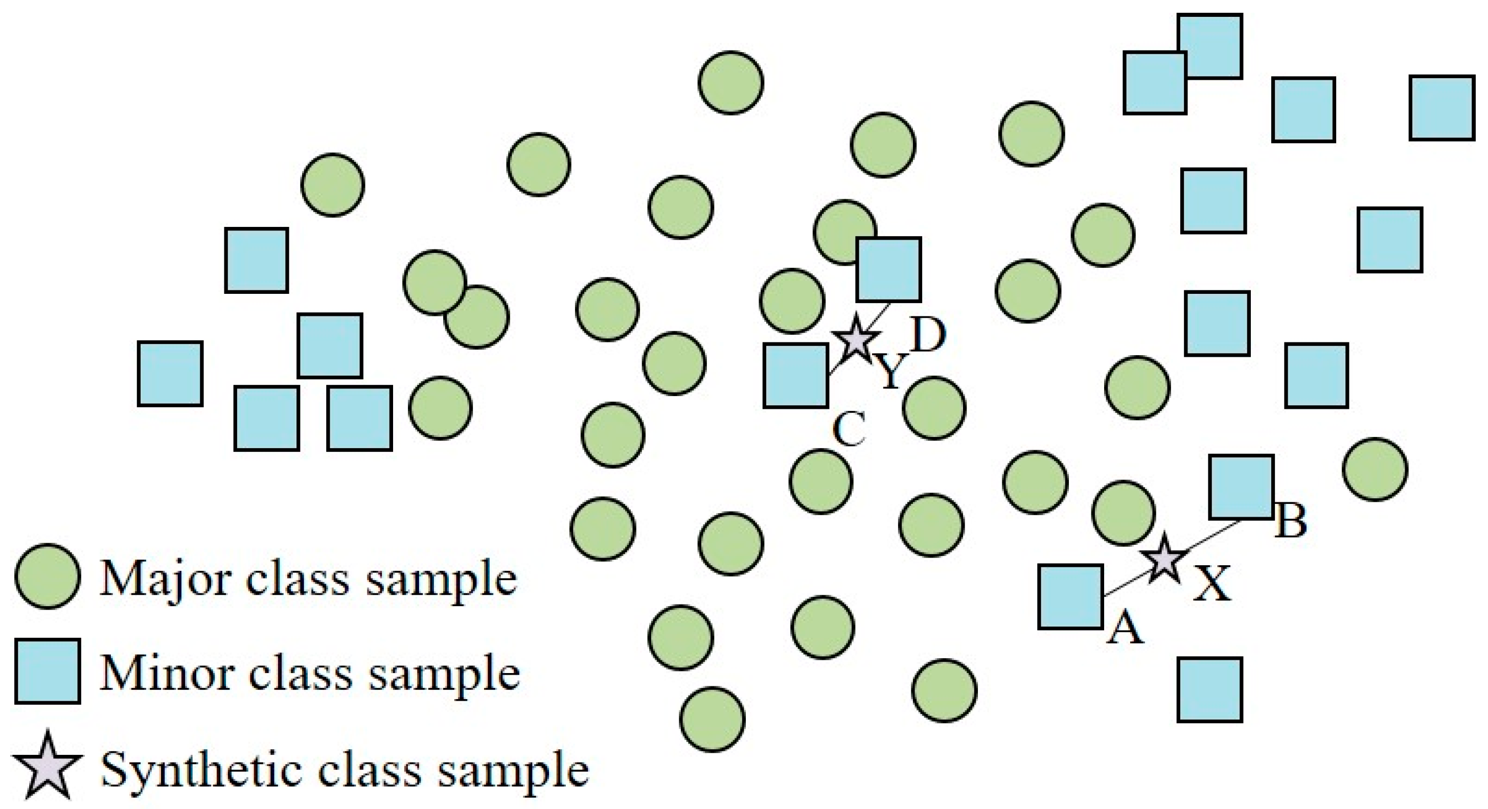
The ADASYN algorithm improves upon the SMOTE algorithm by adaptively determining the number of samples to generate for each minority category [27]. Specifically, the number of interpolated synthetic samples is increased for existing minority class samples that are regarded as the most difficult to learn. The minority class is defined for those samples with the greatest proportion of their K nearest neighbors belonging to a different class. This has the effect of increasing the proportion of minority class samples in the feature space at the boundaries of the distribution of that class, and for small, isolated groups of minority samples. As shown in Figure 4, the ADASYN algorithm synthesizes new samples between samples A and B by linear interpolation, to add the minority-class samples that are close to the majority class. This can improve the classification performance of the model [46]. However, unlike the points A and B in Figure 4, the points C and D may be noisy points and the synthesized sample Y may mislead the classification model. Therefore, it is desirable to eliminate potential noise samples (e.g., the synthetic minor-crop samples with similar spectral reflectance to major crop) as much as possible after using the ADASYN algorithm, and thus improve the classification accuracy. In this study, the ADASYN algorithm was run by using imbalanced-learn Python package with its hyperparameters set as default, except the sampling strategy and random state. The former was set as all, while the later was set as zero.

3.2.2. Density Based Spatial Clustering of Applications with Noise (DBSCAN)

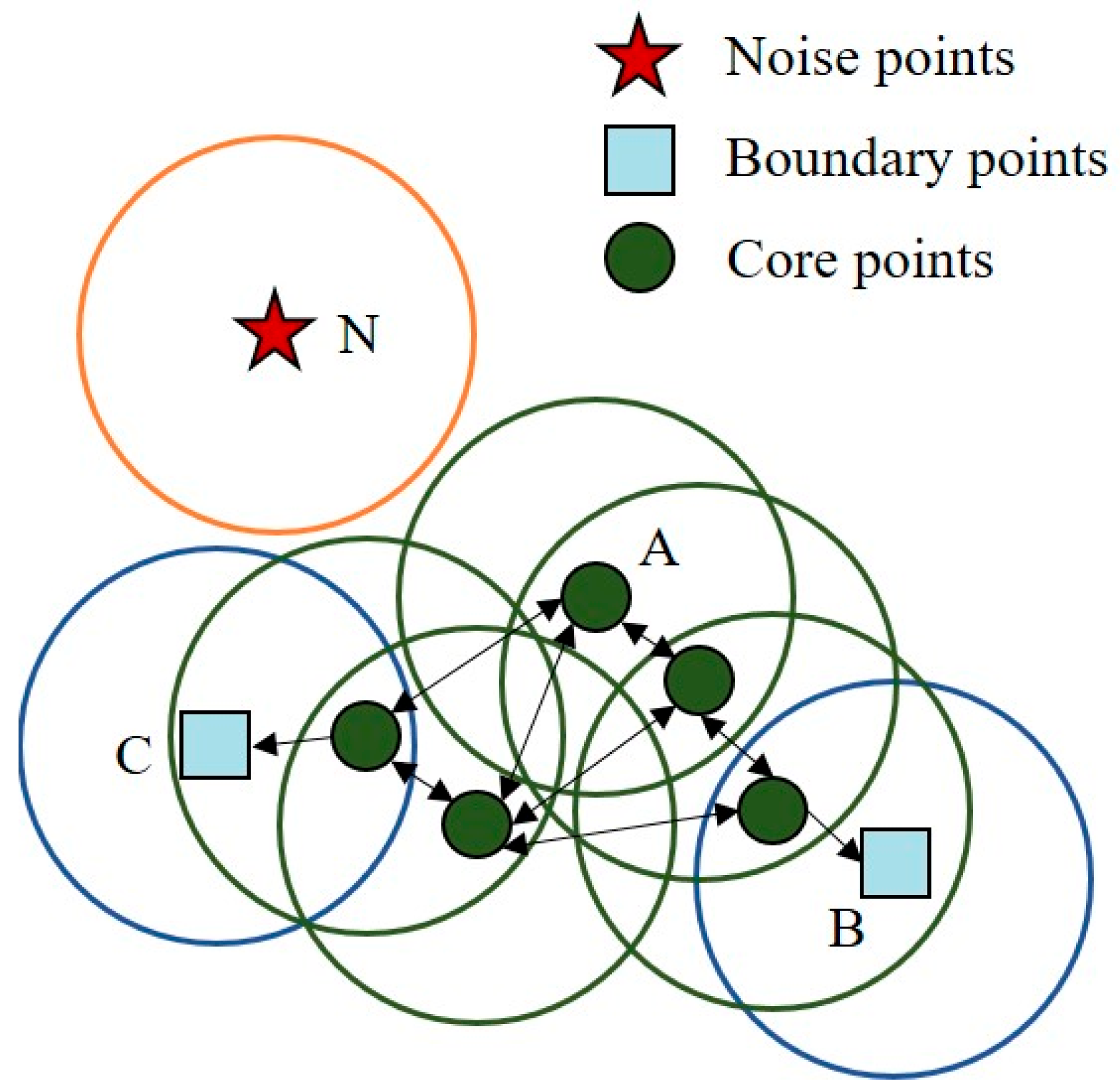
DBSCAN is a clustering algorithm that distinguishes between high- and low-density regions in the feature space [32,47,48]. The working principle of the DBSCAN algorithm is shown in Figure 5. DBSCAN uses only two parameters: the radius (eps) that defines the circular search region around each sample in the feature space, and the minimum number of samples (mpt) within that search region to be regarded as a core high-density region. All samples belong to one of three classes: core, border, or noise. Core samples are those with more than mpts samples within their search region. In Figure 5, the samples shown in green are core samples for an mpt value of two. The samples B and C are both classified as boundary samples, since they have less than mpt samples within the circle centered on those samples, but nevertheless are within the radius of circles centered on core samples. Noise samples, such as N, have less than mpt samples with their circles, and do not fall within the radius of core samples. The DBSCAN algorithm, shown to identify isolated samples, is a useful way of classifying noise [49]. It has great potential to detect outliers in the training data. In this study, the DBSCAN algorithm was run using the scikit-learn Python package with its parameters set to default.

3.2.3. Adaptive Synthetic and Repeat Oversampling Technique (ASROT)

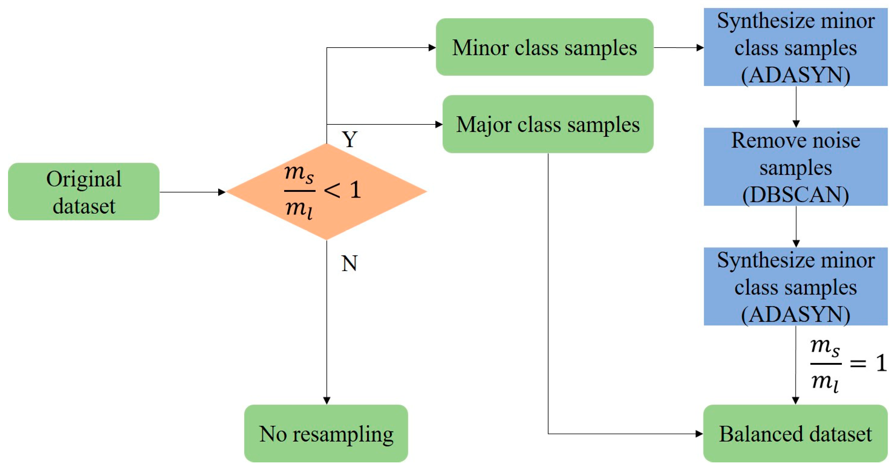
In this study, we combined ADASYN and DBSCAN algorithms to propose a new resampling algorithm (ASROT) for generating high-quality oversampled training datasets. The workflow of the ASROT algorithm is shown in Figure 6. Due to the small sample size of minority classes, the ADASYN algorithm is firstly applied to oversampling the imbalanced dataset, which may result in noise that affects the classification performance. Therefore, the DBSCAN algorithm is applied in the next stage to detect and remove the noise samples, so that the pure samples can be obtained. Finally, the ADASYN algorithm is applied once again to increase the sample size and further balance the datasets.

3.2.4. Other Resampling Algorithms

To evaluate the proposed ASROT algorithm, we firstly set ablation studies with comparison about original ADASYN and ADASYN+DBSCAN algorithms. Meanwhile, we also adopted the SMOTE algorithm and its three classical SMOTE variants for comparison to ASROT. All the SMOTE-related algorithms were run by using the imbalanced-learn Python package. The random seed was set to zero, while the other hyperparameters were set to default. The details of these algorithms are as described below.
SMOTE [20]: This is a classic algorithm to expand the samples of minority class to balance the class distribution of training datasets. This algorithm has been widely used for the cases with imbalanced datasets [23,50]. However, the random selection of target samples in the SMOTE algorithm may fails to account for the distribution of minority classes [51] and may reinforce overlap in the distributions of the classes in the feature space [52].
SVMSMOTE [53]: This method is an oversampling algorithm that synthesizes sample points that lie near the boundary line between the samples from the majority and minority classes. The SVM algorithm is used to identify the hyperplane between classes and the associated support vectors. Synthetic points for the minority class support vectors are then generated using either interpolation between two neighbors, as with SMOTE, or extrapolation (i.e., projection in the opposite direction of the interpolation line, towards the majority class), depending on which class dominates the nearest neighbors of each minority point. If the minority class dominates, extrapolation is used, and if the majority class dominates, interpolation is used. This rule is designed to move the decision boundary between the two classes towards the majority class if the density of the majority class is low in that part of the feature space.
KMeansSMOTE [25]: This method is an oversampling algorithm that synthesizes new points for the minority class in regions of the feature space where the minority class dominates but has low density. First, all samples, irrespective of their class label, are clustered into K clusters using the KMeans algorithm. The number of majority and minority points in each cluster is summed, and only clusters dominated by the minority class are selected for synthesis of new points. New points are synthesized using the SMOTE algorithm, but with the modification that the proportion of new points generated in each cluster is inversely related to the relative density of the cluster. This bias towards generating more points in the low-density clusters is designed to reduce within-class imbalance in the density of the rare class in the feature space. The choice of only using clusters that are dominated by the minority class for synthesizing new points is designed to exclude minority points that cluster with the majority class and that are assumed to represent potential noise in the data.
SMOTE+Tomek links [54]: This method is widely used for under-sampling cases or data cleaning. Pairs of instances that are nearest neighbors to each other, but belong to different classes, are identified by calculating the Euclidean distance between samples. The balance of the data samples is increased by removing sample points from closely adjacent points belonging to the majority class.

3.3. Classification Models

In this study, stacking and RF models were trained based on the imbalanced and balanced datasets. RF is an ensemble of decision trees generated using bootstrapped samples from the training dataset [55]. It can resolve the co-linear issues when dealing with high dimensional datasets and can assess the variable importance for feature selection. Nowadays, RF is widely used for the classification of various crop types based on remote sensing imagery [52,56,57]. In comparison, stacking is also an ensemble learning technique that combines multiple classification models via a meta-learner [58]. It can aggregate multiple typical classifiers and make full use of their advantages [59]. To identify the crop types in high-elevation regions, where fields tend to be small and heterogeneous in shape, our stacking algorithm employs three traditional classification methods for crop classification, RF, XGBoost, and AdaBoost, as reported in our previous study [10]. For each dataset, we trained the classification models based on a random 70% subset of samples and validated the models on the remaining 30% of the samples. All above processes were conducted by using scikit-learn and xgboost Python packages, with hyperparameters and random seed set to default and zero, respectively.

3.4. Accuracy Assessment and Statistical Analysis

For the accuracy assessment, we used the class-based metrics of user’s accuracy (UA), producer’s accuracy (PA), and F1-score, which are calculated from the confusion matrix [60]. In addition, overall accuracy (OA), which represents the proportion of pixels that are correctly classified, was used as a summary accuracy metric. Since OA, by definition, is weighted according to the proportions of each class, we also calculated the macro F1-score of all classes for each dataset [61]. The formula is as the following:
M a c r o   F 1 s c o r e = i = 1 j F 1 i / j
where F 1 i is the F1-score of the class i and j is the number of classes.
In addition, we used a combination of the Friedman test and the post hoc Nemenyi test to evaluate the difference between the classification accuracy of the newly proposed ASROT algorithm and the traditional resampling algorithms. The Friedman test is a nonparametric multiple comparison test using rank to evaluate whether there is a significant difference between three or more variables, in this case accuracies [62]. If the Friedman test indicates a rejection of the null hypothesis that there is no significant difference in the accuracies, the Nemenyi follow-up test is applied to determine which accuracies are significantly different.

3.5. Application of ASROT Algorithm for Crop Mapping

Then, the ASROT was applied to the measured dataset, i.e., the dataset 13 of Table 2, to obtained balanced one. Both the datasets before and after using ASROT algorithm were used to drive the classification of crop types, so that we can test the contribution of ASROT algorithm to the classification accuracy of various crop types. Here, like the Section 3.3, the classification models were trained based on a random 70% subset of samples and validated by using the remaining 30% of the samples. In addition, the obtained models were further used for crop mapping at the regions encompassing two minor crops (i.e., broad beans and highland barley). Therefore, we could compare the crop maps before and after using ASROT algorithm.

4. Results

4.1. Effect of Imbalanced Dataset on Classification Performance

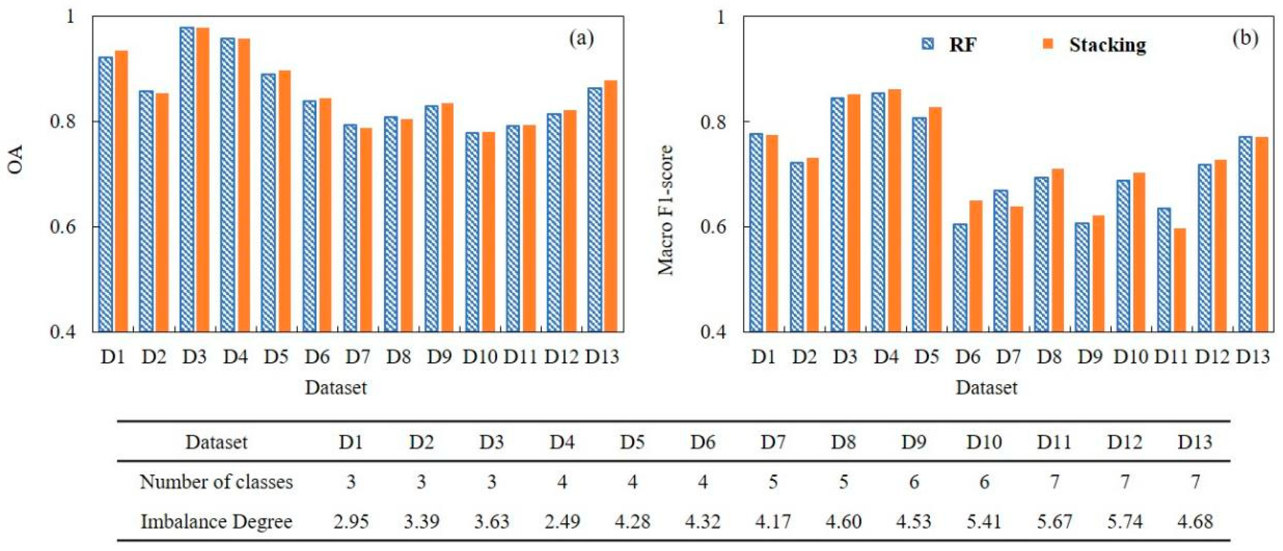
Figure 7 summarizes the accuracy results of the thirteen datasets prior to balancing the class proportions in the training data. The OA values of the RF model range from 77% to 95%, and those of the stacking model range between 78% and 98% (Figure 7a). Among the thirteen datasets, dataset No. 3 (D3), i.e., the Rapev–HBl–BBl dataset, produces the highest OA values, while dataset No. 10 (D10), the Wheati–Rapeh–Maizei–Potatoh–BBi–OCi dataset, has the lowest OAs. In the groups with all classes (i.e., D11, D12, and D13), the datasets of low imbalance degree tend to produce higher accuracy than that of high imbalance degree. However, this relationship is varied where datasets encompass the small number of classes and the difference of crop types, because the algorithm-level response to crop types is different.
Figure 7b shows the RF and stacking classifiers respectively achieve macro F1-score values that range from 55% to 86% and from 42% to 86%, respectively. Among the thirteen datasets, D4, i.e., the Wheath–Rapel–Potatol–HBl dataset, produces the highest macro F1-score value. D11, i.e., the Wheatv–Rapeh–Maizei–Potatoi–HBl–BBl–OC dataset, has the lowest macro F1-score value. In comparison to the RF model, the stacking model generally produces slightly higher OA and macro F1-score values, with the notable exceptions of D7 and D11.
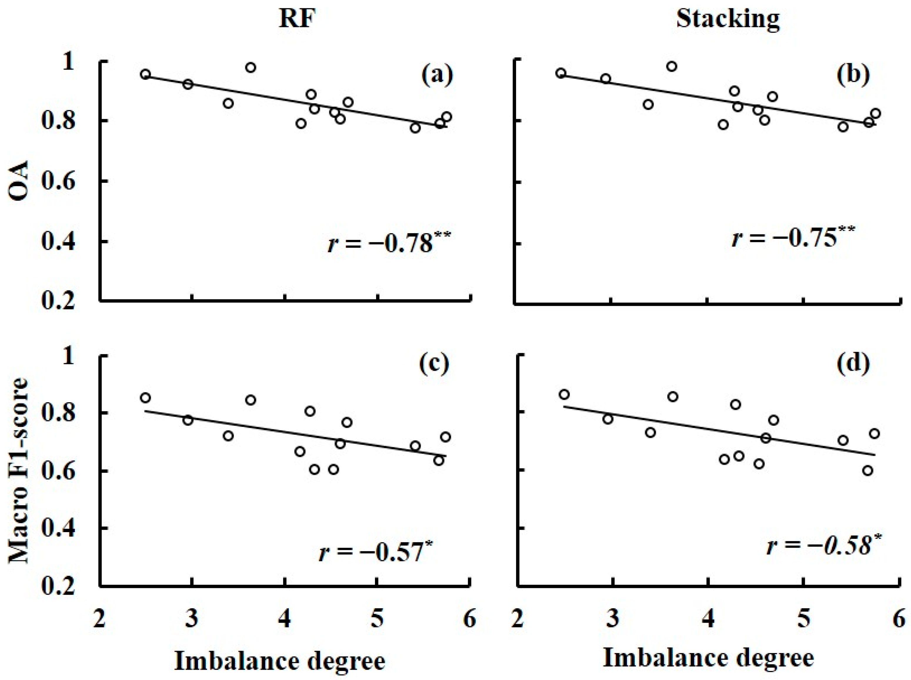
Figure 8a,b show a significant and negative correlation between OA value and imbalance degree, with r = −0.78 and r = −0.75 for RF and stacking models, respectively. Similarly, there is a negative correlation between macro F1-score and imbalance degree, with −0.57 and −0.58 for RF and stacking models, respectively (Figure 8c,d). These results confirm that higher imbalance values are associated with lower accuracy.

4.2. Comparison of Classification Accuracies of the Different Resampling Algorithms

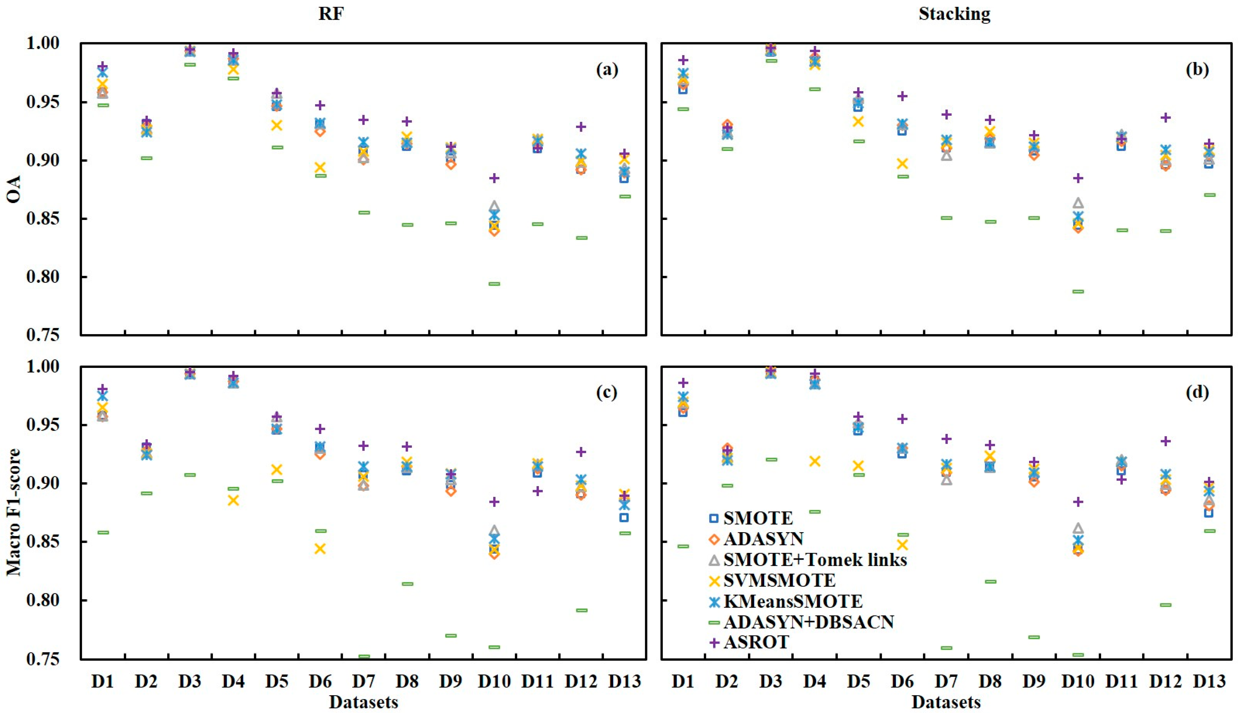
Figure 9 graphs OA and macro F1-score after the application of the seven resampling algorithms, including SMOTE, ADASYN, SMOTE+Tomek links, SVMSMOTE, KMeansSMOTE, ADASYN+DBSCAN, and ASROT algorithms. The balanced training datasets produce classification accuracy with OA and macro F1-score values over 80% for both the RF and stacking classifiers. Overall, the stacking classifier slightly outperforms the RF classifier, as it does for the imbalanced datasets.
The proposed ASROT algorithm generally outperforms other six algorithms in balancing training datasets for crop classification based on RF or stacking classifiers. D12 (the Wheati–Rapei–Maizeh–Potatoh–HBv–BBv–OCi dataset), with the highest degree of imbalance, illustrates the benefits of balancing the training data. Before balancing, the classification of D12 with the RF model results in OA = 81.48% and macro F1-score = 71.82%, and classification with the stacking model resulted in OA = 82.22% and macro F1-score = 73.54% (Figure 7). After balancing the training dataset by ASROT algorithm, the subsequent classification accuracy is OA = 92.87% and macro F1-score = 92.70% for the RF classifier, and OA = 93.69% and macro F1-score = 93.62% for the stacking classifier (Figure 9).
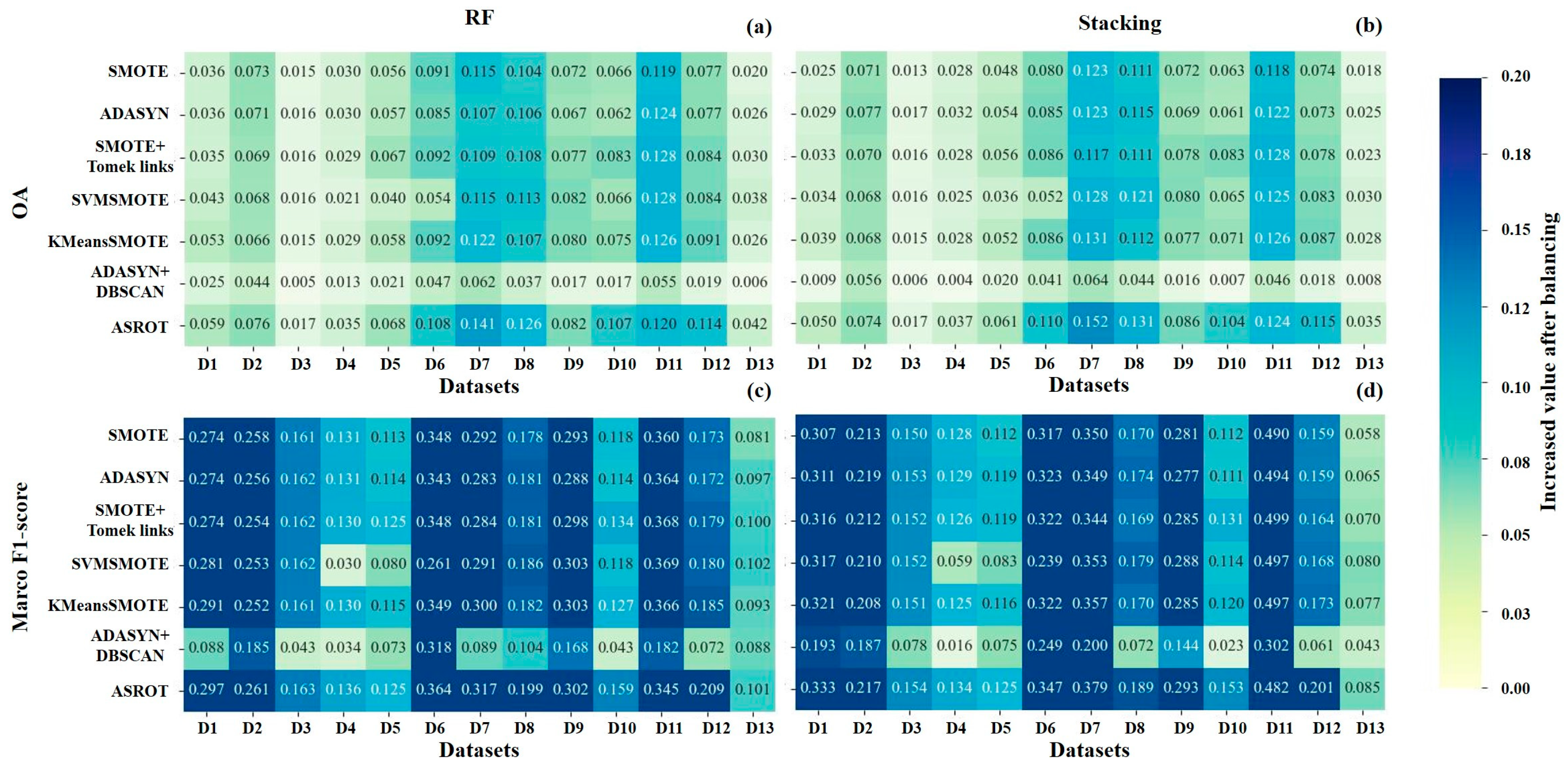
After balancing, all six resampling algorithms show an increase in OA and macro F1-score for both RF and stacking model classifications (Figure 10). Training datasets with large imbalance generally result in greater improvements in accuracy. For instance, the six resampling algorithms increase the classification accuracy of D7, the Wheati–Rapei–Potatol–BBl–OCh dataset, by raising the OA values by 10.7% to 14.1% for the RF classifier, and 11.7% to 15.2% for the stacking classifier (Figure 10a,b). Similarly, the corresponding macro F1-score values following balancing increase from 28.3% to 31.7% and from 34.4% to 37.9% for the RF and stacking classifiers, respectively (Figure 10c,d). Overall, the proposed ASROT provides the greatest increase in accuracy for most datasets, and thus appears to be the most effective balancing method, at least for these datasets.
The Friedman and Nemenyi follow-up tests were applied to evaluate the statistical significance of the differences in the accuracies of the seven resampling algorithms (Figure 11). The results show that the ranking of seven different resampling algorithms for RF classifier (Figure 11a) is broadly like that for stacking classifier (Figure 11b). Although the ADAYSN algorithm is assigned slightly different ranks for RF and stacking classifier accuracies, the proposed ASROT algorithm consistently has the highest average rank, outperforming other six resampling algorithms. In contrast, the ADAYSN+DBSCAN approach is consistently ranked last, with relatively poor performance in balancing training datasets.

4.3. Improvements in Classification Accuracy Following Application of the ASROT Algorithm

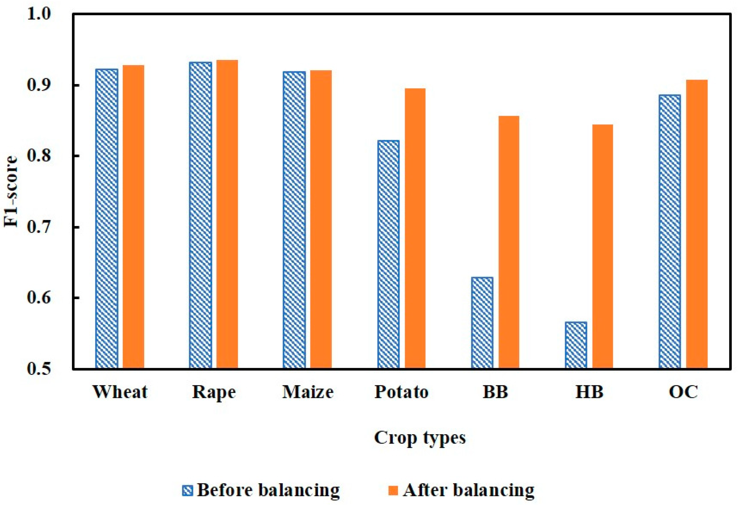
Because the stacking classifier generally outperforms RF classifier according to above results, the former was further used to test the performance of ASROT algorithm in dealing with imbalance samples. Table 4 shows the classification accuracy (UA, PA, and F1-score) of crop types before and after using the ASROT resampling algorithm and based on the original training dataset with 186,381 samples (i.e., dataset 13 in Table 2). The results show that the proposed ASROT algorithm could balance the training datasets and improve the classification accuracy of all crop types. Particularly, this algorithm improves the classification of minor crops including broad beans and highland barley, both of which have a sample size much smaller than those of the major crops. The classification accuracy of highland barley increases from UA = 50.41%, PA = 64.58%, and F1-score = 56.62% to UA = 83.99%, PA = 84.65%, and F1-score = 84.32%, while the classification accuracy of broad beans improves to UA = 87.02%, PA = 84.32%, and F1-score = 85.65%. In summary, the ASROT algorithm results in small to moderate increases in accuracy of the major crops, and the accuracy of the minor crops rises by approximately 30%.
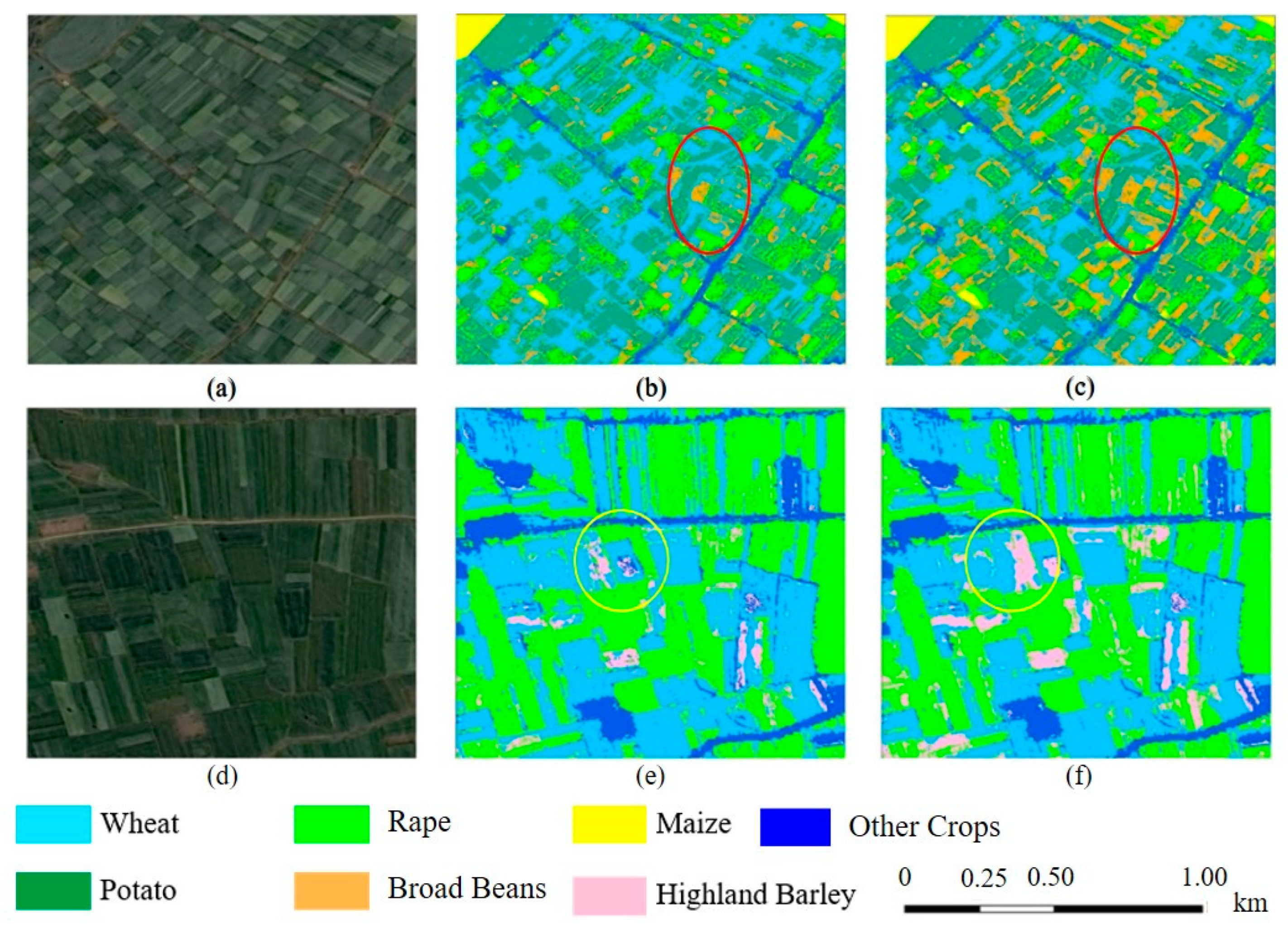
For testing ASROT algorithm in classification of minor crops, two areas of 600 by 600 pixels were extracted from GF6 images, in which the two minor crops of broad beans and highland barley were found. In the first area, wheat, rape, potato, and broad beans predominated (Figure 12a), while in the second area wheat, rape, and highland barley were most common (Figure 12d). In this region, the crop fields are small, causing high spatial heterogeneity. The stacking model classification using the original dataset results in confusion in the labeling of both broad beans and highland barley (Figure 12b,e). In contrast, after applying the ASROT algorithm, the stacking model produces a more homogenous classification of broad beans and highland barley (Figure 12c,f). For example, in the classification using the original data, the center of the highland barley fields tends to be misclassified as other vegetation types (Figure 12e), whereas the classification after ASROT balancing reduces this problem (Figure 12f).

5. Discussion

5.1. Effect of Sample Imbalance on the ML-Based Crop Classification

The balance of training samples plays a key role in determining the accuracy of crop classification using ML algorithms. The larger the imbalance, the lower the accuracy of the crop classification, particularly for the classes with fewer training samples [63]. In general, for agricultural scenes, imbalanced training datasets occur when the minor crops of complex cropping structures cover only small areas on the ground, allowing only limited numbers of training samples for those crops [64]. Imbalance in the training datasets is a common problem for crop classification base on satellite images [4,65,66]. Improving the classification accuracy of minor crops is closely dependent on reducing the imbalance of training dataset (Figure 12), without reducing the overall number of samples. In the future, balancing training datasets before using them to drive ML classification of crops, especially the minor crops, should be a common pre-processing step.

5.2. Importance of the Choice Resampling Algorithm for Crop Classification of Complex Scenes

The combination of resampling and noise-detection algorithms is an effective approach for balancing training samples for crop classification. As reported by a previous study [67], traditional resampling algorithms, such as the SMOTE algorithm, typically produce additional noise samples in the resulting training datasets. These additional noise samples have a deleterious effect on crop classification, reducing the benefits of synthesizing additional training data. Thus, a common approach for balancing training samples is to combine SMOTE and outlier-detection algorithms [30,68,69]. However, the performance of such an approach has not been previously evaluated in the context of crop classification applied to complex agriculture systems. In this study, the previously developed ADASYN and DBSCAN algorithms were combined to generate the novel ASROT approach. In the experiments undertaken in this study, ASROT outperformed existing resampling algorithms in balancing training datasets for crop classification in high-elevation regions (Figure 11). It produced the highest OA for most of our synthetic datasets (Figure 9), illustrating the effectiveness of ASROT balancing of the training data for crop classification of complex agriculture systems.
Ensemble learning algorithms are particularly dependent on the choice of resampling algorithm. As reported by previous studies [59,70], although most ensemble learning algorithms can potentially produce high accuracies when used in multiclass classification, the resulting classification accuracy is closely dependent on the quality of training datasets, i.e., the balance of class distribution. Our results support these findings, as the classification accuracy of maps derived by both RF and stacking classifiers are generally negatively correlated with the imbalance degree (Figure 8). In practice, the minor crops (particularly broad beans and highland barley) typically have fewer samples in comparison to the major crops, and thus classification accuracy of these rare classes is relatively low (Table 4). Fortunately, resampling algorithms can reduce the negative effect of imbalance in the training data, thus improving the accuracy of crop classification. As our experiments have shown (Figure 9), application of the ASROT algorithm to dataset D12 (the Wheati–Rapei–Maizeh–Potatoh–HBv–BBv–OCi dataset), which has a high imbalance degree, improves OA of the RF and stacking models by over 10% after the balancing process. Furthermore, even the somewhat more balanced dataset 13 (the original training dataset), which has the largest number of samples for training samples of all our experiments, shows evidence of improved classification accuracy after applying the ASROT algorithm (Figure 12). Moreover, the good classification accuracy partly demonstrates the generalization of ensemble learning algorithms, because the training samples were derived from eight cloud-free images across three strips (Section 2.2). Generally, sample balance algorithms (e.g., ASROT) do improve the accuracy of data-driven approach, e.g., RF and stacking algorithms, but remaining unclear about the generalization of crop classification models across other regions. Further effort needs to explore the generalization of crop classification models at algorithm level.

5.3. Potential of ASROT Algorithm to Improve Classification Accuracy of Minor Crops

Most cropping systems typically encompass both major and minor crops. Although minor crops occupy only a small percentage of crop areas, they still play an important role in increasing crop diversity and promoting sustainable development [71]. However, the collection of training samples is limited by the few areas with minor crops present, causing the problem about the imbalance of class distribution. This issue makes it difficult to map the distribution of minor crops accurately using remote sensing images [72]. In this study, the ASROT algorithm is proposed to reduce noise in synthesizing new class samples, and thus improves the classification accuracy of minor crops. In our experiments, after using the ASROT algorithm to balance the training dataset, the classification accuracy of minor crops is greatly improved, resulting in an F1-score value over 0.8 for all crop types (Figure 13). A notable feature is that the ASROT-balanced training dataset also tended to slightly increase the classification accuracy of major crops compared to the original datasets.
As a special crop in high-altitude regions, highland barley is a typical minor crop within the study area. Due to topographic constraints (highland barley is often planted at 2500–4500 m above sea level), climate factors (e.g., temperature and light), and human factors, highland barley is usually only a minor crop in highland agricultural systems. Because of comparatively few available training areas, highland barley is generally mapped with low accuracy using remote sensing [73]. Adding predictor variables, especially DEM data, can only somewhat mitigate this problem [10]. Indeed, increasing the number of predictor variables generally increases the importance of employing a sufficiently large training dataset, a problem known as the curse of dimensionality or the Hughes phenomenon [74,75]. In this study, the proposed ASROT algorithm enhances the feature information used to distinguish minor crops by expanding the sample size of highland barley and broad beans (Table 4). Benefitting from the noise removal for high-quality training data, the ASROT algorithm has broad application in the classification of crops, especially in complex agriculture systems with minor crops.

5.4. Effect of Interaction Between the Spectral Distortion and Texture Features of Panchromatic Fusion

The panchromatic fusion can contribute to the classification accuracy of crop types at altitude regions. In previous, substantial studies used panchromatic fusion to enhance the spatial resolution of satellite images with dependence on the panchromatic bands [76,77]. This fusion process can improve image texture, but the spectral distortion certainly occurs [78]. The trade-off between them affects the final classification accuracy. For the regions with high heterogeneity, this trade-off tends to improve the classification accuracy of crop types. As mentioned by a recent study [79], the regions with various land covers encompass high spatial heterogeneity, while the NNDiffuse algorithm is superior in Pan sharpening and does improve the classification accuracy of land cover, even if the spectral distortion occurs. Similarly, due to the complex terrain (Figure 1), the crop classification in high-altitude areas is particularly dependent on the images with fine resolution. So, this study adopted the NNDiffuse algorithm to produce the synthetic images with fine resolution (Section 2.2). With benefit from the low spatial heterogeneity of every pixel, the obtained model can produce good classification accuracy for various crop types (Table 4). In future, effort is worthy to improve panchromatic fusion algorithms, so that the obtained synthetic images can encompass both good spectral and texture information for observing land covers.

6. Conclusions

This study aimed to improve crop classification in complex agricultural systems that have both major and minor crops. To address the problem of imbalanced training datasets, the ASROT resampling algorithm that combines the existing ADASYN and DBSCAN algorithms was proposed. In our experiments, we generated 13 imbalanced datasets, which were used as training data for the RF and stacking models in crop classifications. These classifications confirmed that imbalance reduces the crop classification accuracy. The correlation between the imbalance degree of the training data and OA is negative, with r = −0.78 for RF and r = −0.75 for stacking models. After applying the proposed ASROT resampling algorithm and six other previously developed algorithms to balance training datasets, the accuracy of the model was improved, especially for minor crops, with small training sample sizes. The ASROT algorithm outperformed the other resampling algorithms tested. It is robust across multiple training datasets, comprising a range of classes, training sample sizes, and imbalance degree levels. The stacking model trained with data balanced with the ASROT algorithm results in greatly improved classification accuracy of minor crops, without a reduction in the accuracy of the classification of the major crops. For example, after balancing, the classification accuracy of minor crops is F1 = 85.65% for broad beans and F1 = 84.32% for highland barley, compared to 62.86% and 56.62%, respectively prior to rebalancing. Further research is needed to investigate the application of the ASROT resampling algorithm to balance training datasets of other complex agricultural systems.

Author Contributions

Conceptualization, W.L., Z.M. and X.Y.; Methodology, J.Z. and Z.M.; Software, J.Z.; Formal analysis, W.L.; Investigation, T.L.; Resources, C.J., Y.T. and X.Y.; Data curation, W.L., J.Z., T.L. and H.Z.; Writing—original draft, W.L. and X.Y.; Writing—review & editing, W.L., J.Z., Z.M., T.A.W., H.Z., C.J., T.C., Y.T., Y.Z., W.C. and X.Y.; Supervision, T.C., W.C. and X.Y.; Funding acquisition, Y.Z., W.C. and X.Y. All authors have read and agreed to the published version of the manuscript.

Funding

This work was supported by the National Key Research and Development Program of China (2022YFD2001104), Fundamental Research Funds for the Central Universities (XUEKEN2022018, KYPT2024009, CXCYL2024003), National Natural Science Foundation of China (32471996), Jiangsu Province “333 High-level Talents Training Project”, Jiangsu Collaborative Innovation Center for Modern Crop Production (JCICMCP), National Postdoctoral Program for Innovative Talents (BX20250023), Jiangsu Funding Program for Excellent Postdoctoral Talent. We thank the anonymous reviewers who provided helpful comments for the manuscript improvement.

Data Availability Statement

The raw data supporting the conclusions of this article will be made available by the authors on request.

Conflicts of Interest

The authors declare no conflict of interest.

References

  1. Fritz, S.; See, L.; Bayas, J.C.L.; Waldner, F.; Jacques, D.; Becker-Reshef, I.; Whitcraft, A.; Baruth, B.; Bonifacio, R.; Crutchfield, J. A comparison of global agricultural monitoring systems and current gaps. Agric. Syst. 2019, 168, 258–272. [Google Scholar] [CrossRef]
  2. Lobell, D.B.; Thau, D.; Seifert, C.; Engle, E.; Little, B. A scalable satellite-based crop yield mapper. Remote Sens. Environ. 2015, 164, 324–333. [Google Scholar] [CrossRef]
  3. Vanino, S.; Nino, P.; De Michele, C.; Bolognesi, S.F.; D’Urso, G.; Di Bene, C.; Pennelli, B.; Vuolo, F.; Farina, R.; Pulighe, G. Capability of Sentinel-2 data for estimating maximum evapotranspiration and irrigation requirements for tomato crop in Central Italy. Remote Sens. Environ. 2018, 215, 452–470. [Google Scholar] [CrossRef]
  4. Waldner, F.; Chen, Y.; Lawes, R.; Hochman, Z. Needle in a haystack: Mapping rare and infrequent crops using satellite imagery and data balancing methods. Remote Sens. Environ. 2019, 233, 111375. [Google Scholar] [CrossRef]
  5. Cai, J.; Luo, J.; Wang, S.; Yang, S. Feature selection in machine learning: A new perspective. Neurocomputing 2018, 300, 70–79. [Google Scholar] [CrossRef]
  6. Lu, D.; Weng, Q. A survey of image classification methods and techniques for improving classification performance. Int. J. Remote Sens. 2007, 28, 823–870. [Google Scholar] [CrossRef]
  7. Ramezan, C.A.; Warner, T.A.; Maxwell, A.E.; Price, B.S. Effects of training set size on supervised machine-learning land-cover classification of large-area high-resolution remotely sensed data. Remote Sens. 2021, 13, 368. [Google Scholar] [CrossRef]
  8. Xiao, Y.; Huang, J.; Weng, W.; Huang, R.; Shao, Q.; Zhou, C.; Li, S. Class imbalance: A crucial factor affecting the performance of tea plantations mapping by machine learning. Int. J. Appl. Earth Obs. Geoinf. 2024, 129, 103849. [Google Scholar] [CrossRef]
  9. Foody, G.M.; Mathur, A. The use of small training sets containing mixed pixels for accurate hard image classification: Training on mixed spectral responses for classification by a SVM. Remote Sens. Environ. 2006, 103, 179–189. [Google Scholar] [CrossRef]
  10. Ma, Z.; Li, W.; Warner, T.A.; He, C.; Wang, X.; Zhang, Y.; Guo, C.; Cheng, T.; Zhu, Y.; Cao, W. A framework combined stacking ensemble algorithm to classify crop in complex agricultural landscape of high altitude regions with Gaofen-6 imagery and elevation data. Int. J. Appl. Earth Obs. Geoinf. 2023, 122, 103386. [Google Scholar] [CrossRef]
  11. Khoury, C.K.; Bjorkman, A.D.; Dempewolf, H.; Ramirez-Villegas, J.; Guarino, L.; Jarvis, A.; Rieseberg, L.H.; Struik, P.C. Increasing homogeneity in global food supplies and the implications for food security. Proc. Natl. Acad. Sci. USA 2014, 111, 4001–4006. [Google Scholar] [CrossRef]
  12. Prati, R.C.; Batista, G.E.; Silva, D.F. Class imbalance revisited: A new experimental setup to assess the performance of treatment methods. Knowl. Inf. Syst. 2015, 45, 247–270. [Google Scholar] [CrossRef]
  13. Johnson, J.M.; Khoshgoftaar, T.M. Survey on deep learning with class imbalance. J. Big Data 2019, 6, 27. [Google Scholar] [CrossRef]
  14. LemaÃŽtre, G.; Nogueira, F.; Aridas, C.K. Imbalanced-learn: A python toolbox to tackle the curse of imbalanced datasets in machine learning. J. Mach. Learn. Res. 2017, 18, 1–5. [Google Scholar]
  15. He, H.; Garcia, E.A. Learning from imbalanced data. IEEE Trans. Knowl. Data Eng. 2009, 21, 1263–1284. [Google Scholar] [CrossRef]
  16. Cheng, R.; Zhang, L.; Wu, S.; Xu, S.; Gao, S.; Yu, H. Probability density machine: A new solution of class imbalance learning. Sci. Program. 2021, 2021, 7555587. [Google Scholar] [CrossRef]
  17. Liu, J. Importance-SMOTE: A synthetic minority oversampling method for noisy imbalanced data. Soft Comput. 2022, 26, 1141–1163. [Google Scholar] [CrossRef]
  18. Dubey, H.; Pudi, V. Class based weighted k-nearest neighbor over imbalance dataset. In Advances in Knowledge Discovery and Data Mining, Proceedings of the Pacific-Asia Conference on Knowledge Discovery and Data Mining, Gold Coast, Australia, 14–17 April 2013; Springer: Berlin/Heidelberg, Germany, 2013; pp. 305–316. [Google Scholar]
  19. Elreedy, D.; Atiya, A.F. A comprehensive analysis of synthetic minority oversampling technique (SMOTE) for handling class imbalance. Inf. Sci. 2019, 505, 32–64. [Google Scholar] [CrossRef]
  20. Chawla, N.V.; Bowyer, K.W.; Hall, L.O.; Kegelmeyer, W.P. SMOTE: Synthetic minority over-sampling technique. J. Artif. Intell. Res. 2002, 16, 321–357. [Google Scholar] [CrossRef]
  21. Ebrahimy, H.; Mirbagheri, B.; Matkan, A.A.; Azadbakht, M. Effectiveness of the integration of data balancing techniques and tree-based ensemble machine learning algorithms for spatially-explicit land cover accuracy prediction. Remote Sens. Appl. Soc. Environ. 2022, 27, 100785. [Google Scholar] [CrossRef]
  22. Han, L.; Yang, G.; Yang, X.; Song, X.; Xu, B.; Li, Z.; Wu, J.; Yang, H.; Wu, J. An explainable XGBoost model improved by SMOTE-ENN technique for maize lodging detection based on multi-source unmanned aerial vehicle images. Comput. Electron. Agric. 2022, 194, 106804. [Google Scholar] [CrossRef]
  23. Fernández, A.; Garcia, S.; Herrera, F.; Chawla, N.V. SMOTE for learning from imbalanced data: Progress and challenges, marking the 15-year anniversary. J. Artif. Intell. Res. 2018, 61, 863–905. [Google Scholar] [CrossRef]
  24. García, V.; Sánchez, J.S.; Mollineda, R.A. Classification of high dimensional and imbalanced hyperspectral imagery data. In Pattern Recognition and Image Analysis, Proceedings of the Iberian Conference on Pattern Recognition and Image Analysis, Las Palmas de Gran Canaria, Spain, 8–10 June 2011; Springer: Berlin/Heidelberg, Germany, 2011; pp. 644–651. [Google Scholar]
  25. Douzas, G.; Bacao, F.; Last, F. Improving imbalanced learning through a heuristic oversampling method based on k-means and SMOTE. Inf. Sci. 2018, 465, 1–20. [Google Scholar] [CrossRef]
  26. Bache, K.; Lichman, M. UCI Machine Learning Repository; School of Information and Computer Science, University of California: Irvine, CA, USA, 2013. [Google Scholar]
  27. He, H.; Bai, Y.; Garcia, E.A.; Li, S. ADASYN: Adaptive synthetic sampling approach for imbalanced learning. In Proceedings of the 2008 IEEE International Joint Conference on Neural Networks (IEEE World Congress on Computational Intelligence), Hong Kong, China, 1–8 June 2008; pp. 1322–1328. [Google Scholar]
  28. Arafa, A.; El-Fishawy, N.; Badawy, M.; Radad, M. RN-SMOTE: Reduced Noise SMOTE based on DBSCAN for enhancing imbalanced data classification. J. King Saud Univ.-Comput. Inf. Sci. 2022, 34, 5059–5074. [Google Scholar] [CrossRef]
  29. Ijaz, M.F.; Alfian, G.; Syafrudin, M.; Rhee, J. Hybrid prediction model for type 2 diabetes and hypertension using DBSCAN-based outlier detection, synthetic minority over sampling technique (SMOTE), and random forest. Appl. Sci. 2018, 8, 1325. [Google Scholar] [CrossRef]
  30. Asniar; Maulidevi, N.U.; Surendro, K. SMOTE-LOF for noise identification in imbalanced data classification. J. King Saud Univ.-Comput. Inf. Sci. 2022, 34, 3413–3423. [Google Scholar] [CrossRef]
  31. Sanguanmak, Y.; Hanskunatai, A. DBSM: The combination of DBSCAN and SMOTE for imbalanced data classification. In Proceedings of the 2016 13th International Joint Conference on Computer Science and Software Engineering (JCSSE), Khon Kaen, Thailand, 13–15 July 2016; pp. 1–5. [Google Scholar]
  32. Ester, M.; Kriegel, H.-P.; Sander, J.; Xu, X. A density-based algorithm for discovering clusters in large spatial databases with noise. In Proceedings of the KDD-96, Munich, Germany, 12–15 August 1996; pp. 226–231. [Google Scholar]
  33. Puri, A.; Kumar Gupta, M. Improved hybrid bag-boost ensemble with K-means-SMOTE–ENN technique for handling noisy class imbalanced data. Comput. J. 2022, 65, 124–138. [Google Scholar] [CrossRef]
  34. Kim, J.; Lee, H.; Ko, Y.M. Constrained density-based spatial clustering of applications with noise (DBSCAN) using hyperparameter optimization. Knowl.-Based Syst. 2024, 303, 112436. [Google Scholar] [CrossRef]
  35. Qian, J.; Wang, Y.; Zhou, Y.H.X. MDBSCAN: A multi-density DBSCAN based on relative density. Neurocomputing 2024, 576, 127329. [Google Scholar] [CrossRef]
  36. Li, D.; Wang, M.; Jiang, J. China’s high-resolution optical remote sensing satellites and their mapping applications. Geo-Spat. Inf. Sci. 2021, 24, 85–94. [Google Scholar] [CrossRef]
  37. Felde, G.W.; Anderson, G.P.; Cooley, T.W.; Matthew, M.W.; Berk, A.; Lee, J. Analysis of Hyperion data with the FLAASH atmospheric correction algorithm. In Proceedings of the IGARSS 2003. 2003 IEEE International Geoscience and Remote Sensing Symposium, Proceedings (IEEE Cat. No. 03CH37477), Toulouse, France, 21–25 July 2003; pp. 90–92. [Google Scholar]
  38. Sun, W.; Chen, B.; Messinger, D.W. Nearest-neighbor diffusion-based pan-sharpening algorithm for spectral images. Opt. Eng. 2014, 53, 013107. [Google Scholar] [CrossRef]
  39. Ortigosa-Hernández, J.; Inza, I.; Lozano, J.A. Measuring the class-imbalance extent of multi-class problems. Pattern Recognit. Lett. 2017, 98, 32–38. [Google Scholar] [CrossRef]
  40. Guyon, I.; Weston, J.; Barnhill, S.; Vapnik, V. Gene selection for cancer classification using support vector machines. Mach. Learn. 2002, 46, 389–422. [Google Scholar] [CrossRef]
  41. Pullanagari, R.R.; Kereszturi, G.; Yule, I. Integrating airborne hyperspectral, topographic, and soil data for estimating pasture quality using recursive feature elimination with random forest regression. Remote Sens. 2018, 10, 1117. [Google Scholar] [CrossRef]
  42. Broge, N.H.; Leblanc, E. Comparing prediction power and stability of broadband and hyperspectral vegetation indices for estimation of green leaf area index and canopy chlorophyll density. Remote Sens. Environ. 2001, 76, 156–172. [Google Scholar] [CrossRef]
  43. Gitelson, A.A.; Kaufman, Y.J.; Merzlyak, M.N. Use of a green channel in remote sensing of global vegetation from EOS-MODIS. Remote Sens. Environ. 1996, 58, 289–298. [Google Scholar] [CrossRef]
  44. Haralick, R.M. Statistical and structural approaches to texture. Proc. IEEE 1979, 67, 786–804. [Google Scholar] [CrossRef]
  45. Sesnie, S.E.; Gessler, P.E.; Finegan, B.; Thessler, S. Integrating Landsat TM and SRTM-DEM derived variables with decision trees for habitat classification and change detection in complex neotropical environments. Remote Sens. Environ. 2008, 112, 2145–2159. [Google Scholar] [CrossRef]
  46. Gameng, H.A.; Gerardo, B.B.; Medina, R.P. Modified adaptive synthetic SMOTE to improve classification performance in imbalanced datasets. In Proceedings of the 2019 IEEE 6th International Conference on Engineering Technologies and Applied Sciences (ICETAS), Kuala Lumpur, Malaysia, 20–21 December 2019; pp. 1–5. [Google Scholar]
  47. Ram, A.; Jalal, S.; Jalal, A.S.; Kumar, M. A density based algorithm for discovering density varied clusters in large spatial databases. Int. J. Comput. Appl. 2010, 3, 1–4. [Google Scholar] [CrossRef]
  48. Schubert, E.; Sander, J.; Ester, M.; Kriegel, H.P.; Xu, X. DBSCAN revisited, revisited: Why and how you should (still) use DBSCAN. ACM Trans. Database Syst. (TODS) 2017, 42, 1–21. [Google Scholar] [CrossRef]
  49. Huang, F.; Zhu, Q.; Zhou, J.; Tao, J.; Zhou, X.; Jin, D.; Tan, X.; Wang, L. Research on the parallelization of the DBSCAN clustering algorithm for spatial data mining based on the spark platform. Remote Sens. 2017, 9, 1301. [Google Scholar] [CrossRef]
  50. Marqués, A.I.; García, V.; Sánchez, J.S. On the suitability of resampling techniques for the class imbalance problem in credit scoring. J. Oper. Res. Soc. 2013, 64, 1060–1070. [Google Scholar] [CrossRef]
  51. Matharaarachchi, S.; Domaratzki, M.; Muthukumarana, S. Enhancing SMOTE for imbalanced data with abnormal minority instances. Mach. Learn. Appl. 2024, 18, 100597. [Google Scholar] [CrossRef]
  52. Blagus, R.; Lusa, L. SMOTE for high-dimensional class-imbalanced data. BMC Bioinform. 2013, 14, 106. [Google Scholar] [CrossRef]
  53. Nguyen, H.M.; Cooper, E.W.; Kamei, K. Borderline over-sampling for imbalanced data classification. Int. J. Knowl. Eng. Soft Data Paradig. 2011, 3, 4–21. [Google Scholar] [CrossRef]
  54. Batista, G.E.; Prati, R.C.; Monard, M.C. A study of the behavior of several methods for balancing machine learning training data. ACM SIGKDD Explor. Newsl. 2004, 6, 20–29. [Google Scholar] [CrossRef]
  55. Breiman, L. Random forests. Mach. Learn. 2001, 45, 5–32. [Google Scholar] [CrossRef]
  56. Frazier, R.J.; Coops, N.C.; Wulder, M.A.; Kennedy, R. Characterization of aboveground biomass in an unmanaged boreal forest using Landsat temporal segmentation metrics. ISPRS J. Photogramm. Remote Sens. 2014, 92, 137–146. [Google Scholar] [CrossRef]
  57. Wang, H.; Zhao, Y.; Pu, R.; Zhang, Z. Mapping Robinia pseudoacacia forest health conditions by using combined spectral, spatial, and textural information extracted from IKONOS imagery and random forest classifier. Remote Sens. 2015, 7, 9020–9044. [Google Scholar] [CrossRef]
  58. Wolpert, D.H. Stacked generalization. Neural Netw. 1992, 5, 241–259. [Google Scholar] [CrossRef]
  59. Luo, X.; Sun, J.; Wang, L.; Wang, W.; Zhao, W.; Wu, J.; Wang, J.-H.; Zhang, Z. Short-term wind speed forecasting via stacked extreme learning machine with generalized correntropy. IEEE Trans. Ind. Inform. 2018, 14, 4963–4971. [Google Scholar] [CrossRef]
  60. Xia, T.; He, Z.; Cai, Z.; Wang, C.; Wang, W.; Wang, J.; Hu, Q.; Song, Q. Exploring the potential of Chinese GF-6 images for crop mapping in regions with complex agricultural landscapes. Int. J. Appl. Earth Obs. Geoinf. 2022, 107, 102702. [Google Scholar] [CrossRef]
  61. Mohammadi, S.; Belgiu, M.; Stein, A. A source-free unsupervised domain adaptation method for cross-regional and cross-time crop mapping from satellite image time series. Remote Sens. Environ. 2024, 314, 114385. [Google Scholar] [CrossRef]
  62. Demšar, J. Statistical comparisons of classifiers over multiple data sets. J. Mach. Learn. Res. 2006, 7, 1–30. [Google Scholar]
  63. Wang, S.; Chen, W.; Xie, S.M.; Azzari, G.; Lobell, D.B. Weakly supervised deep learning for segmentation of remote sensing imagery. Remote Sens. 2020, 12, 207. [Google Scholar] [CrossRef]
  64. Buda, M.; Maki, A.; Mazurowski, M.A. A systematic study of the class imbalance problem in convolutional neural networks. Neural Netw. 2018, 106, 249–259. [Google Scholar] [CrossRef] [PubMed]
  65. Chabalala, Y.; Adam, E.; Ali, K.A. Exploring the effect of balanced and imbalanced multi-class distribution data and sampling techniques on fruit-tree crop classification using different machine learning classifiers. Geomatics 2023, 3, 70–92. [Google Scholar] [CrossRef]
  66. Shumilo, L.; Okhrimenko, A.; Kussul, N.; Drozd, S.; Shkalikov, O. Generative adversarial network augmentation for solving the training data imbalance problem in crop classification. Remote Sens. Lett. 2023, 14, 1129–1138. [Google Scholar] [CrossRef]
  67. Özdemir, A.; Polat, K.; Alhudhaif, A. Classification of imbalanced hyperspectral images using SMOTE-based deep learning methods. Expert Syst. Appl. 2021, 178, 114986. [Google Scholar] [CrossRef]
  68. Barati, S.; Rayegani, B.; Saati, M.; Sharifi, A.; Nasri, M. Comparison the accuracies of different spectral indices for estimation of vegetation cover fraction in sparse vegetated areas. Egypt. J. Remote Sens. Space Sci. 2011, 14, 49–56. [Google Scholar] [CrossRef]
  69. Sáez, J.A.; Luengo, J.; Stefanowski, J.; Herrera, F. SMOTE–IPF: Addressing the noisy and borderline examples problem in imbalanced classification by a re-sampling method with filtering. Inf. Sci. 2015, 291, 184–203. [Google Scholar] [CrossRef]
  70. Feng, W.; Bao, W. Weight-based rotation forest for hyperspectral image classification. IEEE Geosci. Remote Sens. Lett. 2017, 14, 2167–2171. [Google Scholar] [CrossRef]
  71. Waldner, F.; Lambert, M.-J.; Li, W.; Weiss, M.; Demarez, V.; Morin, D.; Marais-Sicre, C.; Hagolle, O.; Baret, F.; Defourny, P. Land cover and crop type classification along the season based on biophysical variables retrieved from multi-sensor high-resolution time series. Remote Sens. 2015, 7, 10400–10424. [Google Scholar] [CrossRef]
  72. Zhu, X.; Pan, Y.; Zhang, J.; Wang, S.; Gu, X. The effects of training samples on the wheat planting area measure accuracy in tm scale (i): The accuracy response of different classifiers to training samples. J. Remote Sens. 2007, 11, 826. [Google Scholar] [CrossRef]
  73. Ma, W.; Jia, W.; Su, P.; Feng, X.; Liu, F.; Wang, J.a. Mapping Highland Barley on the Qinghai–Tibet Combing Landsat OLI Data and Object-Oriented Classification Method. Land 2021, 10, 1022. [Google Scholar] [CrossRef]
  74. Hughes, G. On the mean accuracy of statistical pattern recognizers. IEEE Trans. Inf. Theory 1968, 14, 55–63. [Google Scholar] [CrossRef]
  75. Jain, A.K.; Duin, R.P.W.; Mao, J. Statistical pattern recognition: A review. IEEE Trans. Pattern Anal. Mach. Intell. 2000, 22, 4–37. [Google Scholar] [CrossRef]
  76. Gärtner, P.; Förster, M.; Kleinschmit, B. The benefit of synthetically generated RapidEye and Landsat 8 data fusion time series for riparian forest disturbance monitoring. Remote Sens. Environ. 2016, 177, 237–247. [Google Scholar] [CrossRef]
  77. Chen, Y.; Li, C.; Ghamisi, P.; Jia, X.; Gu, Y. Deep Fusion of Remote Sensing Data for Accurate Classification. IEEE Geosci. Remote Sens. Lett. 2017, 14, 1253–1257. [Google Scholar] [CrossRef]
  78. Ghassemian, H. A review of remote sensing image fusion methods. Inf. Fusion 2016, 32, 75–89. [Google Scholar] [CrossRef]
  79. Rokni, K. Investigating the impact of Pan Sharpening on the accuracy of land cover mapping in Landsat OLI imagery. Geod. Cartogr. 2023, 49, 12–18. [Google Scholar] [CrossRef]
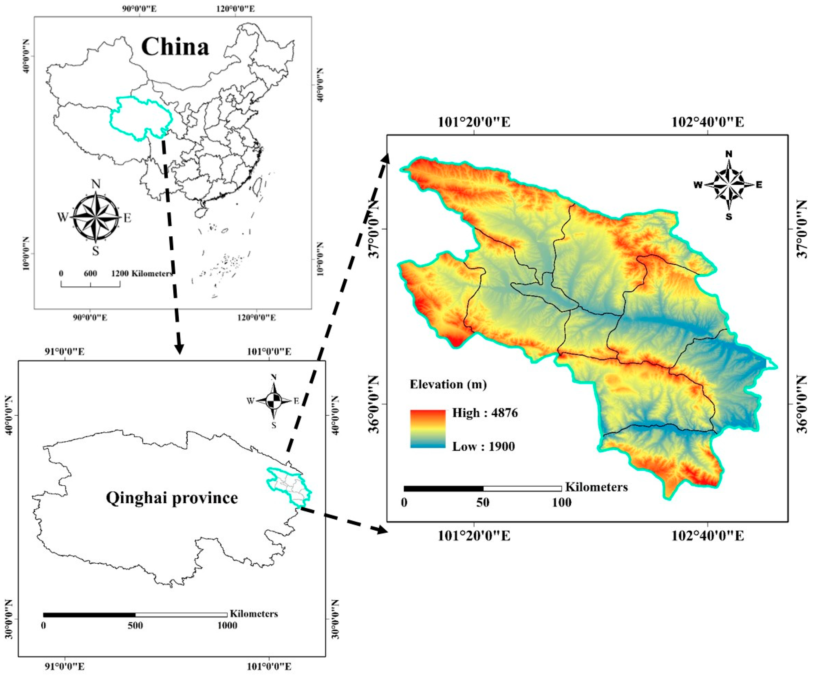
Figure 1. Location and topography of the study site, Xining and Haidong prefectures in Qinghai Province, China.
Remotesensing 17 03814 g001
Figure 2. The workflow of this study.
Remotesensing 17 03814 g002
Figure 3. The frequency of samples of various crop types in dataset 13 (Table 2) before and after 7:3 randomly train–test-split process by using scikit-learn 1.7.0 package under Python 3.12.3 (with random seed set as zero) (a) and the RF-RFE: number of variables vs. classification accuracy of the model based on training samples (b). The vertical line represents the threshold where the global accuracy is highest.
Remotesensing 17 03814 g003
Figure 4. Synthetic sample generation within the feature space using the ADASYN algorithm.
Remotesensing 17 03814 g004
Figure 5. The basic principle of DBSCAN clustering algorithm. In this example, mpt is set to two [48].
Remotesensing 17 03814 g005
Figure 6. The main workflow of ASROT algorithm. The m s and m l represent the sample size of minor and major classes, respectively.
Remotesensing 17 03814 g006
Figure 7. Accuracy measures for all datasets and two classifiers (stacking and RF models) prior to balancing: (a) OA and (b) macro F1-score value.
Remotesensing 17 03814 g007
Figure 8. OA vs. imbalance degree (a,b) and the macro F1-score value vs. imbalance degree (c,d) for RF and the stacking model prior to balancing. The superscript of “**” represents the extremely significant correlation, while the superscript of “*” represents the significant correlation.
Remotesensing 17 03814 g008
Figure 9. OA and macro F1-score for different resampling algorithms after balancing the datasets: (a,b) OA values for RF and stacking models and (c,d) macro F1-score values for RF and stacking models.
Remotesensing 17 03814 g009
Figure 10. Increase in (a,b) OA and (c,d) macro F1-score values after balancing the datasets for RF and stacking models.
Remotesensing 17 03814 g010
Figure 11. The Friedman test and the Nemenyi follow-up test of significance in the differences in the classification accuracies of the resampling algorithms for (a) RF and (b) stacking model. The black circles indicate the average ranking of each algorithm across the 13 datasets, and the bars are the critical values of the two-tailed test at the 95% significance level. The letters above lines represent the significance analysis of differences.
Remotesensing 17 03814 g011
Figure 12. Comparison of classification results between imbalanced and balanced training datasets after using the ASROT algorithm. (a,d) GF-6 images of two selected areas; (b,e) classification results with the original training dataset; and (c,f) classification results with the ASROT-balanced training dataset.
Remotesensing 17 03814 g012
Figure 13. F1-score of different crop types before and after ASROT algorithm balancing of the training datasets.
Remotesensing 17 03814 g013
Table 1. Summary characteristics of the GF-6 PMS sensor (China Aerospace Science and Technology Corporation, Beijing, China).
BandsNameWavelength Range (nm)Spatial Resolution (m)
PPanchromatic450–9002
B1Blue450–5208
B2Green520–600
B3Red630–690
B4NIR760–900
Table 2. Description of the 12 synthetic datasets and the original dataset, No. 13. The imbalance degree is defined in Equation (1). (HB stands for highland barley, and BB stands for broad beans).
DatasetCropsClass AllocationsTotal Samples (Pixels)Imbalance Degree
13Wheath–Rape–Maizel30002.95
23Wheath–Maizei–HBl40003.39
33Rapev–HBl–BBl55003.63
44Wheath–Rapel–Potatol–HBl32502.49
54Rapeh–Maizei–Potatoi–HBl52504.28
64Wheatv–Maizeh–HBi–BBl90004.32
75Wheati–Rapei–Potatol–BBl–Och55004.17
85Wheath–Rapel–HBh–Bbi–Ocv11,5004.60
96Wheatl–Rapel–Maizeh–HBh–BBh–Ocl82504.53
106Wheati–Rapeh–Maizei–Potatoh–Bbi–Oci10,0005.41
117Wheatv–Rapeh–Maizei–Potatoi–HBl–BBl–Och13,0005.67
127Wheati–Rapei–Maizeh–Potatoh–HBv–BBv–Oci18,7505.74
137Wheat–Rape–Maize–Potato–HB–BB–OC186,3814.68
Note: Subscripts represent the pixel count. l, i, h, and v represent 250, 1250, 2500 and 5000 samples, respectively. In dataset 13, the sample sizes of wheat, rape, maize, potato, HB, BB, and OC are 45,035, 43,067, 24,600, 30,424, 9142, 5373, and 28,740, respectively [10].
Table 3. Initial features used as inputs to the classifiers.
Type of FeatureFeatures Selected
Spectral bandsGreen (B2), Red (B3), NIR (B4)
Vegetation indicesGNDVI = (B4 − B2)/(B4 + B2),
TVI = 0.5 * [120 * (B4 − B2) − 200 * (B3 − B2)],
Texture featuresB1_Mean, B2_Mean, B3_Mean, B4_Mean
Topographic featuresElevation
Table 4. Changes in classification and identification of each crop class before and after using the ASROT algorithm.
ClassBefore Balancing DatasetAfter Balancing Dataset
UAPAF1-scoreUAPAF1-score
Wheat92.12%92.27%92.19%92.55%92.99%92.77%
Rape93.81%92.39%93.09%91.92%95.11%93.49%
Maize92.17%91.43%91.80%91.83%92.41%92.12%
Potato87.18%77.72%82.18%89.51%89.41%89.46%
BB57.95%68.67%62.86%87.02%84.32%85.65%
HB50.41%64.58%56.62%83.99%84.65%84.32%
Other87.35%89.81%88.56%88.80%92.79%90.75%
Disclaimer/Publisher’s Note: The statements, opinions and data contained in all publications are solely those of the individual author(s) and contributor(s) and not of MDPI and/or the editor(s). MDPI and/or the editor(s) disclaim responsibility for any injury to people or property resulting from any ideas, methods, instructions or products referred to in the content.