Article

Gully Extraction in Northeast China’s Black Soil Region: A Multi-CNN Comparison with Texture-Enhanced Remote Sensing

1
Jilin Province Technology Center for Meteorological Disaster Prevention, Changchun 130062, China
2
State Key Laboratory of Black Soils Conservation and Utilization, Northeast Institute of Geography and Agroecology, Chinese Academy of Sciences, Changchun 130102, China
*
Author to whom correspondence should be addressed.
Remote Sens. 2025, 17(23), 3792; https://doi.org/10.3390/rs17233792
Submission received: 28 September 2025 / Revised: 12 November 2025 / Accepted: 20 November 2025 / Published: 21 November 2025

Highlights

What are the main findings?
  • A GLCM-based texture enhancement method with a 5 × 5 window and 32 gray levels improves boundary detection in high-resolution imagery, boosting U-Net accuracy by 1.54% for erosion gully extraction.
  • Among DeepLabv3+, U-Net, and U-Net++, U-Net achieves the highest performance (90.27% accuracy with texture features), excelling in capturing elongated gully structures while reducing false positives.
What is the implication of the main finding?
  • The texture-fused U-Net framework enables scalable, automated gully monitoring in Northeast China’s black soil region, aiding timely soil erosion assessment without relying on DEM data.
  • Enhanced extraction accuracy supports sustainable land management and policy decisions for conserving fertile black soils, mitigating threats to agricultural productivity and food security.

Abstract

Gully erosion poses a serious threat to soil fertility and agricultural sustainability in Northeast China’s black soil region. Accurate and efficient mapping of erosion gullies is critical for enabling targeted soil conservation and precision land management. In this study, we developed a texture-enhanced deep learning framework for automated gully extraction using high-resolution GF-1 and GF-2 satellite imagery. Key texture parameters—specifically mean and contrast features derived from the gray-level co-occurrence matrix (GLCM) under a 5 × 5 window and 32 gray levels—were systematically optimized and fused with multispectral bands. We trained and evaluated three convolutional neural network architectures—U-Net, U-Net++, and DeepLabv3+—under consistent data and evaluation protocols. Results demonstrate that the integration of texture features significantly enhanced extraction performance, with U-Net achieving the highest overall accuracy (90.27%) and average precision (90.87%), surpassing DeepLabv3+ and U-Net++ by margins of 6.06% and 9.33%, respectively. Visualization via Class Activation Mapping (CAM) further confirmed improved boundary discrimination and reduced misclassification of spectrally similar non-gully features, such as field roads and farmland edges. The proposed GLCM–CNN integrated approach offers an interpretable and transferable solution for gully identification and provides a technical foundation for large-scale monitoring of soil and water conservation in black soil landscapes.

1. Introduction

The black soil region of Northeast China, one of the world’s four major black soil belts, is renowned for its fertile soils and serves as a vital national grain-producing area and a commercial grain base [1,2]. However, decades of intensive agricultural exploitation have resulted in severe soil and water loss [3]. Among the various forms of land degradation, gully erosion is particularly widespread and destructive. Recent survey data from the Ministry of Water Resources report that 666,700 gullies have already developed in this region [4]. These erosional features degrade soil quality, reduce crop yields, and ultimately threaten local livelihoods and the long-term sustainability of agriculture [5].
Accurate gully identification and extraction are prerequisites for dynamic monitoring and effective land management [6]. Remote sensing offers clear advantages in this regard, as it enables large-scale, multi-temporal, and high-resolution surface monitoring [7,8]. Traditionally, gully mapping has relied on manual visual interpretation of high-resolution imagery [9,10]. Although this method reduces the need for extensive fieldwork, it is inefficient, highly subjective, and inconsistent across interpreters [11,12], thereby rendering it unsuitable for large-scale, high-precision applications.
In recent years, automated approaches have been increasingly applied to gully extraction. Texture analysis methods, such as the Gray Level Co-occurrence Matrix (GLCM), quantify pixel-level spatial patterns and improve boundary discrimination between gullies and surrounding farmland [13]. GLCM has found mature applications in remote sensing imagery, topographic modeling, and soil type classification. For instance, Lan and Liu (2018) demonstrated in a multispectral image classification study that GLCM texture features, when combined with multi-scale windows and directional angle optimization, can substantially improve geographic scene classification accuracy [14]. Chen and Liu (2025) incorporated GLCM texture metrics when utilizing GF-2 satellite imagery for sloping farmland in black soil regions, combined with DEM/DSM data, thereby validating their potential value in erosion gully identification [13]. Furthermore, Moya et al. (2019) explored the advantages of 3D-GLCM (multi-layer imagery or band combinations) in complex landform recognition, highlighting the significant impact of grayscale levels, distance offsets and directional angles on texture description efficacy [15]. Empirically, the value of GLCM in gully extraction extends beyond providing texture evidence complementary to spectral information and mitigating spectrally similar linear features (e.g., roads and field ridges); it also furnishes structured priors for deep network inputs. With optimized parameters and fusion strategies, it enhances boundary discrimination finesse and overall accuracy. Meanwhile, deep learning techniques—particularly convolutional neural networks (CNNs)—have demonstrated remarkable performance in semantic segmentation of remote sensing imagery [16,17]. Architectures such as U-Net, DeepLabv3+, and U-Net++ are well suited for extracting small-scale, elongated, and boundary-blurred features by integrating multi-scale contextual information [18,19,20,21]. Empirical studies further highlight these strengths. For example, Li et al. (2023) improved DeepLabv3+ with edge features and multi-level upsampling to enhance segmentation of elongated objects [22], while Chen et al. (2021) used an AdaBoost-like ensemble of lightweight U-Nets to extract narrow linear features with fewer discontinuities [23]. Zhao et al. (2025) embedded residual dual attention and multi-scale context modules into a Nested U-Net++, achieving excellent results in segmenting cracks and textured pavement surfaces [24]. In the context of gullies, Zhang et al. (2024) modified DeepLabv3+ to improve boundary detection in farmland imagery [19], and Li et al. (2024) proposed the Gully-ERFNet model, which achieved 87.54% accuracy using only GF-2 imagery without relying on DEM data [25].
Despite the application of convolutional neural networks (CNNs) and gray-level co-occurrence matrices (GLCMs) in remote sensing for land cover and landform recognition, research on texture features specifically tailored to the prevalent gully erosion landforms in the black soil region of Northeast China remains insufficient. On one hand, substantial studies have addressed the distribution, evolution, and driving factors of gully erosion in the region [26,27,28,29,30]; however, systematic reviews and comparisons of the integration of remote sensing imagery with texture features for gully erosion extraction, from the perspective of input feature engineering, remain inadequate. On the other hand, current research predominantly focuses on innovations in network architectures, with limited attention to tight coupling strategies between classical texture descriptors such as GLCM and deep networks, as well as their parameterized optimization. From a practical perspective, two key challenges persist: first, the spectral similarity between gullies and adjacent linear features such as field roads and crop boundaries often results in blurred boundaries and misclassification; second, trade-offs between multi-scale contextual information and fine-grained structural details across different CNN frameworks lead to inconsistent performance, and the application of model interpretability for pinpointing error sources remains underdeveloped.
Against this backdrop, this study adopts a texture feature input perspective to address the co-occurrence of fine linear structures and background interference in black soil gully imagery, thereby constructing a texture-enhanced deep segmentation framework tailored to Northeast China’s black soil region (see Figure 1): on high-resolution multispectral imagery, systematic optimization of the GLCM parameter family (window size, grayscale levels, directional/distance offsets, and statistical metric subsets) yields interpretable and reproducible experimental factors [31,32]; the optimal texture subsets are fused with original spectral bands at the input stage, followed by parallel comparisons across mainstream CNN architectures (e.g., U-Net, U-Net++, DeepLabv3+), with Class Activation Mapping (CAM) employed to mechanistically analyze discriminative regions under varying input combinations, thereby pinpointing primary causes of false positives and detail omissions. This framework offers a transferable paradigm for texture parameter optimization and model comparison at the technical level, while providing interpretable spatiotemporal evidence and decision support for soil and water conservation, arable land protection, and precision monitoring in black soil regions at the application level. Accordingly, the innovations of this study are threefold: (1) GLCM parameter optimization: a reusable parameterization and subset selection workflow for GLCM, oriented toward structural scales and texture anisotropy in black soil gully imagery; (2) multi-model comparison under texture enhancement: under unified data and evaluation protocols, contrasting “spectral-only CNN” with “texture-enhanced CNN fusion models” to quantify texture gains rather than mere architectural replacements; (3) empirical validation and interpretability in black soil regions: validation in representative black soil areas, coupled with interpretability analysis of optimal results, to furnish a transferable technical roadmap for subsequent regional automated mapping and land management.

2. Materials and Methods

2.1. Study Area and Data Source

2.1.1. Study Area

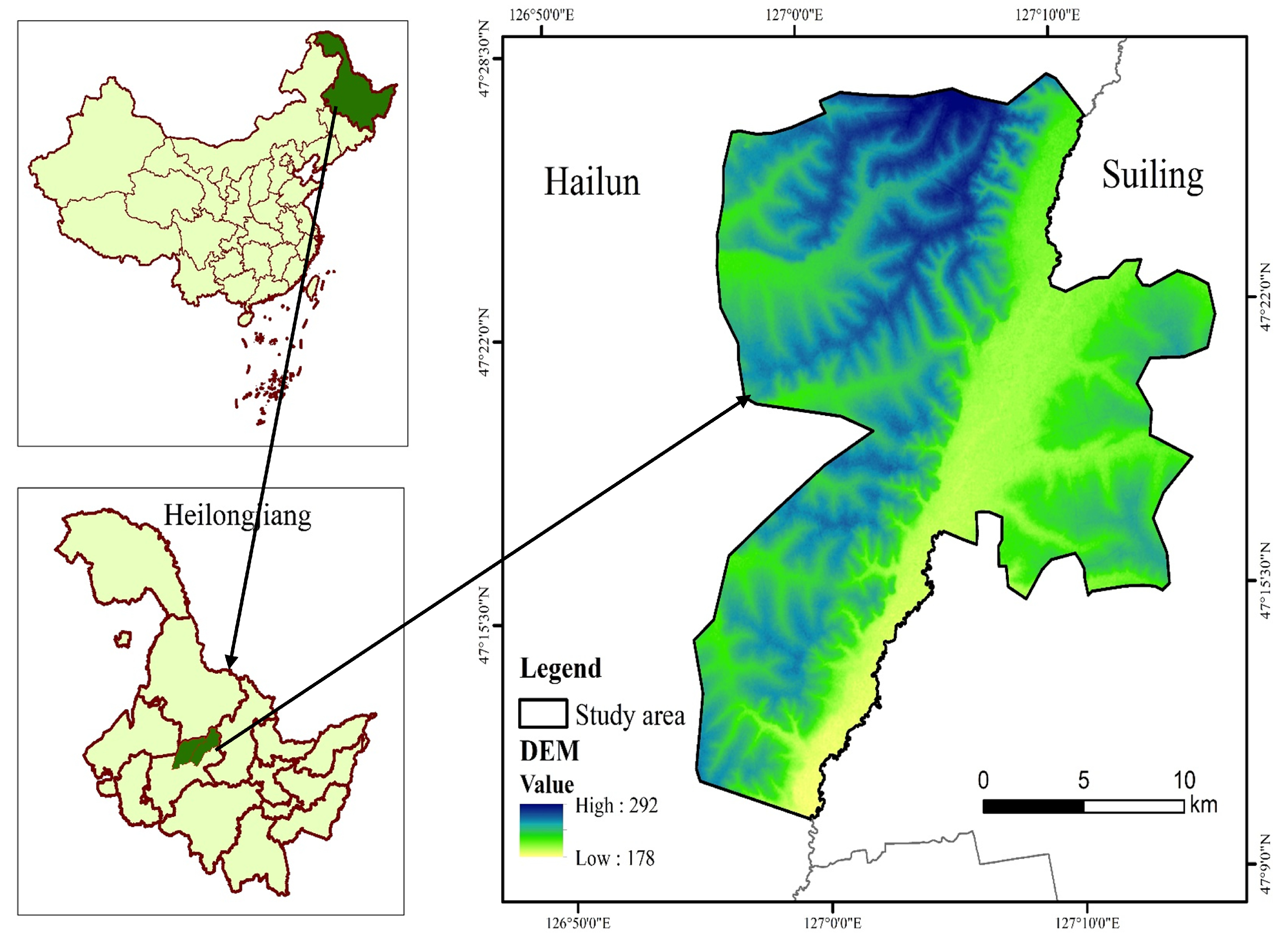
This study focused on the core area of the typical black soil belt in Northeast China (Figure 2), encompassing Dongfeng Town and Hainan Township in Hailun City, Heilongjiang Province, as well as Keyinhe Township in Suiling County. The landform of this region follows a general pattern of “high in the west and low in the east,” with topography ranging from low-lying plains (<180 m) and gently undulating uplands (180–240 m) to hilly uplands (>240 m). The climate is cold and dry, with distinct seasonal variation. The mean annual temperature is 2.0–2.5 °C, and average annual precipitation is about 550 mm [33].
The unique geographical and climatic conditions, combined with the widespread distribution of fertile black soil, provide a highly favorable environment for agricultural production. The black soil layer is deep, loose, and well-aerated, with strong water- and nutrient-retention capacity, creating optimal conditions for crop growth. Cultivated farmland dominates land use, with maize and soybeans as the principal crops [5].
In recent decades, however, intensive farming practices characterized by “high utilization with insufficient replenishment” have accelerated soil and water loss. This has resulted in extensive gully development, which reduces the efficiency of agricultural mechanization, disrupts cropping patterns, and poses a potential threat to regional food security [34,35].
Given its representative topography, farming patterns, and natural conditions, the selected study area reflects the broader background of gully development and agricultural land use across the thick-layer black soil region of Northeast China [35].

2.1.2. Data Source and Preprocessing

A total of six high-resolution remote sensing images were used in this study, including four GF-1 images and two GF-2 images, provided by the Satellite Environment Center, Ministry of Ecology and Environment of China (http://www.secmep.cn (accessed on 18 June 2023)). All data were orthorectified TIFF products referenced to the WGS 1984 geographic coordinate system. The panchromatic spatial resolutions of GF-1 and GF-2 imagery are 2 m and 0.8 m, respectively, and the multispectral spatial resolutions are 8 m and 3.2 m, respectively. To minimize vegetation interference and highlight surface structures, all images were acquired during typical non-cropping periods: GF-1 images on 14 November 2020, and GF-2 images on 4 November 2022.
Preprocessing was conducted in ENVI 5.6. Prior to fusion, radiometric calibration was performed to convert the digital numbers (DNs) of each band to at-sensor radiance using sensor-specific calibration coefficients provided by the data supplier. Subsequently, atmospheric correction was applied using the Fast Line-of-sight Atmospheric Analysis of Spectral Hypercubes (FLAASH) module to obtain surface reflectance. To ensure inter-sensor comparability, spectral calibration was carried out by aligning the spectral response functions of corresponding GF-1 and GF-2 bands based on published sensor parameters. Following radiometric and spectral normalization, pan-sharpening was performed using the Gram–Schmidt fusion method, fusing GF-1 multispectral bands from 8 m to 2 m and GF-2 multispectral bands from 3.2 m to 0.8 m. To standardize spatial resolution, the pan-sharpened GF-1 imagery was further resampled to 0.8 m using cubic convolution, ensuring consistency with GF-2 data. Geometric correction was implemented using the “Image-to-Image Registration” tool in ENVI, with GF-2 imagery serving as the reference. A set of well-distributed ground control points was selected to co-register the GF-1 and GF-2 datasets, achieving a registration accuracy of <0.5 pixels. All training and validation samples were subsequently extracted from the co-registered multispectral fused images with a unified spatial resolution of 0.8 m, ensuring consistency in spatial scale and radiometric characteristics across all datasets.

2.2. Texture Feature Extraction of Gray-Level Co-Occurrence Matrix Images

2.2.1. Texture Feature Extraction

Texture is the integrated expression of an object’s surface details and visual characteristics, reflecting its morphology, structure, and variation patterns [36]. It comprises multiple elements—such as color, brightness, shape, size, and orientation—that may appear in either regular or random distributions within an image [37]. In practice, texture recognition does not directly employ GLCM. Instead, statistical features derived from the GLCM are calculated and used as the basis for classification or discrimination [38,39].
In this study, two GLCM-based statistical features—contrast and mean—were selected as key parameters. Contrast captures gray-level variations, emphasizes edge information, and enhances the representation of linear structures, which is particularly valuable for identifying elongated landforms such as gullies. Mean reflects the gray-level difference between gully areas and their surrounding background, thereby improving target-to-background separability and facilitating accurate gully localization and segmentation.
The GLCM feature formulas are expressed as follows:
① Contrast:
C O N = i = 0 n j = 0 n i j 2 p i , j
Here, n denotes the number of gray levels in the image, p i , j represents the value of the element i , j in the GLCM.
② Mean:
M E A N = i = 0 n i ( j = 0 n p ( i , j ) )
Here, n denotes the number of gray levels in the image, p i , j represents the value of the element i , j in the GLCM, that is, the probability of occurrence of the pixel pair i , j .

2.2.2. Principal Component Analysis

Principal Component Analysis (PCA) is a widely applied dimensionality reduction technique designed to reduce the number of variables in a dataset while preserving its most critical information [40]. Its primary objective is to project the original data into a new feature space, generating components that capture the maximum variance within the dataset [41]. This transformation not only enhances data visualization and interpretation but also decreases computational complexity and simplifies subsequent model operations. By extracting the most informative features, PCA effectively reduces dimensionality while retaining the majority of the dataset’s informational content [42].
The specific algorithm is as follows:
① Let the original image be denoted as x , where each band image is represented by the rows of a matrix. Let M be the number of bands in the image, and N be the number of pixels in each band. The expression is as follows:
x = x 11 x 12 x 1 N x 21 x 22 x 2 N x M 1 x M 2 x M N
② Perform standardization processing. Calculate the mean x - j = 1 m i = 1 m x i j and standard deviation by column S j = i = 1 m x i j x - j 2 m 1 , Calculate the standardized data X i j = x i j x - j S j , The metadata after standardization is:
  x = x 11 x 12 x 1 n x 21 x 22 x 2 n x m 1 x m 2 x m n
③ Calculate the covariance matrix R, as follows:
R = 1 n X X I [ X X I ] T I = 1,1 , , 1 1 × n ,   X - = x 1 , x - 2 , , x - n T x i = 1 n k = 1 n x i k
④ Solve the characteristic equation to generate the transformation matrix.
λ I R U = 0
In the above formula, after calculating the eigenvalues and eigenvectors, the transformation matrix is constructed. The matrix composed of the eigenvectors is denoted as U, and its transpose matrix U is the transformation matrix, denoted as T. At this point, the following formula is used:
Y = T X

2.2.3. Setting the Sliding Window Sizes and Gray Levels

After determining the appropriate GLCM image band, a series of comparative experiments were conducted to systematically evaluate the effects of different window sizes (5 × 5 and 7 × 7) and gray levels (16, 32, 64) on texture feature extraction.
These parameter ranges were selected based on both theoretical considerations and empirical evidence from previous studies. The determination of the GLCM window size was guided by the principle of matching the spatial scale of the analysis unit to the morphological scale of gullies. Very small windows (e.g., 3 × 3) tend to lack contextual information and cannot capture the linear continuity and boundary transitions typical of gully forms, while overly large windows (e.g., 9 × 9) may oversmooth edges and incorporate irrelevant background information, thereby reducing discriminative power [14,43,44].
Similarly, the quantization of gray levels directly affects the stability and sensitivity of co-occurrence statistics. Overly coarse quantization (≤8 levels) leads to information loss and quantization noise, whereas excessively fine quantization (≥128 levels) results in matrix sparsity and amplifies random fluctuations. Multiple studies have demonstrated that the range of 16–64 gray levels achieves an optimal balance between statistical robustness and feature detail preservation [43,45,46].
Accordingly, the present study adopted 5 × 5 and 7 × 7 windows and 16–64 gray levels as the experimental parameter range. GLCM calculations were applied to the high-resolution imagery, and the optimal combination was identified through a comprehensive evaluation that integrated qualitative visual analysis with quantitative performance metrics [39,47]. The goal was to ensure that the final parameters not only enhanced the spatial representation of gullies but also effectively suppressed background noise, thereby improving both the accuracy and robustness of the subsequent model training [48].

2.3. Sample Set Construction

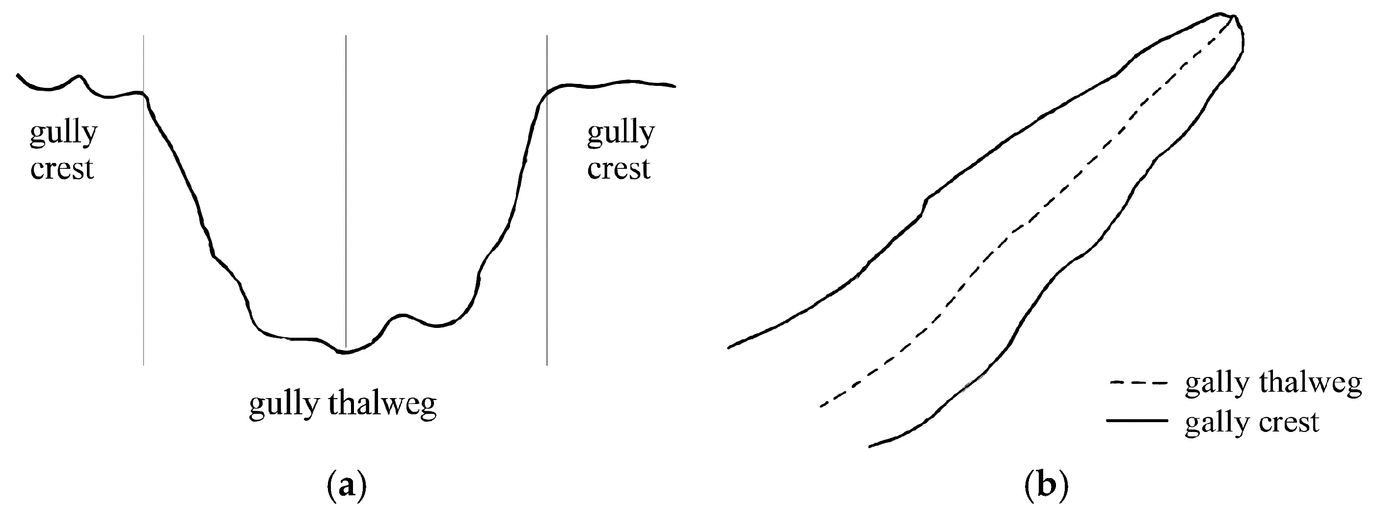
As a typical fluvial erosion landform, gullies can be characterized by their thalweg and crest lines, which effectively represent their spatial morphology. In this study, manual visual digitization was employed to annotate gully crest lines. Continuous delineation was performed along both sides of each gully to ensure complete boundary coverage (Figure 3). This approach offers clear advantages: it accurately captures the morphology, scale, and geographic distribution of gullies, thereby providing precise inputs for morphological observation and feature analysis. It also enhances the model’s ability to recognize elongated landform targets. However, the method has limitations, as delineating irregular boundaries is complex, subjective, time-consuming and resource-intensive.
Based on this annotation method, typical gully areas and background areas were randomly sampled across the study region. A total of 1175 independent gully polygon samples were obtained from traditional high-resolution imagery, and 1141 samples were extracted from the high-resolution composite texture feature imagery, together forming the gully sample set.
To ensure the reliability of interpretation results, stratified random sampling was applied after visual interpretation of the high-resolution imagery. At least 10% of the total samples were selected as validation samples. Stratification was based on major land cover types and gully density zones, ensuring representativeness across geomorphic units. Field validation was conducted using high-precision GPS positioning, supported by on-site photography and field records, to compare against the interpreted results. Validation confirmed that the overall accuracy of gully extraction exceeded 95%, meeting the precision requirements for subsequent CNN model training.

2.4. Convolutional Neural Networks

2.4.1. U-Net Network
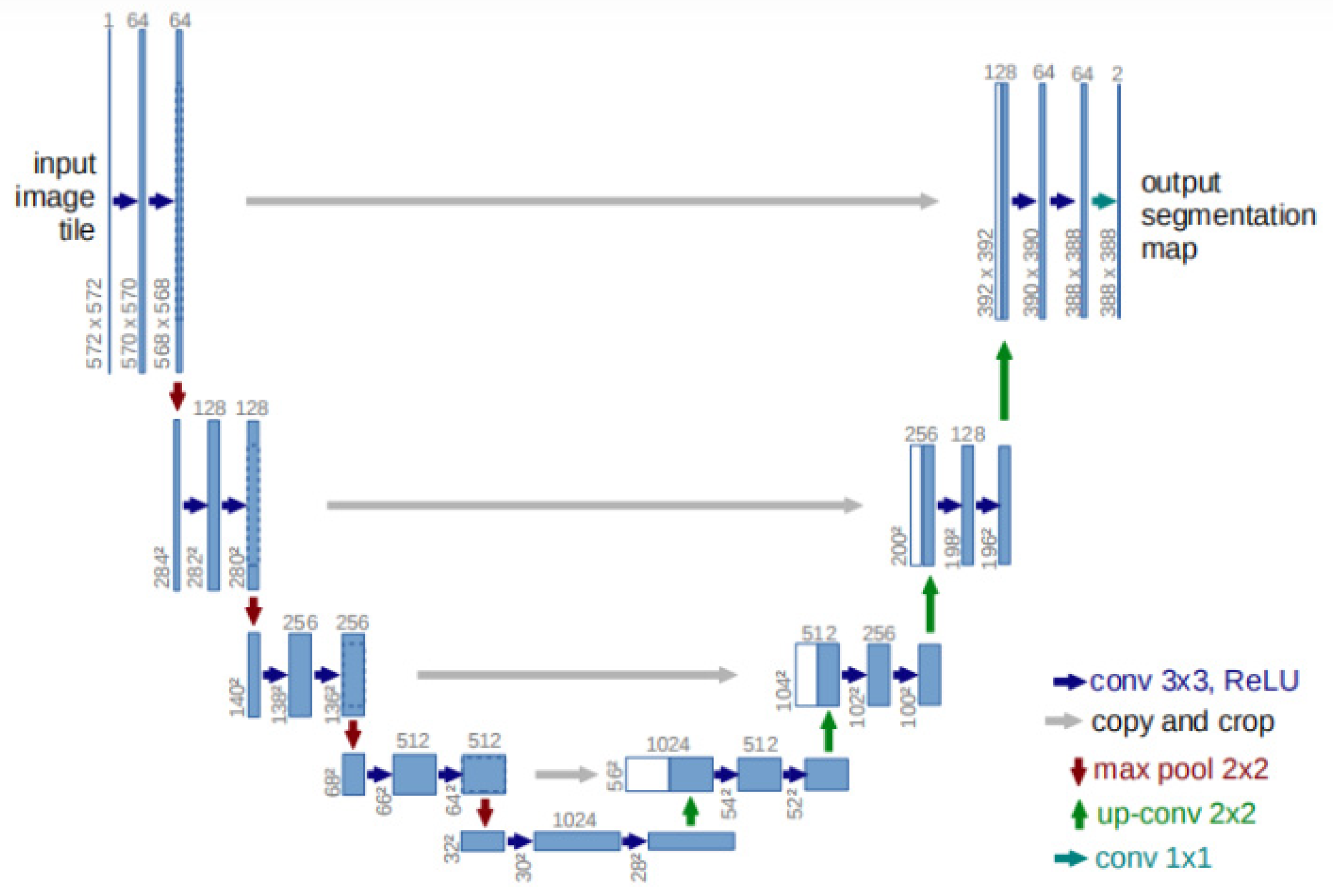
The U-Net network is a deep learning architecture specifically designed for image segmentation tasks. As illustrated in Figure 4, its defining characteristic is the U-shaped symmetrical structure formed by an encoder–decoder framework [49]. The encoder, located on the left, progressively extracts features through stacked convolutional and pooling layers, reducing spatial resolution while increasing the number of feature channels. The decoder, on the right, employs transposed convolution layers to gradually restore the feature maps to the original image size.
A major strength of U-Net lies in its skip connection mechanism, which links corresponding encoder and decoder layers. These connections integrate low-level spatial details with high-level semantic features, facilitating accurate boundary delineation and detail preservation [50]. Due to this design, U-Net is particularly effective for segmentation tasks involving small sample sizes, class imbalance, or requirements for retaining fine structural details [51].
Figure 4. U-Net network architecture (redrawn from Ronneberger et al., 2015 [52]).
Remotesensing 17 03792 g004

2.4.2. U-Net++ Network

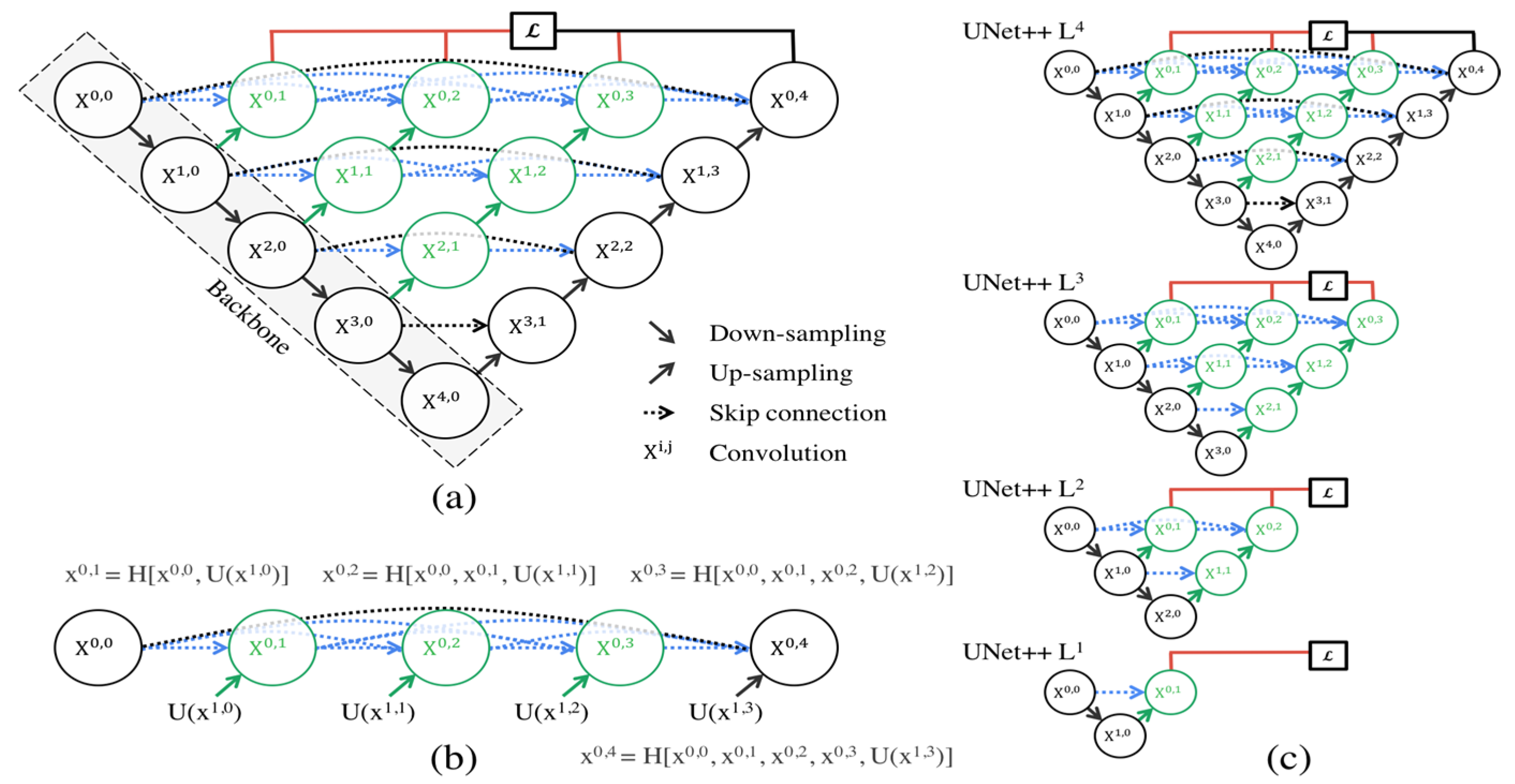
U-Net++ is an enhanced variant of the U-Net architecture, developed to improve the accuracy and robustness of image segmentation tasks [18]. Unlike the original U-Net, U-Net++ incorporates dense skip connections, which introduce multiple intermediate bridging layers between the encoder and decoder. This design strengthens multi-scale feature fusion and facilitates more effective information flow across the network. In addition, U-Net++ applies a nested deep supervision mechanism, in which loss functions are introduced at different resolution levels. This strategy enhances feature learning across all layers, improving both accuracy and convergence stability.
The architecture is more flexible than U-Net and can be adapted to diverse tasks and datasets, making it highly robust and versatile. Owing to these improvements, U-Net++ has shown excellent performance in remote sensing image processing and has become one of the preferred models for high-precision segmentation tasks. The detailed structure is illustrated in Figure 5.

2.4.3. DeepLabv3+ Network

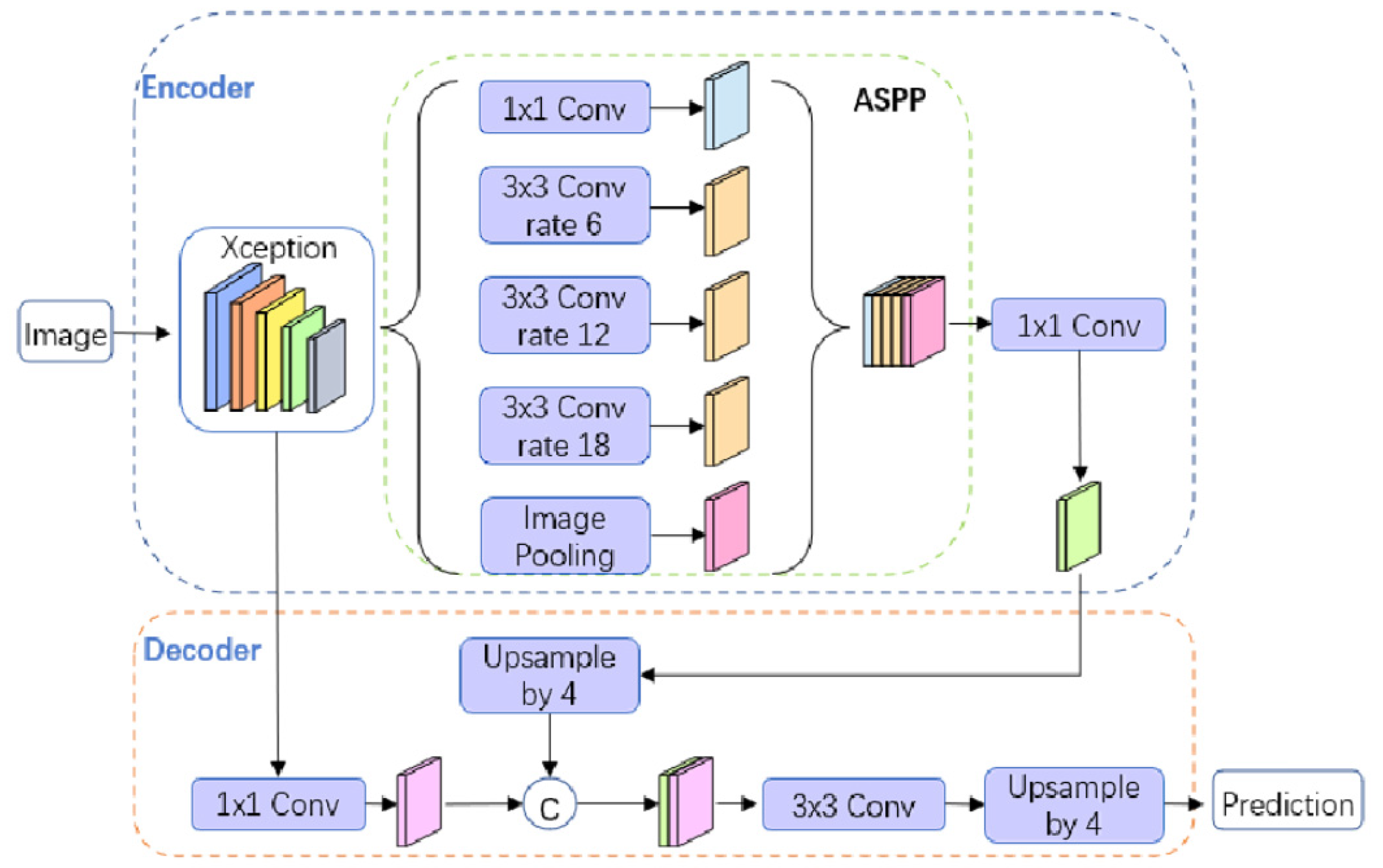
DeepLabv3+ is an advanced semantic segmentation model that extends DeepLabv3 by integrating spatial pyramid pooling with an encoder–decoder structure [54]. The addition of the encoder–decoder architecture enables the model to better capture fine details and boundary information, thereby improving segmentation accuracy. In the encoder, DeepLabv3+ retains the backbone of DeepLabv3, employing atrous (dilated) convolution to enlarge the receptive field and effectively capture multi-scale contextual information. The decoder then progressively restores spatial details, producing segmentation outputs that are more refined and precise.
With its strong feature extraction ability and superior detail restoration, DeepLabv3+ has demonstrated excellent performance across a wide range of semantic segmentation tasks and is now considered one of the mainstream models in the field [55]. The detailed architecture is illustrated in Figure 6.

2.4.4. Model Training Settings

To ensure a fair comparison among the CNN models (U-Net, U-Net++, and DeepLabv3+), all were trained using identical strategies under the same hardware environment. The training hyperparameters were configured as follows: the initial learning rate was 0.001, batch size was 8, patch sampling rate was 16, and the maximum number of iterations was set to 100 epochs. The dataset was split into training and validation sets at a ratio of 8:2. To improve model generalization, data augmentation techniques—including random rotation and random scaling—were applied during training.
All experiments were conducted on a Windows operating system equipped with an Intel i9 processor and an NVIDIA RTX 3080 GPU. The models were implemented in Python 3.8 using the TensorFlow 2.4 framework, with preprocessing supported by the ENVI platform. On this setup, each training epoch required approximately 2–5 min to complete.

2.5. Accuracy Evaluation

To evaluate the accuracy of model inversion, this study used the validation dataset and selected accuracy (Acc) (Equation (8)), average precision (AP) (Equation (11), Intersection over Union (IoU) (Equation (12)), and loss function value (Loss) as assessment metrics.
A c c u r a c y = T P + T N T P + T N + F P + F N
P = T P T P + F P
R = T P T P + F N
A P = 0 1 P R d R
I o U = T P T P + F N + F P
where
  • TP—Number of samples correctly predicted as positive;
  • TN—Number of samples correctly predicted as negative;
  • FP—Number of samples incorrectly predicted as positive;
  • FN—Number of samples incorrectly predicted as negative.
Loss Function Value (Loss)—an important metric for measuring the difference between the model’s predictions and the actual results [57]. A smaller loss value indicates that the model’s predictions are closer to the true outcomes.

2.6. Visualization and Interpretation of Model Decisions Based on Class Activation Mapping

Class Activation Mapping (CAM) is a visualization technique widely used in CNN interpretability studies to identify the spatial regions that influence a model’s predictions in image classification or segmentation tasks [58]. By combining prediction scores for a target class with feature maps through weighted fusion, CAM produces a heatmap that highlights the areas most relevant to the model’s decision-making, thereby revealing its attention focus [58,59].
In this study, CAM was applied to the trained U-Net model to assess whether the network accurately concentrated on gully regions, thereby evaluating its feature extraction capability and potential risk of misclassification [59]. Specifically, the final convolutional feature maps were linearly combined with the corresponding class weights to generate a response map for the gully class. This map was normalized and superimposed on the original imagery to create a spatial heatmap [58]. CAM analysis not only provides intuitive evidence for evaluating model performance but also helps identify common sources of error, such as field roads, farmland boundaries, and narrow river channels that share spectral and morphological similarities with gullies. These insights offer both theoretical and practical guidance for subsequent model refinement and optimization [59].

3. Results and Analysis

3.1. Optimization and Analysis of Texture Feature Parameters

3.1.1. Band Statistical Analysis and Principal Component Analysis

(1) Band Statistical Analysis
Table 1 summarizes the statistical results of different bands under the GLCM-derived mean and contrast features. Regarding the mean feature, Bands 2 and 3 exhibit higher maximum values (2.8840 and 2.8360, respectively) than Band 1, indicating a richer distribution of average gray levels. Band 3, in particular, shows the largest standard deviation (1.8462), reflecting stronger internal variation in its mean gray levels. This suggests an enhanced ability to represent texture gradation, which can improve the model’s capacity to capture topographic undulations and object boundaries. A larger standard deviation indicates greater dispersion of brightness values from the mean, which corresponds to stronger differentiation between objects and thus richer information content [39]. In contrast, Band 1 shows the smallest variation in mean values, suggesting relatively limited texture information and weaker applicability.
Regarding the contrast feature, Band 3 again stands out. It has the widest gray-level range (0–159), far exceeding that of Bands 1 and 2, and a standard deviation of 0.3849, indicating the most dispersed gray-level distribution. This enhances its ability to capture pronounced differences between objects and to highlight linear structures and boundaries. Band 1, by contrast, shows the weakest variation in contrast (standard deviation: 0.2804), making it less effective for distinguishing fine texture details.
Comparison of the two texture features demonstrates that Band 3 possesses the strongest capacity for information representation and object differentiation. It more effectively emphasizes gray-level boundaries and texture characteristics of linear landforms such as gullies. For this reason, Band 3 was selected as the primary band for subsequent texture feature extraction and composite imagery construction, supported by both theoretical rationale and empirical evidence.
(2) Principal Component Analysis
Table 2 presents the principal component values of each band after PCA processing under the mean and contrast texture features of the remote sensing imagery. For the mean feature, Band 3 exhibits the largest eigenvalue for the first principal component (Eig.1 = 0.5315), exceeding those of Band 1 (0.4198) and Band 2 (0.4271). This indicates that Band 3 carries the most information for representing local gray-level distributions and texture variation. The third principal component of Band 3, however, is negative (−0.7087), suggesting that it primarily reflects noise or low-correlation features with minimal informational value. This result implies that the mean feature in Band 3 is strongly concentrated in the first principal component, demonstrating a higher feature aggregation capacity.
For the contrast feature, Band 3 again performs best, with the highest first principal component value (5.0300), surpassing Band 1 (4.9500) and Band 2 (5.0200). This confirms its superior ability to capture gray-level contrast and structural edge information. The second (−4.2500) and third (−1.4000) components show distinctly negative values, further indicating that they mainly represent noise and contribute little meaningful information.
Overall, Band 3 demonstrates the strongest variance explanatory power in the first principal component for both texture features, with a sharp decline in information content in subsequent components, indicating high redundancy. Therefore, the first principal component image of Band 3 was selected as the final texture feature image. This selection reduces data dimensionality while preserving the most critical surface texture information, thereby providing essential support for gully boundary and morphology identification. To minimize computational cost, the first principal component image of Band 3 was used as the GLCM feature input in the subsequent experiments.

3.1.2. Determination of Optimal GLCM Parameter Combination

To improve the separability of gullies from background objects, GLCM mean and contrast images were generated in ENVI using various combinations of sliding window sizes (5 × 5, 7 × 7) and gray levels (16, 32, 64). For both gully and background areas, the mean gray value difference (ΔMean) and the background standard deviation (Std) were calculated. Here, ΔMean = (Gully Mean − Background Mean) quantifies target–background separability, while Std reflects the level of texture noise. The results are summarized in Table 3.
In the GLCM mean images, the mean gray value of gullies was consistently lower than that of the background across all parameter combinations, yielding negative ΔMean values (e.g., ΔMean = −1.8602 for 5 × 5/32). This indicates that gullies have lower overall gray-level textures compared with their surroundings. Although this pattern contrasts with the conventional “higher target response” assumption in image processing, it is reasonable in the context of Northeast China’s black soil region. Gullies often occur as bare, low-lying, or water-accumulated areas, characterized by concentrated gray levels and relatively stable texture variation. In contrast, surrounding farmland is influenced by plowing marks, ridge–furrow structures, and crop residues, producing more complex gray-level distributions and higher texture values. Consequently, in GLCM mean images, farmland appears “brighter” than gullies. This observation aligns with earlier findings (Table 1 and Table 2), confirming the structural characteristic of gullies as “distinct boundaries but lower mean texture values.”
Among different parameter combinations, the magnitude of ΔMean increased with higher gray levels. For example, under a 5 × 5 window, ΔMean rose from −0.8657 at 16 gray levels to −3.7273 at 64 gray levels, suggesting improved separability. However, background Std also increased substantially (from 0.5905 to 2.7040), introducing higher noise—particularly at 64 gray levels, where non-target interference was evident. The 5 × 5 window + 32 gray-level combination provided the best balance between separability and noise (ΔMean = −1.8602, Std = 1.3374) and was therefore considered optimal.
In the GLCM contrast images, most ΔMean values were positive, indicating that gullies exhibited greater gray-level contrast, consistent with their geomorphic traits of “sharp edges and abrupt changes.” For example, under a 5 × 5 window at 32 gray levels, ΔMean reached 0.2195—higher than −0.5186 at 16 gray levels—while the background Std was only 0.1639, the lowest among all combinations. This suggests that the 32 gray-level setting enhanced target detectability while suppressing false responses from non-target backgrounds. Although ΔMean was higher at 64 gray levels (0.6519), the corresponding Std also increased (0.3896), producing fragmented textures and blurred boundaries that reduced stability. The 7 × 7 window generally performed less effectively; for instance, at 32 gray levels, ΔMean was 0.2204, but the background Std rose to 1.3239, likely due to boundary blurring and local averaging that weakened texture discrimination.
The 5 × 5 sliding window with 32 gray levels demonstrated superior performance in both mean and contrast images. In the mean image, it achieved ΔMean = −1.8602 and Std = 1.3374, while in the contrast image it yielded ΔMean = 0.2195 and Std = 0.1639. This parameter combination provided the optimal balance between boundary clarity and noise control and was therefore adopted for constructing the final texture feature images.
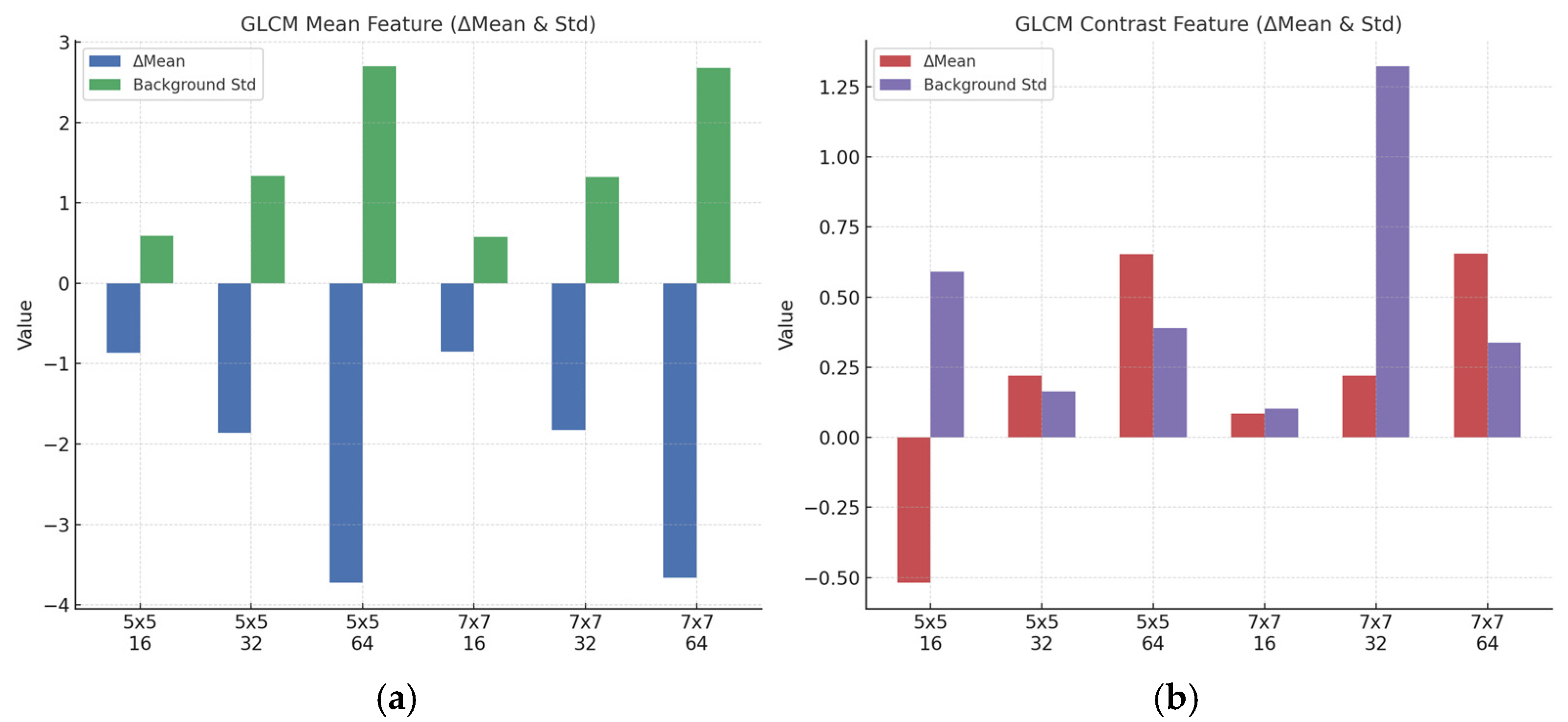
To further evaluate the recognition capability of gullies and the background suppression performance of different texture feature types, bar charts of ΔMean and background standard deviation (Std) were plotted for both GLCM mean and contrast images (Figure 7). In these charts, ΔMean represents the separability between gully and background responses, while Std reflects the noise level in the background. Together, they provide a comprehensive measure of discriminability and robustness.
In the mean feature images (Figure 7a), ΔMean values were negative for all parameter combinations, indicating that gully areas consistently exhibited lower average gray levels than the background. This result is consistent with the statistics presented in Table 1 and Table 2. Due to their recessed morphology, sparse vegetation, and exposed soil, gullies display concentrated gray-level distributions and lower average texture intensity. By contrast, surrounding farmland shows higher texture values, influenced by plowing marks and ridge–furrow structures. Among the tested parameter combinations, the 5 × 5 window with 32 gray levels achieved the most balanced separation (ΔMean = −1.8602, Std = 1.3374). At 64 gray levels, although ΔMean decreased further (−3.7273), the Std sharply increased (2.7040), resulting in texture fragmentation.
In the contrast feature images (Figure 7b), most ΔMean values were positive, demonstrating that gullies exhibit higher gray-level contrasts and more distinct edge expression. The 5 × 5 window with 32 gray levels again performed best, yielding ΔMean = 0.2195 and Std = 0.1639. This was the only configuration to combine positive texture enhancement with minimal background noise. By contrast, the 7 × 7 window with 32 gray levels produced a slightly higher ΔMean (0.2204), but the background Std rose markedly to 1.3239, reflecting noise instability caused by texture smoothing and boundary blurring at larger window sizes.
These results quantitatively confirm the earlier ROI-based findings, showing that the 5 × 5 window with 32 gray levels provides strong target–background separability and stable background performance in both mean and contrast images. This parameter set was therefore adopted for subsequent texture image construction and model training.
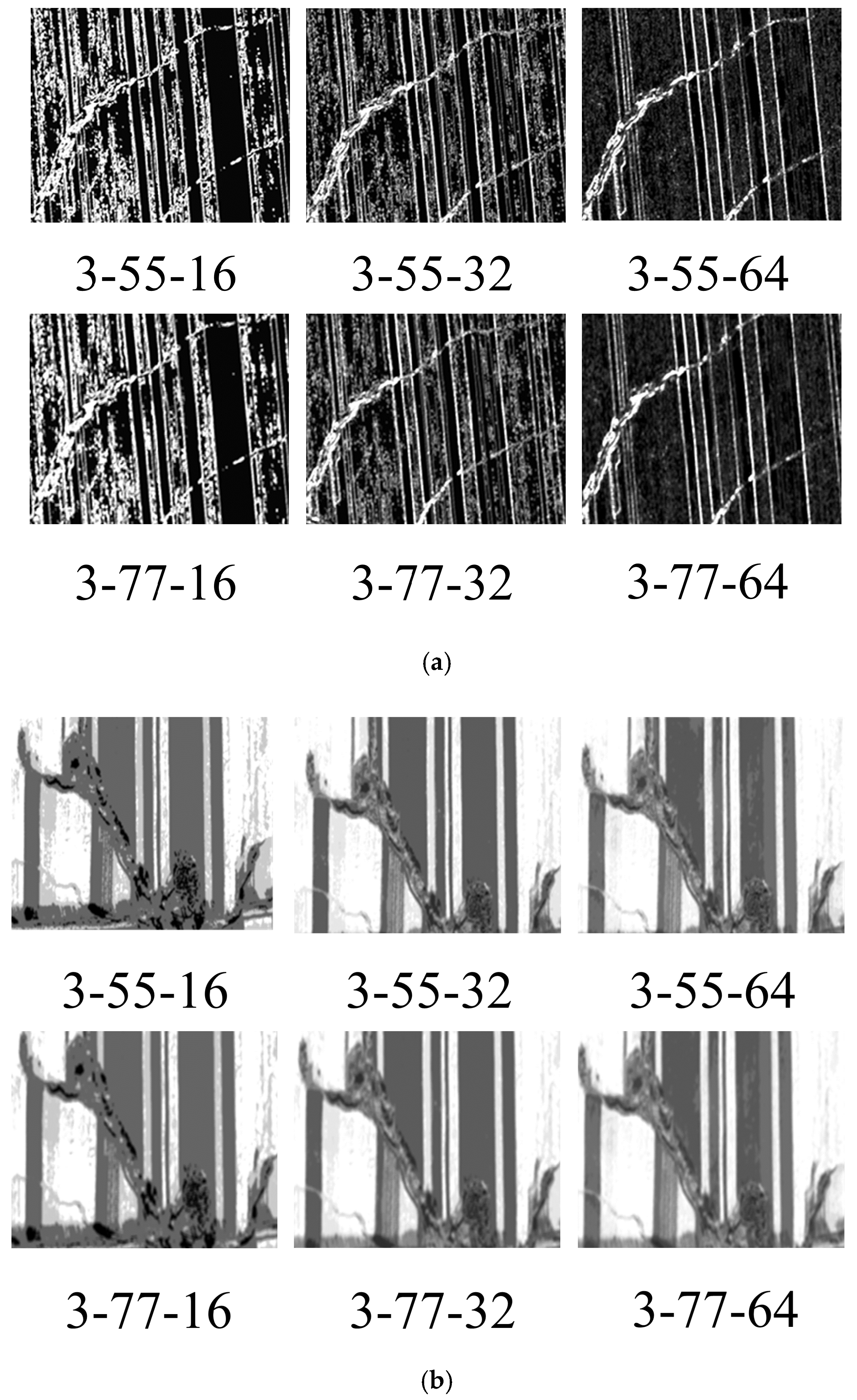
Figure 8 illustrates GLCM texture images derived from Band 3 under different parameter combinations of window size (5 × 5, 7 × 7) and gray levels (16, 32, 64). Both contrast (Figure 8a) and mean (Figure 8b) features are shown. The comparison demonstrates that parameter variations substantially affect the appearance of the texture images, influencing both gully boundary sharpness and the preservation of fine details.
For contrast features, higher gray levels (e.g., 64) strengthened gray-level differences but also introduced noise, leading to exaggerated boundaries and false textures in fine areas. Lower gray levels (e.g., 16) reduced noise but at the cost of detail, often obscuring narrow gullies [60]. The 32 gray-level configuration offered the best balance, maintaining clarity while controlling noise.
Window size also played a critical role. The smaller 5 × 5 window enhanced fine textures, making it more effective for detecting narrow gullies with sharp edge variations [39]. The larger 7 × 7 window produced smoother images but blurred boundaries and weakened texture detail, which is less suitable for segmenting fine-scale features [44,61]. Similar trends were observed in the mean feature images. Under the 5 × 5 window with 32 gray levels, the difference between gully and background gray levels was most pronounced, with moderate contrast and clear boundaries that supported accurate gully localization.
Based on these findings, this study selected high-resolution Band 3 imagery with a 5 × 5 sliding window and 32 gray levels for GLCM texture feature extraction. This configuration provides the best balance between enhancing gully spatial details and suppressing background noise, thereby offering more discriminative input features for subsequent deep learning models.
To improve the model’s recognition capability, texture images derived from different statistical measures were fused with multispectral bands of the original remote sensing imagery. After preprocessing, these data layers were integrated to generate a high-resolution composite image. The composite image provides a more comprehensive representation of surface information, enhancing the model’s ability to capture fine spatial details and thereby improving the accuracy of gully and surface feature extraction.

3.2. Comparison Between Texture-Enhanced Composite Imagery and Original Imagery

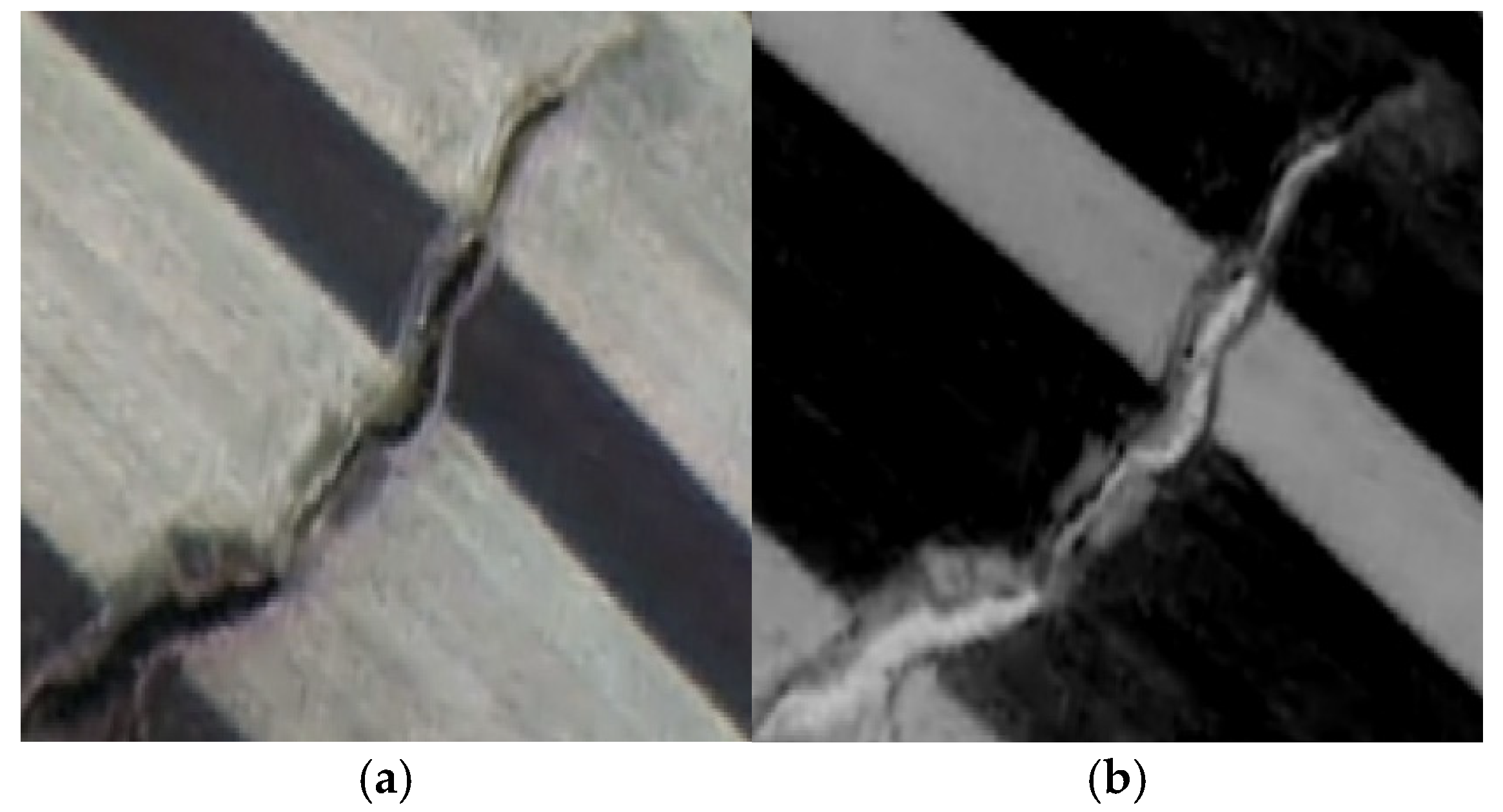
Figure 9 presents a comparison of gully representation in the same area using traditional high-resolution imagery and texture-enhanced composite imagery. In the traditional imagery (Figure 9a), gullies gradually merge into surrounding farmland, with indistinct boundaries that introduce substantial errors in manual crest-line annotation and hinder precise delineation of target margins. Such ambiguity reduces annotation accuracy and constrains the capacity of deep learning models to effectively capture the characteristics of linear landforms.
In contrast, the texture-enhanced composite imagery (Figure 9b), incorporating GLCM parameters such as contrast and mean, significantly amplifies the gray-level differences between gullies and adjacent features, producing clearer and more distinguishable boundary contours. Texture enhancement improves the morphological consistency and spatial continuity of linear gullies, thereby enabling the model to more accurately identify their orientation and width.
This comparative analysis demonstrates that texture-enhanced composite imagery enhances both the reliability and accuracy of manual annotations, while simultaneously providing a more discriminative data foundation prior to model training. These improvements establish a crucial basis for subsequent gains in extraction accuracy.

3.3. Comparison Between Multiple CNNs Based on Original Imagery

This study employs three CNNs—DeepLabv3+, U-Net, and U-Net++—to conduct segmentation training and testing on original remote sensing imagery, assessing their performance under varying conditions. Model performance was quantitatively evaluated using Acc, AP, IoU and Loss as metrics, with detailed results presented in Table 4.
As shown in Table 4, the comparative evaluation of U-Net, DeepLabv3+, and U-Net++ for erosion gully extraction from high-resolution remote sensing imagery demonstrates that U-Net achieved the best overall performance across all metrics. Specifically, U-Net yielded the highest accuracy (88.73%), which is 3.79% and 12.81% higher than those of DeepLabv3+ and U-Net++, respectively. In terms of average precision (AP), U-Net also surpassed the other two models, exceeding DeepLabv3+ by 2.55% and U-Net++ by 12.61%.
Furthermore, U-Net achieved the highest Intersection over Union (IoU) value of 82.50%, outperforming DeepLabv3+ (78.25%) and U-Net++ (68.75%). This superior IoU value indicates that U-Net not only provides more accurate pixel-level predictions but also ensures greater spatial consistency and overlap with reference gully areas. The improved IoU value underscores the model’s capability to precisely delineate erosion gully boundaries and maintain structural integrity during segmentation. U-Net obtained the lowest loss value (0.014), compared with 0.020 for DeepLabv3+ and 0.033 for U-Net++, highlighting its enhanced training stability and convergence efficiency. Collectively, these results suggest that U-Net not only achieves high accuracy in erosion gully identification but also effectively suppresses false detections, reflecting superior discriminative power and generalization capability.
Although DeepLabv3+ performed slightly below U-Net in terms of Acc, AP, and IoU, it still exhibited strong gully recognition ability, with an Acc of 84.94% and an IoU of 78.25%, outperforming U-Net++ across all metrics. In contrast, U-Net++ showed the weakest performance, characterized by the lowest Acc, AP, and IoU values and the highest training error. This finding suggests that U-Net++ has difficulty in capturing fine textures and boundary information in high-resolution imagery, rendering it less effective for erosion gully segmentation in this study.
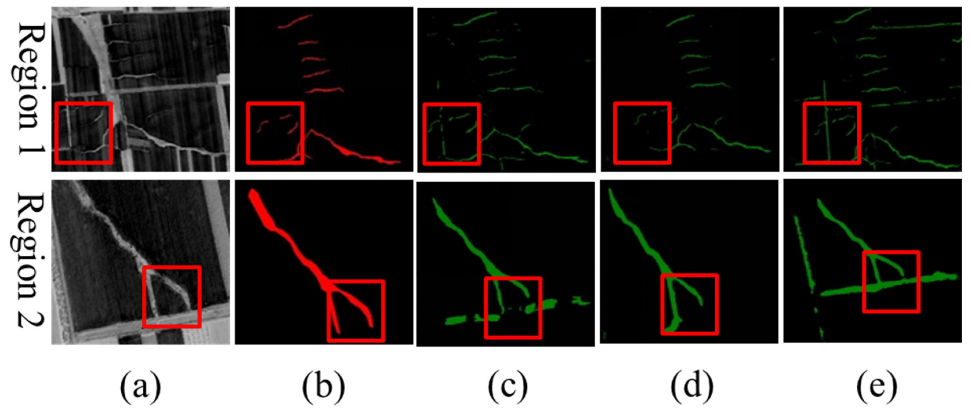
Figure 10 presents the extraction results of erosion gullies using the three CNN models (DeepLabv3+, U-Net, and U-Net++) under traditional high-resolution remote sensing imagery. Comparison with manual interpretation allows intuitive evaluation of differences in target recognition, boundary localization, and false extraction control among the models.
As shown in Figure 10c, DeepLabv3+ effectively captures the overall morphology of the main gullies, demonstrating strong global perceptual capability. However, its performance declines at detailed boundaries. In region 1 (red box), significant false extractions occur, with features such as field roads misclassified as gullies. This highlights the model’s limited ability to distinguish linear features within complex backgrounds.
The U-Net model, shown in Figure 10d, performs the best. It accurately restores the spatial morphology of gullies across multiple areas, with results highly consistent with manual interpretation. In region 2 (red box), U-Net successfully avoids interference from non-target features, producing clear boundaries and complete gully shapes. This superior performance is largely attributed to its skip connection mechanism, which enhances the fusion of low-level detail features and supports fine-grained target recognition.
By contrast, U-Net++ (Figure 10e) shows the weakest performance. Despite its theoretical advantage in multi-scale feature aggregation, the model produces numerous false positives and negatives. In region 2, large areas of farmland and roads are misclassified as gullies, with boundaries appearing blurred and incomplete. These errors reflect an overfitting tendency and poor adaptability to fine linear targets in high-resolution imagery.
Overall, U-Net not only achieves the highest quantitative accuracy under traditional imagery but also demonstrates superior visual performance. Its results confirm strong capability in preserving spatial structure and recognizing boundaries, underscoring its robustness, generalization ability, and application potential for gully extraction.

3.4. Comparison Between Multiple CNNs Based on Texture-Enhanced Composite Imagery

The same three CNNs and metrics were also used to verify the effectiveness of texture feature composite imagery for gully extraction. The results are summarized in Table 5.
As shown in Table 5, when using texture feature composite imagery, the U-Net model achieves the best overall performance across all evaluation metrics. Its Acc reaches 90.27%, which is 6.06% higher than DeepLabv3+ and 9.33% higher than U-Net++. The AP is 90.87%, exceeding DeepLabv3+ by 2.91% and U-Net++ by 6.42%. The IoU is 84.16%, surpassing DeepLabv3+ by 4.84% and U-Net++ by 10.66%. In terms of Loss, U-Net records the lowest value (0.011), reducing error by 0.014 compared with DeepLabv3+ (0.025) and by 0.015 compared with U-Net++ (0.026). These results demonstrate that U-Net not only provides the highest segmentation accuracy and intersection-over-union overlap but also offers greater training stability and stronger error control.
DeepLabv3+ ranks second, with an Acc of 84.21%, slightly lower than U-Net but 3.27% higher than U-Net++. Its AP is 87.96%, also below U-Net but above U-Net++ by 3.51%. The IoU is 79.32%, lower than U-Net but higher than U-Net++ by 5.82%. The Loss value of 0.025 is higher than U-Net’s but lower than U-Net++’s, indicating more reliable training performance. Overall, DeepLabv3+ shows strong extraction ability with texture feature composite imagery, maintains robustness in complex backgrounds, and achieves moderate boundary alignment as reflected by its IoU.
In contrast, U-Net++ performs the weakest, with an Acc of 80.94%, AP of 84.45%, IoU of 73.50%, and Loss of 0.026—the poorest results among the three models for all metrics. These findings indicate that U-Net++ has a higher error rate, lower extraction accuracy, and struggle to adapt effectively to the complex texture characteristics of erosion gullies in high-resolution remote sensing imagery.
To further validate these findings, typical regions identical to those used in the previous section were selected for visual comparison. The extraction results of DeepLabv3+, U-Net, and U-Net++ under texture feature composite imagery were examined to reveal practical differences among the models in spatial distribution, boundary recognition, and other aspects. To further validate these findings, typical regions identical to those used in the previous section were selected for visual comparison. The extraction results of DeepLabv3+, U-Net, and U-Net++ under texture feature composite imagery were examined to reveal practical differences among the models in spatial distribution, boundary recognition, and other aspects.
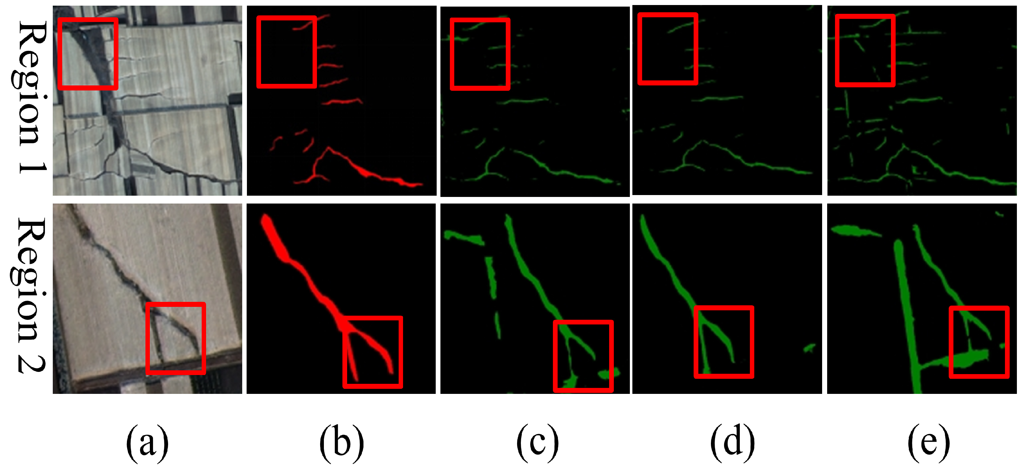
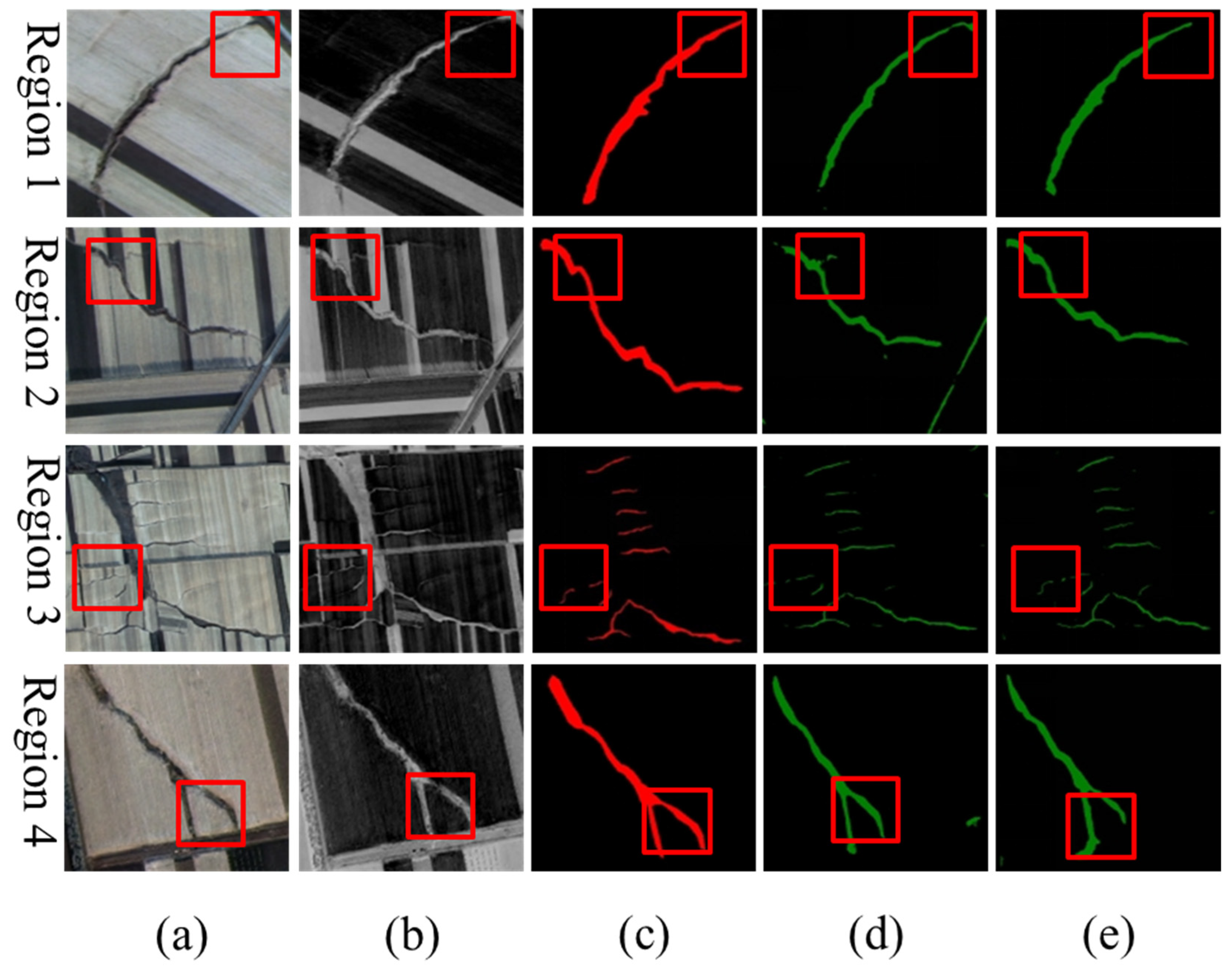
Figure 11 presents the extraction performance of the three models on texture feature composite images, with visual comparisons against manual interpretation to further assess the contribution of texture information to model performance.
In Figure 11d, the U-Net model continues to perform exceptionally well under texture enhancement, accurately delineating gully boundaries while preserving morphological continuity and detail. In the highlighted regions (region 1 and region 2), U-Net effectively suppresses interference from background features, avoiding the misclassification of similar linear structures such as field roads and farmland boundaries. The extraction results are highly consistent with manual interpretation. Heatmap analysis indicates that these improvements stem from the inclusion of texture features, which enhance the boundary contrast between gullies and surrounding areas.
The DeepLabv3+ model (Figure 11c) also shows improved results with texture-enhanced input. Compared with traditional imagery, false extractions are reduced and boundary clarity is moderately enhanced. However, in certain areas such as region 1, roads are still misclassified as gullies. This suggests that while DeepLabv3+ benefits from multi-scale recognition capabilities, it remains less effective than U-Net in preserving fine detail.
By contrast, U-Net++ (Figure 11e) shows only slight improvement relative to its performance on traditional imagery. Overall accuracy remains low, with evident false extractions and spurious responses in the red box areas, particularly along field boundaries and irrigation channels. These errors indicate that the model’s feature fusion strategy is less effective for this task, limiting its ability to discriminate between target and non-target features.
Overall, U-Net demonstrates the strongest performance under texture feature-enhanced conditions. Its extraction results not only align more closely with actual gully morphology but also achieve clearer boundaries and more complete target representation, confirming its adaptability and robustness in small-scale linear landform recognition.

3.5. Comparison Between Results Based on Different Inputs

Research results indicate that the U-Net++ model performs better in erosion gully extraction when using texture feature composite images compared with traditional high-resolution imagery, suggesting that the incorporation of texture features enhances its recognition capability to some extent. Nonetheless, its overall performance remains inferior to that of DeepLabv3+ and U-Net. In contrast, DeepLabv3+ demonstrates stronger extraction ability with traditional high-resolution imagery, but its performance declines slightly when texture features are introduced. The U-Net model consistently achieves the best results under both data source conditions, surpassing the other models in accuracy and stability, and showing strong adaptability and generalization.
Based on these findings, this study will further investigate the differential performance of the U-Net model in erosion gully extraction under varying data sources. The analysis will focus on extraction details in complex terrain, boundary recognition accuracy, and morphological restoration capacity, with the aim of comprehensively evaluating the practical enhancement effect of texture features on extraction accuracy.
Figure 12 compares the extraction results of the U-Net model under two data source conditions—traditional high-resolution images and texture feature composite images—using the same regions for visual analysis to further assess the role of texture features in improving recognition accuracy.
In regions 1 and 3, the results from traditional imagery (Figure 12d) reveal instances of false extraction, such as the misclassification of field roads and plot boundaries as gullies. Gully edges appear blurred, and morphological representation is incomplete. By contrast, with texture feature composite imagery (Figure 12e), U-Net effectively suppresses non-target responses, producing sharp boundaries, continuous structures, and overall contours that align more closely with manual interpretation.
The comparison in region 2 highlights the contribution of texture features to detail retention. In Figure 12e, U-Net not only delineates the main gully but also captures smaller secondary gullies, displaying natural orientations and smooth contours. This performance is markedly superior to the fragmented extraction observed in Figure 12d. Although false extractions are still present in region 4, the non-target responses are significantly reduced under the texture feature condition, further confirming the model’s improved boundary discrimination.
Overall, the incorporation of texture features substantially enhances U-Net’s extraction accuracy, boundary recognition, and preservation of gully structural integrity. In particular, the model demonstrates a stronger ability to distinguish erosion gullies from spectrally or morphologically similar features in complex backgrounds, underscoring the critical role of texture information in guiding the learning of key edge and morphological characteristics.

3.6. Analysis of Class Activation Maps and Error

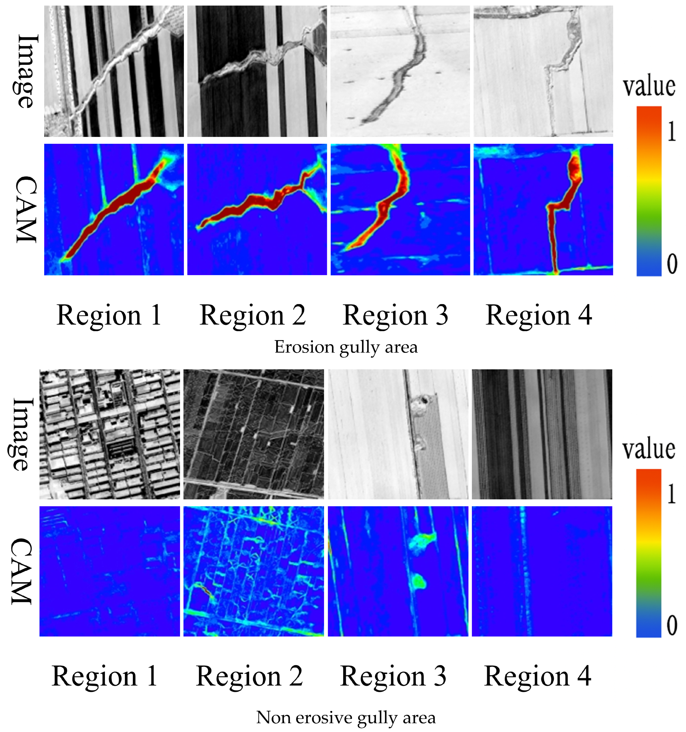
To further investigate the regions emphasized by the model during erosion gully recognition and to identify potential error sources, this study applies CAM for visual analysis of the U-Net model. By combining convolutional feature maps with the corresponding class weights, a spatial response heatmap of the erosion gully category is generated, revealing both the model’s discriminative basis and its spatial attention distribution.
Figure 13 illustrates the activation distribution for correctly recognized samples. The heatmap shows strong responses within erosion gully areas (dense red regions), with intensity gradually weakening from the center outward. This indicates that the model accurately attends to gullies and effectively captures their linear morphological features. In contrast, non-gully areas such as farmland, forest land, and residential zones exhibit low overall heat intensity, suggesting clear class boundaries and good target discrimination ability.
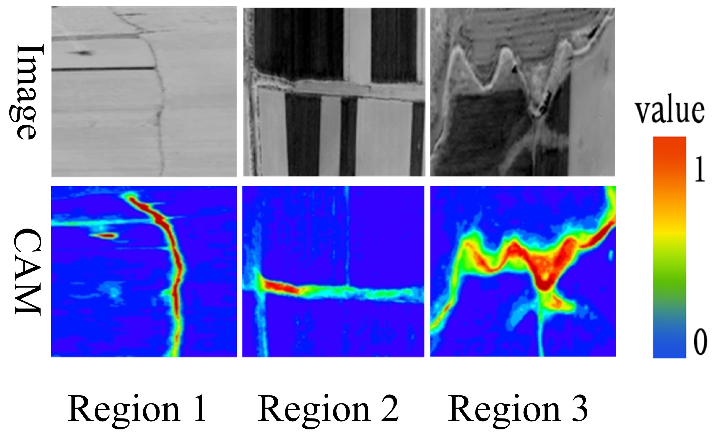
However, Figure 14 highlights cases of false extraction, mainly concentrated on linear features such as field roads, farmland edges, irrigation channels, and small tributaries. These features share strong similarities with gullies in terms of texture, grayscale, and morphology, which can trigger false positive responses. The corresponding heatmaps display high activation in these non-target regions, demonstrating that the model’s recognition mechanism remains susceptible to confusion under such interference.
Overall, CAM analysis confirms that the model successfully extracts erosion gully areas in most cases but still struggles to differentiate gullies from morphologically or texturally similar background features. To mitigate this limitation, future work could integrate attention mechanisms, graph-based modeling, and prior boundary constraints to enhance recognition stability and improve semantic differentiation in complex environments.

4. Discussion

4.1. Research Overview and Key Findings

This study proposes an automatic extraction method that integrates high-resolution remote sensing imagery, texture features, and multiple CNN models to monitor erosion gullies in the thick black soil region of Northeast China. The results show that the U-Net model outperforms DeepLabv3+ and U-Net++ in both accuracy and precision, achieving improvements of 1.54% in Acc and 1.38% in AP after the integration of texture features. These findings underscore the potential of this method for large-scale agricultural gully monitoring.

4.2. Mechanisms of CNN Models for Erosion Gully Extraction

The superior performance of U-Net primarily stems from its symmetric encoder–decoder architecture and multi-level skip connections: during downsampling, the encoder progressively aggregates multi-scale contextual information, while skip connections enable precise alignment and fusion of shallow-layer features with deep semantic representations during upsampling, thereby substantially mitigating spatial detail loss induced by deep network stacking. This mechanism is particularly suited for identifying narrow linear features (e.g., gully edges and their continuity), as it preserves fine-grained spatial cues captured in shallow layers, which are prone to smoothing in purely semantics-driven deep representations. Under GLCM texture-enhanced inputs, these cross-layer fusion pathways further strengthen the injection of low-level grayscale and edge information into high-level semantics, thereby enhancing boundary discrimination accuracy and morphological continuity restoration; from a feature flow perspective, skip connections not only reduce information entropy loss during feature extraction but also heighten the model’s sensitivity to small-scale linear targets, aligning closely with the elongated and discontinuous characteristics of gullies in black soil regions and averting cumulative suppression of local details due to gradient vanishing in conventional downsampling paths.
U-Net++ incorporates dense skip connections and nested decoding structures to enhance feature representation, but its performance in this study was inferior to U-Net. Multi-level feature fusion under these data conditions may introduce redundancy, diluting or duplicating texture enhancement signals and reducing the recognition of detailed features. Moreover, U-Net++ is more sensitive to noise, particularly in the heterogeneous backgrounds of black soil regions, where deep connections may amplify non-target signals and lead to false extractions.
DeepLabv3+ outperforms U-Net++ on traditional images but shows a decline in Acc (84.94% → 84.21%) with texture-enhanced inputs, indicating limited adaptability to GLCM-derived local texture information. The main reason lies in DeepLabv3+’s weak local spatial dependency. Its backbone relies on dilated convolutions, which expand the receptive field to capture multi-scale contextual information. Although effective for large-scale structures, this approach is inherently limited in capturing fine boundaries and local texture variations. GLCM-extracted texture features exhibit distinct local statistical properties, with enhanced information concentrated on small-scale grayscale contrasts and edge directions, which are diluted by dilated convolutions as the receptive field expands. Furthermore, DeepLabv3+ lacks a fine-grained feature transfer mechanism such as U-Net’s skip connections, preventing effective integration of texture enhancement into the semantic decoding path and limiting boundary differentiation. This aligns with the visualization results in Figure 11c, where field roads are still misclassified as erosion gullies under texture input, indicating a limited response to boundary features introduced by GLCM.

4.3. Innovation of the GLCM-CNN Integration Method and Its Practical Application Value

The findings of this study align closely with recent advancements in CNN-based semantic segmentation for geomorphological feature extraction, particularly deep learning applications targeting erosion gullies in Northeast China’s black soil region [19,62]. From a regional perspective, this study focuses on the core thick black soil area in Northeast China, exhibiting high geographical consistency with gully susceptibility assessments in the same black soil region by Huang et al. (2023) [63] and Liu et al. (2024) [64]; however, the latter primarily rely on statistical modeling of topographic factors (e.g., slope, curvature, and flow accumulation) for susceptibility mapping, whereas this study achieves end-to-end automated semantic segmentation, markedly improving the precise geometric representation and continuity restoration of gully morphologies while avoiding common threshold dependencies and post-processing biases in susceptibility assessments. From an input perspective, this method innovatively incorporates contrast and mean texture features via GLCM band stacking, directly augmenting local second-order statistical information in high-resolution optical imagery and thereby effectively mitigating confusion among spectrally similar classes (e.g., field roads and gully edges); although Liu et al.’s (2024) [64] pure spectral multi-scale satellite imagery input enables efficient global context capture, it lacks explicit reinforcement of small-neighborhood grayscale contrasts and directional consistencies, resulting in limited boundary discrimination under black soil backgrounds with high inter-class spectral overlap. From a model perspective, the GLCM-fused U-Net leverages its inherent symmetric encoder–decoder and layer-aligned skip connection mechanisms to achieve precise fusion of shallow-layer texture cues with deep semantics, markedly outperforming the DD-DA DeepLabv3+ variant of Zhang et al. (2024) [19], which, despite incorporating dual-branch dynamic attention modules to bolster boundary responses, suffers from receptive field expansion dominated by dilated convolutions that readily dilutes GLCM-induced local texture details, resulting in insufficient detail injection in texture-enhanced scenarios; compared to Li et al.’s (2025) [62] Gully-ERFNet, which relies on efficient residual attention modules to compensate for the expressive capacity of its lightweight backbone, this study achieves more robust fine-grained linear feature restoration via input-level texture augmentation without such architectural extensions—this advantage further underscores the potential efficacy of input representation optimization over purely architectural modifications, particularly in computationally constrained large-scale monitoring in black soil regions; overall, this study diverges from prior DEM-dependent approaches [63] or purely architecture-oriented studies (e.g., the multi-scale content-structure fusion network of Dong et al., 2024 [65]) by prioritizing texture fusion, thereby addressing a systematic gap in exploring the interplay between input representations and model adaptability in black soil gully extraction.
This method advances the theoretical application of texture feature fusion and demonstrates efficient large-scale gully extraction in practice, particularly for land management in Northeast China’s black soil region. When integrated into soil and water conservation monitoring platforms, this method enables real-time monitoring and provides an effective tool to support agricultural sustainability within the framework of the United Nations Sustainable Development Goals. Its efficiency reduces the need for extensive fieldwork, thereby lowering costs and improving monitoring accuracy.

4.4. Research Limitations and Future Directions

Although the proposed method demonstrates strong performance in the black soil region, its generalization ability remains constrained. Specifically, the dependence on high-resolution imagery limits its applicability to coarser-resolution datasets, such as Sentinel-2. The minimum detectable gully size is inherently restricted by the spatial resolution of the input imagery, which may lead to the omission of small or subtle gullies and consequently influence the accuracy of gully density and spatial pattern analyses.
Moreover, the method’s robustness is susceptible to data quality challenges, including cloud contamination, seasonal vegetation dynamics, and varying atmospheric conditions. These factors can degrade image clarity and consistency, thereby introducing uncertainties into both feature extraction and model prediction processes.
Additionally, the dataset employed in this study encompasses only the core black soil area, neglecting the topographic and land-use variability present in peripheral regions. The relatively limited sample size (1175/1141 samples) may constrain model generalization to rare gully morphologies. Future work should incorporate larger, more diverse datasets and explore active learning for efficient annotation expansion to enhance model robustness and transferability through the integration of multi-source data fusion (e.g., combining optical and radar observations) and the development of preprocessing strategies to mitigate the effects of atmospheric and environmental disturbances.

5. Conclusions

This study proposed a texture-enhanced deep learning framework for automated gully extraction in the black soil region of Northeast China, addressing the persistent challenges of boundary ambiguity and spectral confusion in complex agricultural landscapes. Systematic optimization of GLCM parameters (5 × 5 window, 32 gray levels) enabled the fusion of mean and contrast texture features with high-resolution multispectral imagery, significantly improving gully delineation accuracy. Quantitatively, U-Net achieved an overall accuracy of 90.27%, an average precision of 90.87%, and an IoU of 84.16%, outperforming DeepLabv3+ and U-Net++ by 6.06% and 9.33%, respectively.
Methodologically, this work advances the field by establishing a reproducible workflow that integrates texture parameter optimization, multi-source fusion, and CAM-based interpretability analysis into a unified framework. Unlike prior studies focused solely on architectural innovation or DEM dependence, this approach emphasizes input-level representation optimization, demonstrating that enhancing local texture information can yield greater performance gains than complex architectural modifications. The interpretability analysis further revealed how texture fusion sharpens edge attention and mitigates false responses from spectrally similar features such as field roads and farmland boundaries, providing mechanistic insights into model behavior.

Author Contributions

J.Y. (Jiaxin Yu): Writing—review and editing, Writing—original draft, Visualization, Validation, Software, Resources, Methodology, Investigation, Formal analysis, Data curation, Conceptualization. J.Y. (Jiuchun Yang): Writing—review and editing, Supervision, Resources, Funding acquisition, Conceptualization. X.X.: Software, Resources, Methodology, Investigation, Visualization, Data curation. L.K.: Software. All authors have read and agreed to the published version of the manuscript.

Funding

This study was supported by the Strategic Priority Research Program of the Chinese Academy of Sciences (Grant No. XDA28070502), the National Natural Science Foundation of China (Grant No. 42171380), and the National Key RD Program of China (Grant No. 2021YFD1500102). The APC was funded by the corresponding author.

Data Availability Statement

The raw data supporting the conclusions of this article will be made available by the authors on request.

Acknowledgments

We gratefully acknowledge the Satellite Application Center for Ecology and Environment, Ministry of Ecology and Environment for generously providing the essential satellite data used in this study. We also thank the editors and anonymous reviewers for their enthusiastic, patient, and constructive comments that significantly improved the quality of this manuscript.

Conflicts of Interest

The authors declare that they have no known competing financial interest or personal relationships that could have appeared to influence the work reported in this paper.

References

  1. Li, Y.; Wang, L.; Yu, Y.; Zang, D.; Dai, X.; Zheng, S. Cropland zoning based on district and county scales in the black soil region of northeastern China. Sustainability 2024, 16, 3341. [Google Scholar] [CrossRef]
  2. He, J.; Ran, D.; Tan, D.; Liao, X. Spatiotemporal evolution of cropland in Northeast China’s black soil region over the past 40 years at the county scale. Front. Sustain. Food Syst. 2024, 7, 1332595. [Google Scholar] [CrossRef]
  3. Wang, R.; Sun, H.; Yang, J.; Zhang, S.; Fu, H.; Wang, N.; Liu, Q. Quantitative evaluation of gully erosion using multitemporal UAV data in the southern black soil region of Northeast China: A case study. Remote Sens. 2022, 14, 1479. [Google Scholar] [CrossRef]
  4. Gao, P.; Li, Z.; Liu, X.; Zhang, S.; Wang, Y.; Liang, A.; Zhang, Y.; Wen, X.; Hu, W.; Zhou, Y. Temporal and spatial distribution and development of permanent gully in cropland in the rolling hill region (phaeozems area) of northeast China. Catena 2024, 235, 107625. [Google Scholar] [CrossRef]
  5. Dong, Y.; Wu, Y.; Qin, W.; Guo, Q.; Yin, Z.; Duan, X. The gully erosion rates in the black soil region of northeastern China: Induced by different processes and indicated by different indexes. Catena 2019, 182, 104146. [Google Scholar] [CrossRef]
  6. Kinsey-Henderson, A.; Hawdon, A.; Bartley, R.; Wilkinson, S.N.; Lowe, T. Applying a hand-held laser scanner to monitoring gully erosion: Workflow and evaluation. Remote Sens. 2021, 13, 4004. [Google Scholar] [CrossRef]
  7. Wang, J.; Yang, J.; Li, Z.; Ke, L.; Li, Q.; Fan, J.; Wang, X. Research on soil erosion based on remote sensing technology: A review. Agriculture 2025, 15, 18. [Google Scholar] [CrossRef]
  8. Lu, P.; Zhang, B.; Wang, C.; Liu, M.; Wang, X. Erosion gully networks extraction based on InSAR refined digital elevation model and relative elevation algorithm—A case study in Huangfuchuan Basin, Northern Loess Plateau, China. Remote Sens. 2024, 16, 921. [Google Scholar] [CrossRef]
  9. Zhang, C.; Wang, C.; Long, Y.; Pang, G.; Shen, H.; Wang, L.; Yang, Q. Comparative analysis of gully morphology extraction suitability using unmanned aerial vehicle and Google Earth imagery. Remote Sens. 2023, 15, 4302. [Google Scholar] [CrossRef]
  10. Wang, L.; Wang, J.; Zhang, X.; Wang, L.; Qin, F. Deep segmentation and classification of complex crops using multi-feature satellite imagery. Comput. Electron. Agric. 2022, 200, 107249. [Google Scholar] [CrossRef]
  11. Slimane, A.B.; Raclot, D.; Rebai, H.; Le Bissonnais, Y.; Planchon, O.; Bouksila, F. Combining field monitoring and aerial imagery to evaluate the role of gully erosion in a Mediterranean catchment (Tunisia). Catena 2018, 170, 73–83. [Google Scholar] [CrossRef]
  12. Shahabi, H.; Jarihani, B.; Tavakkoli Piralilou, S.; Chittleborough, D.; Avand, M.; Ghorbanzadeh, O. A semi-automated object-based gully networks detection using different machine learning models: A case study of Bowen Catchment, Queensland, Australia. Sensors 2019, 19, 4893. [Google Scholar] [CrossRef]
  13. Chen, Z.; Liu, T. Verifying the effects of the grey level co-occurrence matrix and topographic–hydrologic features on automatic gully extraction in Dexiang Town, Bayan County, China. Remote Sens. 2025, 17, 2563. [Google Scholar] [CrossRef]
  14. Lan, Z.; Liu, Y. Study on multi-scale window determination for GLCM texture description in high-resolution remote sensing image geo-analysis supported by GIS and domain knowledge. ISPRS Int. J. Geo-Inf. 2018, 7, 175. [Google Scholar] [CrossRef]
  15. Moya, L.; Zakeri, H.; Yamazaki, F.; Liu, W.; Mas, E.; Koshimura, S. 3D gray level co-occurrence matrix and its application to identifying collapsed buildings. ISPRS J. Photogramm. Remote Sens. 2019, 149, 14–28. [Google Scholar] [CrossRef]
  16. Alam, M.; Wang, J.F.; Guangpei, C.; Yunrong, L.V.; Chen, Y. Convolu-tional neural network for the semantic segmentation of remote sensing images. Mob. Netw. Appl. 2021, 26, 200–215. [Google Scholar] [CrossRef]
  17. Chen, X.; Li, D.; Liu, M.; Jia, J. CNN and transformer fusion for remote sensing image semantic segmentation. Remote Sens. 2023, 15, 4455. [Google Scholar] [CrossRef]
  18. Wang, H.; Miao, F. Building extraction from remote sensing images using deep residual U-Net. Eur. J. Remote Sens. 2022, 55, 71–85. [Google Scholar] [CrossRef]
  19. Zhang, X.; Zhang, S.; Meng, X.; Zhang, G.; Zang, D.; Han, Y.; Ai, H.; Liu, H. Remote sensing image segmentation of gully erosion in a typical black soil area in Northeast China based on improved DeepLabV3+ model. Ecol. Inform. 2024, 84, 102929. [Google Scholar] [CrossRef]
  20. Chen, L.C.; Zhu, Y.; Papandreou, G.; Schroff, F.; Adam, H. Encoder-decoder with atrous separable convolution for semantic image segmentation. In Proceedings of the European Conference on Computer Vision (ECCV), Munich, Germany, 8–14 September 2018; Springer: Berlin/Heidelberg, Germany, 2018; pp. 801–818. [Google Scholar] [CrossRef]
  21. Diakogiannis, F.I.; Waldner, F.; Caccetta, P.; Wu, C. ResUNet-a: A deep learning framework for semantic segmentation of remotely sensed data. ISPRS J. Photogramm. Remote Sens. 2020, 162, 94–114. [Google Scholar] [CrossRef]
  22. Li, X.; Li, Y.; Ai, J.; Shu, Z.; Xia, J.; Xia, Y. Semantic segmentation of UAV remote sensing images based on edge feature fusing and multi-level upsampling integrated with Deeplabv3+. PLoS ONE 2023, 18, e0279097. [Google Scholar] [CrossRef]
  23. Chen, Z.; Wang, C.; Li, J.; Fan, W.; Du, J.; Zhong, B. Adaboost-like end-to-end multiple lightweight U-Nets for road extraction from optical remote sensing images. Int. J. Appl. Earth Obs. Geoinf. 2021, 100, 102341. [Google Scholar] [CrossRef]
  24. Zhao, J.; Ma, T.; Wang, Z.; Cachim, P.; Qin, M. Pavement crack detection and segmentation using nested U-Net with residual attention mechanism. Comput.-Aided Civ. Infrastruct. Eng. 2025, 40, 4076–4092. [Google Scholar] [CrossRef]
  25. Li, H.; Jin, J.; Dong, F.; Zhang, J.; Li, L.; Zhang, Y. Gully erosion susceptibility prediction using high-resolution data: Evaluation, comparison, and improvement of multiple machine learning models. Remote Sens. 2024, 16, 4742. [Google Scholar] [CrossRef]
  26. Javidan, N.; Kavian, A.; Conoscenti, C.; Jafarian, Z.; Kalehhouei, M.; Javidan, R. Development of risk maps for flood, landslide, and soil erosion using machine learning model. Nat. Hazards 2024, 120, 11987–12010. [Google Scholar] [CrossRef]
  27. Lana, J.C.; Castro, P.D.T.A.; Lana, C.E. Assessing gully erosion susceptibility and its conditioning factors in southeastern Brazil using machine learning algorithms and bivariate statistical methods: A regional approach. Geomorphology 2022, 402, 108159. [Google Scholar] [CrossRef]
  28. Thanh, B.N.; Van Phong, T.; Trinh, P.T.; Costache, R.; Amiri, M.; Nguyen, D.D.; Van Le, H.; Prakash, I.; Pham, B.T. Prediction of coastal erosion susceptible areas of Quang Nam Province, Vietnam using machine learning models. Earth Sci. Inform. 2024, 17, 401–419. [Google Scholar] [CrossRef]
  29. Phinzi, K.; Ngetar, N.S.; Le Roux, J.J. Predictive machine learning for gully susceptibility modeling with geo-environmental covariates: Main drivers, model performance, and computational efficiency. Nat. Hazards 2024, 120, 8239–8272. [Google Scholar] [CrossRef]
  30. Alkahtani, M.; Mallick, J.; Alqadhi, S.; Sarif, M.N.; Fatahalla Mohamed Ahmed, M.; Abdo, H.G. Interpretation of Bayesian-optimized deep learning models for enhancing soil erosion susceptibility prediction and management: A case study of Eastern India. Geocarto Int. 2024, 39, 2367611. [Google Scholar] [CrossRef]
  31. Bi, Q.; Qin, K.; Li, Z.; Zhang, H.; Xu, K.; Xia, G.S. A multiple-instance densely-connected ConvNet for aerial scene classification. IEEE Trans. Image Process. 2021, 29, 4911–4926. [Google Scholar] [CrossRef]
  32. Yang, G.; Zhang, Q.; Zhang, G. EANet: Edge-aware network for the extraction of buildings from aerial images. Remote Sens. 2020, 12, 2161. [Google Scholar] [CrossRef]
  33. Liu, X.B.; Zhang, X.Y.; Wang, Y.X.; Sui, Y.Y.; Zhang, S.L.; Herbert, S.J.; Ding, G. Soil degradation: A problem threatening the sustainable development of agriculture in Northeast China. Plant Soil Environ. 2010, 56, 87–97. [Google Scholar] [CrossRef]
  34. Gao, Q.; Ma, L.; Fang, Y.; Zhang, A.; Li, G.; Wang, J.; Wu, D.; Wu, W.; Du, Z. Conservation tillage for 17 years alters the molecular composition of organic matter in soil profile. Sci. Total Environ. 2021, 762, 143116. [Google Scholar] [CrossRef] [PubMed]
  35. Liu, X.; Li, H.; Zhang, S.; Cruse, R.M.; Zhang, X. Gully erosion control practices in Northeast China: A review. Sustainability 2019, 11, 5065. [Google Scholar] [CrossRef]
  36. Bharati, M.H.; Liu, J.J.; MacGregor, J.F. Image texture analysis: Methods and comparisons. Chemom. Intell. Lab. Syst. 2004, 72, 57–71. [Google Scholar] [CrossRef]
  37. Bianconi, F.; Fernández, A.; Smeraldi, F.; Pascoletti, G. Colour and texture descriptors for visual recognition: A historical overview. J. Imaging 2021, 7, 245. [Google Scholar] [CrossRef]
  38. Alçin Ö, F.; Siuly, S.; Bajaj, V.; Guo, Y.; Şengu, A.; Zhang, Y. Multi-category EEG signal classification developing time-frequency texture features based Fisher Vector encoding method. Neurocomputing 2016, 218, 251–258. [Google Scholar] [CrossRef]
  39. Zhang, X.; Cui, J.; Wang, W.; Lin, C. A study for texture feature extraction of high-resolution satellite images based on a direction measure and gray level co-occurrence matrix fusion algorithm. Sensors 2017, 17, 1474. [Google Scholar] [CrossRef]
  40. Sill, M.; Saadati, M.; Benner, A. Applying stability selection to consistently estimate sparse principal components in high-dimensional molecular data. Bioinformatics 2015, 31, 2683–2690. [Google Scholar] [CrossRef]
  41. Huang, P.; Ye, Q.; Zhang, F.; Yang, G.; Zhu, W.; Yang, Z. Double L 2, p-norm based PCA for feature extraction. Inf. Sci. 2021, 573, 345–359. [Google Scholar] [CrossRef]
  42. Nwokoma, F.; Foreman, J.; Akujuobi, C.M. Effective data reduction using discriminative feature selection based on principal component analysis. Mach. Learn. Knowl. Extr. 2024, 6, 789–799. [Google Scholar] [CrossRef]
  43. Hall-Beyer, M. Practical guidelines for choosing GLCM textures to use in landscape classification tasks over a range of moderate spatial scales. Int. J. Remote Sens. 2017, 38, 1312–1338. [Google Scholar] [CrossRef]
  44. Liu, J.; Zhu, Y.; Song, L.; Su, X.; Li, J.; Zheng, J.; Zhu, X.; Ren, L.; Wang, W.; Li, X. Optimizing window size and directional parameters of GLCM texture features for estimating rice AGB based on UAVs multispectral imagery. Front. Plant Sci. 2023, 14, 1284235. [Google Scholar] [CrossRef] [PubMed]
  45. Brynjolfsson, P.; Nilsson, D.; Torheim, T.; Asklund, T.; Karlsson, C.T.; Trygg, J.; Nyholm, T.; Garpebring, A. Haralick texture features from apparent diffusion coefficient (ADC) MRI images depend on imaging and pre-processing parameters. Sci. Rep. 2017, 7, 4042. [Google Scholar] [CrossRef]
  46. Clausi, D.A. An analysis of co-occurrence texture statistics as a function of grey level quantization. Can. J. Remote Sens. 2002, 28, 45–62. [Google Scholar] [CrossRef]
  47. Murray, H.; Lucieer, A.; Williams, R. Texture-based classification of sub- Antarctic vegetation communities on Heard Island. Int. J. Appl. Earth Obs. Geoinf. 2010, 12, 138–149. [Google Scholar] [CrossRef]
  48. Balling, J.; Reiche, J.; Herold, M. How textural features can improve SAR-based tropical forest disturbance mapping. Int. J. Appl. Earth Obs. Geoinf. 2023, 122, 103492. [Google Scholar] [CrossRef]
  49. Shuvo, M.B.; Ahommed, R.; Reza, S.; Hashem, M.M.A. CNL-UNet: A novel lightweight deep learning architecture for multimodal biomedical image segmentation with false output suppression. Biomed. Signal Process. Control. 2021, 70, 102959. [Google Scholar] [CrossRef]
  50. Xiang, T.; Zhang, C.; Wang, X.; Song, Y.; Liu, D.; Huang, H.; Cai, W. Towards bi-directional skip connections in encoder-decoder architectures and beyond. Med. Image Anal. 2022, 78, 102420. [Google Scholar] [CrossRef]
  51. Shi, P.; Duan, M.; Yang, L.; Feng, W.; Ding, L.; Jiang, L. An improved U-Net image segmentation method and its application for metallic grain size statistics. Materials 2022, 15, 4417. [Google Scholar] [CrossRef]
  52. Ronneberger, O.; Fischer, P.; Brox, T. U-Net: Convolutional networks for biomedical image segmentation. In Proceedings of the Medical Image Computing and Computer-Assisted Intervention—MICCAI 2015, Munich, Germany, 5–9 October 2015; Springer: Berlin/Heidelberg, Germany, 2015; pp. 234–241. [Google Scholar] [CrossRef]
  53. Zhou, Z.; Rahman Siddiquee, M.M.; Tajbakhsh, N.; Liang, J. UNet++: A nested U-Net architecture for medical image segmentation. In Deep Learning in Medical Image Analysis and Multimodal Learning for Clinical Decision Support; Springer: Cham, Switzerland, 2019; pp. 3–11. [Google Scholar] [CrossRef]
  54. Liu, Y.; Bai, X.; Wang, J.; Li, G.; Li, J.; Lv, Z. Image semantic segmentation approach based on DeepLabV3 plus network with an attention mechanism. Eng. Appl. Artif. Intell. 2024, 127, 107260. [Google Scholar] [CrossRef]
  55. Wang, Y.; Gao, X.; Sun, Y.; Liu, Y.; Wang, L.; Liu, M. Sh-DeepLabv3+: An improved semantic segmentation lightweight network for corn straw cover form plot classification. Agriculture 2024, 14, 628. [Google Scholar] [CrossRef]
  56. Guo, X. Research on Iris Segmentation Method Based on Improved DeepLab-V3+ Structure. Master’s Thesis, Jilin University, Changchun, China, 2024. [Google Scholar] [CrossRef]
  57. Goodfellow, I.; Bengio, Y.; Courville, A. Deep Learning; MIT Press: Cambridge, MA, USA, 2016. [Google Scholar] [CrossRef]
  58. Zhou, B.; Khosla, A.; Lapedriza, A.; Oliva, A.; Torralba, A. Learning deep features for discriminative localization. In Proceedings of the IEEE Conference on Computer Vision and Pattern Recognition, Las Vegas, NV, USA, 27–30 June 2016; pp. 2921–2929. [Google Scholar] [CrossRef]
  59. Feng, Z.; Zhu, M.; Stanković, L.; Ji, H. Self-matching CAM: A novel accurate visual explanation of CNNs for SAR image interpretation. Remote Sens. 2021, 13, 1772. [Google Scholar] [CrossRef]
  60. Patel, M.B.; Rodriguez, J.J.; Gmitro, A.F. Effect of gray-level re-quantization on co-occurrence based texture analysis. In Proceedings of the 2008 15th IEEE International Conference on Image Processing, San Diego, CA, USA, 12–15 October 2008; pp. 585–588. [Google Scholar] [CrossRef]
  61. Wang, Y.; Gu, M. Classification methods for hyperspectral remote sensing images with weak texture features. J. Radiat. Res. Appl. Sci. 2024, 17, 101019. [Google Scholar] [CrossRef]
  62. Li, Q.; Yang, J.; Wang, J.; Li, Z.; Fan, J.; Ke, L.; Wang, X. Gully-ERFNet: A novel lightweight deep learning model for extracting erosion gullies in the black soil region of Northeast China. Int. J. Digit. Earth 2025, 18, 2494074. [Google Scholar] [CrossRef]
  63. Huang, D.; Su, L.; Zhou, L.; Tian, Y.; Fan, H. Assessment of gully erosion susceptibility using different DEM-derived topographic factors in the black soil region of Northeast China. Int. Soil Water Conserv. Res. 2023, 11, 97–111. [Google Scholar] [CrossRef]
  64. Liu, C.; Fan, H.; Wang, Y. Gully erosion susceptibility assessment using three machine learning models in the black soil region of Northeast China. Catena 2024, 245, 108275. [Google Scholar] [CrossRef]
  65. Dong, F.; Jin, J.; Li, L.; Li, H.; Zhang, Y. A Multi-Scale Content-Structure Feature Extraction Network Applied to Gully Extraction. Remote Sens. 2024, 16, 3562. [Google Scholar] [CrossRef]
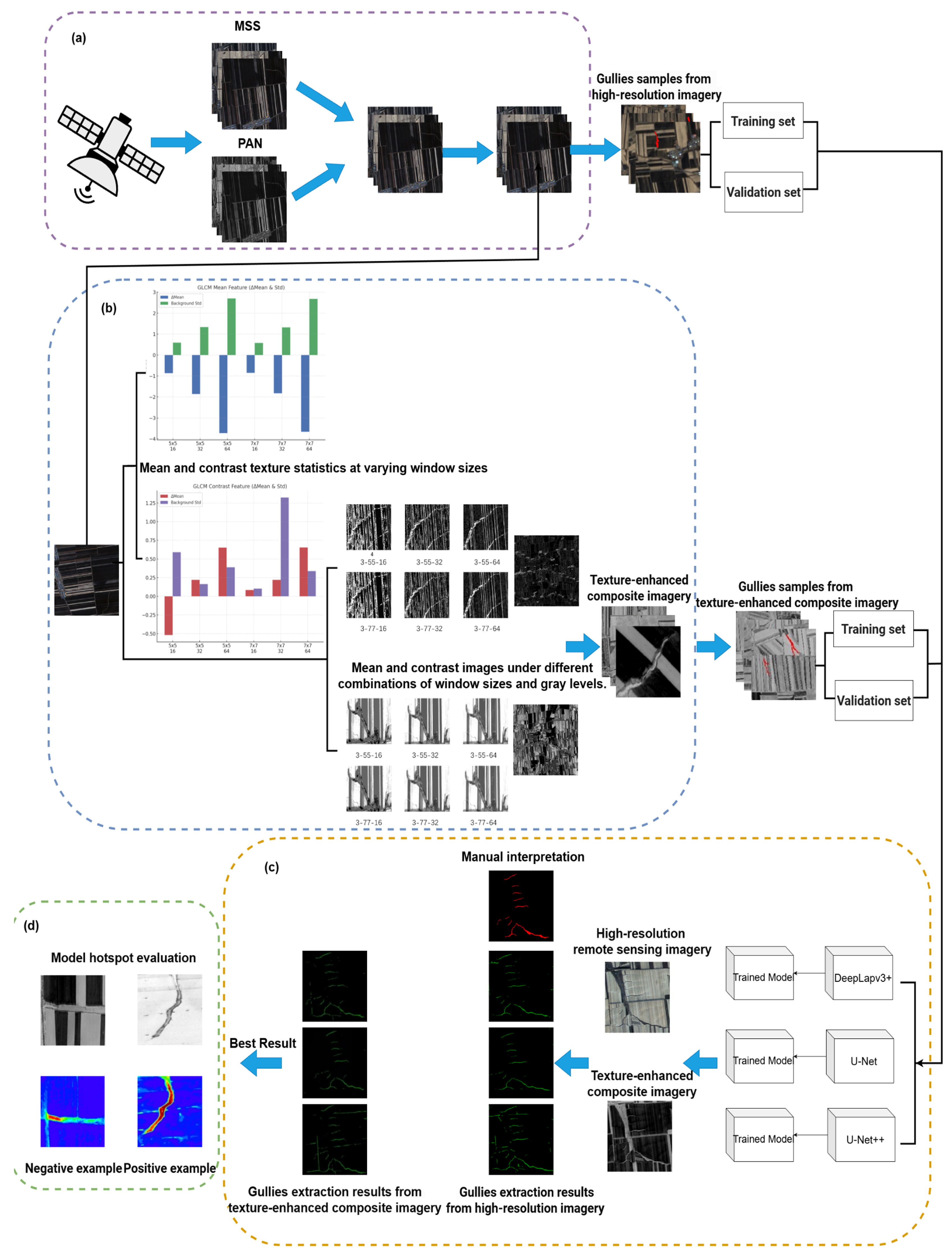
Figure 1. Technical roadmap of the proposed framework. (a) Preprocessing of remote sensing imagery. (b) GLCM-based texture feature extraction and fusion to generate composite images. (c) Training and evaluation of CNN models. (d) CAM visualization for identifying regions of model focus.
Remotesensing 17 03792 g001
Figure 2. Location of the study area. Administrative boundaries in the figure are drawn based on publicly available map data.
Remotesensing 17 03792 g002
Figure 3. Schematic diagrams of the cross-sectional and planform morphology of a typical gully. (a) Vertical cross-sectional structure of the gully; (b) Planform morphology of the gully.
Remotesensing 17 03792 g003
Figure 5. Architecture of U-Net++ (redrawn from Zhou et al., 2019 [53]).(a) Original UNet++ with dense skip pathways (cyan) and deep supervision (red arrows). (b) Redesigned UNet++ using full-scale skip connections that aggregate features from all encoder levels. (c) Pruned UNet++ for inference, retaining only the final segmentation output L4 while removing intermediate supervision branches.
Remotesensing 17 03792 g005
Figure 6. DeepLabv3+ network architecture. (redrawn from Guo, 2024 [56]).
Remotesensing 17 03792 g006
Figure 7. GLCM texture images under different parameter combinations. (a) Contrast feature image; (b) Mean feature image.
Remotesensing 17 03792 g007
Figure 8. Comparison of GLCM texture feature images of Band 3 under different combinations of sliding windows and gray levels. (a) Contrast feature image; (b) Mean feature image.
Remotesensing 17 03792 g008
Figure 9. Comparison of image expression differences in erosion gully landforms under different data sources. (a) Traditional high-resolution remote sensing image; (b) Composite image fused with GLCM texture features.
Remotesensing 17 03792 g009
Figure 10. Comparison of erosion gully extraction results of three CNN models under traditional high-resolution remote sensing images. (a) Original image; (b) Manual interpretation results; (ce) Extraction results of DeepLabv3+, U-Net, and U-Net++, respectively. The red box areas are used to highlight the differences between models in boundary recognition and false extraction control.
Remotesensing 17 03792 g010
Figure 11. Comparison of erosion gully extraction results of three CNN models under texture feature combined image input conditions. (a) Original image; (b) Manual interpretation results; (ce) Segmentation results of DeepLabv3+, U-Net, and U-Net++ models, respectively. The red box areas are used to highlight the differences between models in boundary recognition and false extraction control.
Remotesensing 17 03792 g011
Figure 12. Comparison of U-Net model erosion gully extraction results under different image data sources (traditional high-resolution images vs. texture feature combined images). (a) Original remote sensing image; (b) Texture feature combined image; (c) Manual interpretation results; (d) High-resolution image extraction results; (e) Texture feature combined image extraction results. The red box areas show the differences in the model’s ability to handle boundaries, details, and false extraction under different data sources.
Remotesensing 17 03792 g012
Figure 13. shows the distribution of the response areas in the correctly classified samples according to the CAM. The regions with high heat values indicate areas where the model has a stronger focus, primarily concentrated on the actual erosion gully locations.
Remotesensing 17 03792 g013
Figure 14. shows the response areas in the incorrectly classified samples according to the CAM. The heatmap is concentrated around farmland boundaries, roads, or other non-target linear features, reflecting the sources of the model’s misclassification and potential interference factors.
Remotesensing 17 03792 g014
Table 1. Statistical analysis results of GLCM mean and contrast texture features across different bands.
CharacteristicBasic StatsMinMaxMeanStd
MeanBand:102.82801.62541.4853
Band:202.88401.57151.4906
Band:302.83602.04171.8462
ContrastBand:10109.00000.10590.2804
Band:20118.00000.10500.2823
Band:30159.00000.13460.3849
Note: Mean denotes the arithmetic average of the pixel values within each band, representing the central tendency of the measured texture feature. Std (standard deviation) represents the degree of dispersion of pixel values around the mean, indicating the variability of the feature.
Table 2. Principal component analysis results of different bands under GLCM mean and contrast features.
CharacteristicPrincipal ComponentsBand 1Band 2Band 3
MeanEig.10.41980.42710.5315
Eig.20.62100.3783−0.0211
Eig.30.5434−0.2102−0.7087
ContrastEig.14.95005.02005.0300
Eig.27.10002.3400−4.2500
Eig.34.7400−7.5500−1.4000
Table 3. Comparison of texture difference indices between erosion gullies and background under different GLCM parameter combinations.
Window SizeGray LevelsΔMean (Mean)Std (Mean)ΔMean (Contrast)Std (Contrast)
5 × 516−0.86570.5905−0.51860.5905
5 × 532−1.86021.33740.21950.1639
5 × 564−3.72732.70400.65190.3896
7 × 716−0.84920.58060.08420.1011
7 × 732−1.82811.32390.22041.3239
7 × 764−3.66362.68040.65500.3383
Note: Mean denotes the arithmetic average of the pixel values within each band, representing the central tendency of the measured texture feature. Std (standard deviation) represents the degree of dispersion of pixel values around the mean, indicating the variability of the feature.
Table 4. Performance Comparison of Three CNN Models under Traditional High-Resolution Image Input Conditions.
ModelAcc (%)AP (%)IoU (%)Loss
DeepLabv3+84.9486.9478.250.020
U-Net88.7389.4982.500.014
U-Net++75.9276.8868.750.033
Table 5. Performance Comparison of Three CNN Models under Texture Feature Combined Image Input Conditions.
ModelAcc (%)AP (%)IoU (%)Loss
DeepLabv3+84.2187.9679.320.025
U-Net90.2790.8784.160.011
U-Net++80.9484.4573.500.026
Disclaimer/Publisher’s Note: The statements, opinions and data contained in all publications are solely those of the individual author(s) and contributor(s) and not of MDPI and/or the editor(s). MDPI and/or the editor(s) disclaim responsibility for any injury to people or property resulting from any ideas, methods, instructions or products referred to in the content.