Improved Data Processing and a Prior Profile Generation Method for Precise Retrieval of Atmospheric CO₂ Based on a Laser Heterodyne Radiometer

Highlights

What are the main findings?

• A novel random forest-based model was developed to generate high-accuracy, real-time atmospheric a priori profiles for CO₂ retrieval using only ground-level meteorological data.
• The application of a Locally Weighted Scatterplot Smoothing (LOWESS) method for baseline correction improved the signal-to-noise ratio of the LHR spectra by nearly five-fold compared to conventional polynomial fitting.

What are the implications of the main findings?

• The machine learning-based prior profile generation method significantly reduces reliance on static climatological models, improving the accuracy and timeliness of atmospheric retrievals and lowering the uncertainty of retrieved to 0.16%.
• The combined data processing and inversion framework, implemented in Python, provides a robust and automatable pathway for high-precision, real-time monitoring of atmospheric CO₂, enhancing the capability of ground-based observation networks.

Abstract

The laser heterodyne radiometer (LHR) is a promising technique for atmospheric remote sensing due to its exceptionally high spectral resolution and sensitivity. A model based on a random forest algorithm is proposed to generate highly accurate prior atmospheric profiles using real-time meteorological parameters. In addition, a locally weighted scatter plot smoothing (LOWESS) method is applied for baseline correction during data preprocessing. An inversion algorithm is implemented using the Py4CAtS radiative transfer model, in which quadratic baseline parameters are included in the iterative process. Continuous measurements of the atmospheric ${\mathrm{CO}}_2$ absorption spectrum were made in our laboratory (Hefei, China, 31.9°N, 117.16°E), and the dry mixing ratio ($X_{{\mathrm{CO}}_2}$) was obtained after data processing and inversion. The results demonstrate that this research improves the accuracy of LHR signal inversion. The implemented Python-based framework shows potential for real-time atmospheric ${\mathrm{CO}}_2$ monitoring.

1. Introduction

Carbon dioxide (CO₂) is the most predominant anthropogenic greenhouse gas, accounting for approximately 74% of total anthropogenic greenhouse gas emissions when expressed in CO₂-equivalent terms. It plays a pivotal role in driving climate change [1,2]. This warming trend manifests in a cascade of interconnected environmental shifts, including rising global mean surface temperatures, accelerated melting of glaciers and ice sheets, and an alarming increase in the frequency and intensity of extreme weather phenomena like heatwaves and heavy precipitation. To effectively mitigate these impacts and track the global carbon budget, it is imperative to have highly accurate measurements of atmospheric dry-column mole fractions ($X_{C{O}_2}$). In this context, ground-based remote sensing techniques, particularly Fourier transform infrared (FTIR) spectroscopy, have proven indispensable for validating satellite observations and maintaining long-term atmospheric records [3].

Complementing these established methodologies, recent advancements in miniaturized, high-sensitivity monitoring technologies have gained prominence for localized, in-situ greenhouse gas measurements. Techniques such as photoacoustic spectroscopy (PAS) and light-induced thermoelastic spectroscopy (LITES), for example, offer practical advantages like simpler instrumentation and excellent immunity to vibrations [4,5]. However, these methods typically probe only a single absorption line and exhibit lower spectral resolution compared to techniques designed for open-path column measurements. This limitation is particularly critical for retrieving total column abundances, as the precise shape of an absorption line—which is broadened by pressure at different altitudes—contains vital information about the vertical distribution of the gas. Without the ability to resolve these subtle line shape features, accurately separating the contributions from different atmospheric layers becomes challenging. It is in this context that Laser Heterodyne Radiometry (LHR) stands out.

As a high-resolution, passive remote sensing technique, LHR has emerged as a highly effective tool for atmospheric trace gas measurements, owing to its exceptional spectral resolution (>${10}^7$) and quantum-limited sensitivity, which are ideal for resolving pressure-broadened line shapes from ground to space [6,7,8]. The development of the laser heterodyne radiometer (LHR) represents a significant milestone in atmospheric science. Since its initial demonstration by Menzies and Shumate in the 1970s [9,10], substantial progress has been achieved in both instrument design and retrieval methodologies. For instance, Tsai et al. introduced proper instrument line shape functions and rigorous error analysis frameworks [11], while Wilson et al. developed a compact LHR system suitable for field deployment [12]. More recently, Wang et al. demonstrated the simultaneous measurement of CO₂ and CH₄ using distributed feedback lasers, further advancing the practical applications of LHR systems [13]. However, the ultimate accuracy of any ground-based retrieval is fundamentally tied not only to the instrument’s quality but also to the fidelity of the atmospheric state information used in the inversion algorithm.

Despite these advancements, retrieving atmospheric parameters from LHR data remains a challenging inverse problem due to the limited number of observational degrees of freedom relative to the number of unknown variables [14]. A priori information is therefore essential to constrain solutions and ensure physical consistency [15]. Studies on similar ground-based spectrometers have shown that inaccurate a priori profiles can introduce biases of up to 2–3 parts per million (ppm) in column-averaged dry air mole fractions [16]. Traditional approaches, which rely on historical or monthly averaged profiles, often fail to capture real-time regional variations, leading to discrepancies between retrieved results and actual atmospheric conditions. Consequently, there is an urgent need for adaptive profile generation methods that can account for real-time atmospheric variability.

Machine learning algorithms offer promising solutions by enabling the real-time generation of atmospheric profiles [17]. Recent studies have demonstrated their potential to overcome the limitations of conventional methods. For example, Smith and Barnet improved temperature retrievals using neural networks [18], while Fujita et al. characterized atmospheric structures with advanced predictive models [19]. Nevertheless, sophisticated data processing techniques remain indispensable for achieving precise CO₂ retrievals in LHR systems.

To address these challenges, we propose a machine learning-based framework for real-time atmospheric profile generation and enhanced CO₂ retrieval accuracy. Our approach integrates locally weighted scatter plot smoothing (LOWESS) baseline correction within an optimal estimation algorithm implemented using Python for Computational Atmospheric Spectroscopy (Py4CAtS) [20]. Validation experiments conducted in Hefei (31.9°N, 117.16°E) on 22 August 2025, achieved stable retrievals with an uncertainty of 0.16% for $X_{C{O}_2}$ [21]. Detailed methodologies, data processing steps, and results are presented in the subsequent sections.

2. Methodology for Generating Prior Atmospheric Profiles

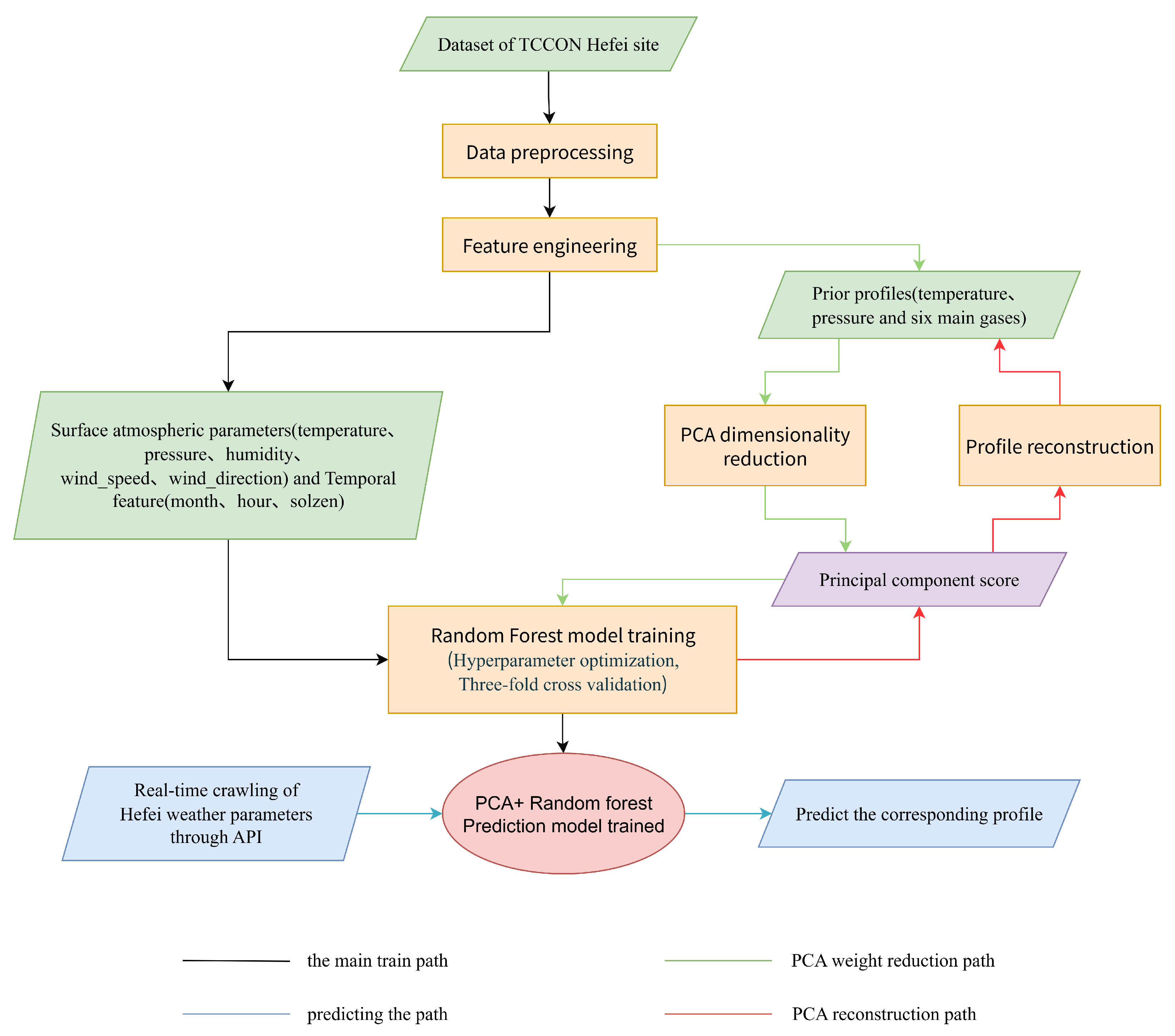
The proposed prior profile generation model offers an efficient and accurate means of producing atmospheric profiles necessary for retrieval processes. By leveraging real-time meteorological parameters as inputs, the trained model outputs profiles including temperature, pressure, and six primary atmospheric gases (Figure 1). The dataset used for model development was derived from published FTIR observations and synchronized prior profiles obtained at the TCCON station in Hefei. The TCCON network is globally recognized as the gold standard for ground-based column measurements of greenhouse gases, providing a high-quality, rigorously validated, and consistent dataset that is ideal for training robust machine learning models [22,23].

Prior to model training, the dataset underwent several quality control procedures. To address gaps in the data record, the median filling method was employed for imputation. This is a robust missing values handling method suitable for the case of skewed distributions and outliers that may exist in atmospheric science data. After filling, the profiles were also screened for physical rationality, which ensured the quality of the data and provided a reliable data basis for subsequent principal component analysis and random forest modeling.

Principal component analysis (PCA) and random forest training were implemented in the model. PCA, a classical multivariate statistical method for dimensionality reduction, transforms high-dimensional, strongly correlated vertical profile data into orthogonal, uncorrelated principal components [24]. To determine the optimal number of principal components, the cumulative variance ratiothreshold method was applied. This is mathematically expressed as:

$$R_{\mathrm{cvr}}={\displaystyle \frac{{\sum }_{i=1}^k{\lambda }_i}{{\sum }_{i=1}^M{\lambda }_i}}$$

(1)

where $R_{\mathrm{cvr}}$ represents the cumulative variance ratio, ${\lambda }_i$ denotes the eigenvalues corresponding to each principal component, k indicates the number of selected components, and M is the total number of components.

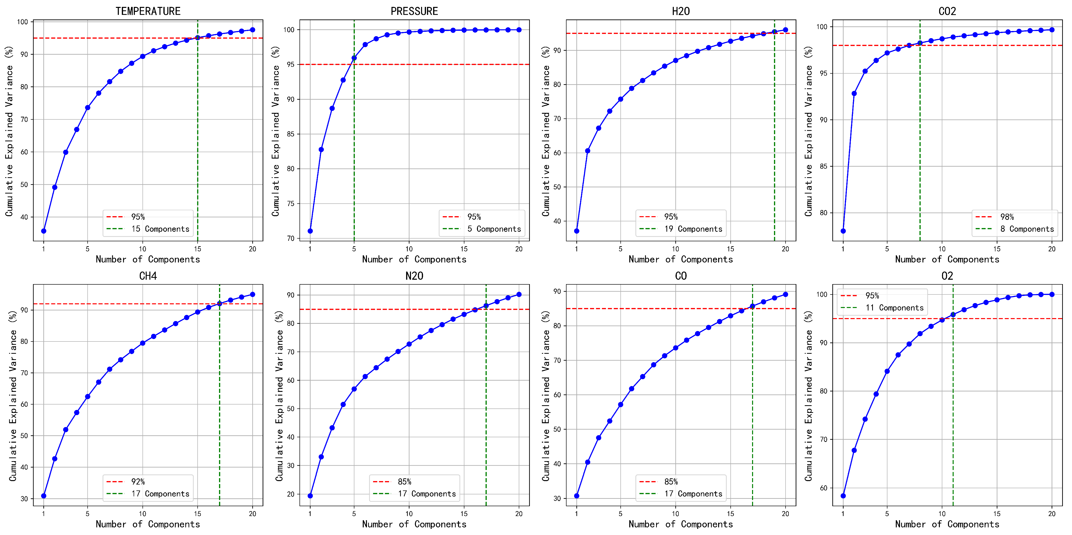
For each atmospheric profile, the minimum number of principal components necessary to achieve the preset cumulative explained variance ratio threshold was determined (Figure 2). The figure illustrates the relationship between the cumulative explained variance and the number of principal components for each profile. A red horizontal line denotes the preset variance threshold, while a green vertical line indicates the number of components required to meet this threshold. The blue curve represents the cumulative explained variance, demonstrating how additional components incrementally capture the total variance. This visualization facilitates the identification of the optimal number of principal components, balancing dimensionality reduction with information retention. Subsequently, PCA was applied to the preprocessed atmospheric profiles to reduce their dimensionality, yielding low-dimensional, uncorrelated inputs for subsequent random forest modeling.

The Random Forest algorithm was specifically chosen for its robustness to overfitting [25], its ability to handle non-linear relationships effectively, and its relatively straightforward interpretability compared to more ‘black-box’ models like deep neural networks. During training, the algorithm generates an ensemble of regression trees with diverse structures through random sampling of instances and features [26]. For a new input sample, predictions from all trees are averaged to compute the final output, as shown below:

$$\widehat{y}={\displaystyle \frac{1}{B}}\sum _{b=1}^B{f}_b\left(x\right)$$

(2)

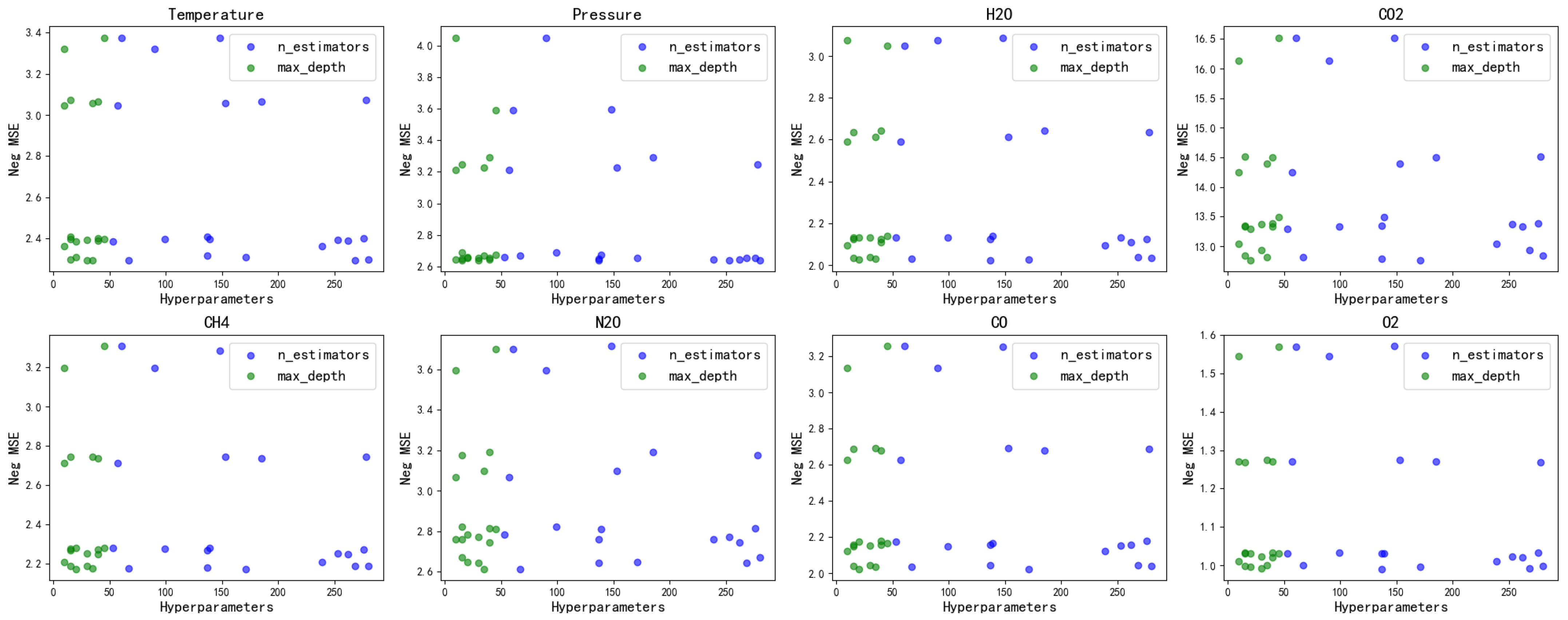
Here, $\widehat{y}$ denotes the predicted value, B represents the total number of regression trees, and $f_b\left(x\right)$ corresponds to the prediction of the b-th tree for input feature x. To enhance robustness and mitigate overfitting, cross-validation and hyperparameter tuning were performed (Figure 3). Randomized-Search-CV was utilized to explore the parameter space systematically after defining hyperparameter distributions. Notable variations in mean squared error (MSE) were observed across different hyperparameter configurations, influencing the training performance of the random forest model. As depicted in Figure 3, the MSE distributions for various atmospheric profiles exhibit differences depending on the selected hyperparameters. To mitigate this issue, we performed individualized hyperparameter optimization for each profile to determine the most effective parameter settings. The optimal hyperparameter combinations are comprehensively outlined in Appendix A.

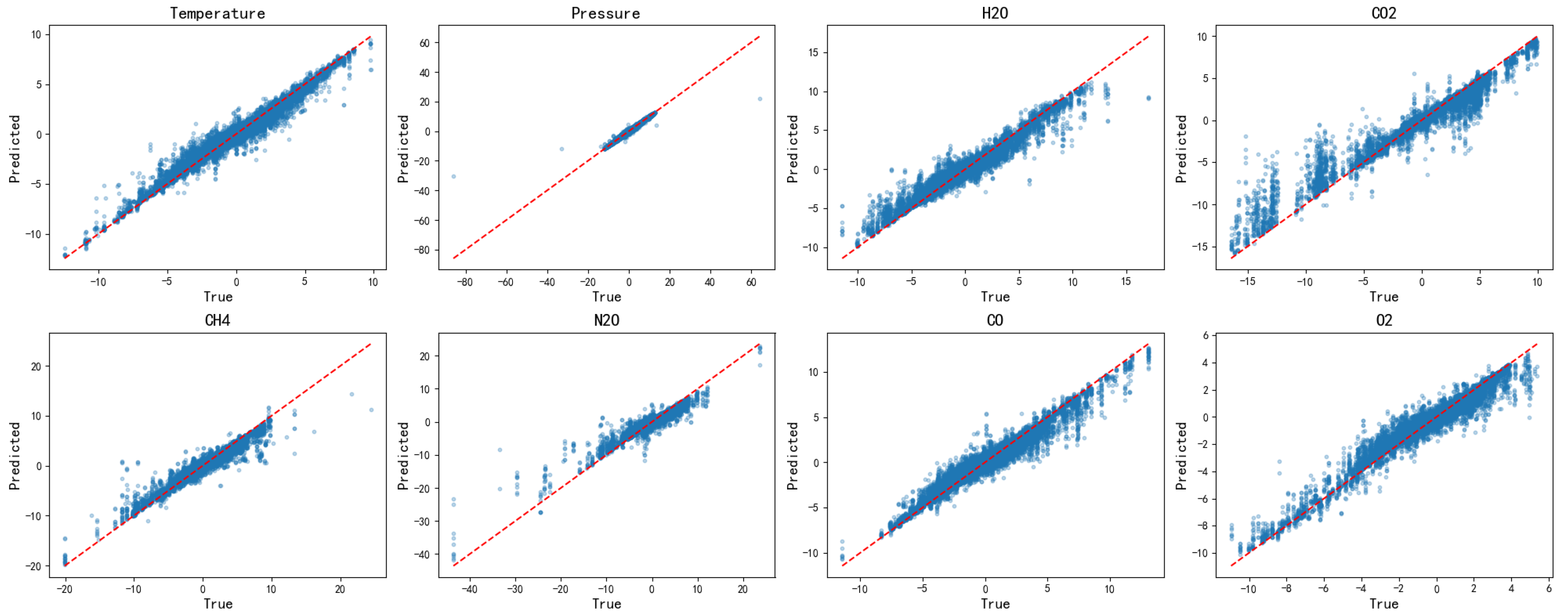
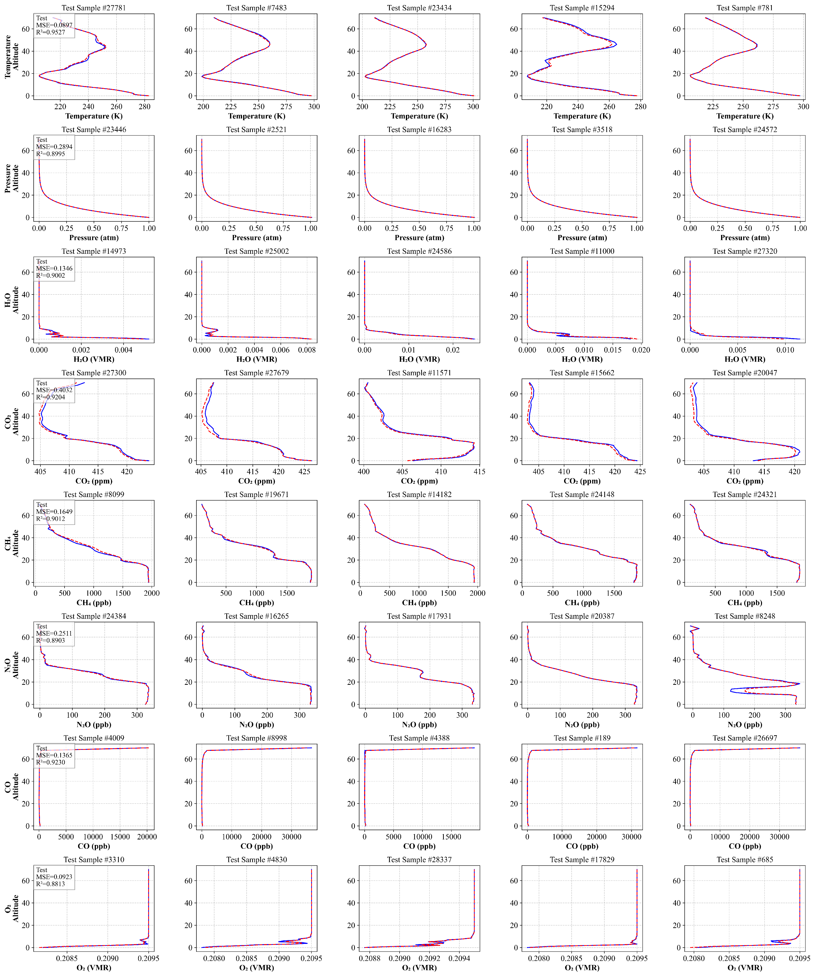
As illustrated in Figure 4, key observations include the following: Temperature, pressure, H₂O, and CO₂ exhibit tight clustering around the diagonal line, suggesting excellent model performance for these variables. In contrast, CH₄ and N₂O demonstrate slightly wider dispersion, indicative of moderate prediction uncertainty. Meanwhile, O₂ and CO show consistent patterns with minimal outliers, confirming their reliable predictions.These overall distribution characteristics validates that the random forest model effectively captures the complex nonlinear relationships between input features and principal components. This capability facilitates accurate reconstruction of atmospheric state variables from spectral data, underscoring the model’s robustness and precision.

The performance metrics in

Table 1. Performance metrics (MSE and $R^2$) of the predictive model on training and test sets.

Profile	Training Set		Test Set
	MSE	${\mathit{R}}^{\mathbf{2}}$	MSE	${\mathit{R}}^{\mathbf{2}}$
Temperature	0.0582	0.97	0.0897	0.95
Pressure	0.3141	0.90	0.2894	0.90
H2O	0.0940	0.93	0.1346	0.90
CO2	0.2878	0.94	0.4032	0.92
$C{H}_4$	0.1111	0.94	0.1649	0.90
N2O	0.1742	0.92	0.2511	0.89
CO	0.1054	0.94	0.1365	0.92
O2	0.0658	0.91	0.0923	0.88

demonstrate that the model achieves accurate fitting while maintaining strong generalization across both training and test sets. In the context of atmospheric profile modeling, the low Mean Squared Error (MSE) values indicate that the average prediction error is small relative to the natural variability of the profiles, ensuring the generated a priori information is a reliable starting point for the inversion. Concurrently, the high coefficient of determination ($R^2$) values, ranging from 0.88 to 0.97, are particularly significant [27]. An $R^2$ value exceeding 0.9 is widely considered to indicate a model that effectively explains the variance of the reference data. Notably, the model demonstrates strong generalization for our primary target, CO₂, achieving an $R^2$ of 0.94 on the training set and maintaining a high value of 0.92 on the test set. This confirms that the model has successfully learned the key variability characteristics of the gas profiles without significant overfitting, a prerequisite for enhancing retrieval accuracy [28]. Detailed evaluation of the model’s performance on the test set is provided in Appendix C. The integration of real-time meteorological parameters via the API (api.openweathermap.org) [29] enables the generation of corresponding atmospheric profiles at specific times.

Due to the limited size of the training dataset, geographic coordinates such as longitude and latitude were not utilized as features. Consequently, the model’s current applicability is confined to the Hefei region. Future work is expected to incorporate datasets from diverse geographical locations to expand the model’s regional applicability.

3. Data Processing

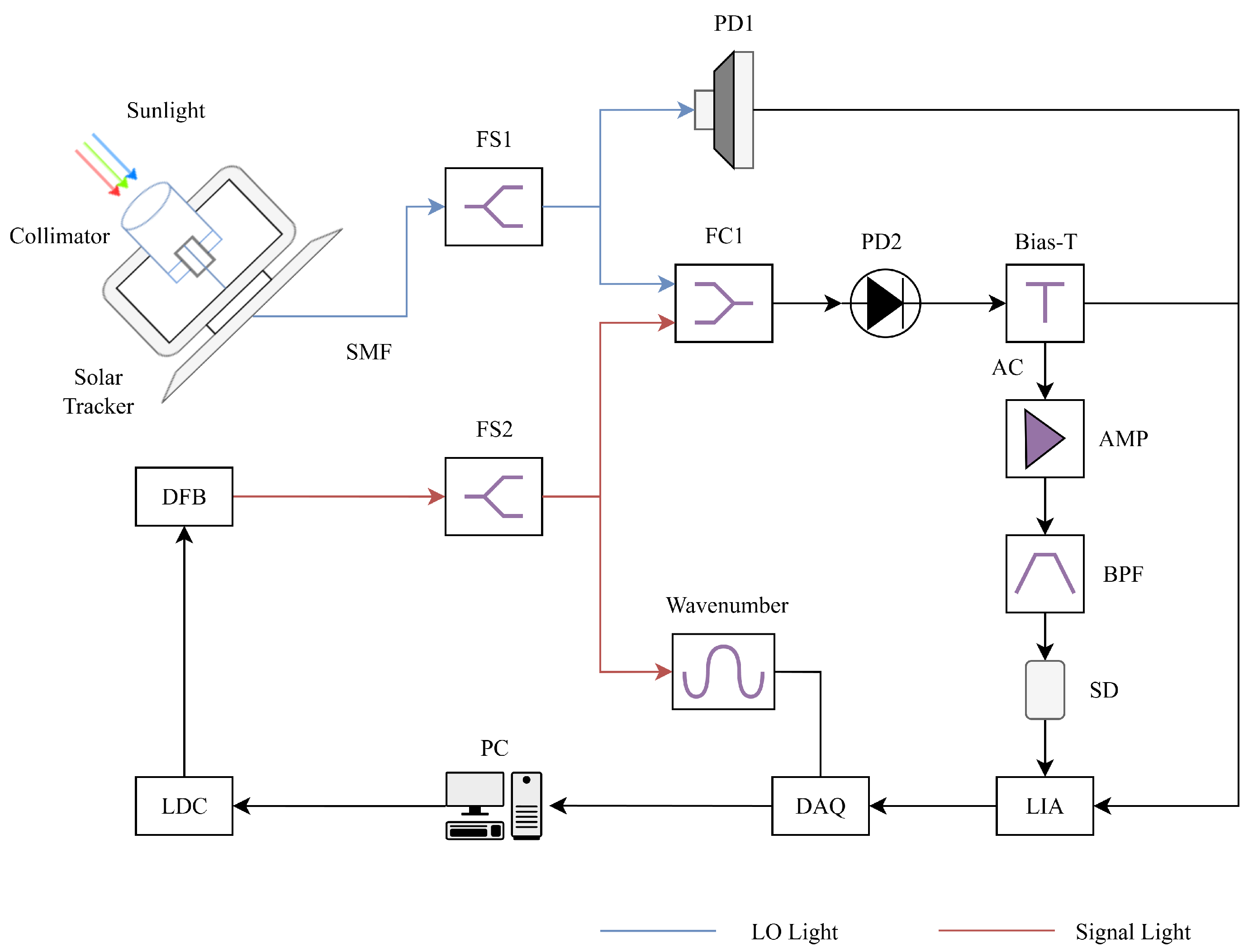
With the prior profile generation model established, we now focus on preprocessing the raw LHR signals to ensure high-quality data for subsequent retrieval analysis. The raw signals were acquired at a spectral resolution of $0.012{\mathrm{cm}}^{-1}$ in Hefei, China ($31.9^{\circ }\mathrm{N},117.{16}^{\circ }\mathrm{E}$), on 22 August 2025, through point-by-point scanning. The experimental setup and signal acquisition process are illustrated in Figure 5. 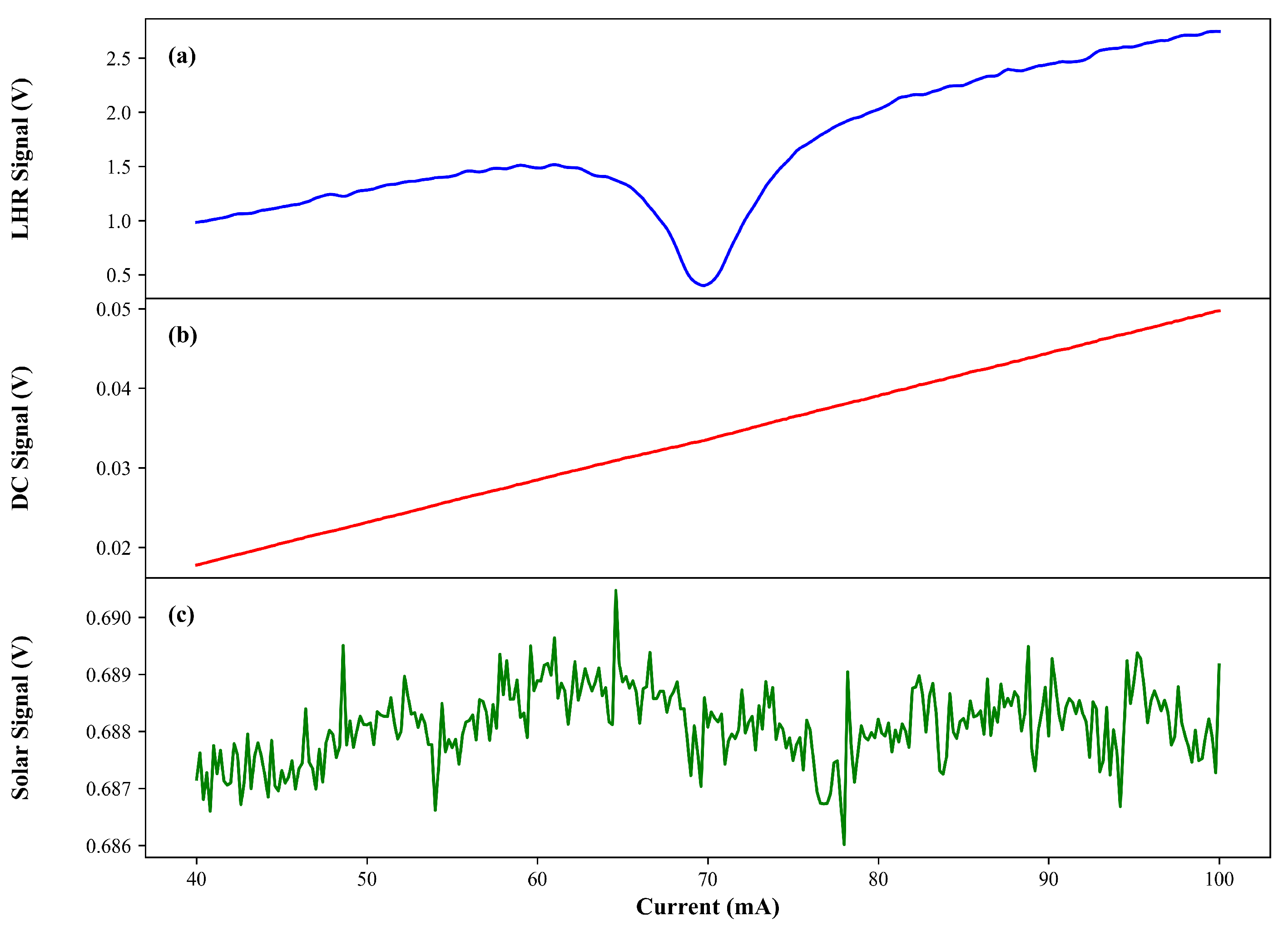While the experimental details are beyond the scope of this article, further information can be found in the following references [30,31,32,33]. Before proceeding with data retrieval, the raw signals (Figure 6) underwent several preprocessing steps, including solar signal correction, normalization, and wavenumber offset calibration.

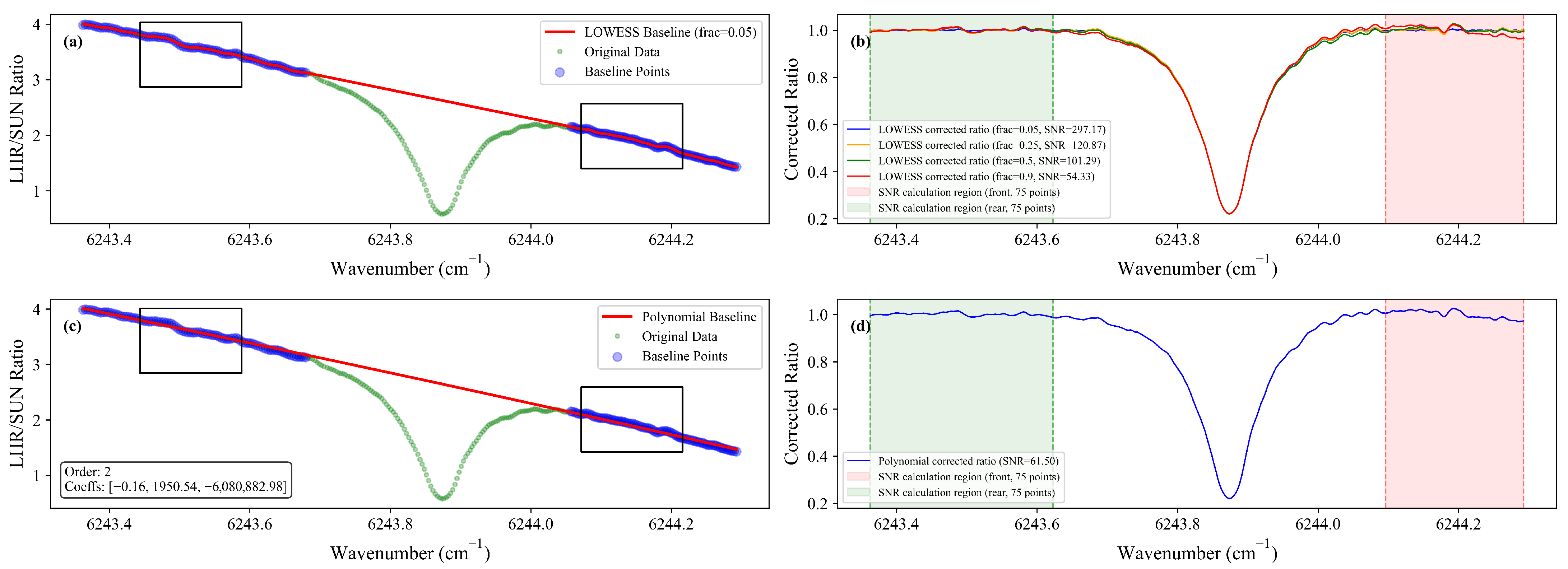
To mitigate fluctuations in the solar signal [34], the LHR signal was normalized by dividing it with the synchronously acquired solar signal, effectively eliminating variations caused by solar instability. Subsequently, the Locally Weighted Scatterplot Smoothing (LOWESS) adaptive baseline fitting method was applied to further refine the normalized signal, addressing both baseline drift and noise interference (Figure 7).

The LOWESS method estimates a slowly varying baseline by performing weighted least squares regression within the local neighborhood of each wavenumber point. This involves minimizing the following objective function:

$$\begin{array}{c}\hfill \beta \left({\nu }_i\right)=arg\underset{\beta }{min}\sum _{j}K\left({\displaystyle \frac{|{\nu }_j-{\nu }_i|}{h}}\right)\times {\left[R\left({\nu }_j\right)-({\beta }_0+{\beta }_1{\nu }_j)\right]}^2\end{array}$$

(3)

Here, $\beta ={[{\beta }_0,{\beta }_1]}^T$ denotes the regression coefficients at wavenumber ${\nu }_i$, h is the bandwidth controlling the local neighborhood size, and $K\left(u\right)$ is the kernel function weighting neighboring points based on their distance from ${\nu }_i$. The kernel function is defined as:

$$K\left(u\right)={(1-|u|}^3{)}^3\times {\mathbf{1}}_{\left|u\right|<1}$$

(4)

The indicator function ${\mathbf{1}}_{\left|u\right|<1}$ equals 1 when $\left|u\right|<1$ and 0 otherwise, defining weight decay for neighboring points. Non-absorbing spectral regions are used to construct the dataset, ensuring only relevant data contribute to baseline estimation.

The smoothing parameter h, which determines the bandwidth for local regression in LOWESS, is directly proportional to the total number of data points N, scaled by the fraction specified via the frac parameter. Mathematically, this relationship can be expressed as $h=\mathit{frac}\times N$, where frac controls the proportion of data points included in each local neighborhood. A smaller frac value results in a narrower bandwidth, capturing finer details but potentially increasing noise sensitivity, while a larger frac smooths over broader regions, mitigating noise but risking the loss of subtle spectral features. After determining the appropriate smoothing parameter, linear interpolation is applied across the entire spectral domain, followed by normalization using the following equation:

$$R_{\mathrm{corr}}\left(\nu \right)={\displaystyle \frac{R\left(\nu \right)}{b\left(\nu \right)}}$$

(5)

Here, $R_{\mathrm{corr}}\left(\nu \right)$ is the spectral signal after baseline correction, where $R\left(\nu \right)$ is the originally measured spectral signal and $b\left(\nu \right)$ denotes the estimated baseline derived via the LOWESS procedure. To assess the performance of various baseline fitting methods, 75 data points from before and after the LHR measurement at 9:52:11 were chosen for signal-to-noise ratio (SNR) calculations. As illustrated in Figure 7b,d, the LOWESS method achieves an SNR value of 297.17 when frac = 0.05, which is approximately four times higher than the SNR of 61.5 obtained using polynomial fitting.

This substantial improvement in SNR directly contributes to enhanced retrieval accuracy, as reduced noise levels facilitate clearer differentiation of weak absorption features from background fluctuations. Additionally, the frac parameter in LOWESS offers precise control over the degree of smoothing, as illustrated in Figure 7b. This tunable balance between noise suppression and the retention of subtle spectral characteristics underscores the adaptability of LOWESS, particularly in complex spectral regions, ultimately leading to improved sensitivity and reliability in spectral inversion processes.

To address residual micro-drift inherent in point-by-point scanning and wavelength meter calibration, a correlation coefficient-based calibration method was employed. Specifically, the measured spectrum is shifted relative to a forward reference spectrum, and the correlation coefficient is computed at each offset. Through an iterative refinement process involving interpolation, the wavelength offset corresponding to the maximum correlation coefficient is accurately determined, ensuring high-precision wavelength correction. This step is critical because even minor spectral shifts, on the order of a fraction of the instrument’s resolution, can introduce significant systematic errors in the retrieved column abundance by causing a mismatch between the measured spectrum and the forward model. With these preprocessing steps completed, the data were prepared for subsequent retrieval.

4. Data Retrieval

After completing the data preprocessing, atmospheric parameters were retrieved using the Optimal Estimation Method (OEM), as originally described by Rodgers (1977) [35] and further refined in recent studies (e.g., [36,37]). The OEM framework establishes a mathematical relationship between the measurements and the atmospheric state vector x, expressed as:

$$\begin{array}{c}\hfill y_m=F(x,a,b,c)+ϵ,\end{array}$$

(6)

Here, $y_m$ denotes the measurement vector of the observed radiance spectrum. The forward model $F\left(x\right)$ simulates the measured spectrum based on the atmospheric state vector x, while $ϵ$ represents the combined effects of measurement noise and model uncertainties.

To address non-selective absorption and residual baseline effects within the spectral region, a second-order polynomial baseline correction was integrated into the retrieval process, consistent with established methodologies for spectroscopic data analysis [13]. Parameters a, b, and c represent the coefficients of the quadratic polynomial baseline. The retrieval procedure employs an iterative optimization scheme based on Bayesian inference, utilizing Gaussian probability density functions to minimize the cost function [38,39]. This approach has been widely adopted in atmospheric remote sensing applications.

The atmospheric transmission spectrum is modeled using the radiative transfer forward model F, incorporating spectroscopic databases such as HITRAN or GEISA. This model is implemented within Py4CAtS (Python for Computational Atmospheric Spectroscopy, version 4.0.0), a Python-based radiative transfer package. Py4CAtS re-implements the Fortran-encoded GARLIC framework, which is primarily designed for infrared and microwave radiative transfer calculations. To ensure high accuracy, Py4CAtS employs a line-by-line integration approach. This method determines atmospheric transmittance by computing individual spectral lines, thereby providing precise results.

Py4CAtS operates by solving the radiative transfer equation (Equation (7)) for each spectral line individually, enabling high precision in modeling the interaction between radiation and atmospheric constituents. The core principle involves calculating both absorption and emission contributions of individual molecular transitions along a defined atmospheric path. This process leverages detailed spectroscopic databases such as HITRAN or GEISA to retrieve accurate line parameters, including line positions, intensities, and broadening coefficients. This method has also been successfully applied in atmospheric inversion studies, for example by Wang et al. (2023) [13].

The radiative transfer equation is expressed as:

$$\begin{array}{c}\hfill I_{\nu }\left(s\right)=I_{\nu }\left(0\right)e^{-{\tau }_{\nu }\left(s\right)}+{\int }_0^s{S}_{\nu }\left(s^{\prime }\right)e^{-{\tau }_{\nu }(s^{\prime },s)}{\kappa }_{\nu }\left(s^{\prime }\right)d{s}^{\prime },\end{array}$$

(7)

where $I_{\nu }\left(s\right)$ is the specific intensity at optical depth s, $I_{\nu }\left(0\right)$ the initial intensity, ${\tau }_{\nu }\left(s\right)$ the total optical depth up to s, $S_{\nu }\left(s^{\prime }\right)$ the source function, and ${\kappa }_{\nu }\left(s^{\prime }\right)$ the absorption coefficient at $s^{\prime }$.

The relationship between total optical depth (${\tau }_{\nu }$) and atmospheric transmittance ($T_v$) is established using the Beer-Lambert law. Transmittance is defined as the fraction of incident radiation that passes through a medium, which can be mathematically expressed as:

$$T_{\nu }=e^{-{\tau }_{\nu }}$$

(8)

Here, $T_{\nu }$ denotes the transmittance at a specific wavenumber $\nu$, while ${\tau }_{\nu }$ represents the corresponding total optical depth.

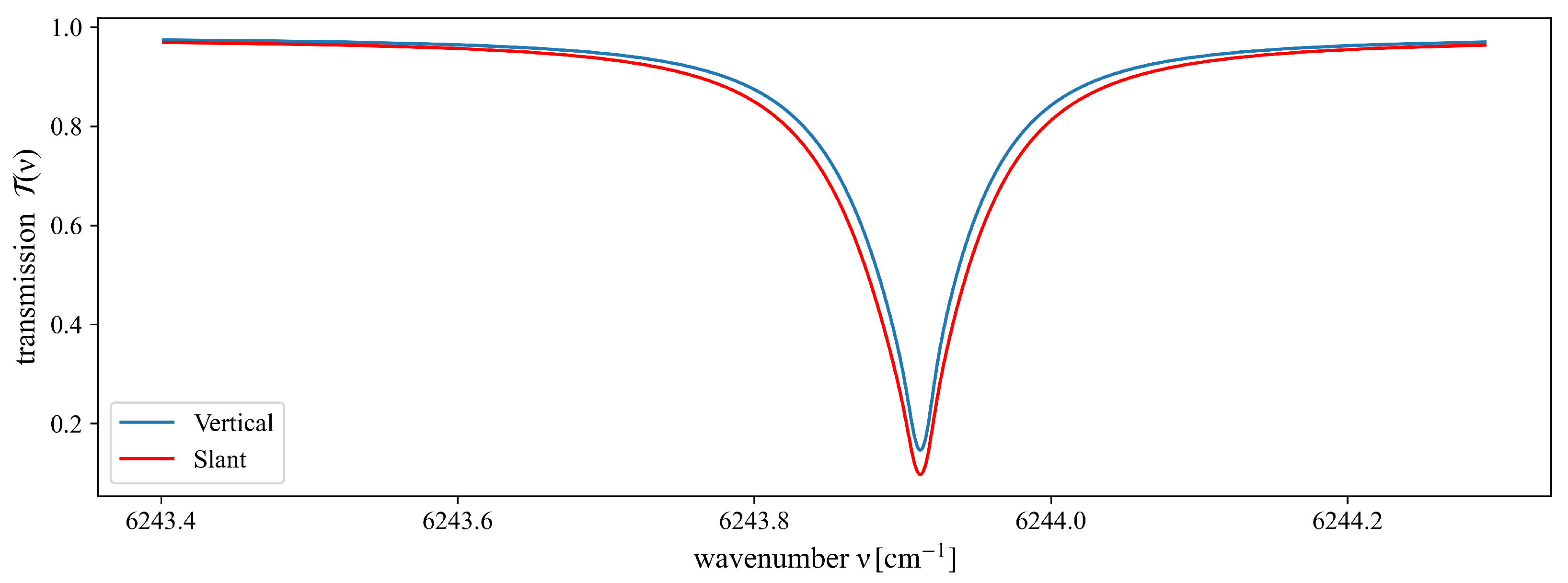
The transformation from vertical to slant-path transmittance is essential for accurately modeling atmospheric absorption along the observation path. This process involves modifying the optical depth based on the solar zenith angle ($\theta$). By applying the Beer-Lambert law, the relationship between vertical ($T_v$) and slant-path ($T_s$) transmittance can be formulated as follows:

$$T_s=T_v^{\frac{1}{cos\left(\theta \right)}}$$

(9)

The air mass factor (AMF), defined as $\mathrm{AMF}=\frac{1}{cos\left(\theta \right)}$, quantifies the elongation of the optical path due to the increased path length at non-zero zenith angles. For absorbing media, where $T_v<1$, it follows that $T_s<T_v$ when $\mathrm{AMF}>1$. This result aligns with the physical intuition that longer optical paths lead to greater absorption.

By integrating over all contributing spectral lines, Py4CAtS constructs a comprehensive representation of the atmospheric transmission spectrum, thereby ensuring consistency with physical principles and observed data.

Furthermore, the incorporation of instrumental effects, particularly the ILS, significantly improves the accuracy of the simulated spectra, aligning them more closely with real-world measurement characteristics. The calculation of the slant-path transmittance spectrum is performed prior to the application of instrument line shape (ILS) convolution. Specifically, zenith angle correction is applied to the radiative transfer modeling, ensuring a more precise depiction of atmospheric absorption along the designated observation path (Figure 8).

The forward calculation program computes the forward spectrum and Jacobian matrix. The input parameters include atmospheric profiles (pressure, temperature, and atmospheric species), the Instrument Line Shape (ILS) (Figure 9), and the solar zenith angle.

In the inverse program, the forward calculation is iteratively performed. This iterative process minimizes the cost function using the Levenberg-Marquardt (LM) algorithm. The LM algorithm was selected as it provides a robust and efficient compromise between the Gauss–Newton algorithm and the method of gradient descent, making it well-suited for non-linear least-squares problems common in atmospheric retrieval. The state vectors in this study represent the retrieved atmospheric parameters.

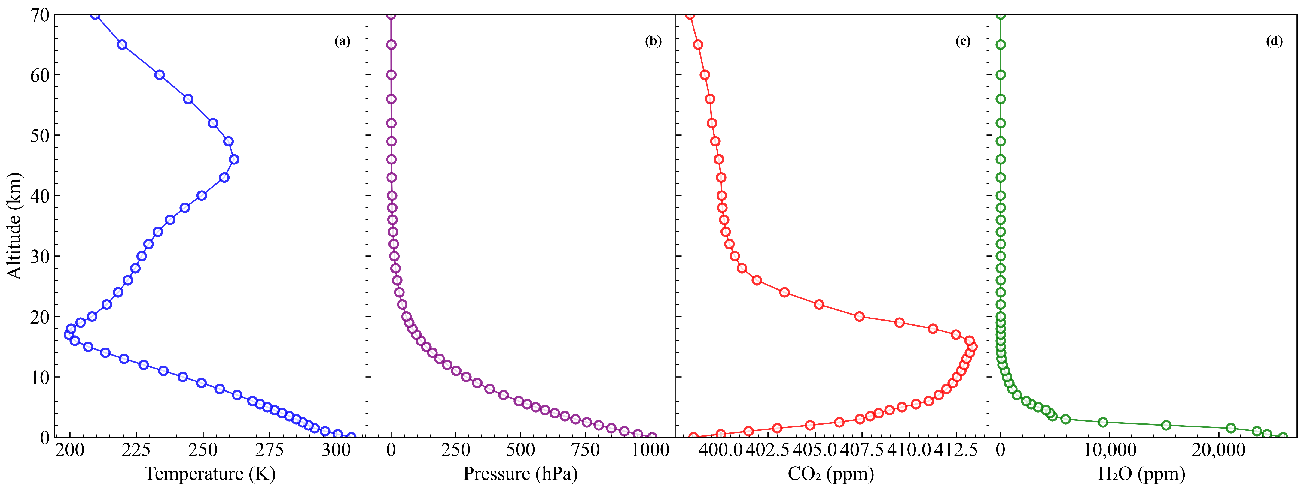
To illustrate the data retrieval process, representative data collected at 9:52:11 on 22 August 2025 were selected. The pressure and temperature profiles used for data retrieval are shown in Figure 10, both derived from the trained model. The atmosphere was discretized into 45 layers from the surface to 70 km, with varying altitude resolutions of 0.5, 1, 2, 3, 4, and 4 km, respectively. The prior profiles of CO₂ and H₂O were also obtained from the model output. The real-time weather parameters used as input to the model are detailed in Appendix B. Additionally, the real-time solar zenith angles were determined using Pysolar [40], consistent with the NOAA solar calculator [41].

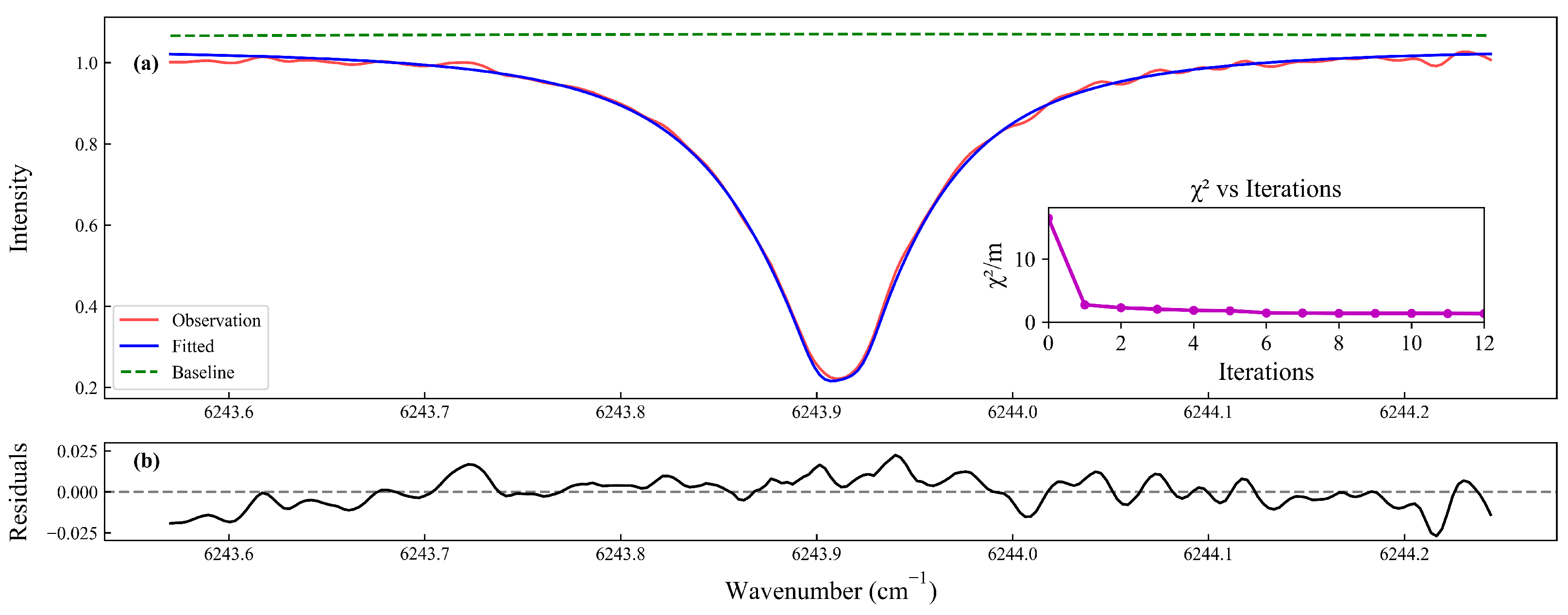
The LM iteration process converges when $\Delta {\chi }^2/{\chi }^2$ falls below $1\times {10}^{-3}$, with a maximum limit of 20 iterations. For effective retrieval, the ultimate cost function (${\chi }^2$) should approximate the size of the measurement vector (m). The inversion results are shown in Figure 11. In addition to the scaling factor, the three parameters of the quadratic polynomial baseline (Figure 12) were iteratively adjusted to eliminate unselected power contributions. The fitting spectrum, baseline, and residuals align with the point intervals of the preprocessed LHR data.

The iterative processes are depicted in the inset of Figure 11a, where ${\chi }^2/m$ approaches unity after 10 iterations. As illustrated in Figure 12b, even when a trial step causes the parameter b to exceed its expected range during early iterations, the algorithm effectively corrects the deviation through subsequent iterations, demonstrating robust convergence behavior. After convergence, the retrieved CO₂ profiles were calculated by multiplying the retrieved scaling factor with the relative a priori profile. Using the water vapor profile from the model, the dry-air mixing ratio ($X_{C{O}_2}$) was calculated as approximately 421.77 ppm.

As illustrated in Figure 13, consecutive measurements conducted on 22 August 2025, demonstrate the high precision of the $X_{C{O}_2}$ retrieval process. The retrieved $X_{C{O}_2}$ values exhibit a statistical mean of 422.04 ppm with a standard deviation of approximately 0.68 ppm.

5. Discussion

This study presents a novel framework for retrieving atmospheric parameters by integrating laser heterodyne radiometry (LHR) with random forest-based prior profile generation. The LHR experiment was conducted in Hefei, China, on 22 August 2025. Real-time weather parameters were employed to generate prior profiles using the developed prediction model, while LOWESS was applied to preprocess the LHR signals, leading to a robust set of $X_{C{O}_2}$ inversion results. The precision of our retrievals was evaluated by calculating the relative uncertainty of the $X_{C{O}_2}$ time series, defined as the standard deviation divided by the mean:

$$u\left(X_{C{O}_2}\right)=\left({\displaystyle \frac{{\mathrm{std}}_{X_{C{O}_2}}}{{\mathrm{mean}}_{X_{C{O}_2}}}}\right)\times 100$$

(10)

where ${\mathrm{std}}_{X_{C{O}_2}}$ is the standard deviation and ${\mathrm{mean}}_{X_{C{O}_2}}$ is the statistical mean of the retrieved $X_{C{O}_2}$ values over the measurement period. Based on a standard deviation of 0.68 ppm and a mean of 422.04 ppm, this calculation yielded a relative uncertainty of just 0.16%. This high level of precision is particularly notable, as it is even lower than the 0.17–0.5% relative uncertainty range previously reported for similar state-of-the-art LHR systems by Wang et al. (2020) [42]. This represents a notable improvement in retrieval precision over conventional methods that rely on static climatological profiles, which can introduce additional variance and bias. We attribute this enhanced precision to two key innovations introduced in this work. First, the use of dynamic, real-time a priori profiles generated by our random forest model provides a more accurate initial state for the inversion, reducing biases that can arise from using static, climatological profiles. Second, our application of the LOWESS method for baseline correction resulted in a nearly five-fold improvement in the signal-to-noise ratio of the preprocessed spectra. A cleaner input spectrum with less residual noise directly translates to a more stable and precise inversion, as predicted by optimal estimation theory. The stability of our results is further demonstrated by the fact that the retrieved $X_{C{O}_2}$ values remained tightly clustered around the mean, with only minor fluctuations, despite variations in the solar zenith angle (and thus the air mass) during the two-hour measurement period. This robustness confirms that our integrated methodology—combining a machine learning-based prior with advanced signal processing—effectively mitigates the primary sources of random error, namely system noise and retrieval instabilities.

In terms of computational efficiency, the random forest-based approach demonstrates significant advantages over traditional climatological models. By leveraging real-time meteorological inputs, the model reduces reliance on static datasets and ensures adaptability to dynamic atmospheric conditions. This contrasts with conventional methods that often require extensive precomputed libraries, leading to higher computational overhead. Moreover, the use of Py4CAtS for radiative transfer modeling ensures compatibility with high-resolution spectroscopic databases like HITRAN and GEISA, further enhancing retrieval precision.

The applications for this high-precision monitoring framework are not limited to atmospheric science but extend into several other disciplines. For example, in agriculture and ecosystem science, continuous, real-time monitoring of column CO₂ offers a powerful way to validate carbon flux models. Deploying LHR instruments over a cornfield or a forest would allow researchers to directly track the daily and seasonal drawdown of atmospheric CO₂, providing a top-down measure of net ecosystem exchange (NEE). This integrated signal, which captures the balance of plant photosynthesis and soil respiration, is invaluable for developing climate-smart farming techniques, improving crop yield forecasts, and verifying the success of carbon sequestration projects. This methodology could be equally transformative for urban planning and public health. A network of LHR instruments spread across a city could map the urban CO₂ dome with high precision, allowing city planners to pinpoint and quantify major emission hotspots like traffic corridors and industrial parks. Such a network would offer near real-time feedback on the effectiveness of new emission reduction policies. And because CO₂ is often co-emitted with other harmful air pollutants, these measurements could also serve as a vital proxy for tracking air quality and informing public health advisories.

Despite the advancements achieved, certain limitations remain. The model is currently region-specific, optimized for the Hefei area, and may require adaptation for use in other geographic locations with differing climatic conditions. Extreme weather or anomalous atmospheric phenomena could also impact the performance of the random forest-based prior profile generation. Future work will focus on developing adaptive models to handle diverse environmental conditions while extending the methodology to include additional greenhouse gases such as CH₄ and N₂O, thereby enhancing its applicability. Further improvements aim to refine measurement accuracy by enabling all points of the prior profile to participate in the inversion process under physical constraints, moving beyond simple scaling factor adjustments.

The implementation of the prior profile generation model, data preprocessing, and baseline-corrected inversion algorithm in Python establishes a robust foundation for operational deployment. These components can be integrated into an end-to-end real-time system for continuous atmospheric monitoring. The methodology is compatible with automated processing, making it suitable for long-term observational studies and climate change research. Future work will incorporate advanced algorithms to enable periodic inversions, offering deeper insights into seasonal and annual variations of atmospheric CO₂ and supporting global atmospheric monitoring efforts.

6. Conclusions

This study introduces a novel methodology for generating atmospheric profiles using a random forest-based model optimized for the Hefei region. Unlike traditional methods that rely on climatological or meteorological model data, our approach utilizes real-time ground-level meteorological parameters as inputs, thereby enhancing both accuracy and computational efficiency in prior profile generation. The integration of high-resolution laser heterodyne radiometer (LHR) spectroscopy, employing a distributed feedback (DFB) laser operating at $1601\mathrm{nm}$, enabled precise measurements of atmospheric CO₂ concentrations. Additionally, the correlation coefficient-based wavenumber calibration method ensured spectral accuracy, a critical factor for reliable atmospheric retrievals.

The retrieved results demonstrated a uniform error distribution with well-constrained uncertainties, validating the precision and robustness of the inversion process. Compared to conventional methods relying on static climatological profiles, our approach reduced uncertainty by approximately 0.175%. Successful inversion analysis of the continuous dataset collected on 22 August 2025, confirmed the system’s capability to handle real-world atmospheric conditions effectively.