

Evaluation of the Impact of Morphological Differences on Scale Effects in Green Tide Area Estimation


Abstract

1. Introduction
2. Materials and Methods
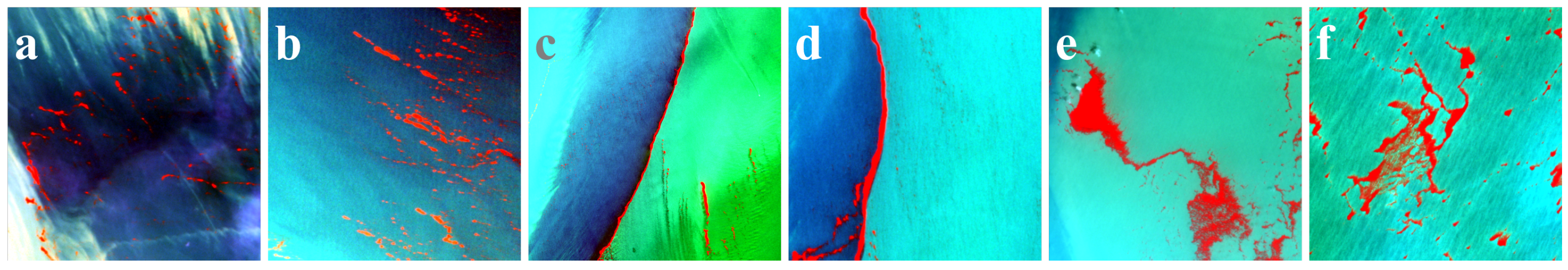
2.1. Data Collection and Green Tide Detection
2.2. Patch Segmentation
- If is a target pixel and at least one neighboring pixel is already labeled, the current pixel is labeled with the same label as the neighboring pixel.
- If multiple neighboring pixels have different labels, their equivalence relationship is recorded in the equivalence table, and the current pixel is assigned the smaller label.
- A new label is assigned to the current pixel if no neighboring pixels are labeled.
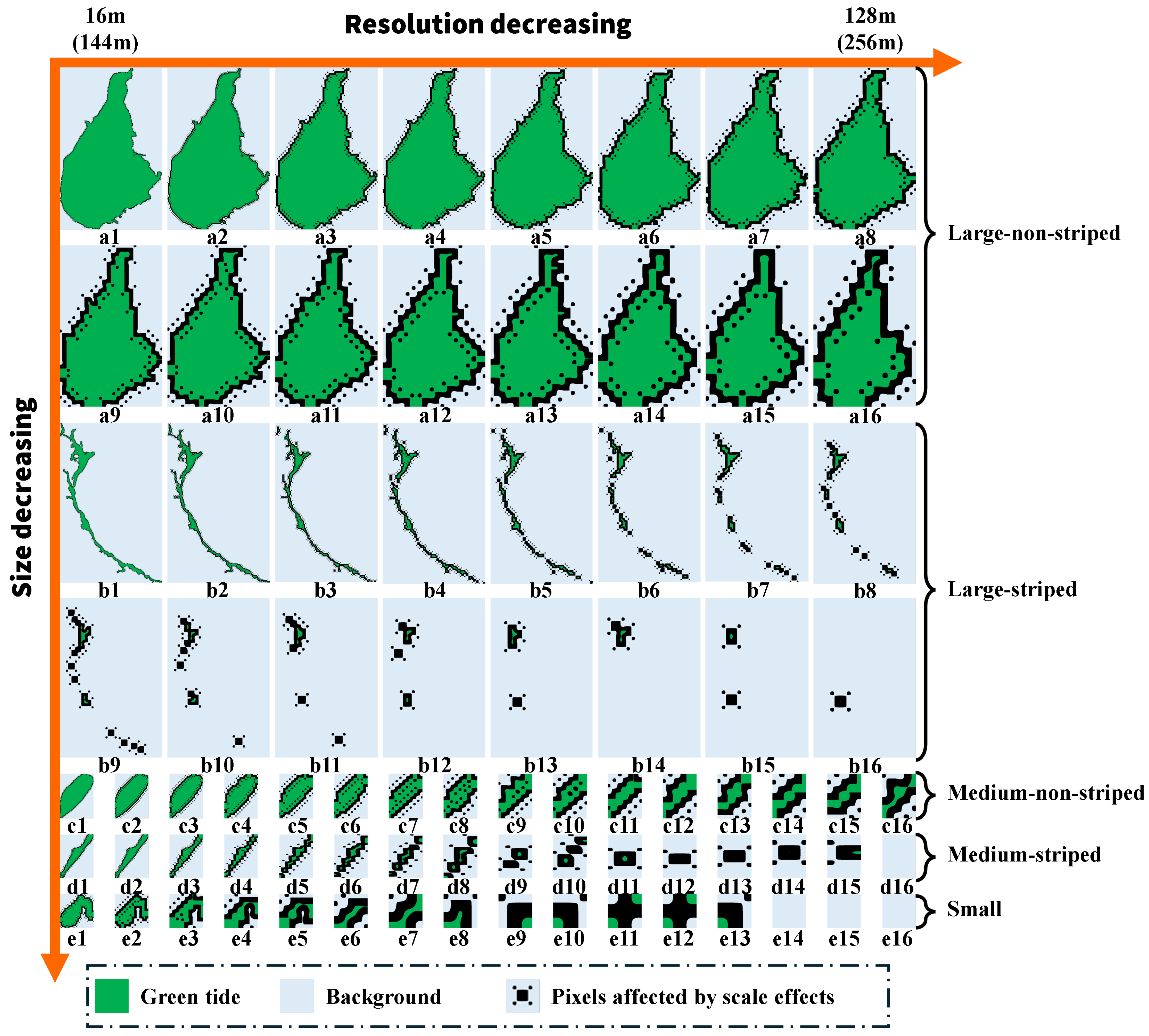
2.3. Patch Classification Based on Size
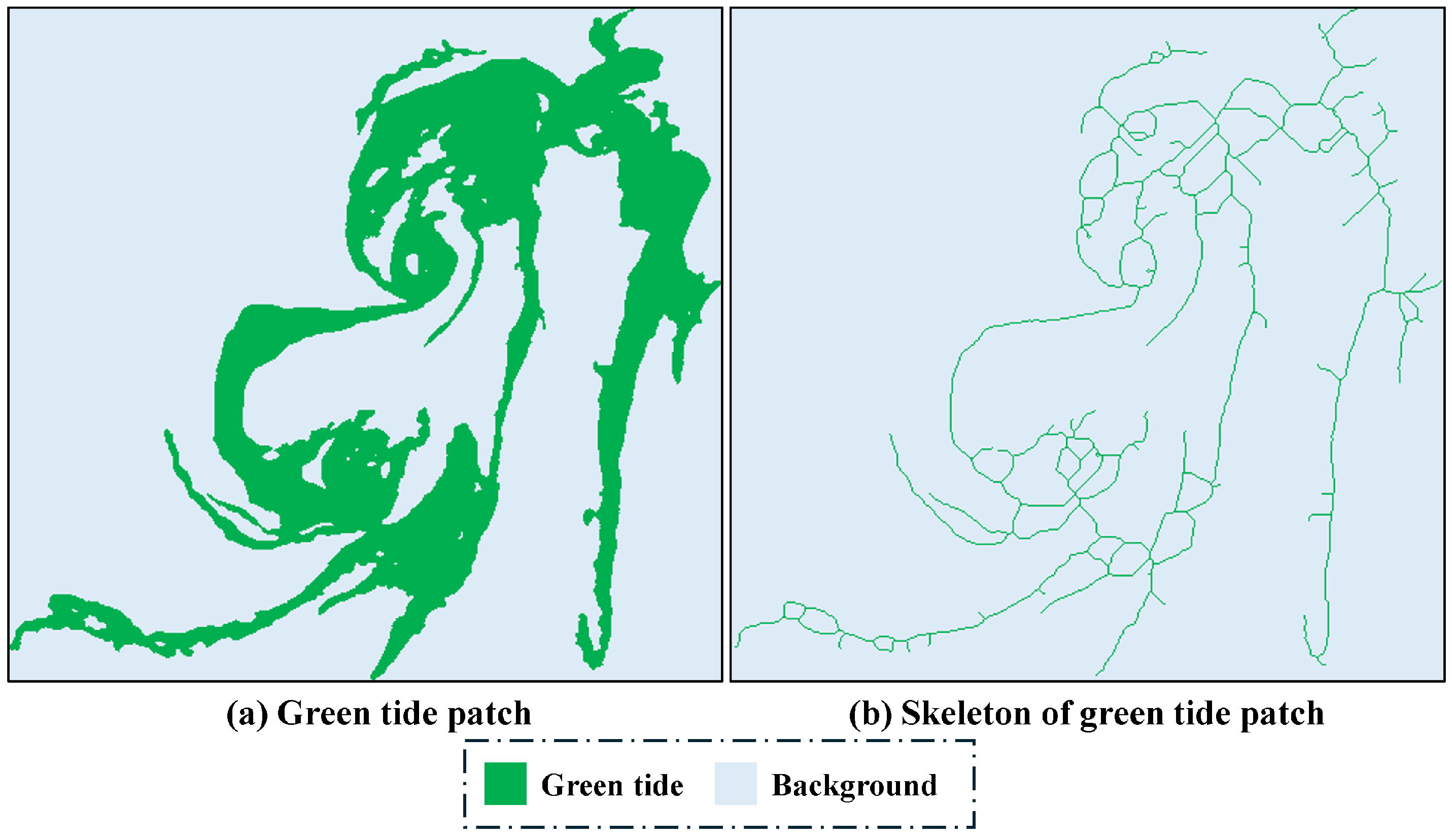
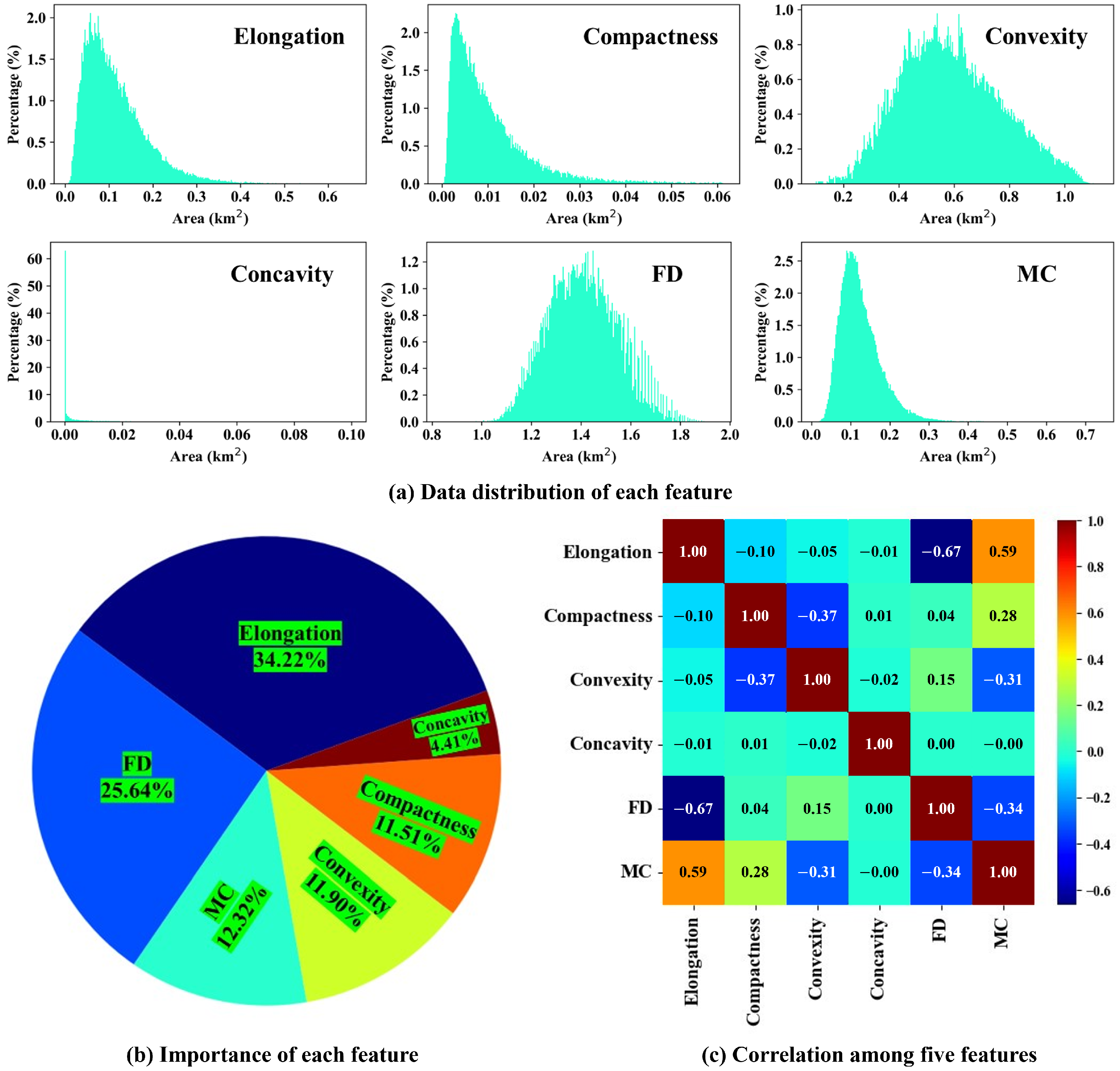
2.4. Elongation, Compactness, Convexity and Concavity
2.5. Fractal Dimension
2.5.1. Box-Counting Method
2.5.2. Orientation Calculation
2.5.3. Image Rotation
2.5.4. Image Padding
2.5.5. Calculation of Fractal Dimension
2.6. Morphological Complexity
2.7. Optimal Feature Selection
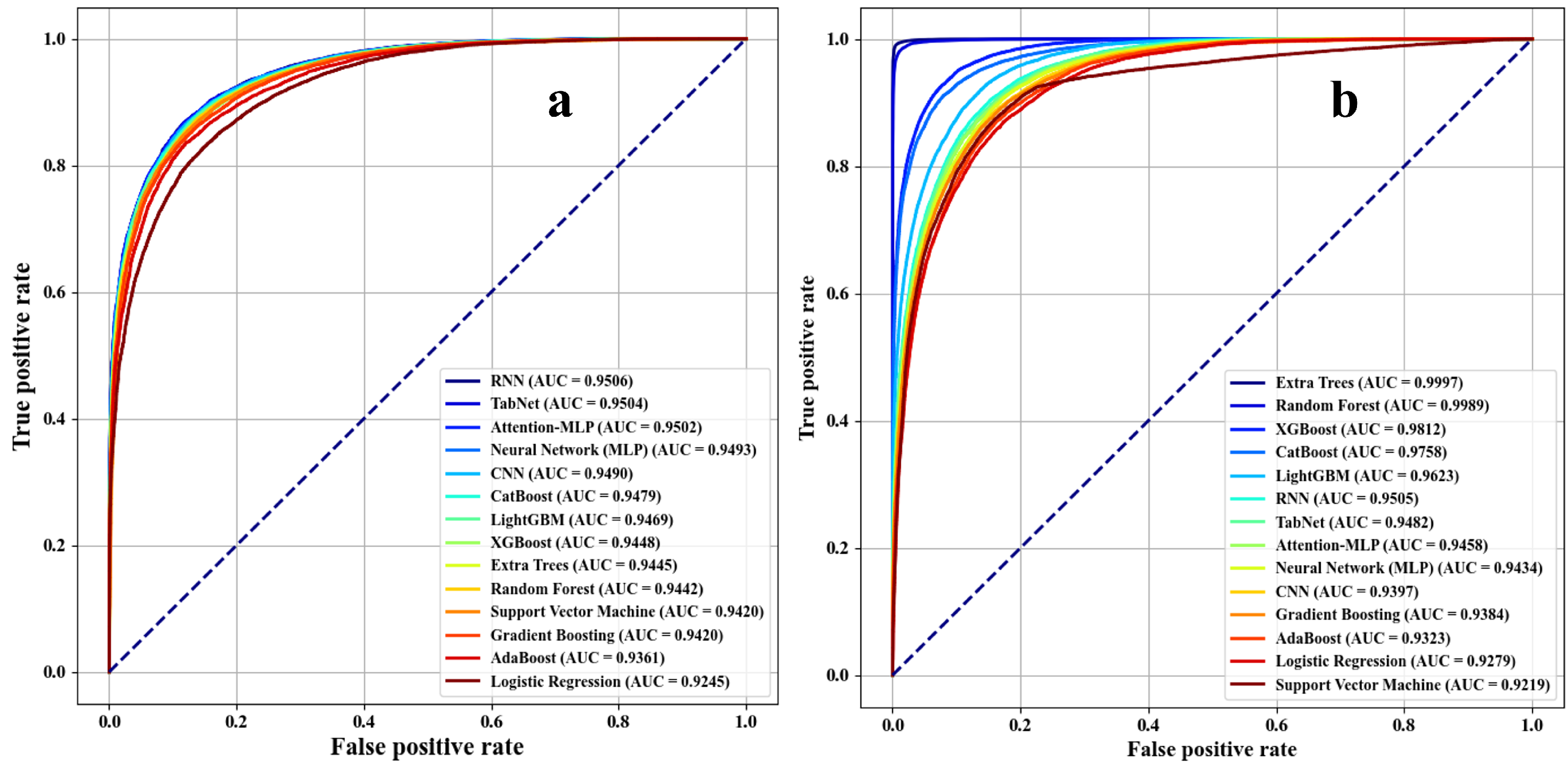
2.8. Classification Based on Morphological Features
3. Results
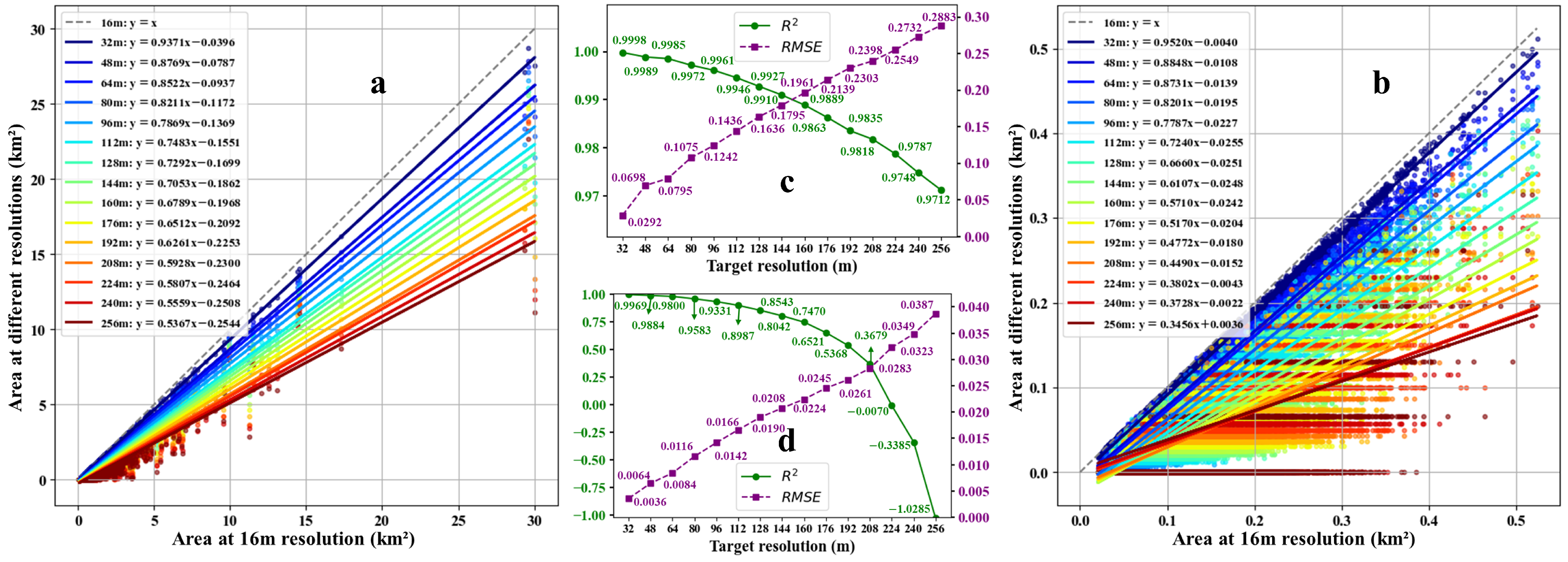
3.1. Striped Type
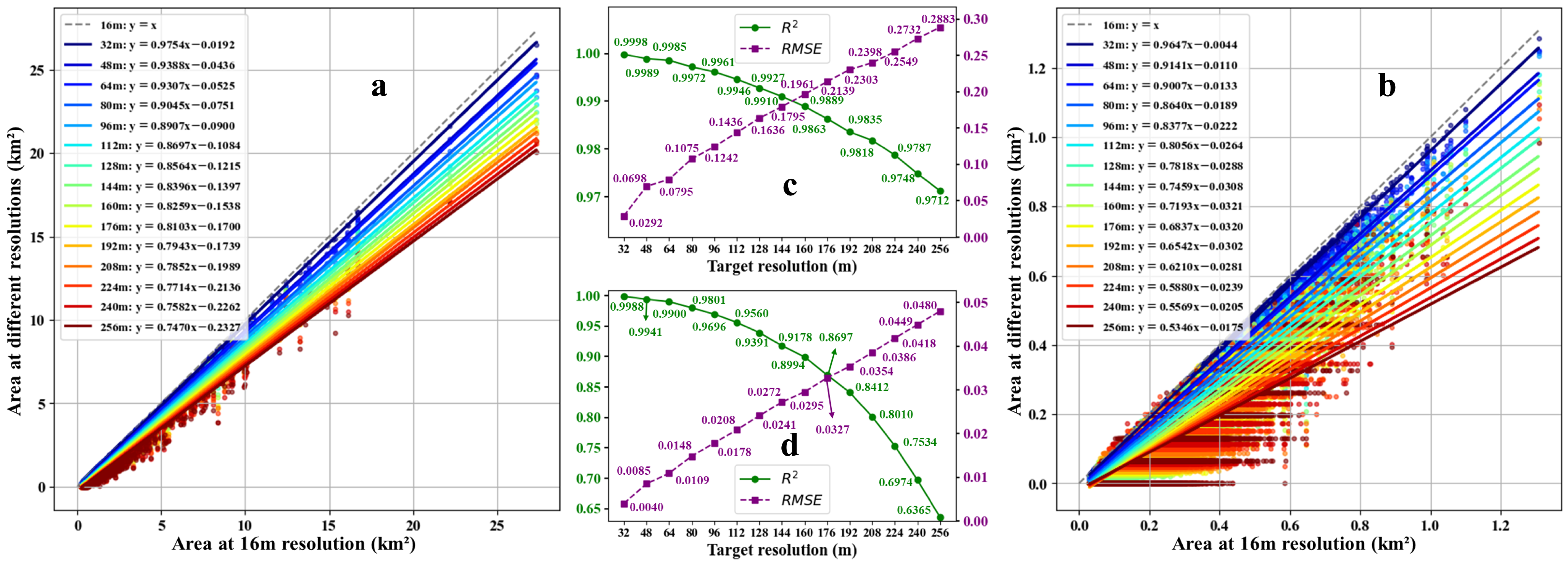
3.2. Non-Striped Type
3.3. Small Type
4. Discussion
4.1. Scale Effects and Morphological Sensitivity of Green Tide Patches
4.2. Potential of Super-Resolution Methods in Green Tide Area Estimation
5. Conclusions
Author Contributions
Funding
Data Availability Statement
Acknowledgments
Conflicts of Interest
References
- Xia, Z.; Liu, J.; Zhao, S.; Sun, Y.; Cui, Q.; Wu, L.; Gao, S.; Zhang, J.; He, P. Review of the development of the green tide and the process of control in the southern Yellow Sea in 2022. Estuar. Coast. Shelf Sci. 2024, 302, 108772. [Google Scholar] [CrossRef]
- Feng, G.; Zeng, Y.; Wang, J.; Dai, W.; Bi, F.; He, P.; Zhang, J. A bibliometric review of Green Tide research between 1995–2023. Mar. Pollut. Bull. 2024, 208, 116941. [Google Scholar] [CrossRef] [PubMed]
- Ji, M.; Dou, X.; Zhao, C.; Zhu, J. Exploring the Green Tide Transport Mechanisms and Evaluating Leeway Coefficient Estimation via Moderate-Resolution Geostationary Images. Remote Sens. 2024, 16, 2934. [Google Scholar] [CrossRef]
- Hu, C.; Qi, L.; Hu, L.; Cui, T.; Xing, Q.; He, M.; Wang, N.; Xiao, Y.; Sun, D.; Lu, Y.; et al. Mapping Ulva prolifera green tides from space: A revisit on algorithm design and data products. Int. J. Appl. Earth Obs. Geoinf. 2023, 116, 103173. [Google Scholar] [CrossRef]
- Park, J.; Lee, H.; De Saeger, J.; Depuydt, S.; Asselman, J.; Janssen, C.; Heynderickx, P.M.; Wu, D.; Ronsse, F.; Tack, F.M.G.; et al. Harnessing green tide Ulva biomass for carbon dioxide sequestration. Rev. Environ. Sci. Biotechnol. 2024, 23, 1041–1061. [Google Scholar] [CrossRef]
- Tian, W.; Wang, J.; Zhang, F.; Liu, X.; Yang, J.; Yuan, J.; Mi, X.; Shao, Y. The Detection of Green Tide Biomass by Remote Sensing Images and In Situ Measurement in the Yellow Sea of China. Remote Sens. 2023, 15, 3625. [Google Scholar] [CrossRef]
- Ding, Y.; Gao, S.; Huang, G.; Wu, L.; Wang, Z.; Yuan, C.; Yu, Z. A Novel Method for Simplifying the Distribution Envelope of Green Tide for Fast Drift Prediction in the Yellow Sea, China. Remote Sens. 2024, 16, 3520. [Google Scholar] [CrossRef]
- Xia, Z.; Yang, Y.; Zeng, Y.; Sun, Y.; Cui, Q.; Chen, Z.; Liu, J.; Zhang, J.; He, P. Temporal succession of micropropagules during accumulation and dissipation of green tide algae: A case study in Rudong coast, Jiangsu Province. Mar. Environ. Res. 2024, 202, 106719. [Google Scholar] [CrossRef] [PubMed]
- Shang, Y.; Jiang, L.; Wang, L.; Ye, Z.; Gao, S.; Tang, X. Methods for detecting green tide in the Yellow Sea using Google Earth Engine platform. Reg. Stud. Mar. Sci. 2024, 77, 103666. [Google Scholar] [CrossRef]
- Hu, C.; He, M.-X. Origin and Offshore Extent of Floating Algae in Olympic Sailing Area. Eos, Trans. Am. Geophys. Union 2008, 89, 302–303. [Google Scholar] [CrossRef]
- Hou, W.; Chen, J.; He, M.; Ren, S.; Fang, L.; Wang, C.; Jiang, P.; Wang, W. Evolutionary trends and analysis of the driving factors of Ulva prolifera green tides: A study based on the random forest algorithm and multisource remote sensing images. Mar. Environ. Res. 2024, 198, 106495. [Google Scholar] [CrossRef] [PubMed]
- Keesing, J.K.; Liu, D.; Fearns, P.; Garcia, R. Inter- and intra-annual patterns of Ulva prolifera green tides in the Yellow Sea during 2007–2009, their origin and relationship to the expansion of coastal seaweed aquaculture in China. Mar. Pollut. Bull. 2011, 62, 1169–1182. [Google Scholar] [CrossRef] [PubMed]
- Garcia, R.A.; Fearns, P.; Keesing, J.K.; Liu, D. Quantification of floating macroalgae blooms using the scaled algae index. J. Geophys. Res. Oceans 2013, 118, 26–42. [Google Scholar] [CrossRef]
- Hu, C. A novel ocean color index to detect floating algae in the global oceans. Remote Sens. Environ. 2009, 113, 2118–2129. [Google Scholar] [CrossRef]
- Xing, Q.; Hu, C. Mapping macroalgal blooms in the Yellow Sea and East China Sea using HJ-1 and Landsat data: Application of a virtual baseline reflectance height technique. Remote Sens. Environ. 2016, 178, 113–126. [Google Scholar] [CrossRef]
- Shang, W.; Gao, Z.; Gao, M.; Jiang, X. Monitoring Green Tide in the Yellow Sea Using High-Resolution Imagery and Deep Learning. Remote Sens. 2023, 15, 1101. [Google Scholar] [CrossRef]
- Wang, Z.; Fan, B.; Yu, D.; Fan, Y.; An, D.; Pan, S. Monitoring the Spatio-Temporal Distribution of Ulva prolifera in the Yellow Sea (2020–2022) Based on Satellite Remote Sensing. Remote Sens. 2023, 15, 157. [Google Scholar] [CrossRef]
- Guo, Y.; Gao, L.; Li, X. A Deep Learning Model for Green Algae Detection on SAR Images. IEEE Trans. Geosci. Remote Sens. 2022, 60, 1–14. [Google Scholar] [CrossRef]
- Cui, B.; Liu, M.; Chen, R.; Zhang, H.; Zhang, X. Anisotropic Green Tide Patch Information Extraction Based on Deformable Convolution. Remote Sens. 2024, 16, 1162. [Google Scholar] [CrossRef]
- Xu, M.; Zhu, X.; Liu, Y.; Liu, S.; Sheng, H. A multi-scale context-aware and batch-independent lightweight network for green tide extraction from SAR images. Int. J. Remote Sens. 2024, 45, 4474–4499. [Google Scholar] [CrossRef]
- Cui, B.; Zhang, H.; Jing, W.; Liu, H.; Cui, J. SRSe-Net: Super-Resolution-Based Semantic Segmentation Network for Green Tide Extraction. Remote Sens. 2022, 14, 710. [Google Scholar] [CrossRef]
- Cao, Y.; Wu, Y.; Fang, Z.; Cui, X.; Liang, J.; Song, X. Spatiotemporal Patterns and Morphological Characteristics of Ulva prolifera Distribution in the Yellow Sea, China in 2016–2018. Remote Sens. 2019, 11, 445. [Google Scholar] [CrossRef]
- Wang, Z.; Fang, Z.; Liang, J.; Song, X. Estimating Ulva prolifera green tides of the Yellow Sea through ConvLSTM data fusion. Environ. Pollut. 2023, 324, 121350. [Google Scholar] [CrossRef]
- Xu, S.; Yu, T.; Xu, J.; Pan, X.; Shao, W.; Zuo, J.; Yu, Y. Monitoring and Forecasting Green Tide in the Yellow Sea Using Satellite Imagery. Remote Sens. 2023, 15, 2196. [Google Scholar] [CrossRef]
- Hu, C.; Lee, Z.; Ma, R.; Yu, K.; Li, D.; Shang, S. MODIS Observations of Cyanobacteria Blooms in Taihu Lake, China. J. Geophys. Res. Oceans 2010, 115, C4. [Google Scholar] [CrossRef]
- Zhang, Y.; Ma, R.; Duan, H.; Loiselle, S.A.; Xu, J.; Ma, M. A Novel Algorithm to Estimate Algal Bloom Coverage to Subpixel Resolution in Lake Taihu. IEEE J. Sel. Top. Appl. Earth Obs. Remote Sens. 2014, 7, 3060–3068. [Google Scholar] [CrossRef]
- Kolarik, N.E.; Shrestha, N.; Caughlin, T.; Brandt, J.S. Leveraging high resolution classifications and random forests for hindcasting decades of mesic ecosystem dynamics in the Landsat time series. Ecol. Indic. 2024, 158, 111445. [Google Scholar] [CrossRef]
- Fonseca, A.; Marshall, M.T.; Salama, S. Enhanced Detection of Artisanal Small-Scale Mining with Spectral and Textural Segmentation of Landsat Time Series. Remote Sens. 2024, 16, 1749. [Google Scholar] [CrossRef]
- Palsson, B.; Ulfarsson, M.O.; Sveinsson, J.R. Convolutional Autoencoder for Spectral–Spatial Hyperspectral Unmixing. IEEE Trans. Geosci. Remote Sens. 2021, 59, 535–549. [Google Scholar] [CrossRef]
- Mu, X.; Yang, Y.; Xu, H.; Guo, Y.; Lai, Y.; McVicar, T.R.; Xie, D.; Yan, G. Improvement of NDVI mixture model for fractional vegetation cover estimation with consideration of shaded vegetation and soil components. Remote Sens. Environ. 2024, 314, 114409. [Google Scholar] [CrossRef]
- Mizuochi, H.; Iijima, Y.; Nagano, H.; Kotani, A.; Hiyama, T. Dynamic Mapping of Subarctic Surface Water by Fusion of Microwave and Optical Satellite Data Using Conditional Adversarial Networks. Remote Sens. 2021, 13, 175. [Google Scholar] [CrossRef]
- Ding, Y.; Huang, J.; Xin, L.; Sun, K.; Li, J.; Gao, S. Fusion technology for green tide information in the Yellow Sea detected from multi-source satellite images. In Proceedings of the SPIE 13170, International Conference on Remote Sensing, Surveying, and Mapping (RSSM 2024), Wuhan, China, 12–14 January 2024; SPIE: Bellingham, WA, USA, 2024; Volume 13170. [Google Scholar] [CrossRef]
- Fan, J.; Ma, Y.; Liang, T.; Cui, G. Multi-source remote sensing big data mining reveals cross-regional correlation between aquaculture and Enteromorpha disaster outbreaks. Geo-Spat. Inf. Sci. 2024, 1–13. [Google Scholar] [CrossRef]
- Chen, Z.; Zhang, L.; Liang, S.; Wang, S.; Zhang, L. Electrical Impedance Tomography for Thorax Image Using Connected Component Labeling and Sparse Group Lasso. IEEE Trans. Instrum. Meas. 2024, 73, 1–12. [Google Scholar] [CrossRef]
- Evstigneev, N.M.; Ryabkov, O.I.; Gerke, K.M. Stationary Stokes solver for single-phase flow in porous media: A blastingly fast solution based on Algebraic Multigrid Method using GPU. Adv. Water Resour. 2023, 171, 104340. [Google Scholar] [CrossRef]
- Mehdizadeh, M.; Tavakoli Tafti, K.; Soltani, P. Evaluation of histogram equalization and contrast limited adaptive histogram equalization effect on image quality and fractal dimensions of digital periapical radiographs. Oral Radiol. 2023, 39, 418–424. [Google Scholar] [CrossRef] [PubMed]
- Deng, H.; Wen, W.; Zhang, W. Analysis of Road Networks Features of Urban Municipal District Based on Fractal Dimension. ISPRS Int. J. Geo-Inf. 2023, 12, 188. [Google Scholar] [CrossRef]
- Thore, P.; Lucas, A. Extracting connectivity paths in 3D reservoir property: A pseudo skeletonization approach. Comput. Geosci. 2023, 171, 105262. [Google Scholar] [CrossRef]
- Ćiprijanović, A.; Lewis, A.; Pedro, K.; Madireddy, S.; Nord, B.; Perdue, G.N.; Wild, S.M. DeepAstroUDA: Semi-supervised universal domain adaptation for cross-survey galaxy morphology classification and anomaly detection. Mach. Learn. Sci. Technol. 2023, 4, 025013. [Google Scholar] [CrossRef]
- Liu, M.; Pan, J.; Zhu, J.; Chen, Z.; Zhang, B.; Wu, Y. A Sparse SAR Imaging Method for Low-Oversampled Staggered Mode via Compound Regularization. Remote Sens. 2024, 16, 1459. [Google Scholar] [CrossRef]
- Yang, T.; Han, B.; He, X.; Ye, Z.; Tang, Y.; Lin, J.; Cui, X.; Bi, J. Diagnosis of the accuracy of land cover classification using bootstrap resampling. Int. J. Remote Sens. 2024, 45, 3897–3912. [Google Scholar] [CrossRef]
- Chen, H.; He, Y.; Zhang, L.; Yang, W.; Liu, Y.; Gao, B.; Zhang, Q.; Lu, J. A Multi-Input Channel U-Net Landslide Detection Method Fusing SAR Multisource Remote Sensing Data. IEEE J. Sel. Top. Appl. Earth Obs. Remote Sens. 2024, 17, 1215–1232. [Google Scholar] [CrossRef]
- Xiao, Y.; Li, Z.; Zhang, Z. Enhancing Image Perception Quality: Exploring Loss Function Variants in SRCNN. In Proceedings of the 2024 7th International Conference on Computer Information Science and Artificial Intelligence, CISAI ‘24, Shaoxing, China, 13–15 September 2024; pp. 352–356. [Google Scholar] [CrossRef]
- Wang, X.; Sun, L.; Chehri, A.; Song, Y. A Review of GAN-Based Super-Resolution Reconstruction for Optical Remote Sensing Images. Remote Sens. 2023, 15, 5062. [Google Scholar] [CrossRef]
- Pang, B.; Zhao, S.; Liu, Y. The Use of a Stable Super-Resolution Generative Adversarial Network (SSRGAN) on Remote Sensing Images. Remote Sens. 2023, 15, 5064. [Google Scholar] [CrossRef]


| Band | Bandwidth (nm) | Spatial Resolution (m) | Central Wavelength (nm) |
|---|---|---|---|
| Blue | 450–520 | 16 | 485 |
| Green | 520–590 | 16 | 555 |
| Red | 630–690 | 16 | 645 |
| NIR | 770–890 | 16 | 830 |
| Model | Accuracy | Kappa Coefficient | F1-Score | MIoU | ||||||||
|---|---|---|---|---|---|---|---|---|---|---|---|---|
| Medium | Large | Medium | Large | Medium | Large | Medium | Large | |||||
| Random Forest | 0.8659 | 0.9773 | 0.7174 | 0.9457 | 0.8660 | 0.9772 | 0.7538 | 0.9474 | ||||
| Support Vector Machine | 0.8656 | 0.8643 | 0.7147 | 0.6692 | 0.8652 | 0.8620 | 0.7519 | 0.7221 | ||||
| Logistic Regression | 0.8401 | 0.8574 | 0.6586 | 0.6562 | 0.8390 | 0.8559 | 0.7106 | 0.7128 | ||||
| Gradient Boosting | 0.8599 | 0.8681 | 0.7035 | 0.6816 | 0.8597 | 0.8666 | 0.7434 | 0.7308 | ||||
| Decision Tree | 0.8122 | 0.9548 | 0.6057 | 0.8928 | 0.8126 | 0.9547 | 0.6728 | 0.8990 | ||||
| Extra Trees | 0.8693 | 0.9844 | 0.7240 | 0.9629 | 0.8692 | 0.9844 | 0.7589 | 0.9637 | ||||
| K-Nearest Neighbors | 0.8562 | 0.9368 | 0.6962 | 0.8497 | 0.8561 | 0.9366 | 0.7379 | 0.8616 | ||||
| XGBoost | 0.8669 | 0.9255 | 0.7198 | 0.8212 | 0.8671 | 0.9249 | 0.7556 | 0.8379 | ||||
| CatBoost | 0.8716 | 0.9178 | 0.7294 | 0.8023 | 0.8717 | 0.9170 | 0.7629 | 0.8225 | ||||
| AdaBoost | 0.8545 | 0.8544 | 0.6911 | 0.6481 | 0.8540 | 0.8526 | 0.7342 | 0.7072 | ||||
| LightGBM | 0.8669 | 0.8945 | 0.7197 | 0.7197 | 0.8670 | 0.8935 | 0.7555 | 0.7786 | ||||
| Neural Network (MLP) | 0.8763 | 0.8720 | 0.7393 | 0.6923 | 0.8764 | 0.8709 | 0.7706 | 0.7385 | ||||
| Attention-MLP | 0.8737 | 0.8748 | 0.7325 | 0.7000 | 0.8734 | 0.8739 | 0.7654 | 0.7440 | ||||
| TabNet | 0.8757 | 0.8805 | 0.7372 | 0.7116 | 0.8755 | 0.8791 | 0.7690 | 0.7526 | ||||
| CNN | 0.8726 | 0.8694 | 0.7298 | 0.6844 | 0.8723 | 0.8678 | 0.7634 | 0.7329 | ||||
| RNN | 0.8730 | 0.8801 | 0.7319 | 0.7127 | 0.8729 | 0.8792 | 0.7649 | 0.7533 | ||||
| Average Value | 0.8625 | 0.9008 | 0.7094 | 0.7594 | 0.8624 | 0.8998 | 0.7482 | 0.7941 | ||||
Disclaimer/Publisher’s Note: The statements, opinions and data contained in all publications are solely those of the individual author(s) and contributor(s) and not of MDPI and/or the editor(s). MDPI and/or the editor(s) disclaim responsibility for any injury to people or property resulting from any ideas, methods, instructions or products referred to in the content. |
© 2025 by the authors. Licensee MDPI, Basel, Switzerland. This article is an open access article distributed under the terms and conditions of the Creative Commons Attribution (CC BY) license (https://creativecommons.org/licenses/by/4.0/).
Share and Cite
Wu, K.; Xie, T.; Li, J.; Wang, C.; Zhang, X.; Liu, H.; Bai, S. Evaluation of the Impact of Morphological Differences on Scale Effects in Green Tide Area Estimation. Remote Sens. 2025, 17, 326. https://doi.org/10.3390/rs17020326
Wu K, Xie T, Li J, Wang C, Zhang X, Liu H, Bai S. Evaluation of the Impact of Morphological Differences on Scale Effects in Green Tide Area Estimation. Remote Sensing. 2025; 17(2):326. https://doi.org/10.3390/rs17020326
Chicago/Turabian StyleWu, Ke, Tao Xie, Jian Li, Chao Wang, Xuehong Zhang, Hui Liu, and Shuying Bai. 2025. "Evaluation of the Impact of Morphological Differences on Scale Effects in Green Tide Area Estimation" Remote Sensing 17, no. 2: 326. https://doi.org/10.3390/rs17020326
APA StyleWu, K., Xie, T., Li, J., Wang, C., Zhang, X., Liu, H., & Bai, S. (2025). Evaluation of the Impact of Morphological Differences on Scale Effects in Green Tide Area Estimation. Remote Sensing, 17(2), 326. https://doi.org/10.3390/rs17020326