Abstract
Arctic sea ice has a significant effect on global climate change, ship navigation, Arctic ecosystems, and human activities. Therefore, it is essential to produce high-resolution sea ice maps that accurately represent the geographical distribution of various sea ice types. Based on deep learning technology, many automatic sea ice classification algorithms have been developed using synthetic aperture radar (SAR) imagery over the last decade. However, sea ice classification faces two vital challenges: (1) it is difficult to distinguish sea ice types with close developmental stages solely from SAR images and (2) an imbalanced sea ice dataset has a significantly negative effect on ice classification model performance. In this article, a spatio-temporal deep learning model—the Dynamic Multi-Layer Perceptron (MLP)—is utilized to classify 10 sea ice types automatically. It consists of a SAR image branch and a spatio-temporal branch, which extracts SAR image features and spatio-temporal distribution characteristics of sea ice, respectively. By projecting similar image features to different positions in the spatio-temporal feature space dynamically, the Dynamic MLP model effectively distinguishes between similar sea ice types. Furthermore, to reduce the impact of data imbalance on model performance, the dynamic curriculum learning (DCL) method is used to train the Dynamic MLP model. Experimental results demonstrate that our proposed method outperforms the long short-term memory (LSTM) network approach in distinguishing between sea ice types with similar developmental stages. Moreover, the DCL training method can also effectively improve model performance in identifying minority ice types.
1. Introduction
Arctic sea ice serves as a critical indicator of global climate change and is integral to the functioning of the climate system. Recent satellite data and simulations from earth system models have indicated a significant decline in Arctic ice due to global warming [1,2,3,4,5,6]. Sea ice type is an essential factor in the monitoring of sea ice. This has importance for a variety of societal concerns, such as ocean ecosystems, marine resource development, marine search and rescue, marine transport at high latitudes, and resupply and support for high-latitude indigenous settlements.
Over the past decades, synthetic aperture radar (SAR) has emerged as a critical instrument for the monitoring of sea ice, owing to its high-resolution capabilities and its functionality in both diurnal and nocturnal conditions, regardless of weather conditions. Additional observational data obtained from optical sensors can be analyzed by experts in ice studies to yield supplementary information regarding sea ice, contingent upon availability. The albedo of sea ice is significantly higher than that of open water, facilitating the differentiation of bright sea ice from dark open water in optical imagery. Nonetheless, the reliance on solar illumination and the necessity for cloud-free conditions impose limitations on the practical application of optical imagery for sea ice charting. Microwave radiometer and scatterometer data have been extensively utilized in the generation of operational global sea ice type products, employing a range of established retrieval algorithms. However, the relatively coarse resolution of these data, typically on the order of tens of kilometers, fails to satisfy the requirements of practical applications, such as navigation in the Arctic region. Recently, GNSS-R (Global Navigation Satellite System-Reflectometry) technology has been utilized in the remote sensing of sea ice [7,8,9,10]. GNSS-R presents several advantages for sea ice monitoring, including global coverage, cost-effectiveness, and high temporal resolution. Nevertheless, it is accompanied by certain limitations, such as reduced spatial resolution, intricate data interpretation, and sensitivity to varying environmental conditions.
The diverse physical properties of various sea ice types, including dielectric constant, salinity, and surface roughness, result in distinct backscattering and textural characteristics in SAR images. Additionally, the attributes of sea ice are influenced by factors such as the satellite radar band, polarization mode, incidence angle, and complex environmental conditions. Consequently, numerous automatic sea ice classification algorithms have been developed that leverage polarimetric and textural features derived from SAR images, in conjunction with statistical machine learning techniques such as supporting vector machine (SVM) [11,12,13] and random forest (RF) [14,15]. However, these methodologies necessitate specialized knowledge and considerable effort to design suitable “handcrafted” features, which can be challenging to ascertain and may not always be optimal for varying datasets.
With the large expanding dataset of available SAR images and ice type labels, available from marine forecast offices, deep learning (DL) methods are recently attracting significant attention in the field of satellite sea ice remote sensing methodologies. This phenomenon can be attributed to the robust capacity of these models to autonomously learn both low-level and high-level features from SAR images. Currently, convolutional neural networks (CNNs) and their derivatives represent the predominant DL architectures employed in the classification of sea ice based on SAR data. Boulze et al. employed Sentinel-1 SAR data in conjunction with sea ice charts to train the LeNet model for the classification of four distinct types of sea ice [16]. The experimental findings indicate that the accuracy achieved by LeNet surpasses that of the RF method, which relies on texture features. Khaleghian et al. combined near-simultaneous Sentinel-1 SAR images and fine resolution cloud-free Sentinel-2 data to annotate SAR images manually [17]. They developed a modified VGG-16 model and demonstrated that data augmentation can improve the classification performance. Zhang et al. introduced the Multiscale MobileNet (MSMN) model, which is grounded in MobileNetV3 and utilizes a multi-scale feature fusion approach for the classification of sea ice using Gaofen-3 SAR data [18]. In a separate study, Lyu et al. applied the Normalizer-Free ResNet (NFNet) architecture for sea ice classification utilizing data from the RADARSAT Constellation Mission (RCM) [19]. Additionally, Zhao et al. developed a universal and lightweight multiscale cascade network (MCNet) [20] specifically designed for sea ice classification based on Sentinel-1 SAR data. The MCNet model is capable of directly segmenting entire SAR images and achieves an effective balance between prediction accuracy, memory efficiency, and inference speed.
These studies have highlighted the great potential of CNNs in SAR-based sea ice classification. However, certain limitations persist that require resolution. This paper seeks to address the following two critical challenges:
- (1)
- In the context of sea ice classification tasks, the generation of high-quality labels is typically dependent on sea ice charts. These charts are created through the manual analysis of multiple data sources and offer comprehensive information regarding sea ice, encompassing both the concentration of sea ice and its developmental stages. Institutions such as the U.S. National Ice Center (USNIC), the Norwegian Meteorological Institute (MET), the Danish Meteorological Institute (DMI), and the Canadian Ice Service (CIS) publish operational sea ice charts on a daily or weekly basis. Utilizing the aforementioned ice charts, numerous DL models have been developed, demonstrating efficacy in the classification of sea ice. Nevertheless, there remains a notable disparity in the number of distinct sea ice types that have been classified. Certain research endeavors concentrate on the classification of sea ice in contrast to open water in a binary framework [21,22,23]. Most studies aim to classify three to five sea ice types [16,17,18,19]. Song et al. [24] integrated residual convolutional neural networks (ResNet) with long short-term memory (LSTM) networks to classify seven distinct types of sea ice in Hudson Bay. Since CIS ice charts can provide up to 10 sea ice types, it is of great interest to develop a DL model to identify more refined sea ice types. However, sea ice types with close developmental stages demonstrate little variation in SAR images (see Figure 1). This challenge underscores the need for efficient and robust DL models with high classification accuracy.
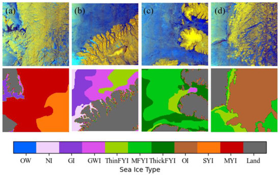 Figure 1. Cases of the visual similarity of different sea ice types in Sentinel-1 SAR images acquired on (a) 6 October 2019, (b) 19 October 2019, (c) 10 November 2019, (d) 5 January 2020. The first and second rows are RGB (R: HV, G: HH, B: HH/HV) SAR images and corresponding sea ice types derived from CIS sea ice charts, respectively. In this paper, the colors indicating differing sea ice types follow the World Meteorological Organization (WMO) standards. Abbreviations are: OW for open water, NI for new ice, GI for grey ice, GWI for grey-white ice, ThinFYI for thin first-year ice, MFYI for medium first-year ice, ThickFYI for thick first-year ice, OI for old ice, SYI for second-year ice, and MYI for multi-year ice.
- (2)
- In the field of computer vision, DL models designed for classification tasks are typically constructed using artificially balanced datasets, where each category has a roughly equal number of samples. Conversely, real-world datasets often exhibit class imbalance, as exemplified by the sea ice datasets utilized in this research. When dealing with such imbalanced datasets, common DL methods are not able to achieve outstanding classification accuracy. To illustrate this, we trained the ResNet-50 model [25] to classify sea ice types. The sea ice type distribution of the training dataset and the classwise F1-score of the test dataset are shown in Figure 2.
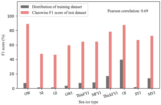 Figure 2. Comparison of the sea ice type distribution of the training dataset and the classwise F1-score of the test dataset.
Compared with other sea ice types, new ice (NI), grey ice (GI), grey-white ice (GWI), and second-year ice (SYI) occupy a very small part of the whole datasets. Accordingly, they have poor prediction accuracy. The strong Pearson correlation observed between data distribution and the F1-score suggests that the issue of class imbalance adversely impacts the performance of the model, particularly with respect to the minority classes.
To address the challenges outlined above, an end-to-end DL-based sea ice classification algorithm with Sentinel-1 SAR images is developed in this study. It can distinguish 10 sea ice types automatically. To classify similar sea ice types with close developmental stages, a spatio-temporal DL model—the Dynamic MLP—is used to learn temporal and spatial variation characteristics of sea ice. In order to mitigate the impact of the data imbalance problem on model performance, the dynamic curriculum learning (DCL) training strategy is applied to train the DL framework. Furthermore, a novel method is proposed to handle the effects of incidence angle, following the core idea of the Dynamic MLP model. Experimental results demonstrate that our proposed method outperforms the most advanced LSTM model. Meanwhile, the validity of the proposed approach for processing the data imbalance problem and incidence angle effects is also demonstrated by additional experiments.
The organization of this paper is delineated as follows. Section 2 introduces the study area and the data utilized. Section 3 outlines the methodologies employed in the research. The results are presented in Section 4, followed by a discussion in Section 5. Finally, Section 6 provides the conclusions drawn from the study.
2. Study Area and Data
2.1. Area of Interest
This research focuses on the Eastern and Western Canadian Arctic regions as the designated study area, aiming to encompass a diverse range of sea ice conditions. Collectively, these regions represent two of the five CIS regions (see Figure 3), where the CIS conducts extensive long-term monitoring of sea ice and generates digital operational sea ice charts.
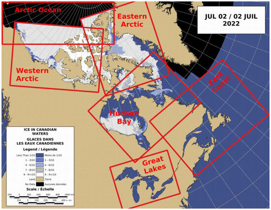
Figure 3.
Areas where sea ice service is provided by CIS. Red rectangular boxes indicate the monitoring regions. In this study, we focus on sea ice classification for the Western and Eastern Canadian Arctic regions.
The regions are subject to comprehensive monitoring by the Sentinel-1A and Sentinel-1B satellites, operating continuously both during daylight and nighttime hours. Both CIS sea ice charts and Sentinel-1 SAR imagery are used to develop our proposed automatic sea ice classification model. Further information regarding Sentinel-1 SAR imagery and sea ice charts is provided in Section 2.2 and Section 2.3, respectively. Based on CIS sea ice charts, the temporal and spatial variation characteristics of sea ice in the Eastern and Western Canadian Arctic are analyzed in Section 2.4. To train, validate, and evaluate our model, we construct a dataset following the methods given in Section 2.5.
2.2. Sentinel-1 SAR Imagery
The SAR images utilized in this research are derived from Sentinel-1 Level-1 Extra Wide Ground Range Detected (EW GRD) products. These images are captured in dual-polarized mode (HH/HV) and possess a medium spatial resolution of 40 m × 40 m, with a ground range coverage extending to 410 km. For the Eastern and Western Canadian Arctic, we collected 584 and 934 SAR images, respectively, which were spatially and temporally aligned with corresponding ice charts. This data collection occurred over the timeframe from 1 October 2019 to 30 September 2020. Among these images, 85% are used to train and validate the proposed algorithm and 15% are used to test our model.
2.3. Sea Ice Charts
In this study, the CIS Arctic regional sea ice charts serve as the reference standard. These charts are produced by specialists in ice forecasting, who utilize a combination of manual interpretation of satellite imagery, visual observations from maritime vessels and aircraft, as well as meteorological and oceanographic data. To ensure comprehensive coverage of the designated area for each chart, satellite data are gathered over multiple days. The resulting charts are made available in digital shapefile format, specifically encoded in SIGRID-3.
The charts present estimates of ice concentration measured in tenths, alongside the stages of ice development and the various forms of ice. The ice data is encoded in accordance with the standards set by the World Meteorological Organization (WMO). In this research, we categorize sea ice into 10 distinct types based on their developmental stages, which include open water (OW), new ice (NI), grey ice (GI), grey-white ice (GWI), thin first-year ice (ThinFYI), medium first-year ice (MFYI), thick first-year ice (ThickFYI), old ice (OI), second-year ice (SYI), and multi-year ice (MYI). Additionally, the charts incorporate a land mask, allowing for the estimation of land locations. The definitions of the sea ice terminology utilized in this study adhere to the guidelines established by Environment and Climate Change Canada (ECCC) protocol. The thickness of the ice types and their corresponding WMO codes are detailed in Table 1.

Table 1.
Sea ice type definition and code.
2.4. Temporal and Spatial Variation Characteristics of Sea Ice
Based on CIS sea ice charts, we first analyzed the temporal and spatial variation characteristics of sea ice in the Eastern and Western Canadian Arctic. The results are given in Appendix A. As shown in Figure A1 and Figure A2, sea ice in the Eastern and Western Canadian Arctic has rather obvious temporal variation trends: the growth and evolution of sea ice are progressive and periodic. For example, in the Western Canadian Arctic, OW begins to freeze up and NI, GI, GWI form in late October (see Figure A1). By the beginning of December, most of the newly formed sea ice turns into ThinFYI. Waters of the Western Arctic are completely ice-covered by late December. As sea ice grows, it becomes thicker. In the following summer, by August, the dominant sea ice type becomes OI and partially ThickFYI. Overall, in summertime, sea ice in waters adjacent to Northern Canada has entered the melting phase. However, during summer, only a relatively small area of the sea ice is completely melted in the Western Canadian Arctic. The maximum area of OW occurs in early October, and at the same time, OI becomes SYI and MYI.
To quantitatively describe the characteristics of sea ice growth and changes over time, we calculated the transition probability of sea ice, transferring from one type to the others during a one-week interval. Transition probability is a concept in probability theory and statistics, particularly in the context of Markov chains and stochastic processes. It represents the probability of moving from one state to another state in a system that changes over time. In a Markov chain, the transition probability is the probability of transitioning from state to state in one time step. These probabilities are often represented by a transition matrix, where the entry in the -th row and -th column of the matrix gives the probability of moving from state to state .
The statistical results are shown in Figure 4, highlighting the ‘transition law’ of sea ice types. For a given week, the sea ice type is most likely to remain unchanged or progress to the next closest developmental stage in the following week. Additionally, the spatial distribution of sea ice varies significantly across regions. For example, the dominant sea ice types in the Western Arctic are first-year ice (FYI, including ThinFYI, MFYI, and ThickFYI), MYI, and OI, while the dominant sea ice type in the Eastern Arctic is FYI. In conclusion, sea ice exhibits unique temporal transition patterns and varying spatial distribution characteristics, which can be leveraged to differentiate between similar types of sea ice.
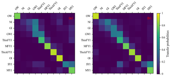
Figure 4.
Statistical results of temporal variation characteristics of different sea ice types in: (a) Western Arctic and (b) Eastern Arctic.
2.5. Dataset Construction
Before developing the model, we preprocess the data and construct suitable datasets to train, validate, and test our model. For SAR image processing, radiometric corrections and the elimination of thermal noise are conducted on both HH- and HV-polarized SAR images in order to obtain normalized radar cross section (NRCS) values and , according to the coefficients provided in the calibration file. Subsequently, a 10 × 10 down-sampling is performed using the boxcar average method to reduce speckle noise and computational load. This results in a pixel spacing of 400 m. The values and are then converted to dB and normalized by applying the Z-score method, which standardizes data based on their mean and standard deviation. The multimodal information is normalized to a range of (−1, 1), including incidence angles, longitudes, latitudes, and dates. Finally, we use sea ice charts to annotate the SAR images. The sea ice charts are first matched to the SAR images, within 3 days prior to the chart dates, and are then interpolated to the SAR image grids using nearest-neighbour interpolation.
For dataset construction, all SAR images are divided into small samples, in number 30 × 30 (each is 12 km × 12 km), which are labeled by the dominate sea ice type in each. The selected size is deemed appropriate, as each polygon in the sea ice charts, representing an area with uniform sea ice characteristics, varies from several kilometers to several tens of kilometers, contingent upon the subjective assessments of the ice analyst. The labeled samples within the training dataset are subsequently divided into training and validation datasets at a ratio of 9:1.
3. Methods
3.1. Framework of the Dynamic MLP Model
According to CIS charts, sea ice can be divided into 10 types based on developmental stage. Different sea ice types have very similar characteristics in SAR images, especially those at close developmental stages. Hence, the sea ice classification task is categorized as a fine-grained image classification exercise, which is a challenging task that involves identifying fine categories of species or objects. In contrast to conventional image classification, fine-grained image classification presents significant challenges in distinguishing different objects or species that have very similar appearances. These are quite difficult to differentiate by images alone. To deal with this problem, the Dynamic MLP has been proposed for fine-grained image classification. By incorporating additional spatio-temporal information, the model has proven to be superior to previous methods [26]. Consequently, this research examines the capacity of Dynamic MLP to categorize different types of sea ice that exhibit similar visual characteristics.
The Dynamic MLP is a bilateral-path framework, as shown in Figure 5. It contains two branches (i.e., the SAR image branch and spatio-temporal branch) and consists of several CNN and MLP blocks. Initially, SAR image patches and their corresponding spatio-temporal information are input to their respective branches simultaneously.
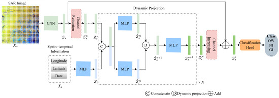
Figure 5.
Overall architecture of Dynamic MLP. It contains two branches for extracting features from the SAR image and corresponding spatio-temporal information, respectively. The core structure of Dynamic MLP is a dynamic projection block, denoted as “D”, which updates the image representation recursively by N times, according to the weights generated from spatio-temporal features.
In the SAR image branch, a CNN block is employed to extract representations from SAR images. At the same time, the spatio-temporal features are derived through the MLP block. Next, a dynamic projection block is employed to assign analogous image features to distinct locations within the feature space. The image features are updated by the dynamic projection block, based on the adaptive weights derived from spatio-temporal features. The essence of this dynamic projection process is related to high-dimensional interactions between image representations and spatio-temporal features. Finally, the enhanced image features are used to make predictions.
To be more specific, given the input image , its image features can be extracted via the CNN block. To reduce memory usage and save computation time, image features are transformed to with lower dimensions, by a channel-reduction layer.
Simultaneously, the spatio-temporal information is normalized to (−1, 1) and concatenated channel-wise:
where represents channel-wise concatenation. The spatio-temporal information is mapped to by sine–cosine encoding:
Then, the spatio-temporal branch takes additional location and time information, , as inputs, and generates the spatio-temporal features through the MLP block.
Next, the image and spatio-temporal features are fused by the dynamic projection block. Taking and as initial inputs, the image features are dynamically projected to the spatio-temporal feature space. After N recursive projections, the improved image representations are obtained. Then, a channel increasing operation is performed to keep the shape of and original image features consistent. Finally, and are combined via a ‘skip connection’ to make final predictions.
Detailed structures of the CNN block, the MLP block, and the dynamic projection block are given as follows.
3.1.1. The CNN Block
The Residual Convolutional Network (ResNet) [25] is recognized as a foundational model within the realm of Convolutional Neural Networks (CNNs) employed for image classification tasks. The key component of the ResNet model is the residual block with identity shortcut connections, as shown in Figure 6.
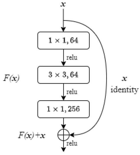
Figure 6.
Residual block.
Let x represent the input vector and H(x) denote an underlying mapping that is to be approximated through multiple stacked convolutional layers. These layers aim to approximate a residual function , thereby transforming the original mapping into the form . It is generally more feasible to approximate the residual mapping than to directly fit the original mapping. The expression of can be implemented through shortcut connections, which execute identity mapping by bypassing one or more layers. Consequently, the residual block is defined as follows:
where y is the output vector of the layers, are layer weights and is a linear projection matrix. denotes the residual function to be learned.
In this study, we used a 50-layer ResNet model to extract SAR image features. The comprehensive architecture of ResNet is presented in Table 2. Residual blocks are shown in brackets, with the number of blocks stacked. Batch normalization (BN) and a rectified linear unit (ReLU) activation function are applied subsequent to each convolutional operation.
Table 2.
Structure of the ResNet model.
3.1.2. The MLP Block
The MLP block for spatio-temporal feature extraction is a residual MLP, and the remaining MLP blocks are common fully connected layers. As illustrated in Figure 7, the residual MLP consists of several linear layers, ReLU layers, and residual layers [27]. The residual layer is a derivative of the residual block. The input of the residual layer is skip-connected with the output of the last RuLU layer, for residual learning.
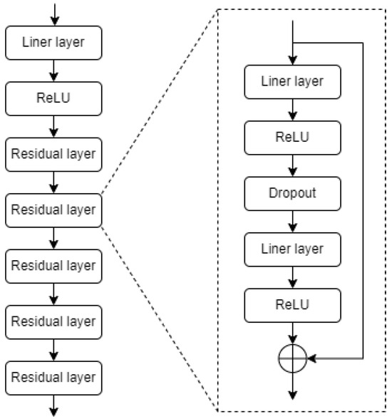
Figure 7.
Structure of the MLP block.
3.1.3. The Dynamic Projection Block
The dynamic projection block is an iterable structure, which enhances the quality of image representations adaptively, with the help of spatio-temporal features. Since the image representations and spatio-temporal features can provide complementary information, they can jointly generate better conditional weights during the projection process.
Specifically, as shown in Figure 5, the image features and spatio-temporal features are combined in a channel-wise manner to serve as the input of the dynamic projection block. Then, two identical MLP blocks are used to learn the interaction between them. New image features and spatio-temporal features are denoted as and , respectively, where n indicates the current update stage and . Next, the image features are projected to the spatio-temporal feature space. The projection process is shown in Figure 8. The weights of the dynamic projector are calculated according to the spatio-temporal features:
where converts 1-d features to a 2-d feature and indicates the fully connected layer.
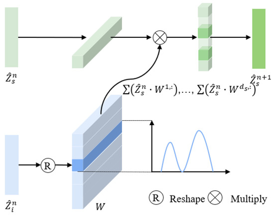
Figure 8.
Overview of the dynamic projection process, indicated as “D” in Figure 5.
After the dynamic projection, the image features can be written as:
where denotes the feature channels. The following MLP block can be expressed as:
where represents layer normalization.
The above dynamic projection process is iterated N times. The enhanced image representations will be used for the final predictions.
3.2. Framework of Dynamic Curriculum Learning Training
The notion of curriculum learning (CL) was initially introduced by Bengio et al. [28]. CL represents a training methodology that systematically instructs machine learning models by presenting data in a structured sequence, progressing from simpler to more complex examples. This is inspired by human learning, where curricula are arranged from easy levels to hard levels during human education. CL has been demonstrated to enhance the generalization capabilities and convergence rates of models in the domains of computer vision and natural language processing [29,30]. In the field of sea ice remote sensing, CL has been applied to improve the precision of sea ice concentration estimation in the marginal ice zone (MIZ) [31]. It has also been successfully applied in class-imbalanced classification tasks [32]. In this study, the dynamic curriculum learning (DCL) [32] framework is adopted to address the issue of class imbalance in sea ice classification. It consists of two-level curriculum schedulers, including a sampling scheduler and a loss scheduler.
3.2.1. Sampling Scheduler
The function of the sampling scheduler is to dynamically modify the data distribution within a single batch, transitioning from an imbalanced to a balanced state, as well as from simpler to more challenging instances, throughout the training phase. For a given training set, the jth element of the data distribution can be defined as the ratio of the number of the jth class samples to the number of the least class samples. When these elements are arranged in ascending order, the following results are obtained:
where is the number of classes, is the number of samples in class i, and is the number of the least class samples.
Then, the sampling scheduler function is used to adapt the target data distribution in one batch dynamically. It is defined by a convex function, shown in Figure 9:
where l and L represent current epoch and total training epochs, respectively.
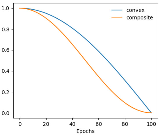
Figure 9.
Scheduler functions.
Initially, the target data distribution at epoch 0 in each batch is set to , characterized by an imbalanced distribution. As the training process continues, this distribution progressively evolves into a balanced state, with the help of the sampling scheduler:
According to target data distribution , samples of each class are selected dynamically in different epochs during the training stage. At the initial epoch, means the target data distribution equals the training set distribution, which is imbalanced. At the last epoch, , which indicates that the target data distribution is balanced; namely, the number of each class sample equals .
3.2.2. Loss Scheduler
Based on the sampling scheduler, the dynamic selective learning (DSL) loss is used to better learn from the minority class and is defined as follows:
where M, N, and are the number of classes, the batch size, and the number of jth class samples at the current batch, respectively.
and are prediction labels and ground truth labels, respectively. is the weight function for class j, and is defined as follows:
where is the target distribution of class j at the current epoch and is the jth class distribution at the current batch before sampling. If , the jth class is a majority class. We sample percentage of jth class samples with weight 1, and the remaining have weight 0. Otherwise, the jth class is a minority class and a larger weight is used. In short, the weight for the minority class is increasing dynamically with training.
In addition to the DSL loss, the triplet loss from the metric learning is also used to better discriminate similar samples with difficult or ‘hard’ mining. We define hard samples as wrongly predicted samples with high confidence. We characterize ‘easy’ anchors as minority samples that are accurately predicted with a high degree of confidence. Subsequently, triplet pairs can be constructed using these easy anchors, along with hard positive and negative samples, which are defined as follows:
where is the margin of class j and represents the feature distance between two samples. and refer to positive and negative samples, respectively. denotes easy samples in the minority class j. is the number of triplet pairs.
Combining and , the loss scheduler is defined as:
where and are the advanced self-learning point and self-learning ratio, respectively.
3.3. Evaluation Metrics
Due to the significant imbalance present in the sea ice datasets, the evaluation metrics chosen for this study include the classwise F1-score, the micro-average F1-score (), and the macro-average F1-score () [33]. The F1-score is defined as the harmonic mean of precision and recall:
where and are precision and recall, respectively.
Based on the confusion matrix, and can be computed as follows:
where , , and represent true positives, false positives, and false negatives, respectively. According to the above definitions, precision denotes the correct proportion of positive identifications, while recall denotes the correctly identified proportion of actual positives. They are a pair of contradictory performance evaluation metrics. High precision means low recall and vice versa. The F1-score represents a metric that effectively reconciles the trade-off between precision and recall.
is defined as:
where
where , , , and denote true positives, false positives, false negatives, and F1-score of the -th class, respectively. is the class number. represents the mean of the F1-scores calculated for each class, thereby highlighting the significance of each individual class and placing greater emphasis on those that are less frequently occurring.
is defined as:
where
Compared with , treats each sample equally, equivalent to overall accuracy (OA) numerically.
3.4. Implementation Details
All models are developed utilizing the PyTorch framework. The training of these models is conducted using the stochastic gradient descent (SGD) optimizer, configured with a momentum of 0.9, a weight decay of 10−4, a batch size of 512, and a cosine learning rate schedule that progressively decreases from 0.04 to 0. To mitigate the potential for overfitting and enhance the generalization capabilities of the models, we employ various data augmentation techniques on the training dataset, including random horizontal flips, random vertical flips, and random rotations of 90°, 180°, and 270° [34]. Each model undergoes training for a total of 90 epochs. Additionally, we implement a warm-up strategy [35] during the initial two epochs, which involves incrementally increasing the learning rate from a lower value to a higher one. This helps the model gradually adapt to the characteristics of the dataset, reducing oscillations and instability during training.
4. Results
4.1. Performance Comparison of Sea Ice Classification Models
The LSTM model is selected as the baseline because it is the state-of-the-art DL model, known for its ability to discriminate similar sea ice types [24]. In this section, we evaluate the classification accuracy of three DL methods: the LSTM, the Dynamic MLP, and our proposed Dynamic MLP + DCL model.
The overall performance evaluation results are shown in Table 3. Compared with the LSTM model, which only considers temporal information, the classification accuracy of the Dynamic MLP model achieves great improvement by making use of both spatial and temporal information. Furthermore, the Dynamic MLP model, trained with the DCL framework, performs best among the three models. Specifically, in terms of the performance indicators, the Dynamic MLP model outperforms the LSTM method by 10.58% (relative difference) in and 15.71% in , while the Dynamic MLP + DCL method achieves 18.15% and 27.61% performance gains in and over the LSTM model, respectively.
Table 3.
Performance comparison among different classification models.
Figure 10 presents the classwise F1-scores of the three DL models. The results clearly indicate that data imbalance has a significant negative effect on model performance, over the minority classes. Compared to the LSTM model, the Dynamic MLP model substantially improves the classification accuracy for ThinFYI, MFYI, OI, and MYI, but shows decreased prediction accuracy for other sea ice types to varying degrees. In contrast to the Dynamic MLP model, our proposed Dynamic MLP + DCL method can further improve the classification accuracy of all sea ice types, especially the minority classes, such as GI, GWI, ThinFYI, MFYI, ThickFYI, SYI, and MYI. Therefore, our method can mitigate the impact of data imbalance on prediction performance.
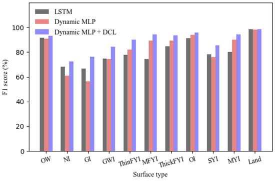
Figure 10.
Classwise F1-score for three DL methods: LSTM, Dynamic MLP, and Dynamic MLP + DCL.
Figure 11 shows the sea ice classification results for SAR images using the three methods. According to the ice chart, the sea ice types in the SAR image (Figure 11a) are mainly GWI, ThinFYI, and MYI. The LSTM model failed to identify GWI, misclassifying it as ThinFYI and MYI. The Dynamic MLP model is able to identify some GWI, but other GWI areas are misclassified as MYI. Additionally, the Dynamic MLP model fails to effectively distinguish between ThinFYI and GWI. In comparison, the Dynamic MLP + DCL model can effectively recognize these three types of sea ice, with only a small proportion of GWI being misclassified as ThinFYI.
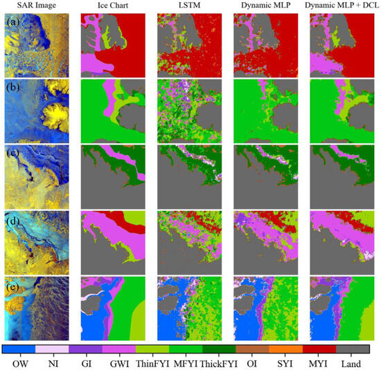
Figure 11.
Cases of classification results for Sentinel-1 SAR images acquired on (a) 27 October 2019, (b) 15 February 2020, (c) 3 April 2020, (d) 17 November 2019 and (e) 11 January 2020. The columns from left to right represent RGB (R: HV, G: HH, B: HH/HV) SAR imageries, ice charts, and classification results from LSTM, Dynamic MLP, and Dynamic MLP + DCL.
In the SAR image in Figure 11b, the sea ice types are GWI, ThinFYI, and MFYI. The LSTM model fails to distinguish between these types. The Dynamic MLP model correctly identifies MFYI and a small portion of GWI but misclassifies ThinFYI as MFYI. The Dynamic MLP + DCL model effectively distinguishes the three sea ice types, with only a small portion of the GWI area misjudged as ThinFYI or MFYI.
In the SAR image in Figure 11c, the sea ice types are GWI and ThickFYI. All three models can correctly classify ThickFYI. The LSTM model and Dynamic MLP model have poor ability to identify GWI, while the Dynamic MLP + DCL model can correctly predict part of GWI.
Typical sea ice types in the SAR image in Figure 11d are GWI, MYI, and ThinFYI, distributed in a banded pattern. The LSTM model cannot distinguish them effectively, but both the Dynamic MLP model and the Dynamic MLP + DCL model can predict them well, and the classification result of the Dynamic MLP + DCL model is significantly better than that of the Dynamic MLP model.
The SAR image in Figure 11e is located in the MIZ, covering a variety of sea ice types: OW, NI, GI, GWI, ThinFYI, and MFYI. The three models are all able to correctly identify the boundary between sea ice and OW. The LSTM model and the Dynamic MLP model fail to distinguish between ThinFYI and MFYI, and the former model cannot identify GI and GWI in the MIZ effectively. The Dynamic MLP model and the Dynamic MLP + DCL model can distinguish parts of GI and GWI correctly in the MIZ. In general, the Dynamic MLP + DCL model outperforms the other models in accurately classifying sea ice types within the MIZ.
In summary, compared with the LSTM model, the Dynamic MLP model can effectively distinguish between sea ice types with similar developmental stages, such as first year ice of different thicknesses. On the basis of the Dynamic MLP model, our proposed Dynamic MLP + DCL method can further improve the classification accuracy of the minority sea ice types, and it also performs well in the complex MIZ.
4.2. Influence of Incidence Angle Dependence
It is well known that the NRCSs of sea ice have a strong incidence angle dependence [36,37,38,39]. For Sentinel-1 EW images, with a large incidence angle range (19–47°), varying NRCS values will confuse image interpretation. Therefore, it is necessary to study the effect of incidence angle dependence on sea ice classification.
At present, there are two primary methods to deal with this dependence relationship, which can be summarized as follows:
- (1)
- The NRCS can be normalized through incidence angle correction for all swath ranges [11,12,14,16,21,40]. The incidence angle dependence of OW and sea ice NRCS in HH polarization is illustrated in Figure 12. The NRCS of OW and sea ice is a linear function of the incidence angle, with the incidence angle dependence for OW being significantly higher than for sea ice. This is consistent with previous studies [36,37,38,39]. Although we can calculate the dependence relationship for OW and each sea ice type by simple linear fitting, it is difficult to determine the total compensation because the surface type is not known a priori. As a result, the incidence angle influence has not been considered in some studies [19,22,24].
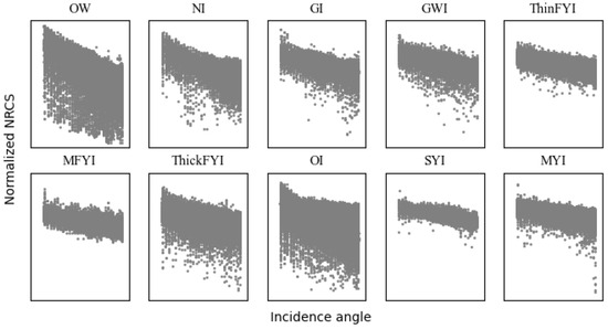 Figure 12. Incidence angle dependence of OW and sea ice NRCS in HH polarization.
 - (2)
- The incidence angle can be considered as an additional input channel, with the same two-dimensional size as the input patches [17]. Specifically, the input of the SAR image branch consists of three channels: , , and the incidence angles. This method is not optimal because no textural information is contained in incidence angles. This will also significantly increase the computational load.Following the core idea of dynamic MLP, we propose the third method:
- (3)
- The averaged incidence angle of each sample is utilized as an additional input of the spatio-temporal branch. By projecting similar sea ice features to different incidence angles, the sea ice classification ability of our model can be further enhanced.
In this study, we evaluate the latter two methods in detail, with the performance evaluation results shown in Table 4. Both methods (2) and (3) improve the classification accuracy of sea ice, with method (3) outperforming method (2), further proving the validity of our proposed model architecture. However, in general, the effect of incidence angle dependence on model performance is minimal. This may be due to the model’s ability to learn the incidence angle dependence from the SAR images to a certain extent.
Table 4.
Performance comparison between two different incidence angle handling methods.
5. Discussion
5.1. Advantages
The approach presented in this article, i.e., training the Dynamic MLP model with the DCL method, is able to identify 10 sea ice types with high accuracy. Compared to the classic LSTM method, which can only extract time variation features of sea ice, the Dynamic MLP model has a powerful capability to learn both the temporal and the geospatial distribution characteristics of sea ice. The benefit of its unique and elegant design, where a dynamic projection block is used to map similar SAR image features to different positions in the spatio-temporal feature space, is that the Dynamic MLP model is able to identify sea ice types with closely related developmental stages. Furthermore, with the help of the DCL training strategy, the classification accuracy of the Dynamic MLP model in predicting the minority ice types is improved greatly.
Further, the Dynamic MLP model demonstrates superior computational efficiency in comparison with the LSTM model, as illustrated in Table 5. The training durations for the Dynamic MLP model and the Dynamic MLP + DCL model are approximately 1/5 and 1/3, respectively, of the training time required for the LSTM model. Additionally, the inference speed of the Dynamic MLP model is seven times faster than that of the LSTM model.
Table 5.
Computational efficiency comparison among different classification models.
5.2. Limitations and Future Work
Some limitations remain concerning data sources, dataset construction, and model architecture. In this study, our method was developed based on Sentinel-1 C-band SAR images. The effectiveness of this methodology should be assessed through the analysis of additional SAR images obtained from a range of satellites and frequency bands, including but not limited to Radarsat-2 and TerraSAR-X.
In this study, the CIS sea ice charts serve as the reference standard for model training and evaluation. However, they assign a singular label to extensive spatial areas characterized by uniform ice properties. Consequently, the ice type at a specific location within these regions may not correspond to the designated label. For example, these charts do not adequately represent small-scale features such as ice floes and openings within the ice cover. Additionally, given that our classification approach was implemented at the patch level, it is unavoidable that certain pixel patches may contain a mixture of sea ice types in the actual classification of SAR images. Furthermore, it is important to note that sea ice charts may exhibit biases stemming from the subjective interpretations of ice experts. To evaluate the effect of label errors on model performance quantitatively, some errors were introduced into the training labels manually. To be specific, we randomly selected a certain proportion of samples and replaced their labels with those of types at closely related developmental stages. This approach is justified, as differentiating between sea ice types that are at comparable stages of development is inherently difficult. Consequently, this methodology allows us to indirectly evaluate the impact of label errors on model performance. As illustrated in Table 6, the performance of all models exhibits a decline in response to an increasing proportion of incorrect labels. When 10% of the samples have label errors, the Dynamic MLP + DCL model is able to maintain a relatively high level of prediction accuracy. However, once the proportion of erroneous labels exceeds 20%, the impact of label errors on model performance becomes significant and cannot be ignored.
Table 6.
Performance comparison among different classification models.
To address the impact of label errors on model performance, we consider noise label learning (NNL) [41] to be a feasible solution. NNL is a subfield of machine learning that focuses on training models in the presence of noisy or incorrect labels in the training data. In real-world scenarios, labeled datasets, such as the sea ice datasets used in this study, often contain errors due to human annotation mistakes, automatic labeling processes, or ambiguous data. NNL aims to develop algorithms and techniques that can robustly learn from such imperfect data, improving model performance and generalization. In the future, we plan to investigate several NNL approaches, such as noise-tolerant algorithms, noise detection and correction methods, and semi-supervised and self-supervised learning techniques.
6. Conclusions
There are two major challenges in DL-based sea ice classification using SAR images: (1) sea ice types at similar developmental stages exhibit similar image features in SAR images, and (2) the distribution of sea ice datasets is highly imbalanced, leading to poor classification accuracy for minority classes. To address these challenges, we propose the Dynamic MLP + DCL method. The Dynamic MLP model is able to effectively distinguish up to 10 sea ice types by integrating SAR image features with the spatio-temporal distribution characteristics of sea ice. On this basis, the DCL training framework is used to train the Dynamic MLP, further addressing the issue of data imbalance. Compared with the current state-of-the-art LSTM model, our method has significantly improved the classification accuracy of sea ice, especially minority classes. In addition, we quantitatively evaluate the impact of incidence angle dependence on model performance. Experimental results show that our proposed incidence angle processing method can further improve the model’s classification accuracy. However, overall, incidence angle dependence has minimal impact on model performance, likely because the model has the ability to learn this incidence angle dependence from the SAR images by itself.
Author Contributions
Conceptualization, L.Z. and W.Z.; methodology, L.Z. and Y.Z.; software, L.Z., Y.Z., and C.J.; validation, L.Z., Y.Z., and C.J.; formal analysis, W.Z.; investigation, L.Z.; resources, W.Z.; data curation, L.Z.; writing—original draft preparation, L.Z.; writing—review and editing, W.Z., B.L., and F.L.; visualization, L.Z.; supervision, W.Z.; project administration, W.Z.; funding acquisition, W.Z. All authors have read and agreed to the published version of the manuscript.
Funding
This research was funded by the National Key R&D Program of China under grant number 2021YFC2803302 and the National Natural Science Foundation of China project under grant number 42075011.
Data Availability Statement
The Sentinel-1 SAR images are available from NASA’s Alaska Satellite Facility Distributed Active Archive Center (ASF DAAC) at https://search.asf.alaska.edu/#/ (accessed on 2 December 2024). CIS Arctic regional sea ice charts can be downloaded from the National Snow and Ice Data Center (NSIDC) at https://nsidc.org/data/g02171/versions/1 (accessed on 2 December 2024).
Acknowledgments
The authors would like to express their sincere gratitude to the anonymous reviewers for their valuable comments and suggestions, which have greatly improved the quality of this manuscript.
Conflicts of Interest
The authors declare no conflicts of interest.
Appendix A
Figure A1 and Figure A2 show the spatial and temporal distribution of sea ice in the Western and Eastern Canadian Arctic during October 2019 to September 2020, respectively.
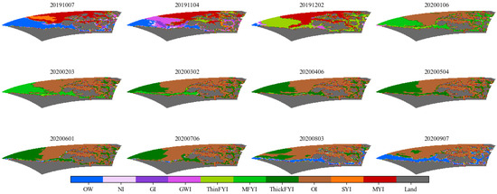
Figure A1.
The spatial and temporal distribution of sea ice in Western Canadian Arctic during October 2019 to September 2020.
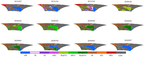
Figure A2.
The spatial and temporal distribution of sea ice in Eastern Canadian Arctic during October 2019 to September 2020.
References
- Comiso, J.C.; Parkinson, C.L.; Gersten, R.; Stock, L. Accelerated decline in the Arctic sea ice cover. Geophys. Res. Lett. 2008, 35, L01703. [Google Scholar] [CrossRef]
- Liu, Z.; Risi, C.; Codron, F.; He, X.; Poulsen, C.J.; Wei, Z.; Chen, D.; Li, S.; Bowen, G.J. Acceleration of western Arctic sea ice loss linked to the Pacific North American pattern. Nat. Commun. 2021, 12, 1519. [Google Scholar] [CrossRef] [PubMed]
- Tivy, A.; Howell, S.E.; Alt, B.; McCourt, S.; Chagnon, R.; Crocker, G.; Carrieres, T.; Yackel, J.J. Trends and variability in summer sea ice cover in the Canadian Arctic based on the Canadian Ice Service Digital Archive, 1960–2008 and 1968–2008. J. Geophys. Res. Ocean. 2011, 116, C03007. [Google Scholar] [CrossRef]
- Wang, Z.; Li, Z.; Zeng, J.; Liang, S.; Zhang, P.; Tang, F.; Chen, S.; Ma, X. Spatial and temporal variations of Arctic sea ice from 2002 to 2017. Earth Space Sci. 2020, 7, e2020EA001278. [Google Scholar] [CrossRef]
- Cai, Q.; Wang, J.; Beletsky, D.; Overland, J.; Ikeda, M.; Wan, L. Accelerated decline of summer Arctic sea ice during 1850–2017 and the amplified Arctic warming during the recent decades. Environ. Res. Lett. 2021, 16, 034015. [Google Scholar] [CrossRef]
- Xie, T.; Perrie, W.; Fang, H.; Zhao, L.; Yu, W.; He, Y. Spatial and temporal variability of sea ice deformation rates in the Arctic Ocean observed by RADARSAT-1. Sci. China Earth Sci. 2017, 60, 858–865. [Google Scholar] [CrossRef]
- Rodriguez-Alvarez, N.; Holt, B.; Jaruwatanadilok, S.; Podest, E.; Cavanaugh, K.C. An Arctic sea ice multi-step classification based on GNSS-R data from the TDS-1 mission. Remote Sens. Environ. 2019, 230, 111202. [Google Scholar] [CrossRef]
- Yan, Q.; Huang, W. Sea Ice Remote Sensing Using GNSS-R: A Review. Remote Sens. 2019, 11, 2565. [Google Scholar] [CrossRef]
- Yan, Q.; Huang, W. Sea Ice Sensing From GNSS-R Data Using Convolutional Neural Networks. IEEE Geosci. Remote. Sens. Lett. 2018, 15, 1510–1514. [Google Scholar] [CrossRef]
- Zhu, Y.; Tao, T.; Li, J.; Yu, K.; Wang, L.; Qu, X.; Li, S.; Semmling, M.; Wickert, J. Spaceborne GNSS-R for Sea Ice Classification Using Machine Learning Classifiers. Remote Sens. 2021, 13, 4577. [Google Scholar] [CrossRef]
- Liu, H.; Guo, H.; Zhang, L. SVM-based sea ice classification using textural features and concentration from RADARSAT-2 dual-pol ScanSAR data. IEEE J. Sel. Top. Appl. Earth Obs. Remote Sens. 2015, 8, 1601–1613. [Google Scholar] [CrossRef]
- Zakhvatkina, N.; Korosov, A.; Muckenhuber, S.; Sandven, S.; Babiker, M. Operational algorithm for ice–water classification on dual-polarized RADARSAT-2 images. Cryosphere 2017, 11, 33–46. [Google Scholar] [CrossRef]
- Zhang, L.; Liu, H.; Gu, X.; Guo, H.; Chen, J.; Liu, G. Sea ice classification using TerraSAR-X ScanSAR data with removal of scalloping and interscan banding. IEEE J. Sel. Top. Appl. Earth Obs. Remote Sens. 2019, 12, 589–598. [Google Scholar] [CrossRef]
- Park, J.-W.; Korosov, A.A.; Babiker, M.; Won, J.-S.; Hansen, M.W.; Kim, H.-C. Classification of sea ice types in Sentinel-1 synthetic aperture radar images. Cryosphere 2019, 14, 2629–2645. [Google Scholar] [CrossRef]
- Fredensborg Hansen, R.M.; Rinne, E.; Skourup, H. Classification of Sea Ice Types in the Arctic by Radar Echoes from SARAL/AltiKa. Remote Sens. 2021, 13, 3183. [Google Scholar] [CrossRef]
- Boulze, H.; Korosov, A.; Brajard, J. Classification of sea ice types in Sentinel-1 SAR data using convolutional neural networks. Remote Sens. 2020, 12, 2165. [Google Scholar] [CrossRef]
- Khaleghian, S.; Ullah, H.; Kræmer, T.; Hughes, N.; Eltoft, T.; Marinoni, A. Sea ice classification of SAR imagery based on convolution neural networks. Remote Sens. 2021, 13, 1734. [Google Scholar] [CrossRef]
- Zhang, J.; Zhang, W.; Hu, Y.; Chu, Q.; Liu, L. An improved sea ice classification algorithm with Gaofen-3 dual-polarization SAR data based on deep convolutional neural networks. Remote Sens. 2022, 14, 906. [Google Scholar] [CrossRef]
- Lyu, H.; Huang, W.; Mahdianpari, M. Eastern Arctic Sea Ice Sensing: First Results from the RADARSAT Constellation Mission Data. Remote Sens. 2022, 14, 1165. [Google Scholar] [CrossRef]
- Zhao, L.; Xie, T.; Perrie, W.; Yang, J. Deep Learning-Based Sea Ice Classification with Sentinel-1 and AMSR-2 Data. IEEE J. Sel. Top. Appl. Earth Obs. Remote Sens. 2023, 16, 5514–5525. [Google Scholar] [CrossRef]
- Wang, Y.-R.; Li, X.-M. Arctic sea ice cover data from spaceborne synthetic aperture radar by deep learning. Earth Syst. Sci. Data 2021, 13, 2723–2742. [Google Scholar] [CrossRef]
- Ren, Y.; Li, X.; Yang, X.; Xu, H. Development of a dual-attention U-Net model for sea ice and open water classification on SAR images. IEEE Geosci. Remote. Sens. Lett. 2022, 19, 4010205. [Google Scholar] [CrossRef]
- Zhao, L.; Xie, T.; Perrie, W.; Yang, J. Sea Ice Detection from RADARSAT-2 Quad-Polarization SAR Imagery Based on Co- and Cross-Polarization Ratio. Remote Sens. 2024, 16, 515. [Google Scholar] [CrossRef]
- Song, W.; Li, M.; Gao, W.; Huang, D.; Ma, Z.; Liotta, A.; Perra, C. Automatic Sea-Ice Classification of SAR Images Based on Spatial and Temporal Features Learning. IEEE Trans. Geosci. Remote Sens. 2021, 59, 9887–9901. [Google Scholar] [CrossRef]
- He, K.; Zhang, X.; Ren, S.; Sun, J. Deep residual learning for image recognition. In Proceedings of the 2016 IEEE Conference on Computer Vision and Pattern Recognition (CVPR), Las Vegas, NV, USA, 27–30 June 2016; pp. 770–778. [Google Scholar]
- Yang, L.; Li, X.; Song, R.; Zhao, B.; Tao, J.; Zhou, S.; Liang, J.; Yang, J. Dynamic MLP for Fine-Grained Image Classification by Leveraging Geographical and Temporal Information. In Proceedings of the IEEE/CVF Conference on Computer Vision and Pattern Recognition (CVPR), New Orleans, LA, USA, 18–24 June 2022; pp. 10945–10954. [Google Scholar]
- Mac Aodha, O.; Cole, E.; Perona, P. Presence-only geographical priors for fine-grained image classification. In Proceedings of the 2019 IEEE/CVF International Conference on Computer Vision (ICCV), Seoul, Republic of Korea, 27 October–2 November 2019; pp. 9596–9606. [Google Scholar]
- Bengio, Y.; Louradour, J.; Collobert, R.; Weston, J. Curriculum learning. In Proceedings of the 26th Annual International Conference on Machine Learning, Montreal, QC, Canada, 14–18 June 2009; pp. 41–48. [Google Scholar]
- Soviany, P.; Ionescu, R.T.; Rota, P.; Sebe, N. Curriculum learning: A survey. Int. J. Comput. Vision 2022, 130, 1526–1565. [Google Scholar] [CrossRef]
- Wang, X.; Chen, Y.; Zhu, W. A survey on curriculum learning. IEEE Trans. Pattern Anal. Mach. Intell. 2021, 44, 4555–4576. [Google Scholar] [CrossRef]
- Radhakrishnan, K.; Scott, K.A.; Clausi, D.A. Sea Ice Concentration Estimation: Using Passive Microwave and SAR Data With a U-Net and Curriculum Learning. IEEE J. Sel. Top. Appl. Earth Obs. Remote Sens. 2021, 14, 5339–5351. [Google Scholar] [CrossRef]
- Wang, Y.; Gan, W.; Yang, J.; Wu, W.; Yan, J. Dynamic curriculum learning for imbalanced data classification. In Proceedings of the IEEE/CVF International Conference on Computer Vision, Seoul, Republic of Korea, 27 October–2 November 2019; pp. 5017–5026. [Google Scholar]
- Masolele, R.N.; De Sy, V.; Herold, M.; Marcos, D.; Verbesselt, J.; Gieseke, F.; Mullissa, A.G.; Martius, C. Spatial and temporal deep learning methods for deriving land-use following deforestation: A pan-tropical case study using Landsat time series. Remote Sens. Environ. 2021, 264, 112600. [Google Scholar] [CrossRef]
- Shorten, C.; Khoshgoftaar, T.M. A survey on image data augmentation for deep learning. J. Big Data 2019, 6, 1–48. [Google Scholar] [CrossRef]
- Goyal, P.; Dollár, P.; Girshick, R.; Noordhuis, P.; Wesolowski, L.; Kyrola, A.; Tulloch, A.; Jia, Y.; He, K. Accurate, large minibatch sgd: Training imagenet in 1 hour. arXiv 2017, arXiv:1706.02677. [Google Scholar] [CrossRef]
- Mäkynen, M.; Karvonen, J. Incidence angle dependence of first-year sea ice backscattering coefficient in Sentinel-1 SAR imagery over the Kara Sea. IEEE Trans. Geosci. Remote Sens. 2017, 55, 6170–6181. [Google Scholar] [CrossRef]
- Mahmud, M.S.; Geldsetzer, T.; Howell, S.E.; Yackel, J.J.; Nandan, V.; Scharien, R.K. Incidence angle dependence of HH-polarized C-and L-band wintertime backscatter over Arctic sea ice. IEEE Trans. Geosci. Remote Sens. 2018, 56, 6686–6698. [Google Scholar] [CrossRef]
- Komarov, A.S.; Buehner, M. Detection of first-year and multi-year sea ice from dual-polarization SAR images under cold conditions. IEEE Trans. Geosci. Remote Sens. 2019, 57, 9109–9123. [Google Scholar] [CrossRef]
- Aldenhoff, W.; Eriksson, L.E.; Ye, Y.; Heuzé, C. First-year and multiyear sea ice incidence angle normalization of dual-polarized sentinel-1 SAR images in the beaufort sea. IEEE J. Sel. Top. Appl. Earth Obs. Remote Sens. 2020, 13, 1540–1550. [Google Scholar] [CrossRef]
- Zhu, T.; Li, F.; Heygster, G.; Zhang, S. Antarctic sea-ice classification based on conditional random fields from RADARSAT-2 dual-polarization satellite images. IEEE J. Sel. Top. Appl. Earth Obs. Remote Sens. 2016, 9, 2451–2467. [Google Scholar] [CrossRef]
- Huang, B.; Xie, Y.; Xu, C. Learning with noisy labels via clean aware sharpness aware minimization. Sci. Rep. 2025, 15, 1350. [Google Scholar] [CrossRef]
Disclaimer/Publisher’s Note: The statements, opinions and data contained in all publications are solely those of the individual author(s) and contributor(s) and not of MDPI and/or the editor(s). MDPI and/or the editor(s) disclaim responsibility for any injury to people or property resulting from any ideas, methods, instructions or products referred to in the content. |
© 2025 by the authors. Licensee MDPI, Basel, Switzerland. This article is an open access article distributed under the terms and conditions of the Creative Commons Attribution (CC BY) license (https://creativecommons.org/licenses/by/4.0/).