Abstract
In the corner reflector jamming scenario, the ship target and the corner reflector array have different degrees of defocusing in the synthetic aperture radar (SAR) image due to their complex motions, which is unfavorable to the subsequent target recognition. In this manuscript, we propose an imaging method for marine targets based on time–frequency analysis with the modified Clean technique. Firstly, the motion models of the ship target and the corner reflector array are established, and the characteristics of their Doppler parameter distribution are analyzed. Then, the Chirp Rate–Quadratic Chirp Rate Distribution (CR-QCRD) algorithm is utilized to estimate the Doppler parameters. To address the challenges posed by the aggregated scattering points of the ship target and the overlapping Doppler histories of the corner reflector array, the Clean technique is modified by short-time Fourier transform (STFT) filtering and amplitude–phase distortion correction using fractional Fourier transform (FrFT) filtering. This modification aims to improve the accuracy and efficiency of extracting scattering point components. Thirdly, in response to the poor universality of the traditional Clean iterative termination condition, the kurtosis of the residual signal spectrum amplitude is adopted as the new iterative termination condition. Compared with the existing imaging methods, the proposed method can adapt to the different Doppler distribution characteristics of the ship target and the corner reflector array, thus realizing better robustness in obtaining a well-focused target image. Finally, simulation experiments verify the effectiveness of the algorithm.
1. Introduction
Ship target monitoring plays an important role in marine environment monitoring [1], marine traffic safety [2,3], and other military and civilian fields. SAR is widely used in ship target imaging, detection, and recognition due to its advantage of all-day, all-weather, and long-distance operation [4,5,6,7]. However, the corner reflector array can imitate the ship target in terms of radar cross-section (RCS), range profile, and polarization characteristics [8,9,10,11] due to its special material structure, stable electromagnetic scattering performance, and specific deployment [12,13,14], thereby jamming the precise identification of ship targets. With some specific layouts and viewing angles, the SAR images of defocused corner reflector arrays and ship targets can hardly be distinguished. In this case, recognition methods based on SAR images are subject to misrecognition. ISAR refocusing can provide fine-focused images for target recognition. It can extract the target’s shape, attribute scattering centers, and other features from fine-focused images, which can be combined with networks to improve recognition accuracy against complex corner reflector jamming [15,16,17,18]. Therefore, it is necessary to study the ISAR imaging technology in corner reflector jamming scenarios.
The ship target is a rigid structure that performs a three-dimensional oscillatory motion with six degrees of freedom [19], and the amplitude of the oscillatory motion is related to the sea state and its structure. In contrast, the corner reflector array is a non-rigid structure, with different states of oscillatory motion among the corner reflectors and a relatively large amplitude of oscillatory fluctuations due to the small size and light mass of the corner reflector. Therefore, the Doppler modulations of the ship target and the corner reflector array are different, and the Doppler history of corner reflectors is more complex. Due to the different physical structures and motion models of the two types of targets, the traditional imaging algorithm for ship targets is not capable of achieving a unified focus. The imaging method based on time–frequency analysis is data-driven and does not rely on signal models [20,21,22,23], which can achieve unified imaging processing of marine targets, ensuring consistent image quality for marine targets in the jamming scenario.
The method based on time–frequency analysis can be categorized into range-instantaneous-Doppler (RID) methods and range-Doppler (RD) methods. The RID methods synthesize an image by selecting the data of a certain pulse in the time–frequency image of the signal [24,25], and the imaging quality depends on the time–frequency distribution image. Classical time–frequency image acquisition methods are divided into linear and quadratic methods. Linear methods, including STFT [26] and wavelet transform, cannot achieve high resolutions in both the time and frequency domains simultaneously due to the constraints of the Heisenberg–Gabor inequality, and the windowing process also brings serious energy leakage. To improve the image quality, spectrum reassign [27] and synchrosqueezing transform [28,29] are used to enhance the energy concentration of time–frequency images, but they do not improve the time–frequency resolution essentially. Ref. [30] employs neural networks to train RID images for each pulse to enhance resolution. The Wigner–Ville distribution (WVD) is a typical quadratic time–frequency analysis [31,32] and has the highest time–frequency resolution for single-component linear frequency modulation (LFM) signals, but there exists serious cross-term interference for multi-component signals. To suppress cross-term interference, scaled Fourier transform and smoothed pseudo-Wigner–Ville distribution (SPWVD) are applied in Refs. [33,34,35]. Ref. [36] proposes separating each component by the FrFT and performing the WVD separately to eliminate the cross terms.
The RD methods apply time–frequency analysis methods to estimate the Doppler parameters for phase compensation and reconstruction. The Radon–Wigner transform [37], the Lv’s distribution (LVD) [38], the generalized radon–Fourier transform (GRFT) [39], and FrFT [40] can estimate the Doppler center and chirp rate of the signal. The cubic phase function (CPF) [41], discrete chirp Fourier transform (DCFT) [42], generalized scaled Fourier transform (GCFT) [43], and parameter optimization estimation algorithm [44] can estimate the chirp rate and quadratic chirp rate of the signal. Ref. [45] compensates for the phase by aligning the time–frequency envelopes in the time–frequency image. Ref. [46] adopts the generalized keystone transform (GKT) and non-uniform Fourier transform (NUFFT) to estimate Doppler parameters in the chirp rate–quadratic chirp rate parameter domain, which has less computation and better anti-noise performance.
However, the aforementioned methods necessitate either a two-dimensional search or interpolation processing, and the conventional Clean technique involves compensating for and extracting scattered point components individually through numerous iterations, which consumes considerable computational resources. The unified imaging of marine targets in corner reflector jamming scenarios is a new actual demand and research topic. The existing algorithms do not take into account the different Doppler distribution characteristics of the two types of marine targets. Compared to existing methods, the proposed method requires fewer iterations, has higher precision in signal reconstruction, can adapt to the different Doppler distribution characteristics of ship targets and corner reflector arrays, and is more suitable for corner reflector jamming scenarios. The contributions of this manuscript are as follows:
- (1)
- This manuscript establishes motion models for two types of targets in the scenario: rigid ship targets and non-rigid corner reflector arrays. It derives the expression for the residual Doppler caused by motion and analyzes the Doppler distribution characteristics of the two types of targets. The conclusion drawn is that the Doppler parameters of the ship target are linearly correlated with the three-dimensional coordinates, whereas the Doppler parameters of the corner reflector array are related to the fluctuating motion of each corner reflector, with the parameter distribution being approximately random, and there is an occurrence of intersecting Doppler trajectories.
- (2)
- This manuscript proposes a marine target imaging method based on time–frequency analysis and the modified Clean technique, which is capable of unified imaging processing for ship targets and corner reflector arrays in jamming scenarios. Existing Clean-type unified imaging algorithms do not consider the different scattering point densities and Doppler parameter distribution characteristics of the two types of targets in the scene, offering the potential for computational complexity reduction and encountering challenges with inaccurate signal amplitude reconstruction. The proposed method designs a component extraction method based on STFT filtering, which can extract all clustered scattering points on a ship at once, reducing the computational load. A distortion correction method based on FrFT filtering and azimuth interpolation is designed to improve the reconstruction accuracy of the component with intersecting Doppler histories in the corner reflector array. Additionally, addressing the issue of poor robustness in the iterative termination conditions of existing Clean algorithms, this manuscript uses the spectral kurtosis of the residual signal as the termination condition, which offers better noise resistance.
The organization of the remainder of this manuscript is as follows: Section 2 establishes the motion models and echo signal model for the ship and the corner reflector array. Section 3 analyzes the Doppler distribution characteristics. Section 4 introduces the processing of the proposed algorithm in detail, including parameter estimation and compensation, the modified Clean technique, the iterative termination conditions, and the processing of the proposed method. Section 5 presents the simulation of marine target imaging. Section 6 concludes the manuscript.
2. Motion Models and Signal Model
In this section, the motion models of marine targets and the echo signal model in the corner reflector jamming scenario are established. Firstly, the motion models for the ship target and the corner reflector array are established in Section 2.1 and Section 2.2 separately to obtain the calculation expressions for the instantaneous coordinates of the two types of targets. Then, based on the motion models of the two types of targets, the signal model for the scenario echoes is established, and the SAR image signal model is derived according to the SAR processing procedure described in Section 2.3.
The geometric diagram of the corner reflector jamming scenario is shown in Figure 1. The Cartesian rectangular coordinate system is established in the scene. The origin is located at the centroid of the ship target at the beam center moment, with the radar’s flight path representing the -axis, the -axis indicating the vertical direction, and the -axis established based on the right-hand rule. Since this manuscript mainly deals with processing the data after SAR focusing, it is assumed that the radar moves along a uniform straight line at a speed of , and the flight altitude is . The ship performs navigation motion and three-dimensional swing motion, and the corner reflector array is located near the ship and moves up and down with the sea waves.
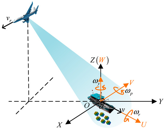
Figure 1.
Geometric diagram of the corner reflector jamming scenario.
2.1. Motion Model of Ship
In Figure 1, the navigation speed of the ship target is , and the heading angle is . The swing motion is described by the body coordinate system , which includes the roll motion around the ship’s long axis , with a rotation angle of ; the pitch motion around the ship’s short axis , with a rotation angle of ; and the yaw motion around the -axis, with a rotation angle of . The three-dimensional swing motion of the ship target is typically represented by the multiplication of three rotation matrices:
where denotes the sinusoidal oscillation angle of rotation around each axis, and , and represent the amplitude, period, and the initial phase of the sinusoidal oscillation, respectively. Suppose that the initial coordinates of the scattering point on the ship are . Then, the instantaneous coordinate of the can be expressed as
where the first term represents the instantaneous coordinates resulting from the ship’s navigation movement, is the projection of the navigation speed onto the -axis, and is the projection of the navigation speed onto the -axis. The second term represents the instantaneous coordinates caused by the swaying motion. Since the swaying motion is described in the body coordinate system , it is necessary to transform it into the coordinate system by multiplying it with a transformation matrix . According to the geometric relationship between the two coordinate systems in Figure 1, the transformation matrix between the two coordinate systems is
2.2. Motion Model of Corner Reflector Array
Due to the small size and light weight of the sea surface inflatable corner reflector, it is assumed that the corner reflectors perform a highly heaving motion with sea surface fluctuation. And the sea surface, as a rough surface, can be modeled by a statistical power spectrum. This paper employs the Elfouhaily power spectrum to establish a two-dimensional dynamic sea surface model, whose expression is as follows:
where represents the wavenumber of the ocean waves, and is the angle between the observation direction and the wave direction. The Elfouhaily spectrum varies with the direction of the sea waves and the wavenumber of the constituent waves, and it is composed of an omnidirectional wavenumber spectrum and a directional function . describes the distribution of the energy across wavenumbers without considering the direction, and it is the sum of the spectrum of two mechanisms:
where and represent the long-wave curvature spectrum and short-wave curvature spectrum, respectively, and their values depend on the wind direction and the wind speed at 10 m from the sea surface. reflects the probability distribution of all constituent waves of the sea wave over angles, and it is a description of the directional characteristics of sea waves. It can be expressed as
where is the upwind–crosswind ratio, which varies with the direction of the wind. The detailed equations of and are shown in Ref. [47].
According to the statistical model of the power spectrum, the Monte Carlo method is utilized to generate random sea surface height [48]. The size of the sea surface grid is , and the length and width are and , respectively. According to the Wiener–Khinchin theorem, it can be deduced that the power spectrum of a signal is the square of the absolute value of its Fourier transform. Therefore, based on the two-dimensional statistical power spectrum model, a statistical model of the two-dimensional wavenumber spectrum of the sea surface can be obtained. By multiplying with random numbers, the calculation formula for the wavenumber spectrum of a random sea surface is as follows:
where and represent the projected wavenumbers of the two-dimensional sea surface grid, denotes a random number with a normal distribution of mean 0 and variance 1. The above formula establishes the random wavenumber spectrum of a two-dimensional sea surface, characterizing sea wave properties in the spatial domain. To generate a dynamic two-dimensional sea surface, it is also necessary to establish a characteristic description of the temporal dimension. According to linear wave theory, there is a certain relationship between wavenumber and frequency, known as the dispersion relation, which is expressed as [48]
where is the gravity acceleration. Using the dispersion relationship, the wavenumber spectrum for a dynamic two-dimensional sea surface can be derived, with the expression
By performing two-dimensional FFT on the above equation, the sea surface height in the spatial domain can be obtained as follows:
The corner reflector array is placed in the sea grid, and the instantaneous coordinate of the scattering point on the corner reflector array is
2.3. Signal Model
Based on the motion model and the instantaneous coordinates of the ship target and corner reflector array, the instantaneous range between the radar and the scattering point can be obtained as follows:
where and represent the instantaneous coordinate of the radar and the scattering point , respectively. Assuming that the radar transmits a linear frequency modulation signal, the echo signal of the marine target after pulse compression is
where is the bandwidth and is the wavelength, and represent the fast time and the slow time, respectively, denotes the time-varying amplitude of the scattering point, and is the number of scattering points of the marine target.
After SAR range migration correction, the range curve caused by radar motion is corrected, leaving the range walk caused by the unknown movement of the target. Then, the azimuth pulse compression function is constructed as follows:
where represents the range corresponding to each range cell. Multiplying the above formula with the signal after migration correction and performing an azimuth FFT, the SAR image data of the scenario can be obtained as follows:
where and represent the residual range and the residual Doppler history caused by the unknown motion, respectively, is the azimuth Doppler, denotes Fourier transform, denotes convolution, and is the observation time of the scenario. Then, target detection is performed to isolate the target slice from the SAR image. Through the application of azimuth FFT and envelope alignment processing, the envelope signal of the detected target is then obtained:
where is the nearest range. The signal of each range cell can be modeled as a multi-component amplitude modulation–frequency modulation (AM-FM) signal.
3. Analysis of the Residual Doppler Characteristics
To achieve unified refocusing processing for marine targets in the corner reflector jamming scenario, it is necessary to analyze the residual Doppler characteristics caused by the unknown motions of the targets and design a suitable and robust processing flow based on the different parameter distribution characteristics. Based on the motion model and signal model previously discussed, this section derives the residual Doppler for ship targets and corner reflector arrays.
3.1. Analysis of the Residual Doppler of a Ship
The instantaneous range between the radar and the scattering point of the ship can be decomposed into the translational range and the rotational range . is the instantaneous range between the radar and the oscillation center of the ship. Assuming that the coordinate of the oscillation center is and the instantaneous coordinate of the radar is , the translational instantaneous range of the ship target is
The first- to third-order derivatives of can be expressed as
It can be seen from the above equation that the values of the third-order derivative and the second term of the second-order derivative are very small and can be ignored. Since the Doppler frequency chirp rate of the azimuth filtering function of SAR imaging is , the residual translational Doppler center and Doppler chirp rate are approximately expressed as
Observing the above equation, we can find that the translation of the ship brings about the Doppler center offset related to and the residual Doppler chirp rate related to .
The rotational range can be approximated as the projection of the rotated coordinate vector onto the line of sight (LOS) and can be expressed as
where is the direction of the LOS, which is approximately equal to the nearest range , represents 2-norm, represents matrix transpose, and represents the instantaneous coordinate of the swing motion of the scattering point. The first- to third-order derivatives of are as follows:
where , , and represent the first- to third-order derivatives, respectively. Then, the calculation equations of swing Doppler center , chirp rate , and quadratic chirp rate are as follows:
It can be seen from the above equation that the Doppler center, chirp rate, and quadratic chirp rate caused by swing motion are linearly related to the three-dimensional coordinates of the scattering points. The value of the correlation coefficient depends on the LOS vector, the attitude angle of the ship, the swing parameter matrix, and their derivatives to time. Consequently, the Doppler parameters of the aggregated scattering points across the ship exhibit close values. To complete the separation and reconstruction of these aggregated scattering points, a high time–frequency resolution is indispensable.
3.2. Analysis of the Residual Doppler of Corner Reflector Array
According to (11), the instantaneous range of the corner reflector is
By performing a Taylor expansion for at , we can obtain the first- to third-order derivatives as follows:
where is the range of the corner reflector at . Then, the residual Doppler parameters of the corner reflector are as follows:
From the above equation, it can be observed that the residual Doppler parameter of the corner reflector depends on the dynamic sea surface height function and its derivative. According to the theory of ocean dynamics, it is recognized that sea surface fluctuations can be regarded as harmonic oscillations, leading to two primary motion states for the corner reflector: it rises and falls with the fluctuations. Furthermore, the continuity of the sea surface allows the motion state to propagate across the sea surface. Therefore, the motion correlation of corner reflectors decreases with an increase in the distance between the corner reflectors and is influenced by the wavelength of the wave, the direction of propagation, and other factors. This results in the Doppler parameter distributions of the corner reflector array appearing random. Additionally, within the same range cell, the Doppler histories of corner reflectors may overlap due to varying motion trends, which will lead to amplitude and phase distortions at the intersection area. These distortions may impact the accuracy of component reconstruction.
In summary, the ship target exhibits a continuous, rigid structure composed of a high density of scattering points, and the Doppler parameters are linearly related to their three-dimensional positions. Conversely, the corner reflector array consists of a non-rigid structure with fewer scattering points and a sparser distribution, and their Doppler parameters are randomly distributed. The distinct physical and motion properties of these two target types within the scene demand that a unified imaging algorithm be designed with enhanced robustness.
4. Proposed Algorithm
This section proposes a unified imaging method of marine targets in the corner reflector jamming scenario based on time–frequency analysis and the modified Clean technique, considering the different Doppler distribution characteristics of ship targets and corner reflector arrays. By using STFT filtering for component extraction, multiple aggregated scattering points on the ship target can be extracted simultaneously, reducing the number of iterations. Applying FrFT and azimuth interpolation, the amplitude and phase of the component with intersecting Doppler frequencies are corrected, minimizing the error in component reconstruction. Figure 2a shows the flowchart of the proposed algorithm, and Figure 2b illustrates the specific steps of the modified Clean technique. The detailed steps of the proposed algorithm are as follows:
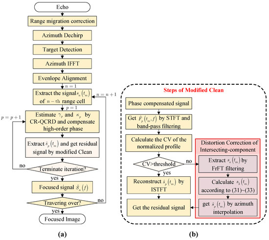
Figure 2.
Flowchart of the proposed method. (a) The overall process of the proposed method. (b) The detailed steps of the modified Clean technique.
Step 1: Perform range migration correction and azimuth dechirp on the pulse compression echo data to obtain the SAR image of the scenario.
Step 2: Perform target detection, azimuthal IFFT, and envelope alignment on the SAR image to obtain the target’s envelope signal.
Step 3: Extract the signal of the range cell of the target.
Step 4: Employ CR-QCRD to estimate the chirp rate and the quadratic chirp rate of the scatter point component, and based on the estimated Doppler parameters, construct a compensation function for high-order phase compensation according to Formulas (26) and (27), obtaining the phase compensated signal .
Step 5: Perform STFT on and apply band-pass filtering according to Formula (31) to obtain the time–frequency distribution of the component . Calculate the coefficient of variation (CV) of the normalized profile image of at and compare it with the threshold; if it is greater than the threshold, then distortion correction is required. FrFT filtering is carried out according to Formulas (34) and (35), and the signal is obtained based on Formulas (37)~(39). Azimuth interpolation is performed on to correct the amplitude and phase distortion, resulting in the component . If it is less than the threshold, then perform an ISTFT according to Equation (32) to obtain the reconstructed signal .
Step 6: Subtract from and multiply the conjugate of to obtain the residual signal.
Step 7: Calculate the kurtosis of the residual signal and compare it with the threshold. If it is less than the threshold, terminate the iteration and output the focused signal of the -th range cell. Otherwise, repeat steps 4 to 6.
Step 8: Determine whether all range cells have been traversed; if so, output the finely focused target image; otherwise, repeat steps 3 to 7.
The following introduces some key steps in the algorithm, including parameter estimation and phase compensation, the modified Clean technique, and iterative termination conditions, and discusses the computational complexity of the algorithm.
4.1. Parameter Estimation and Phase Compensation
The swing motion of the ship and the heaving motion of the corner reflector in the corner reflector jamming scenario bring about complex Doppler modulation with spatial variation. However, in a short period, the echo can be modeled as a CPS, and it can be focused on by designing a phase compensation function based on the estimation of the Doppler chirp rate and the second-order chirp rate. This manuscript applies a Doppler parameter estimation method based on the CR-QCRD proposed in Ref. [45]. By constructing the fourth-order instantaneous autocorrelation function of the signal and applying the GKT and NUFFT, the one-dimensional time domain signal is converted into a two-dimensional domain characterized by the chirp rate and quadratic chirp rate parameters. The location of the maximum peak in this parameter domain corresponds to the chirp rate and the quadratic chirp rate of the component. Compared with other parameter estimation methods for CPS signals, there is no need to preset the range of parameters for parameter search, and the calculation amount is small. In addition, the nonlinear transformation and interpolation operations make it difficult to accumulate the energy of noise and cross terms, which provides better noise immunity and is more suitable for multicomponent signals.
After estimating the chirp rate and quadratic chirp rate of the component, the phase compensation function can be constructed as
By multiplying the signal of the -th range cell with , we can obtain
where is the component to be estimated, and represents other components. After phase compensation, only contains the constant phase and the linear phase, and its Doppler center can be estimated by extracting the position of the peaks with the highest amplitude of . can be expressed as
4.2. Modified Clean Technique
The traditional Clean technique has two ways to eliminate components. The first is to reconstruct the signal by the estimates of the Doppler parameters and amplitude and then directly subtract the reconstructed signal in the time domain. The expression for the reconstructed signal is
where is the number of azimuth sampling points, and is the maximum amplitude of the spectrum of . The above equation does not take into account the constant phase and time-varying amplitude of the component signal. The inequality in the initial phase between the reconstructed component and the actual component indicates that the angles of the two signals in the complex plane do not align and that direct subtraction will generate a new signal. Moreover, because the main lobe width of the time-varying amplitude signal is broader than that of the constant amplitude signal, direct subtraction does not completely eliminate the component, leading to multiple iterations. Taking the first component in Table 1 as an example to simulate the influence of the constant phase and time-varying amplitude on the residual signal, the results are shown in Figure 3. It can be observed that the mismatch of the constant phases leads to the generation of a new signal with an amplitude greater than the original signal, and the time-invariant amplitude of the components results in the residual signal retaining the energy of the estimated component.

Table 1.
Parameters of the simulation components.
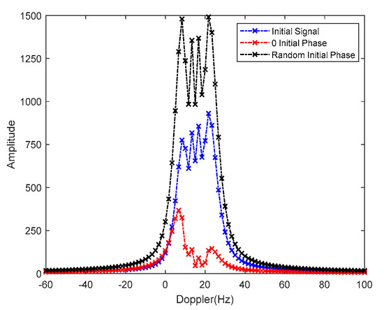
Figure 3.
Influence of initial phase on residual signal.
Another method of the Clean technique involves applying a band-rejection filter to the phase-compensated signal. When the frequency bands of the components intersect, this filter concurrently eliminates energy from the overlapping sections, leading to inaccuracies in amplitude estimation. In order to solve the above problems, this manuscript utilizes STFT filtering to reconstruct the focused component. First, extracting the time–frequency distribution of the focused component by performing a band-pass filter to the time–frequency distribution of the signal , and are expressed as
where is the window function of the STFT, is the frequency band of the band rejection filter. Then, reconstructing the component by applying the inverse short-time Fourier transform (ISTFT) to , the expression is given by
where represents the value of the window function at time 0. The residual signal is obtained by subtracting from , and multiplying the conjugate of , the expression is
In this scenario, the Doppler parameters of the aggregated scattering points across the ship exhibit close values, and after phase compensation, each component is well focused. In cases where the Doppler history differences among the components are smaller than the frequency resolution of the time–frequency image, the associated time–frequency ridges coincide, resulting in their inseparability within the time–frequency plane, as demonstrated in Figure 4a. The simulation signal contains the first and second components in Table 1. Figure 4b shows a comparison of the signal before and after phase compensation. It can be found that both components are focused. In this case, all focused components can be eliminated simultaneously to reduce the number of iterations. Therefore, the bandwidth of the band-pass filter should be adaptive. In this manuscript, the main lobe of the frequency profile at from the time–frequency image is used as the bandwidth for the band-pass filter . Figure 4c shows the normalized one-dimensional frequency profile of and the corresponding band-pass filter function.
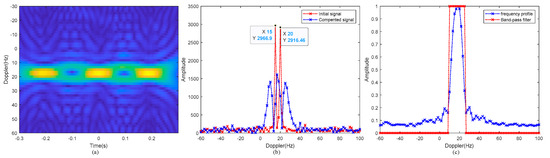
Figure 4.
STFT filtering processing of the signal contains the first and second components. (a) STFT image; (b) the signals before and after phase compensation; (c) the normalized frequency profile of the STFT image and the band-pass filter.
Additionally, the time–frequency ridges of the corner reflector array components may overlap, and the signals in the overlapping portions are influenced by their correlation, resulting in a certain degree of amplitude and phase distortion.
By comparing the CV of the normalized profile of at with a predefined threshold, it is determined whether distortion correction is needed. CV is an indicator to measure the degree of dispersion of variables, which is the ratio of the standard deviation to the mean; a higher value indicates a greater degree of dispersion of the variable. The distortion correction method is introduced with two intersecting components as examples. Firstly, the signal is transformed into the frequency-fraction domain by FrFT, which is defined as
where is the kernel function of FrFT, and it can be expressed as
where , the th-order FrFT of the signal is equivalent to rotating the time–frequency plane by angle . By rotating a certain angle , the LFM signal can be focused on the frequency in the FrFT domain. The relationship between the frequency parameters of the LFM signal and the optimal parameters of the FrFT is
Then, the frequency band of each component can be calculated according to Equation (35). By judging whether contains , it is further determined whether there is a component intersecting with the estimated component. If is not included in , no distortion correction is necessary; otherwise, distortion correction is required. First, the optimal order for the intersecting component is determined, and a frequency domain filter is applied to based on to eliminate the component that does not intersect with the estimated component and obtaining the signal . contains the focused component and the intersecting component , that is,
Then, performing th-order FrFT filtering on to obtain the signal , which contains the intersecting component and the overlapping part of the component , we obtain
Subtracting (36) from (37), we obtain
From the above equation, is equal to minus the intersecting part, has a decrease in amplitude and a sudden change in phase during the overlapping period, and it is necessary to correct the amplitude and phase. Since has been focused on, its phase is linear, phase correction can be performed by linear fitting, and amplitude distortion correction is achieved through interpolation.
Figure 5 and Figure 6 show the simulation results of the distortion correction, where the two-component signals are generated by superimposing component 1 and component 3 from Table 1, as well as component 2 and component 3, with the signal–noise ratio (SNR) set to 0 dB. The STFT images of the two-component signals are shown in Figure 5a and Figure 6a, from which it can be observed that the energy is enhanced at the intersection of component 1 and component 3, while the energy is weakened at the intersection of component 2 and component 3. This is because the phase difference between the signals at the intersection is different, leading to different results after vector addition. The results after band-pass filtering are shown in Figure 5b and Figure 6b. It can be seen that the amplitude of the time–frequency ridge of has a certain oscillation and obvious distortion. The phase fitting error and amplitude history of are shown in Figure 5c and Figure 6c, where the red box represents the intersection part, which has an obvious phase fitting error and amplitude decrease. The STFT image of the signal after interpolation correction and band-pass filtering is shown in Figure 5d and Figure 6d. It can be seen that the amplitude of the time–frequency ridge of s changes gently. The comparison results of residual signals before and after distortion correction are shown in Figure 5e and Figure 6e. It can be seen that the spectral amplitude of the residual signal without distortion correction decreases abruptly, which affects the amplitude estimation accuracy of the subsequent intersecting component. In contrast, the spectrum of the distortion-corrected residual signal is close to the ideal residual component.
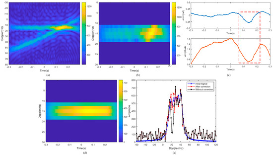
Figure 5.
Distortion correction processing of the signal contains the first and the third component. (a) STFT image; (b) STFT image after band-pass filtering; (c) amplitude and phase distortion of ; (d) STFT image after distortion correction; (e) comparison of residual signals before and after distortion correction.
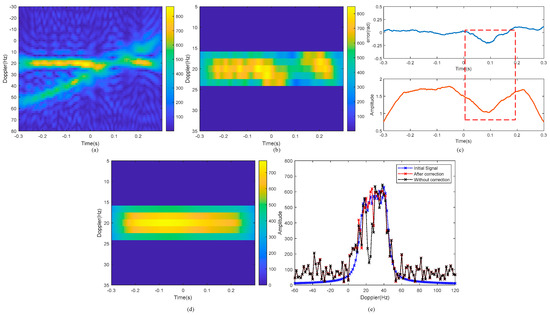
Figure 6.
Distortion correction processing of the signal contains the second and the third component. (a) STFT image; (b) STFT image after band-pass filtering; (c) amplitude and phase distortion of ; (d) STFT image after distortion correction; (e) comparison of residual signals before and after distortion correction.
4.3. Iteration Termination Condition
The traditional Clean technique takes the energy attenuation ratio as the iteration termination condition, which makes it difficult to set the appropriate threshold, and it is easy to generate false scattering points at low SNR. This manuscript expects to add an iterative termination condition through signal feature analysis to reduce the number of iterations and avoid the generation of false scattering points. When there are components in the residual signal, the energy of the signal spectrum is concentrated in the frequency bands of the components, resulting in a high degree of concentration of the spectrum amplitude. In contrast, when the residual signal contains only noise and sea clutter, the energy of the signal spectrum is dispersed across the entire frequency band, leading to a low degree of concentration of the spectrum amplitude. The concentration of the spectrum amplitude can be measured by kurtosis, which is an indicator describing the dispersion degree of random variables. The calculation equation for the kurtosis of variable is
where and are the mean and the standard deviation of the variable, respectively, and represents the mathematic expectation. The larger the , the greater the degree of dispersion of variable distribution. The kurtosis value for a normally distributed random variable is 3. Based on extensive experience in processing large amounts of data, the threshold for kurtosis can be set to 4.
4.4. Computational Complexity
Since the processing speed is very important in practical applications of the algorithm, this section analyzes the computational complexity of the proposed algorithm. Taking a multi-component signal in a range cell as an example, assume that the length of the signal is . Firstly, the computational complexity of the phase compensation step is analyzed. In phase compensation, the key step is the CR-QCRD parameter estimation, which includes GKT and NUFFT. The interpolation operation of GKT can be rapidly calculated using the scaling Fourier transform–inverse fast Fourier transform, with a computational complexity of . NUFFT achieves rapid computation through interpolation and FFT, and its computational complexity is . Next, the computational complexity of the Clean step is analyzed. Depending on the different characteristics of the Doppler distribution, two different Clean methods are distinguished. The steps with higher computational complexity in the two methods are STFT filtering and FrFT filtering, respectively. The computational complexity of STFT is related to the window length and is . FrFT can be rapidly calculated using the Chirp-Z transform, with a computational complexity of . Therefore, the computational cost of the proposed algorithm is .
5. Simulation
In this section, according to the simulated data, the proposed method is compared with the FrFT-WVD algorithm [35] and the CR-QCRD algorithm [45]. Firstly, the reconstruction accuracy and iteration number of multi-component signals are simulated and compared under different SNRs. Then, the simulation compares the focusing results of the marine targets in the corner reflector jamming scenarios. The residual signal energy attenuation ratio threshold for the iteration termination condition of the FrFT-WVD algorithm and the CR-QCRD algorithm is set to 0.1, and the maximum number of iterations is set to 20.
5.1. Simulation for the Multicomponent AM-CPS Signal
In this section, the reconstruction accuracy and iterative number of the three algorithms are simulated under different SNRs. Two multi-component AM-CPS signals are generated according to the motion model of the ship and the corner reflector array, respectively. The RCS and the Doppler parameters of each component are shown in Table 2 and Table 3. The first signal contains five components, three of which are aggregated scattering points with similar Doppler parameters; the second signal contains three components, two of which intersect with each other, and the Doppler curves for each component of the two signals are shown in Figure 7.
Table 2.
Parameters of the first signal.
Table 3.
Parameters of the second signal.
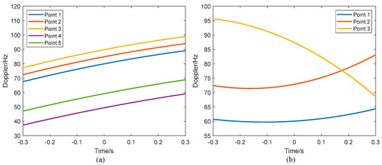
Figure 7.
Doppler history of the components of the two signals. (a) The first signal; (b) the second signal.
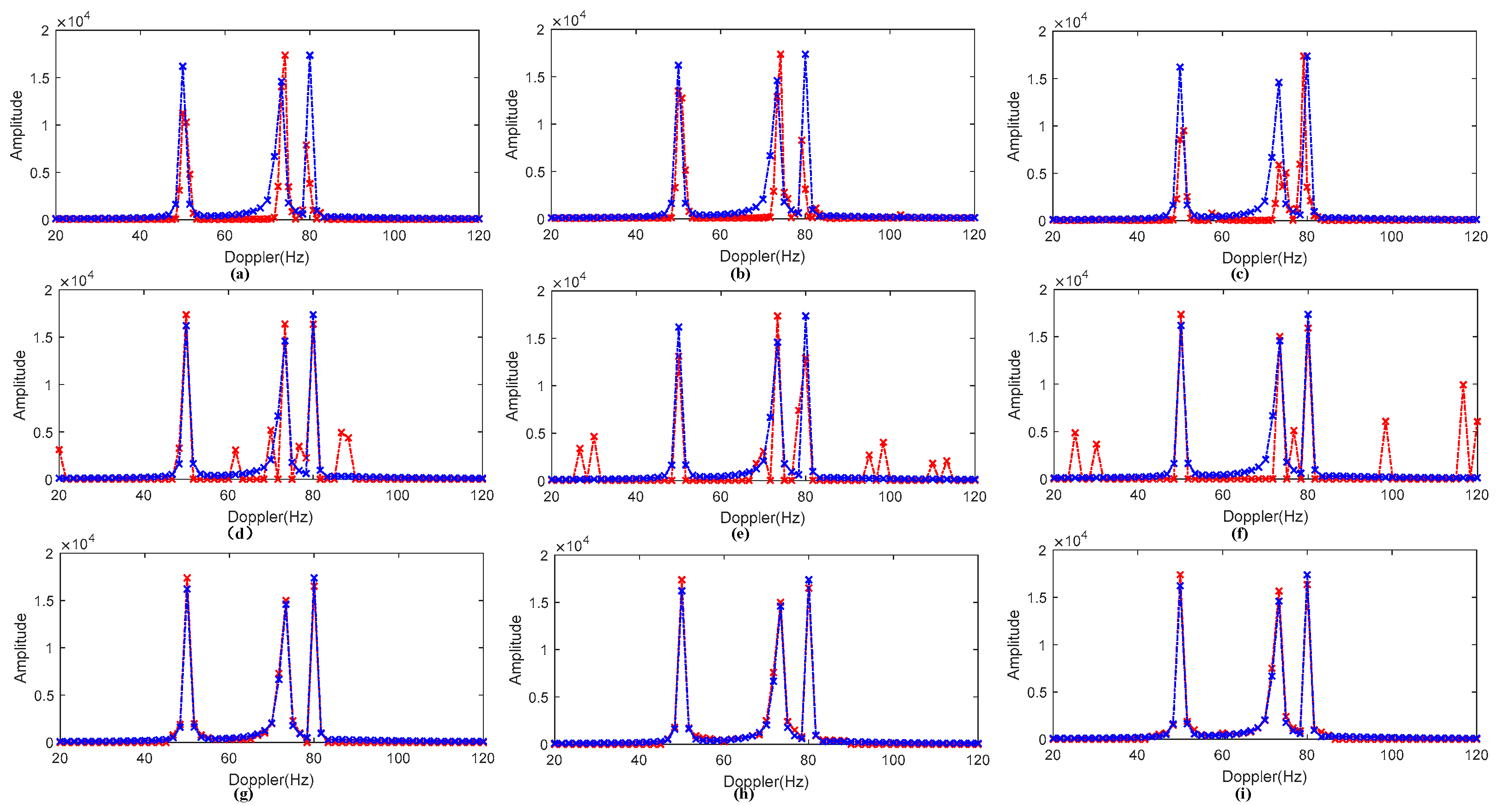
The focusing results of the three methods for the two signals under different SNRs are shown in Figure 8 and Figure 9. Figure 8a–c and Figure 9a–c show the focusing result obtained by the FrFT-WVD algorithm. It can be seen from Figure 8a–c that the reconstruction accuracy of the FrFT-WVD algorithm decreases with decreasing SNR and that the three aggregated scattering point components are not separated at −5 dB SNR. From Figure 9a–c, it can be noticed that the error of the estimation results is relatively large, because the FrFT-WVD algorithm removes the components by windowing in the frequency domain, which also removes part of the intersecting components. Figure 8d–f and Figure 9d–f show the focusing results obtained by the CR-QCRD algorithm, from which we can find that there are many false points. Figure 8h–i and Figure 9h–i show that the proposed method can realize the accurate reconstruction of each component in the signal under different SNR conditions.
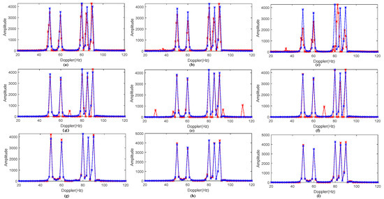
Figure 8.
Comparison of the focusing results of the first signal. (a–c): The focusing results obtained by FrFT-WVD under different SNR conditions: (a) SNR = 5 dB, (b) SNR = 0 dB, and (c) SNR = −5 dB. (d–f): The focusing results obtained by CR-QCRD under different SNR conditions: (d) SNR = 5 dB, (e) SNR = 0 dB, and (f) SNR = −5 dB. (g–i): The focusing results obtained by the proposed method under different SNR conditions: (g) SNR = 5 dB, (h) SNR = 0 dB, and (i) SNR = −5 dB.
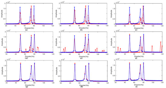
Figure 9.
Comparison of the focusing results of the second signal. (a–c): The focusing results obtained by FrFT-WVD under different SNR conditions: (a) SNR = 5 dB, (b) SNR = 0 dB, and (c) SNR = −5 dB. (d–f): The focusing results obtained by CR-QCRD under different SNR conditions: (d) SNR = 5 dB, (e) SNR = 0 dB, and (f) SNR = −5 dB. (g–i): The focusing results obtained by the proposed method under different SNR conditions: (g) SNR = 5 dB, (h) SNR = 0 dB, and (i) SNR = −5 dB.
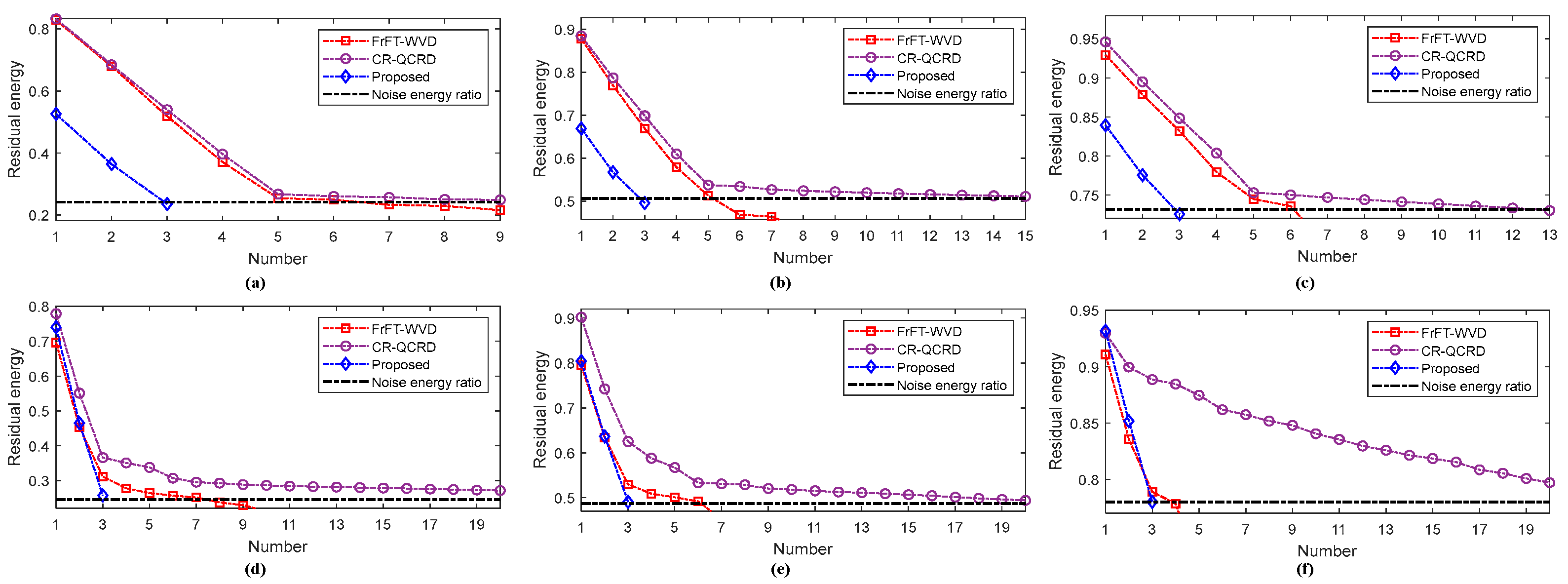
The residual energy iteration curves of the three algorithms under different SNRs are shown in Figure 10, from which it can be found that the residual energy ratios of the FrFT-WVD and CR-QCRD algorithms tend to different values under different SNRs. Therefore, the iteration termination condition based on the residual energy ratio has poor adaptability. By comparison, the iteration termination condition using kurtosis can reliably end the iteration process across various SNR levels, demonstrating robust stability. Furthermore, as observed in Figure 10a–c, the residual energy ratio after the first iteration of the proposed method is nearly equivalent to that of the third iteration of the other two methods. This is because the three aggregated scattering points are simultaneously removed by STFT filtering at one time, and the proposed method requires only three iterations. Therefore, the proposed algorithm can save computational resources by reducing the number of iterations when processing ship targets.
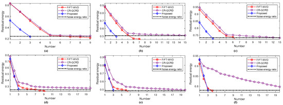
Figure 10.
Comparison of the iterative number of the three algorithms under different SNRs. (a–c): The iterative number of the first signal: (a) SNR = 5 dB, (b) SNR = 0 dB, and (c) SNR = −5 dB. (d–f): The iterative number of the second signal: (d) SNR = 5 dB, (e) SNR = 0 dB, and (f) SNR = −5 dB.
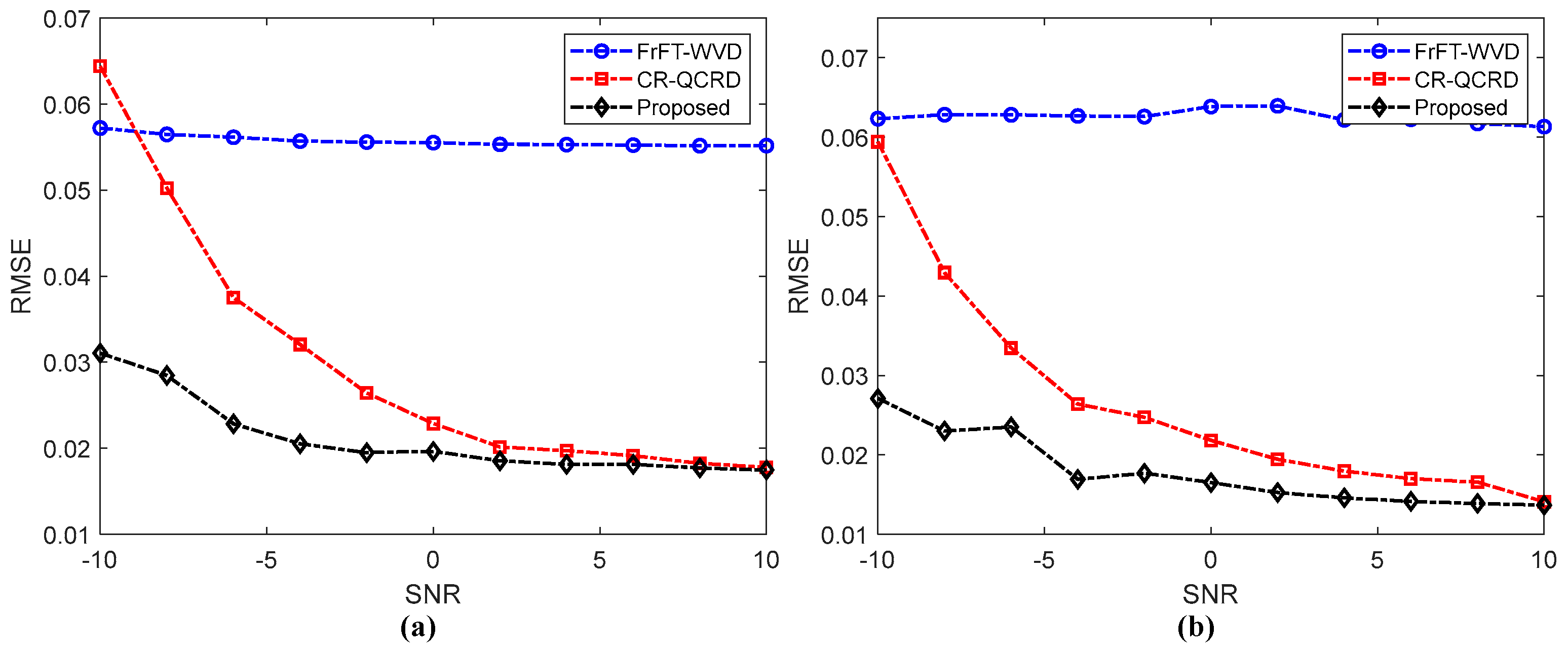
To further verify the reconstruction accuracy of the proposed algorithm, 100 Monte Carlo experiments are designed under the condition of −10~10 dB SNR. The root mean square error (RMSE) is used as the evaluation index. The definition equation of RMSE is
The smaller the value of RMSE, the higher the reconstruction accuracy. Figure 11 shows the average RMSE values across the various SNR conditions. It is evident that the FrFT-WVD algorithm has a higher RMSE, indicating lower reconstruction accuracy. As the SNR decreases, the RMSE of both the CR-QCRD algorithm and the proposed algorithm drops. The RMSE of the CR-QCRD algorithm decreases rapidly, and its average RMSE is nearly equal to that of the FrFT-WVD algorithm at −10 dB. In contrast, the RMSE of the proposed method decreases more gradually, and it maintains the lowest RMSE under all SNR conditions. In summary, the proposed algorithm can reconstruct signals more accurately.
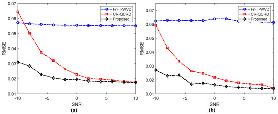
Figure 11.
Average RMSE of the three algorithms under different SNRs: (a) first signal; (b) second signal.
5.2. Simulation for Marine Targets in the Scenario
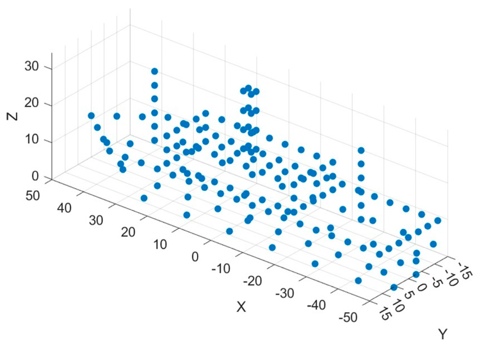
In this section, the simulation verifies the imaging results of the ship and the corner reflector array in the jamming scenarios under different sea states. The parameters of the radar system are shown in Table 4, and according to Ref. [18] as well as the Beaufort scale, the swing parameters of the ship target and the wind speed parameters of the wave power spectrum under the sea conditions of level 3 and level 5 are shown in Table 5. The ship target sails at a speed of 7 m/s. A three-dimensional model of the ship target is shown in Figure 12, containing 177 scattering points and measuring 100 m in length, 25 m in width, and 30 m in height. The corner reflector array contains 22 scattering points, forming a rectangular array; the length and width of the rectangle are consistent with that of the ship target. Gaussian white noise is added to the echoes to generate data with −5 dB SNR.
Table 4.
Parameters of the radar system used in the simulation.
Table 5.
Parameters of swing motion used in the simulation.
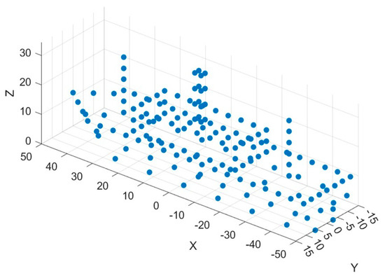
Figure 12.
Model of the ship.
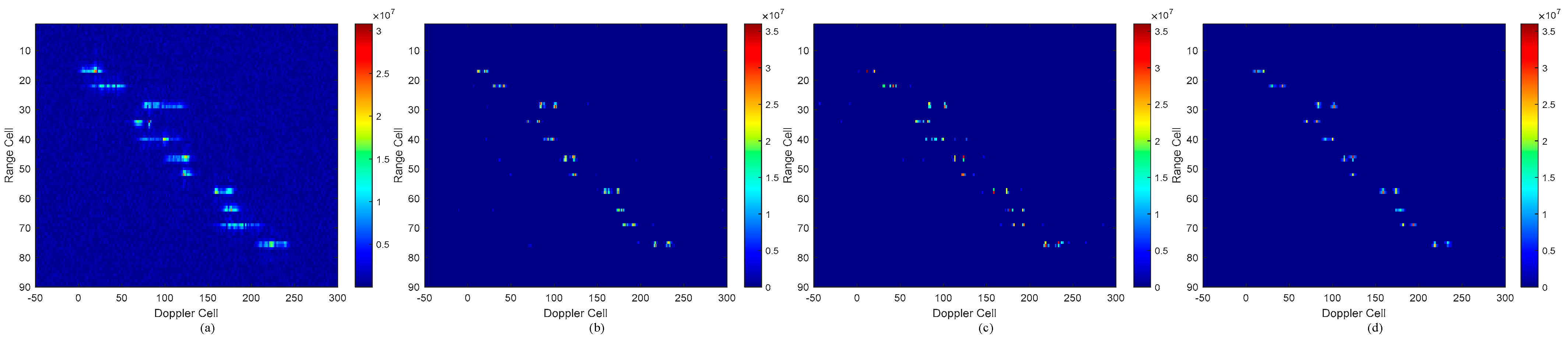
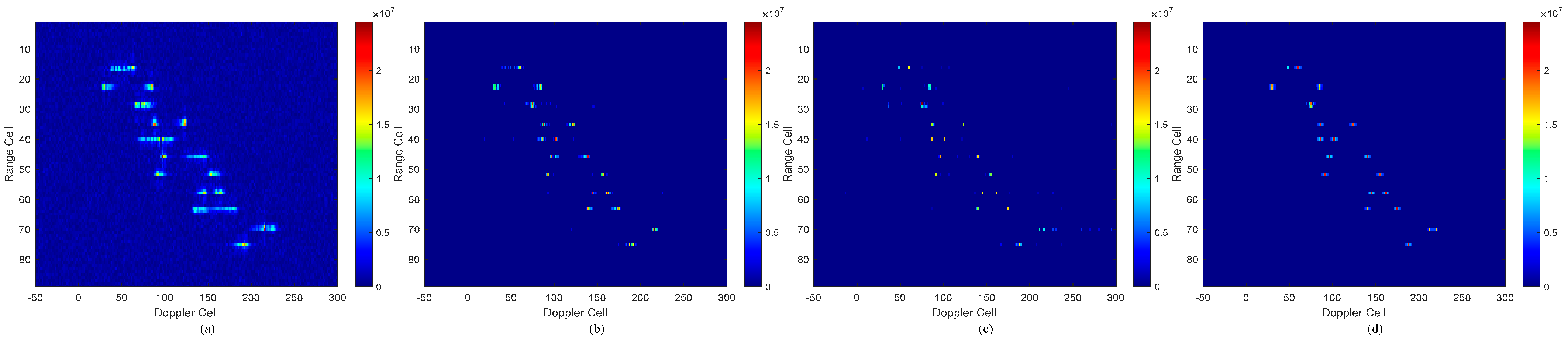
The focusing results of the three algorithms on the ship and the corner reflector array are shown in Figure 13, Figure 14, Figure 15 and Figure 16. Figure 13a, Figure 14a, Figure 15a and Figure 16a show the SAR images of the marine target; it can be noticed that the spatially varying Doppler parameters lead to an inconsistent degree of defocusing of the scattering points on the target. Figure 13b and Figure 14b show the focusing results of the FrFT-WVD algorithm on the ship, from which the outline of the ship can be seen clearly, but there are main lobe broadening of the scattering points and slight false point interference. Figure 15b and Figure 16b show the focusing results of the FrFT-WVD algorithm for the corner reflector array. It can be seen that some scattering points are defocused. Figure 13c, Figure 14c, Figure 15c and Figure 16c show the focusing results of CR-QCRD. There are many false points in the image, and the contour of the ship target in Figure 13c is not clear. The proposed algorithm has a good focusing effect for both the ship and the corner reflector array, with clear ship contours, good focusing of corner reflectors, and no false point interference. Therefore, the proposed algorithm is more suitable for practical applications than other algorithms.
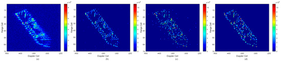
Figure 13.
Imaging results of ship target under sea state 3. (a) SAR; (b) FrFT-WVD; (c) CR-QCRD; (d) proposed method.
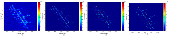
Figure 14.
Imaging results of ship target under sea state 5. (a) SAR; (b) FrFT-WVD; (c) CR-QCRD; (d) proposed method.
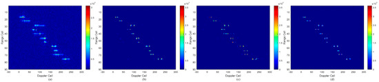
Figure 15.
Imaging results of corner reflector array under sea state 3. (a) SAR; (b) FrFT-WVD; (c) CR-QCRD; (d) proposed method.
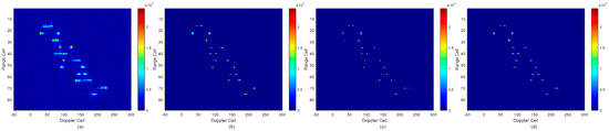
Figure 16.
Imaging results of corner reflector array under sea state 5. (a) SAR; (b) FrFT-WVD; (c) CR-QCRD; (d) proposed method.
In the above process of imaging, the Doppler parameters of the scattering points in the target are also extracted, and these data can be further analyzed to mine some distinguishable features of marine targets, such as the clustering feature and the average correlation coefficient. Through clustering analysis of the Doppler parameters, the maximum cluster size is extracted as a global feature to evaluate the connectivity of the parameter distribution. Additionally, the average Pearson correlation coefficient between Doppler histories in the neighboring range cells is computed as a local feature to gauge the inter-parameter correlations. The results are shown in Table 6 and Table 7. Clearly, there is a significant difference in the maximum cluster size of the Doppler parameters between the two types of targets.
Table 6.
Features of Doppler parameters of marine targets under sea state 3.
Table 7.
Features of Doppler parameters of marine targets under sea state 5.
6. Conclusions
This manuscript proposed an imaging method of marine targets in the corner reflector jamming scenario based on time–frequency analysis and the modified Clean technique. First, the motions of the ship and the corner reflector array were modeled, and the Doppler parameter distribution characteristics of the two types of targets were analyzed. The Doppler parameters of the ship are linearly correlated with the three-dimensional coordinates of the scattering points, while the Doppler parameters of the corner reflector array are approximately random. Then, the Clean technique was adapted to accommodate the different Doppler distribution characteristics. On the one hand, STFT filtering was applied to reconstruct and extract components, thereby reducing the iteration count. On the other hand, FrFT filtering combined with interpolation was used to correct the amplitude–phase distortions of the overlapping Doppler history of corner reflectors, minimizing reconstruction errors. In addition, we utilized kurtosis as the criterion for terminating iterations, which has better anti-noise performance and stability. The simulation results show that the proposed method is more effective and suitable for corner reflector jamming scenarios.
The proposed algorithm can be applied to sea observation by airborne or spaceborne SAR platforms with medium resolution and a short synthetic aperture time. Since the proposed algorithm assumes that the echo signal follows a cubic phase model, this model is no longer applicable under high resolution and a long synthetic aperture. Subsequent research can continue to explore parameter estimation algorithms that do not rely on the echo signal model.
The Doppler parameters obtained by the proposed algorithm during the imaging process contain distinguishable identification features that can offer critical information for target identification. Therefore, further investigation and analysis are essential in future studies.
Author Contributions
C.C. created the research idea, wrote the manuscript, conducted the theoretical analyses, and verified the proposed method; W.L. and Y.G. were involved in improving the proposed method; L.C. and Q.C. designed the experiments; J.F. and M.X. contributed to revising the manuscript. All authors have read and agreed to the published version of the manuscript.
Funding
This research was funded in part by The National Key R&D Program of China under Grant 2022YFB3901604, in part by The Young Scientist Fund of the National Natural Science Foundation of China under Grant 62301389, in part by the Open Fund of the Laboratory of Pinghu.
Data Availability Statement
No new data were created or analyzed in this study. Data sharing is not applicable to this article.
Conflicts of Interest
The authors declare no conflict of interest.
References
- Cerutti-Maori, D.; Klare, J.; Brenner, A.R.; Ende, J.H.G. Wide-area traffic monitoring with the SAR/GMTI system PAMIR. IEEE Trans. Geosci. Remote Sens. 2008, 46, 3019–3030. [Google Scholar] [CrossRef]
- Renga, A.; Graziano, M.D.; Moccia, A. Segmentation of marine SAR images by sublook analysis and application to sea traffic monitoring. IEEE Trans. Geosci. Remote Sens. 2019, 57, 1463–1477. [Google Scholar] [CrossRef]
- Gao, G.; Wang, X.; Lai, T. Detection of moving ships based on a combination of magnitude and phase in along-track interferometric SAR—Part II: Statistical modeling and CFAR detection. IEEE Trans. Geosci. Remote Sens. 2015, 53, 3582–3599. [Google Scholar] [CrossRef]
- Curlander, J.C.; McDonough, R.N. Synthetic Aperture Radar: Systems and Signal Processing, 1st ed.; Wiley-Interscience: New York, NY, USA, 1991. [Google Scholar]
- Moreira, A.; Prats-Iraola, P. A tutorial on synthetic aperture radar. IEEE Trans. Geosci. Remote Sens. Mag. 2013, 1, 6–43. [Google Scholar] [CrossRef]
- Cumming, I.G.; Wong, F.H. Digital Processing of Synthetic Aperture Radar Data; Artech House: London, UK, 2005; Volume 1, pp. 108–110. [Google Scholar]
- Liu, W.; Li, H.; Zhang, J.; Sun, G.C.; Bian, H.; Xiang, J.; Xing, M. On the Role of Scene Coordinate System in Focusing of GEO SAR Data with Fast Time-Domain Algorithm. IEEE J. Sel. Top. Appl. Earth Obs. Remote Sens 2024, 18, 2355–2369. [Google Scholar] [CrossRef]
- Ferrer, P.J.; López-Martínez, C.; Aguasca, A.; Pipia, L.; González-Arbesú, J.M.; Fabregas, X.; Romeu, J. Transpolarizing trihedral corner reflector characterization using a GB-SAR system. IEEE Geosci. Remote Sens. Lett. 2011, 8, 774–778. [Google Scholar] [CrossRef]
- Hu, H.; Zhang, L.; Zhang, X. A study on equipment developments and operational using of ship born gas-filled anti-missile multi-cornerreflector. Def. Technol. Rev. 2018, 39, 74–77. [Google Scholar]
- Luo, Y.; Guo, L.; Zuo, Y.; Liu, W. Time-domain scattering characteristics and jamming effectiveness in corner reflectors. IEEE Access. 2020, 9, 15696–15707. [Google Scholar] [CrossRef]
- Zhang, Z.; Zhao, Y. Analysis of electromagnetic scattering characteristic for new type icosahedrons triangular trihedral corner reflectors. Command Control Simul. 2018, 40, 133–137. [Google Scholar]
- Li, H.; Chen, S.; Wang, X. Study on characterization of sea corner reflectors in polarimetric rotation domain. Syst. Eng. Electron. 2022, 44, 2065–2073. [Google Scholar]
- Li, H.; Chen, S. Electromagnetic scattering characteristics and radar identification of sea corner reflectors: Advances and prospects. J. Radars 2023, 12, 738–761. [Google Scholar]
- Li, H.; Cui, X.; Li, M.; Chen, S. Characterization of corner reflector array in joint space-time-polarization domain. IET Int. Radar Conf. 2023, 2023, 1328–1332. [Google Scholar] [CrossRef]
- Xie, Y.; Xing, M.; Gao, Y.; Wu, Z.; Sun, G.; Guo, L. Attributed Scattering Center Extraction Method for Microwave Photonic Signals Using DSM-PMM-Regularized Optimization. IEEE Trans. Geosci. Remote Sens. 2022, 60, 1–16. [Google Scholar] [CrossRef]
- Zhang, J.; Xing, M.; Xie, Y. A Feature Fusion Framework for SAR Target Recognition Based on Electromagnetic Scattering Features and Deep CNN Features. IEEE Trans. Geosci. Remote Sens. 2021, 59, 2174–2187. [Google Scholar] [CrossRef]
- Duan, D.; Shen, Y.; Wu, Z.; Ou, J. Identification of sea corner reflector array based on spatial morphological features. Fourth Int. Conf. Signal Process. Comput. Sci. 2023, 12970, 382–390. [Google Scholar]
- He, Y.; Yang, H.; He, H.; Yin, J.; Yang, J. A ship discrimination method based on high-frequency electromagnetic theory. Remote Sens. 2022, 14, 3893. [Google Scholar] [CrossRef]
- Doerry, A.W. Ship Dynamics for Maritime ISAR Imaging; Sandia National Laboratories (SNL): Albuquerque, NM, USA; Livermore, CA, USA, 2008. [Google Scholar]
- Schwarz, U.J. Mathematical-statistical description of the iterative beam removing technique (method CLEAN). Astron. Astrophys. 1978, 65, 345. [Google Scholar]
- Tsao, J.; Steinberg, B.D. Reduction of sidelobe and speckle artifacts in microwave imaging: The CLEAN technique. IEEE Trans. Antennas Propag. 1988, 36, 543–556. [Google Scholar] [CrossRef]
- Martorella, M.; Acito, N.; Berizzi, F. Statistical Clean technique for ISAR imaging. IEEE Trans. Geosci. Remote Sens. 2007, 45, 3552–3560. [Google Scholar] [CrossRef]
- Li, X.; Kong, L.; Cui, G.; Yi, W. CLEAN-based coherent integration method for high-speed multi-targets detection. IET Radar Sonar Navig. 2016, 10, 1671–1682. [Google Scholar] [CrossRef]
- Chen, V.C.; Qian, S. Joint time-frequency transform for radar range-Doppler imaging. IEEE Trans. Aerosp. Electron. Syst. 1998, 34, 486–499. [Google Scholar] [CrossRef]
- Berizzi, F.; Mese, E.D.; Diani, M.; Martorella, M. High-resolution ISAR imaging of maneuvering targets by means of the range instantaneous Doppler technique: Modeling and performance analysis. IEEE Trans. Image Process. 2001, 10, 1880–1890. [Google Scholar] [CrossRef] [PubMed]
- Xia, X.G.; Wang, G.; Chen, V.C. Quantitative SNR analysis for ISAR imaging using joint time-frequency analysis-Short time Fourier transform. IEEE Trans. Aerosp. Electron. Syst. 2002, 38, 649–659. [Google Scholar] [CrossRef]
- Auger, F.; Flandrin, P. Improving the readability of time-frequency and time-scale representations by the reassignment method. IEEE Trans. Signal Process. 1995, 43, 1068–1089. [Google Scholar] [CrossRef]
- Hopgood, J.R.; Rayner, P.J.W. Single channel nonstationary stochastic signal separation using linear time-varying filters. IEEE Trans. Signal Process. 2003, 51, 1739–1752. [Google Scholar] [CrossRef]
- Brevdo, E.; Fučkar, N.S.; Thakur, G. The Synchrosqueezing algorithm: A robust analysis tool for signals with time-varying spectrum. Signal Process. 2011, 93, 1079–1094. [Google Scholar]
- Wang, X.; Dai, Y.; Song, S.; Jin, T.; Huang, X. Deep Learning-Based Enhanced ISAR-RID Imaging Method. Remote Sens. 2023, 15, 5166. [Google Scholar] [CrossRef]
- Xing, M.; Wu, R.; Li, Y.; Bao, Z. New ISAR imaging algorithm based on modified Wigner-Ville distribution. IET Radar Sonar Navig. 2008, 3, 70–80. [Google Scholar] [CrossRef]
- Huang, P.; Liao, G.; Yang, Z.; Xia, X.; Ma, J.; Zhang, X. A Fast SAR Imaging Method for Ground Moving Target Using a Second-Order WVD Transform. IEEE Trans. Geosci. Remote Sens. 2016, 54, 1940–1956. [Google Scholar] [CrossRef]
- Bai, X.; Tao, R.; Wang, Z.; Wang, Y. ISAR imaging of a ship target based on parameter estimation of multicomponent quadratic frequency-modulated signals. IEEE Trans. Geosci. Remote Sens. 2013, 52, 1418–1429. [Google Scholar] [CrossRef]
- Li, Y.; Liu, K.; Tao, R.; Bai, X. Adaptive viterbi-based range-instantaneous Doppler algorithm for ISAR imaging of ship target at sea. IEEE J. Ocean. Eng. 2014, 40, 417–425. [Google Scholar] [CrossRef]
- Wang, Y.; Huang, X.; Zhang, Q. Rotation parameters estimation and cross-range scaling research for range instantaneous Doppler ISAR images. IEEE Sens. J. 2020, 20, 7010–7020. [Google Scholar] [CrossRef]
- Li, Z.; Zhang, X.; Qing, Y.; Xiao, Y.; An, H. Hybrid SAR-ISAR Image Formation via Joint FrFT-WVD Processing for BFSAR Ship Target High-Resolution Imaging. IEEE Trans. Geosci. Remote Sens. 2022, 60, 1–13. [Google Scholar] [CrossRef]
- Lv, X.; Xing, M.; Wan, C.; Zhang, S. ISAR imaging of maneuvering targets based on the range centroid Doppler technique. IEEE Trans. Image Process. 2010, 19, 141–153. [Google Scholar]
- Lv, X.; Bi, G.; Wan, C.; Xing, M. Lv’s distribution: Principle, implementation, properties, performance. IEEE Trans. Signal Process. 2011, 59, 3576–3591. [Google Scholar] [CrossRef]
- Ding, Z.; Zhang, T.; Li, Y.; Li, G.; Dong, X.; Zeng, T.; Meng, K. A Ship ISAR Imaging Algorithm Based on Generalized Radon-Fourier Transform With Low SNR. IEEE Trans. Geosci. Remote Sens. 2019, 57, 6385–6396. [Google Scholar] [CrossRef]
- Wang, J.; Leng, X.; Sun, Z.; Zhang, X.; Ji, K. Fast and accurate refocusing for moving ships in SAR imagery based on FrFT. Remote Sens. 2023, 15, 3656. [Google Scholar] [CrossRef]
- O’Shea, P. Improving polynomial phase parameter estimation by using nonuniformly spaced signal sample method. IEEE Trans. Signal Process. 2012, 60, 3405–3414. [Google Scholar] [CrossRef]
- Wu, L.; Wei, X.; Yang, D.; Wang, H.; Li, X. ISAR imaging of targets with complex motion based on discrete chirp Fourier transform for cubic chirps. IEEE Trans. Geosci. Remote Sens. 2012, 50, 4201–4212. [Google Scholar] [CrossRef]
- Zheng, J.; Su, T.; Zhu, W.; Zhang, L.; Liu, Z.; Liu, Q. ISAR imaging of nonuniformly rotating target based on a fast parameter estimation algorithm of cubic phase signal. IEEE Trans. Geosci. Remote Sens. 2015, 53, 4727–4740. [Google Scholar] [CrossRef]
- Huang, P.; Xia, X.; Zhan, M.; Liu, X.; Liao, G.; Jiang, X. ISAR imaging of a maneuvering target based on parameter estimation of multicomponent cubic phase signals. IEEE Trans. Geosci. Remote Sens. 2021, 60, 1–18. [Google Scholar] [CrossRef]
- Yang, S.; Li, S.; Fan, H.; Liu, Y. High-resolution ISAR imaging of maneuvering targets based on azimuth adaptive partitioning and compensation function estimation. IEEE Trans. Geosci. Remote Sens. 2023, 61, 1–15. [Google Scholar] [CrossRef]
- Zheng, J.; Su, T.; Zhang, L.; Zhu, W.; Liu, Q. ISAR Imaging of Targets With Complex Motion Based on the Chirp Rate-Quadratic Chirp Rate Distribution. IEEE Trans. Geosci. Remote Sens. 2014, 52, 7276–7289. [Google Scholar] [CrossRef]
- Elfouhaily, T.; Chapron, B.; Katsaros, K. A unified directional spectrum for long and short wind-driven waves. J. Geophys. Res. Ocean. 1997, 102, 15781–15796. [Google Scholar] [CrossRef]
- Plant, W.J. The Ocean Wave Height Variance Spectrum: Wavenumber Peak versus Frequency Peak. J. Phys. Oceanogr. 2009, 39, 2382–2383. [Google Scholar] [CrossRef]


Disclaimer/Publisher’s Note: The statements, opinions and data contained in all publications are solely those of the individual author(s) and contributor(s) and not of MDPI and/or the editor(s). MDPI and/or the editor(s) disclaim responsibility for any injury to people or property resulting from any ideas, methods, instructions or products referred to in the content. |
© 2025 by the authors. Licensee MDPI, Basel, Switzerland. This article is an open access article distributed under the terms and conditions of the Creative Commons Attribution (CC BY) license (https://creativecommons.org/licenses/by/4.0/).