Infrared Dim Small Target Detection Algorithm with Large-Size Receptive Fields

Abstract

Infrared target detection has a wide range of application value, but due to the characteristics of infrared images, infrared targets are easily submerged in the complex background. Therefore, in complex scenes, it is difficult to effectively and accurately detect infrared dim small targets. For this reason, we design an infrared dim small target (IDST) detection algorithm containing Large-size Receptive Fields (LRFNet). It uses the Residual network with an Inverted Pyramid Structure (RIPS), which consists of convolutional layers that become progressively smaller, so it can have a larger effective receptive field and can improve the robustness of the model. In addition, through the Attention Mechanisms with Large Receptive Fields and Inverse Bottlenecks (LRIB), it can make the network better localize the region where the target is located and improve the detection effect of the model. The experimental results show that our proposed algorithm outperforms other state-of-the-art algorithms in all evaluation metrics.

1. Introduction

Infrared target detection technology has shown strong potential for application in a number of areas due to its characteristics of being unaffected by weather conditions and electromagnetic interference. For timely detection of targets, the detector needs to cover a large area, and is typically located at a great distance from the target, resulting in the target appearing as small and dim points in the image. These types of targets are referred to as infrared dim small targets (IDSTs) [1].

Compared to visible light, infrared images lack texture information, and the boundaries between targets and backgrounds are not very prominent. As a result, it is hard to recognize IDSTs in a complex environment, leading to a decrease in detection rate. Additionally, the phenomenon of blind elements and noise points in the infrared detector can lead to an elevation of the false alarm (FA) rate. Hence, an IDST detection algorithm with high probability of detection (PD) and low FA rate is urgently needed in practical applications [2].

Due to the small size of infrared targets, infrared targets can easily be lost by using a detection network designed for visible targets. Furthermore, the bounding box makes it difficult to accurately determine the location of the target because most IDSTs appear as dots in the image. Therefore, most algorithms for IDST detection are based on image segmentation. Current IDST detection algorithms can generally be divided into two categories: traditional algorithms and deep learning-based algorithms [3].

Traditional target detection algorithms are based on certain previous knowledge and can be broadly categorized as filter-based, human visual system-based, and data structure-based.

Filter-based algorithms remove background information and detect targets by designing specific filters. They have relatively low computational complexity and are easy to implement on various platforms. However, such algorithms are susceptible to noise and clutter, so they can only be applied to simple background scenes [4].

Methods based on the human visual system use contrast to distinguish between targets and the background, which enhances the target and suppresses the background, but they are highly sensitive to object edges and are only suitable for scenes with large differences between the target and background features [5].

Data structure-based algorithms mainly utilize the sparsity of the target and the low-rank nature of the background, transforming target detection into a mathematical problem to be solved. They have good effectiveness and are suitable for most scenes, but the large amount of matrix calculations can make implementation difficult and time-consuming [6].

In recent years, with the advancement of deep learning technology, more and more deep learning algorithms are used in the field of IDST detection. Some algorithms used generative adversarial networks, employing different generators and discriminators to balance the false alarm and missed detection issues in IDST detection [7]. Some algorithms used recurrent skip connections to preserve the detailed information of IDSTs in feature maps for better detection [8].

However, there are still some issues with the existing IDST detection algorithms. Traditional algorithms mostly rely on certain prior knowledge, and their performance is greatly affected when the actual scene does not align with the prior knowledge. Furthermore, while deep learning-based algorithms have made significant improvements over traditional algorithms, they still have some limitations [9].

A new IDST detection algorithm based on CNN is proposed in this paper: Infrared dim small Target Detection Algorithm with Large-size Receptive Fields. It uses the Residual network with an Inverted Pyramid Structure (RIPS) as a backbone network. By increasing the size of the convolutional kernel, the effective receptive field of the model is expanded, while using depthwise-separable convolution to avoid parameter oversizing. In addition, by using an attention mechanisms with Large Receptive fields and Inverse Bottlenecks (LRIBs), the model can utilize a larger range of information to localize the target’s location. Experimental results show that our algorithm obtains the best performance over the other state-of-the-art algorithms.

In summary, the contributions of this paper are as follows:

1. We have designed a residual network with an inverted pyramid structure (RIPS), in which internal convolutional layers gradually become smaller, so that a large effective sensory field can be realized, and different feature information can be extracted from different sized convolutional layers; therefore, the effectiveness of the model’s detection can be improved.

2. We have designed the attention mechanism with a large receptive field and inverse bottleneck structure (LRIB), which allows the attention mechanism to utilize more information, thus giving more accurate weights to the feature map and helping the model to locate the target position.

3. Our algorithm has achieved better PD and FA compared to other algorithms.

Each section of this paper is organized as follows: some previous related work is presented in Section 2. Section 3 illustrates the general structure of our algorithm and the structure of each part. Section 4 shows the ablation experiments we have performed and the comparison experiments with other algorithms. Section 5 summarizes this paper and briefly describes future work.

2. Related Work

2.1. Object Segmentation

Target segmentation utilizes image segmentation techniques to extract the target information at the pixel level. Common deep-learning image segmentation networks are FCN and U-Net etc.

FCNs (Fully Convolutional Networks) [10] are suitable for image segmentation tasks. FCNs consist of convolutional layers, which can be used to input images of any size. The resolution of the image is greatly reduced after it has gone through multiple convolutional layers. The image size is then upsampled to the original size using the deconvolution layer, and then each pixel is classified to achieve image segmentation.

U-Net [11] is similar to the shape of the letter U, which is modified from FCNs. Its downsampling and upsampling processes are basically symmetric, and each upsampling stage and downsampling stage is connected by a skip-connection; therefore, the final result is enriched with detailed information from the shallow network.

Dai et al. [12] first proposed the IDST detection algorithm Asymmetric Contextual Modulation Module (ACM) based on image segmentation. They designed the ACM to fuse global and local information through two different fusion strategies. Later, they combined ACM into FCN and U-Net to achieve IDST detection through image segmentation. In addition, they also published the IDST detection dataset it uses. Since then, an increasing number of deep learning algorithms use image segmentation-based methods to detect IDSTs.

2.2. Large-Size Convolution Layers

The current deep learning models are mostly narrow and deep, stacking a large number of small convolutional layers. However, with the popularity of transformers, researchers are also exploring why transformers outperform CNNs. ViT and Swin Transformers achieve a far larger receptive field than ordinary convolutions by using global or local self-attention mechanisms. Some scholars believe that this is part of the reason why transformers can outperform CNNs in the field of computer vision (CV).

Ding et al. [13] designed an architecture with extremely large convolutional kernels, increasing the receptive field of the model by using larger convolutional layers. By using depthwise separable convolutions to avoid excessive parameters, the model surpassed those using Swin Transformers in the fields of semantic segmentation and object detection.

Liu et al. [14], by performing comparative experiments on different models using four different sizes of convolutional layers, found that, as the size of the convolutional kernel increases, the accuracy of the model improves, with not much increase in computational capacity. In addition, current deep learning frameworks and hardware are more adapted to large convolutional layers; therefore, their impact on speed is not significant.

Lin et al. [15] designed a network that can learn shape bias for IDST detection, and uses large convolutional layers to reinforce the ability of the model to represent the shape of the target. According to the target size in the real annotation, when the convolutional kernel size is 9, the background information can be suppressed to the greatest extent, and the large receptive field can improve the learning ability of the context information, so as to retain more complete and accurate shape features.

2.3. Attention Mechanism

The Attention Mechanism (AM) is able to give weights to the feature map, thus making it possible to highlight the more valuable information in the feature map. By using the AM, the network can autonomously learn and pay attention to more significant information, thereby improving the model’s generalization ability and robustness [16]. The AMs commonly used in the field of CV can be broadly categorized into channel attention mechanisms (CHAMs), spatial attention mechanisms (SPAMs), and self-attention mechanisms (SEAMs).

The CHAM assigns different weights to different channels in the channel dimension, with SE-Net being the most classic example. SE-Net [17] performs spatial dimension pooling on the feature map, reducing the spatial resolution to $1\times 1$. Then, its channel weights are obtained through a fully connected layer and softmax activation function, and finally its matrix dot product with the initial feature map completes the weighting of different channels.

The SPAM assigns different weights to feature maps in the spatial dimension. The Spatial Transformer Network (STN) [18] is a classic model for spatial attention mechanism. It uses a local network and a network generator to predict the deformation of an object and focus on the key areas of an image, making it possible to obtain the original object from the deformed image.

The CBAM (Convolutional Block Attention Module) [19] combines CHAM and SPAM, and consists of them in tandem. It adds a spatial attention mechanism to SENet. It not only considers the different importance of different feature channels, but also the importance of different spatial locations of the same channel, so it can make the network more concerned about the region containing the target in the feature map, and improve the expressive ability of the model.

The SEAM was originally applied to sequence information processing in natural language processing (NLP) [20]. With the popularity of Vision Transformer (ViT), the SEAM has also been applied to the field of CV [21]. The SEAM catches and extracts distance information by computing the correlation between individual pixel points in the feature map to obtain a global receptive field. However, it requires a large amount of matrix calculations, consuming significant computational and storage resources. In addition, its abundant fully connected layers lead to large model parameters, posing challenges for training.

Chung et al. designed a residual AM [22]. It uses the CHAM and SPAM, through which the information in the feature map of different sizes is fused; thus, the target information in each layer can be retained completely, so that the detection effect of the model on IDSTs can be improved.

Wang et al. designed an encoder based on Axial-attention [23]. It uses both global and local branches to extract coarse-grained features and fine-grained features, and fuses them through a bottom-up structure.

Wang et al. designed an asymmetric patch attention fusion network [24], which uses a patch CHAM and an dilation context module to fuse the information from multiple layers so that the network extracts both spatial and semantic information.

3. Method

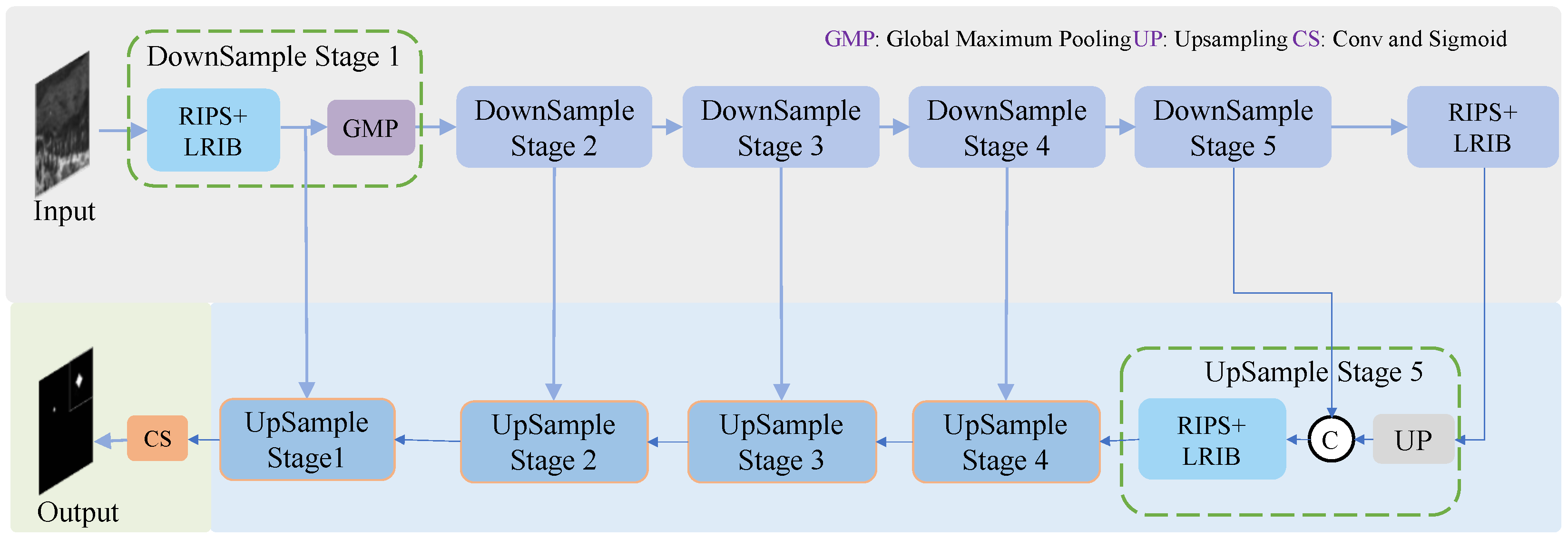
3.1. Overall Structure

As a baseline model in the field of image segmentation, U-Net has been widely applied in various semantic segmentation tasks due to its outstanding performance. U-Net uses a symmetric encoder–decoder architecture and connects them using skip connections. The encoder is responsible for downsampling the input image to reduce its resolution, after which the decoder restores the image to the corresponding resolution and concatenates it with the original image in the skip connection to restore the fine details in the image. This can make the network have various receptive fields and retains fine details in the image [25]. Therefore, the deep learning network we have designed utilizes the U-Net structure.

The overall structure of the network is as shown in Figure 1. The backbone of the network consists of RIPS and LRIB. The encoder contains a maximum pooling layer of size $2\times 2$ and step size 2, which reduces the height and width of the feature maps to half of their original size. In the decoder, in order to avoid the mismatch of feature maps caused by the fact that the height and width of the image are not divisible by 2, we use the bilinear interpolation method to scale the feature maps with small resolution to the corresponding size.

The structure of the encoder and decoder in U-Net is shown in Figure 2. The input feature map is passed through a $1\times 1$ convolutional layer to change its number of channels to the number of channels in the final output. After that, it will be split into two, one without any operation and one passing through the RIPS and LRIB modules. After that, these two paths are summed up and transported to the next module.

The output of the encoder is replicated into two, one input to the next encoder and one input to the corresponding upsampling stage through a skip connection, as shown in the bottom right corner of Figure 1. The feature map with small resolution is upsampled to obtain the feature map with large resolution, which is then concatenated with the feature map that has gone through the skip connection and fed into the decoder.

3.2. Residual Network with an Inverted Pyramid Structure

The size of the receptive field is very important in the image segmentation task. The image segmentation task is to classify each pixel in the image, so the larger the receptive field corresponding to each pixel, the more information the model can utilize to classify it. Thus, the larger the receptive field of the model, the better the image segmentation can be performed.

Currently, most deep learning algorithms increase the receptive field by stacking a large quantity of small convolutional layers. Using a large number of small-sized convolutional layers instead of a small number of large-sized convolutional layers can achieve the same theoretical receptive field and reduce the model’s parameter count. The effective receptive field of n convolutional layers of size k can be expressed in Equation (1). In this case, The required parameter count (PC) can be represented by Equation (2), where C represents the number of channels, which is taken as a fixed value. Therefore, when the receptive field is fixed, the parameter count is linearly related to the number of convolutional layers and linearly related to the square of the convolutional layer size. Therefore, using multiple small convolutional layers instead of large ones does reduce the number of parameters in the model.

$$RF=1+n(k-1)$$

(1)

$$PC=C^{2}n{k}^2$$

(2)

However, the effective receptive field of stacking small-size convolutional layers is actually smaller than that of a few large-size convolutional layers [26]. According to the characteristics of the effective receptive field, the influence factor within the receptive field rapidly decays with the distance from the center of the receptive field. The elements at the edge of the receptive field need to multiply by multiple sets of parameters to affect the final result, and the closer to the edge, the more parameter sets are needed. In addition, the elements at the edge of the receptive field have few paths to influence the final result, while the elements at the center of the receptive field can influence the final result through multiple paths. Therefore, the effective receptive field of a large number of small-size convolutional layers is far smaller than that of large-size convolutional layers.

We compare the actual effective receptive fields of convolutional blocks with the same theoretical receptive fields composed of convolutional layers of different sizes. The first is made up of 30 convolutional layers of size three, the second is made up of 15 convolutional layers of size five, and the third is made up of 10 convolutional layers of size seven. Their theoretical receptive fields are all 61, and the actual receptive fields on the $64\times 64$ picture are shown in Figure 3.

As can be observed from the figure, the actual receptive field of the blocks composed of multiple convolutional layers is smaller than the calculated theoretical receptive field, and the actual receptive field presents a two-dimensional Gaussian distribution, and the central pixel has a greater influence on the results, and the edge is smaller. At the same time, the actual receptive fields of the convolutional blocks composed of convolutional layers of size 3 and 7 are the smallest and largest, respectively, indicating that the actual receptive fields of the model can be effectively increased by increasing the size of the convolutional layers.

RIPS consists of several residual blocks, and its internal structure is shown in Figure 4. Each residual block consists of two convolutional layers of the same size with a normalization and an activation function. The size of the convolutional layer in the first residual block is Maxks, after which the size of the convolutional layer decreases and the size in the i-th residual block is Maxks-2i, and the size of the convolutional layer is fixed to 3 when the size of the convolutional layer is less than 3. This allows the network to obtain a large effective receptive field and to extract multiscale information.

Aiming to avoid the problem of excessive number of model parameters due to increasing the size of convolutional layers, we use depthwise separable convolution (DSC) to replace ordinary convolution with a kernel size greater than or equal to 7. DSC is commonly used in lightweight network models because of its ability to drastically reduce the number of parameters in the model. DSC consists of depthwise convolution and pointwise convolution. Each channel in depthwise convolution corresponds to one convolution kernel, so the number of convolution kernels is greatly reduced compared with ordinary convolution. The pointwise convolution is a normal convolution layer of size 1, which allows for the exchange of information between different channels.

The structure of the residual block using DSC and ordinary convolution is shown in Figure 5. While keeping the size of the convolutional kernel and the number of input and output channels constant, the number of parameters of DSC and ordinary convolution are shown in Equations (3) and (4), which shows that the number of parameters of ordinary convolution is proportional to the square of the number of channels, while the number of parameters of DSC is proportional to the number of channels, so it shows that the quantity of model parameters can be greatly reduced by using the DSC. When the size of the convolution layer is less than or equal to 5, the ordinary convolution layer is used.

For example, there is a convolutional layer with 32 channels and a convolutional kernel size of 7. When using a ordinary convolutional layer, the number of parameters is $32\times 32\times 7\times 7$ = 50,176, whereas the number of parameters using a depthwise separable convolution is $32\times 32+32\times 7\times 7$ = 2592. The number of parameters using an ordinary convolution is about 20 times the number of parameters using a DSC. In addition, when the number of channels in the convolutional layer is greater, the difference is even greater. Thus, by using DSC, the number of parameters in the model can be significantly reduced.

$$P{C}_{DSC}=C^2+C\times K{S}^2$$

(3)

$$P{C}_{Ord}=C^2\times K{S}^2$$

(4)

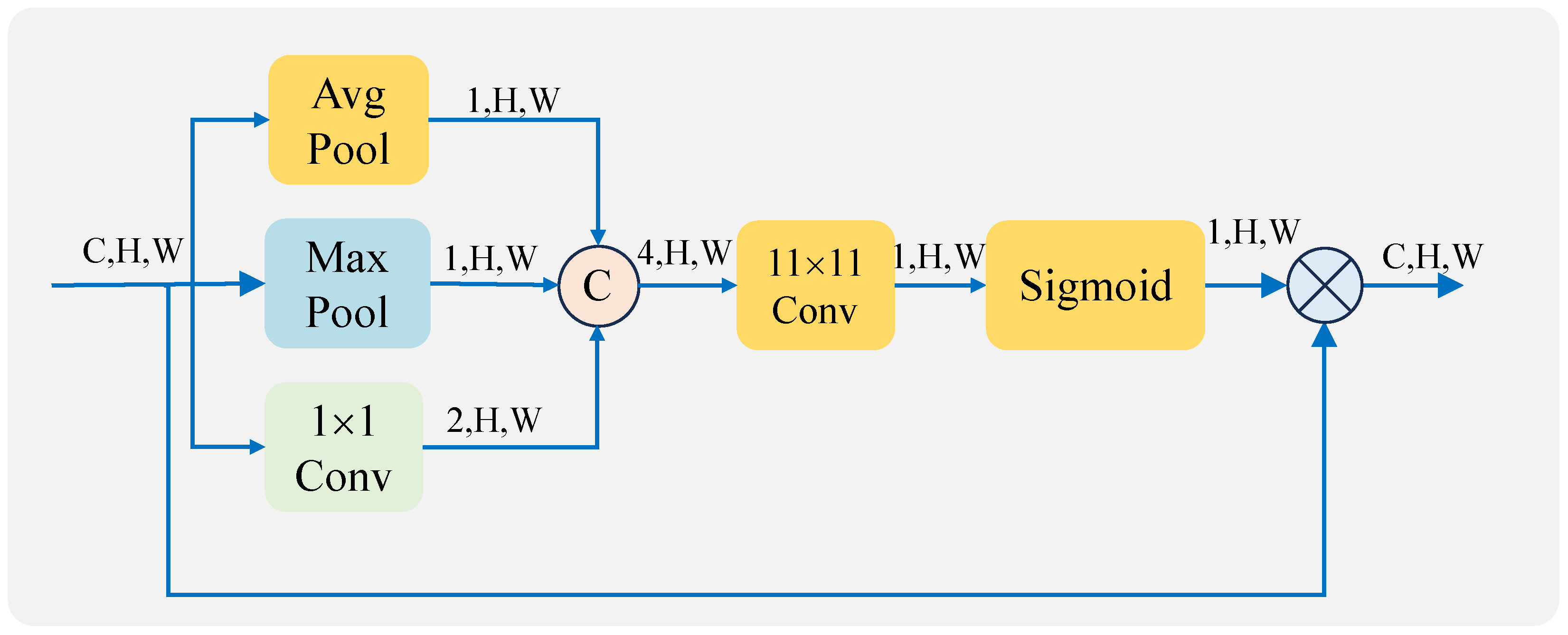
3.3. Attention Mechanism with Large-Size Receptive Field and Inverse Bottleneck Structure

The Transformer utilizes self-attention mechanisms to achieve a large receptive field, but its significant matrix computations and fully connected layers result in a substantial computational load and a large number of model parameters. In response to this, we have designed an attention mechanism with a large receptive field entirely based on convolutional layers. It consists of CHAM, SPAM, and an inverse bottleneck structure. Its structure is shown in Figure 6.

The CHAM involves average and max pooling in the spatial direction, followed by one-dimensional convolution to generate channel attention weights. Its detailed structure is shown in Figure 7. We use two different pooling operations to obtain two tensors, and after transposing, we obtain two tensors of shape $1\times 1\times C$, and concatenate the two tensors together. As a result, different feature information can be obtained.

The kernel size of this one-dimensional convolutional layer ($K{S}_{1D}$) is linearly related to the number of channels, as shown in Equation (5), where $int$ represents the rounding operation. Thus, it automatically adjusts the convolution kernel size based on the channels number, and when the number of channels increases, the size of the convolution kernel also increases. Thus, it is able to utilize more information to determine the location of more important channels, and therefore improves the detection effect of the model.

$$K{S}_{1D}=\left(int(C/20)\right)\times 2+1$$

(5)

The spatial attention involves pooling in the channel direction, followed by 2D convolution to generate spatial attention weights. Its detailed structure is shown in Figure 8. Through two different pooling operations and a $1\times 1$ convolutional layer, two $1\times H\times W$ and $2\times H\times W$ feature maps are generated, respectively, and then they are concatenated together to generate spatial weights through a convolutional layer.

The channel attention mechanism is able to give weight to the feature map in the channel domain, which can highlight the channels with more target information; while the spatial attention mechanism is able to give weight in the spatial domain, which can highlight the region where the target is located. The channel and spatial attention mechanisms are connected in tandem, so they can localize the channel and region where the target is located, which can help the model to better locate the target’s position.

By increasing the size of the convolutional layers within the attention mechanism, a larger receptive field can be achieved, and it can significantly reduce the required computation and storage consumption compared to the self-attention mechanism. This convolutional layer has a small number of input channels of 4 and an output channel of 1, so this convolutional layer uses an ordinary convolutional layer. In this paper, we have used a convolutional layer of size $11\times 11$ to extract spatial information.

Although the CHAM and SPAM are able to give different weights to different regions in the channel and spatial dimensions, respectively, they do not have the information interaction between channels. In addition, there are many depth-separable convolutions used in RIPS, and information exchange between channels is lacking.

So after channel and spatial attention, we introduce an inverse bottleneck structure. It is composed of two layers of convolution of size $1\times 1$ and two activation functions. After the first convolutional layer, the number of channels in the feature map becomes four times the original number of channels. After the second convolutional layer, the channel number returns to the original channel number. The information in different channels in the feature map can be exchanged by the $1\times 1$ convolutional layer, and its activation function can also increase the non-linearity of the model and improve the expressive power of the model. The reverse bottleneck structure enhances information propagation, enabling the network to capture more information.

3.4. Loss Function

Since infrared weak targets account for very few pixels in an infrared image, there is a serious positive and negative sample imbalance problem when using image segmentation methods for infrared weak target detection. If left unconstrained, the model will tend to predict all of the image as negative samples, which will reduce the detection probability significantly [27].

Therefore, we chose the loss function that can address the above problem for training the network. We adopt Focal Loss and Dice Loss as the loss function of the model. When calculating the value of the loss function, a larger weight can be added to the positive samples to increase their proportion in the loss function, so that the model can tend to learn more features of the positive samples.

Dice Loss (DL) [28] computes the loss only in the areas between the intersection of the predicted image and the actual image, and is therefore independent of the amount of positive and negative samples in the whole image, thus avoiding the problem of too many negative samples in the infrared image. A form of DL is computed as shown in Equation (6):

$$DiceLoss=1-{\displaystyle \frac{2TP+s}{2TP+FP+FN+s}}$$

(6)

where TP stands for true positives, FP stands for false positives, FN stands for false negatives, and s is taken as a value of 1 $\times {10}^{-5}$ to prevent the denominator from going to zero.

Focal Loss (FL) [29] adds large weights to the positive samples, which can make the positive and negative samples account for roughly the same percentage of losses. The calculation of FL is presented in Equation (7).

$$FocalLoss=-\alpha {(1-p)}^{\gamma }ylg\left(p\right)-(1-\alpha )(1-y)p^{\gamma }lg(1-p)$$

(7)

$\alpha$ is an adjustable parameter that is used to adjust the percentage of the samples in the loss function. $\gamma$ is a moderator that is used to control the weights of the easily classified and difficult to classify samples. p represents the result of the model’s prediction, and when p is close to 0 or 1, it means that the sample is easy to classify. y represents the actual classification of the labeling; when y is 1, it means that the sample is a target, and on the contrary, it means that it belongs to the background.

In order to combine the advantages of these two loss functions, we use their sum as the loss function of the model, which is shown in Equation (8).

$$Loss=DL+FL.$$

(8)

4. Experiments

4.1. Datasets and Implementation Details

We have chosen three IDST datasets: SIRST [12], MFIRST [30], and IRSTD-1k [31]. On these three datasets, we performed ablation experiments on the algorithm of this paper and comparison experiments with other algorithms. Our networks are all built on Pytorch’s framework and the networks were trained and tested on an NVIDIA RTX A6000 (48 GB memory). For training, we choose Adam as the optimizer of the model, so it is able to achieve good training results in most scenarios. In addition, the learning rate during training is 1 $\times {10}^{-5}$ and the epoch is 100.

MFIRST is a synthetic IDST detection dataset. It is generated by real IDSTs or targets generated by 2D Gaussian function, randomly overlaid onto high-resolution infrared images. It has a training set of 10,000 images and the image sizes are all $128\times 128$. It has a test set of 100 images with variable image sizes. The image size of this dataset is small and the number of images in the training set is large, so the batch size for training on this dataset is taken as 32.

SIRST is a publicly released infrared dim small target detection dataset. A number of these targets are very faint and easily submerged in complex backgrounds, about 55 percent of the targets are within 0.02 percent of the total image area, and only 35 percent of the targets have the maximum gray value. SIRST is divided into a training set with 322 images and a test set with 85 images. The image size in this dataset is not fixed, the image size is scaled to a uniform size of $320\times 320$ during training, and the batch size is taken as 8.

IRSTD-1k is a real IDST detection dataset. Its images are composed of small targets at different locations captured by an infrared camera from a long imaging distance under real-world conditions. The IRSTD-1k dataset has 1001 images of size $512\times 512$, divided into a training set with 901 images and a test set with 100 images. During training, the batch size was taken as 8.

4.2. Evaluation Metrics

The PD and FA evaluate the accuracy of the algorithm in detecting targets, and the Intersection over Union (IoU) evaluates the overlap between the predicted target region and the actual labeled region. When calculating these three metrics, the threshold is fixed at 0.5. We choose PD, FA, and IoU using fixed thresholds, and ROC curves using dynamic thresholds as evaluation metrics for comparing the effectiveness of detection.

The PD shows how many targets the model is able to detect and is the ratio of the amount of correctly detected targets $T_{correct}$ to the amount of actual targets $T_{act}$ in the annotation, which is calculated as shown in Equation (9).

$$PD={\displaystyle \frac{T_{correct}}{T_{act}}}$$

(9)

FA demonstrates how much of the background is recognized as a target by the algorithm and is the ratio of the total number of false target pixels $P_{false}$ to the total number of pixels in the entire image $P_{All}$. It is calculated as shown in Equation (10):

$$FA={\displaystyle \frac{P_{false}}{P_{All}}}$$

(10)

IoU describes the level of overlap between the model predictions and the actual labeled targets. It has a value from 0 to 1, where 0 indicates that a wrong target position is predicted and 1 indicates that the predicted and actual targets have exactly the same shape and position. It is computed as shown in Equation (11).

$$IoU={\displaystyle \frac{TP}{TP+FP+FN}}.$$

(11)

The ROC curve can show the detection result of the algorithm under changing thresholds. Its horizontal and vertical coordinates are the True Positive Rate (TPR) and the False Positive Rate (FPR), respectively. The larger the area covered under the curve, the better the algorithm’s detection effect. The TPR and FPR are computed by the following formulas:

$$\begin{array}{cc}\hfill & FPR={\displaystyle \frac{FP}{N}}\hfill \\ \hfill & TPR={\displaystyle \frac{TP}{N}}\hfill \end{array}$$

(12)

N is the number of pixels in the image.

4.3. Ablation Study

In order to validate the efficacy of the proposed algorithm, we performed ablation experiments on the above-mentioned datasets. We first compare the performance of models that use LRIB and have different Maxks in RIPS. After that, Maxks were fixed to be the best-performing Maxks, and the performance of models using different attention mechanisms was compared. Afterwards, the modifications in each of the three modules will be removed to verify the impact of our proposed improvements on the model detection results.

First, we compared the performance of models using different sizes of convolutional layers; by changing the Maxks in the RIPS, the size of the convolutional layers can be altered. Then, we compare the performance of networks using different AMs to validate the impact of our proposed improvements regarding the AM on model performance. During the ablation experiments, we kept other parts of the model unchanged.

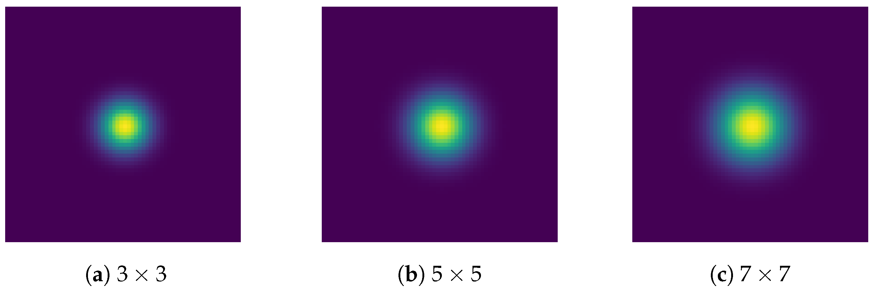
4.3.1. Comparison of Convolutional Layers of Different Sizes

In this part of the ablation experiments, we focus on verifying the effect of RIPS on the model performance. We compared the performance of models using different Maxks ranging from 5 to 13. In the process, we only changed the maximum convolutional layer size of the RIPS module and we kept the other modules the same. Their quantitative metrics on different datasets are shown in

Table 1. Comparison of quantitative metrics of the convolutional layers of different sizes on different datasets.

Maxks	Params/MB	MFIRST Dataset			SIRST Dataset			IRSTD-1k Dataset
		$\mathit{PD}$	$\mathit{FA}$	IoU	$\mathit{PD}$	$\mathit{FA}$	IoU	$\mathit{PD}$	$\mathit{FA}$	IoU
5	27.69	0.736	8.48 × 10−5	0.436	0.946	4.81 × 10−5	0.638	0.868	4.44 × 10−5	0.669
7	26.18	0.786	5.90 × 10−5	0.439	0.982	3.45 × 10−5	0.646	0.893	1.01 × 10−5	0.668
9	21.40	0.786	4.66 × 10−5	0.456	0.991	2.03 × 10−5	0.660	0.950	1.53 × 10−5	0.689
11	24.95	0.886	5.08 × 10−5	0.494	0.991	8.95 × 10−6	0.693	0.965	8.01 × 10−6	0.732
13	20.33	0.829	8.25 × 10−5	0.466	0.954	2.36 × 10−5	0.661	0.912	8.01 × 10−6	0.702

. Since the $PD$ is the number of detected targets over the total number of targets, the $PD$ is the same when the same number of targets are detected; so there are several different networks that achieved the same $PD$.

It is observed that, when the maximum convolution kernel size is less than 11, the performance of the model improves as the kernel size increases. However, when the kernel size increases to 13, the model’s performance declines, but still better than networks with maximum convolutional kernel sizes of 5 and 7. It is shown that increasing the size of the convolutional layer can increase the effective receptive field of the network and improve the performance of the model for detection, and that even if the size of the convolutional kernel is increased too much, it is still better than using a small-sized convolutional layer network for detection.

We also compared the parameter sizes of the different models, and from the table we can see that increasing the size of the convolutional layers did not increase the parameters, but in some cases reduced the number of parameters of the model, demonstrating that the number of parameters of the model can be effectively reduced by using depth-separable convolution.

4.3.2. Comparison of Networks Using Different Attention Mechanisms

We compare the detection performance of models using LRIB, Attention Mechanisms with Large Receptive Fields (AMLR), and CBAM with three different attention mechanisms. In the process, we only changed the AM used in the network, and the rest of the network remained consistent with the baseline model. Their quantitative metrics are shown in the

Table 2. Comparison of the performance of models using different attention mechanisms.

Attention Mechanism	MFIRST Dataset			SIRST Dataset			IRSTD-1k Dataset
	$\mathbf{PD}$	$\mathbf{FA}$	IoU	$\mathbf{PD}$	$\mathbf{FA}$	IoU	$\mathbf{PD}$	$\mathbf{FA}$	IoU
CBAM	0.857	6.71 × 10−5	0.465	0.912	5.86 × 10−6	0.656	0.894	3.45 × 10−6	0.661
AMLR	0.857	4.98 × 10−5	0.487	0.938	3.68 × 10−5	0.671	0.937	2.65 × 10−5	0.684
LRIB	0.886	5.08 × 10−5	0.494	0.991	8.95 × 10−6	0.693	0.965	8.01 × 10−6	0.732

.

Through the inverse bottleneck structure, the information between the channels can be fully exchanged, and it can increase the non-linearity of the model, which can better express the non-linear information, and thus can improve the detection effect of the model in different scenarios and improve the robustness of the model. It can be observed that the PD and FA of the model using LRIB are both superior to the model using AMLR. This shows that the inverse bottleneck structure in LRIB increases the exchange of information between different channels and retains more information, and can localize the target location better than AMLR, thus improving the detection accuracy of the model.

The PD and IoU of the network using LRIB on the three datasets exceeded those of the network using CBAM. It can be seen that, by increasing the receptive field of the AM, the AM can utilize more information in the image, thus giving a better weight to the feature map, and thus the critical regions can be more prominent, helping the model to detect the target.

4.4. Comparison with Other Advanced Algorithms

We have chosen multiple traditional and deep learning algorithms. Traditional algorithms include the filter-based algorithm FKRW [32], the HSV-based algorithm MPCM [33], and the data structure-based algorithm IPI [34]. Deep learning algorithms include MDvsFA [30] using generative adversarial networks, DNA-Net [8] with a large number of skip connections, ISTDU [35] using group convolution, LPNet [23] with global attention mechanism, MLCL [36] with local contrast, ACM [12], IAANet [37], ISNet [31], and AGPC [38].

The code for these compared algorithms is taken from their open source code and remains unchanged except for the training part. Each algorithm was trained on the above datasets, and the optimizer, learning rate, and other parameters used for training are consistent with our algorithms.

4.4.1. Quantitative Comparison

The comparison of quantifiable metrics of these algorithms on different datasets is shown in the

Table 3. Comparison of quantitative metrics of different algorithms on different datasets.

Method	Params/MB	MFIRST Dataset			SIRST Dataset			IRSTD-1k Dataset
		$\mathbf{PD}$	$\mathbf{FA}$	IoU	$\mathbf{PD}$	$\mathbf{FA}$	IoU	$\mathbf{PD}$	$\mathbf{FA}$	IoU
IPI	-	0.861	3.86 × 10−4	0.411	0.923	2.22 × 10−3	0.532	0.75	3.15 × 10−5	0.469
MPCM	-	0.828	9.58 × 10−3	0.402	0.945	1.30 × 10−2	0.120	0.956	6.09 × 10−3	0.483
FKRW	-	0.607	4.82 × 10−4	0.233	0.814	3.43 × 10−4	0.229	0.709	1.31 × 10−4	0.235
ISTDU	10.80	0.828	3.67 × 10−4	0.439	0.954	1.07 × 10−4	0.470	0.780	2.41 × 10−4	0.563
DNANet	54.26	0.692	2.35 × 10−4	0.351	0.889	2.63 × 10−4	0.464	0.815	1.84 × 10−5	0.611
MDvsFA	15.03	0.928	5.94 × 10−3	0.445	0.917	2.82 × 10−4	0.579	0.962	1.86 × 10−4	0.610
MLCL	6.44	0.478	9.46 × 10−5	0.251	0.565	1.65 × 10−5	0.350	0.808	2.81 × 10−5	0.616
LPNet	3.68	0.785	9.39 × 10−4	0.247	0.929	8.89 × 10−5	0.577	0.621	1.64 × 10−4	0.320
ACM	1.97	0.743	3.50 × 10−4	0.353	0.788	1.45 × 10−3	0.435	0.872	5.69 × 10−3	0.498
ISNet	4.21	0.700	1.69 × 10−5	0.482	0.859	7.87 × 10−5	0.459	0.886	4.47 × 10−5	0.541
IAANet	75.37	0.876	1.30 × 10−4	0.508	0.947	1.01 × 10−5	0.546	0.922	2.36 × 10−4	0.345
AGPC	47.33	0.607	2.12 × 10−5	0.322	0.823	3.72 × 10−5	0.538	0.829	1.74 × 10−4	0.411
Ours	24.95	0.886	1.08 × 10−5	0.494	0.991	8.95 × 10−6	0.693	0.965	8.01 × 10−6	0.732

. Among them, the higher the PD and IoU, the better, while the lower the FA, the better. The best metrics among these different algorithms are highlighted in red and bold font, and the second-best metrics are shown in blue font. Overall, due to the fact that deep learning algorithms are able to autonomously learn the most suitable weights and have stronger generalization ability, they generally outperform traditional algorithms.

MPCM calculates the grayscale difference between the target and the background in regions of different sizes, so it can adapt to scenes with targets of different sizes, resulting in a PD. However, it is very sensitive to rapidly changing backgrounds. When the center grayscale value of a region is higher than the surrounding grayscale values, the algorithm will mistakenly identify that region as the location of the target, leading to a high FA.

The IPI algorithm divides the image into overlapping image blocks using a sliding window, and then reconstructs them. It uses methods to solve sparse and low-rank matrices for object detection. It can be applied to scenes with complex backgrounds, hence achieving the best quantifiable metrics among traditional algorithms. However, it relies on the sparsity of the target for detection, so the detection performance deteriorates when there are multiple targets, resulting in poorer performance on datasets with a higher number of targets.

The FKRW algorithm uses mean and facet kernel filters to remove the background and then employs a random walk algorithm to segment the target and background. It can eliminate most of the background and interference, resulting in a low FA. However, in the process, some target information is inevitably removed, resulting in a relatively low PD.

Among the deep learning algorithms, MDvsFA achieved the highest PD in the MFIRST dataset and the second highest PD in the IRSTD-1k dataset, but it also had the highest FA on the three datasets. The MLCL algorithm achieves the second smallest FA in the SIRST dataset, but its PD on the MFIRST and SIRST datasets are also low. Due to the post-processing of LPNet, the image will be blurry. Therefore, its IoU on the MFIRST and IRSTD-1k datasets are the lowest among the compared deep learning algorithms. Therefore, MDvsFA, MLCL, and LPNet can not accurately detect the target in the image.

ISTDU achieved the second PD on the SIRST dataset, but did not perform well on other datasets. DNANet and ISNet achieved the second lowest FA on the IRSTD-1k and MFIRST datasets, respectively, but their other quantitative metrics were not good. The IAANet algorithm achieved the best IOU on the MFIRST dataset, but our algorithm outperformed the IAANet algorithm in other metrics. The quantitative metrics of ACM and AGPC are not too good and not too bad.

By using RIPS, the network can be made to have a large effective receptive field, which can allow the network to utilize more information to differentiate between targets and backgrounds, thus improving the detection effect of the model in complex backgrounds and reducing the false alarm rate of the model. In addition the different sizes of convolutional layers inside, its module can realize different sizes of receptive fields, thus enabling the model to acquire rich multi-scale information and improve the detection rate of the model.

By using LRIB, it has different pooling operations within it, so it is able to extract different feature information, and it has a large convolutional layer, which is able to achieve a large effective receptive field, so it is able to utilize more information to distinguish between the target and the background, so it is able to generate better weights, which helps the model to better detect the target.

Thanks to the large effective receptive fields brought by large convolutional kernels and the precise target localization brought by LRIB, our algorithm has achieved the best quantitative metrics among the compared algorithms. Our algorithm achieved the second best PD on the MFIRST dataset and the best results for all other metrics, which proves that the algorithm we designed achieves the best detection effect.

Additionally, we compared the ROC curve using dynamic thresholds, as shown in Figure 9, and it can be observed that our algorithm’s performance exceeds that of other algorithms under dynamic threshold testing conditions.

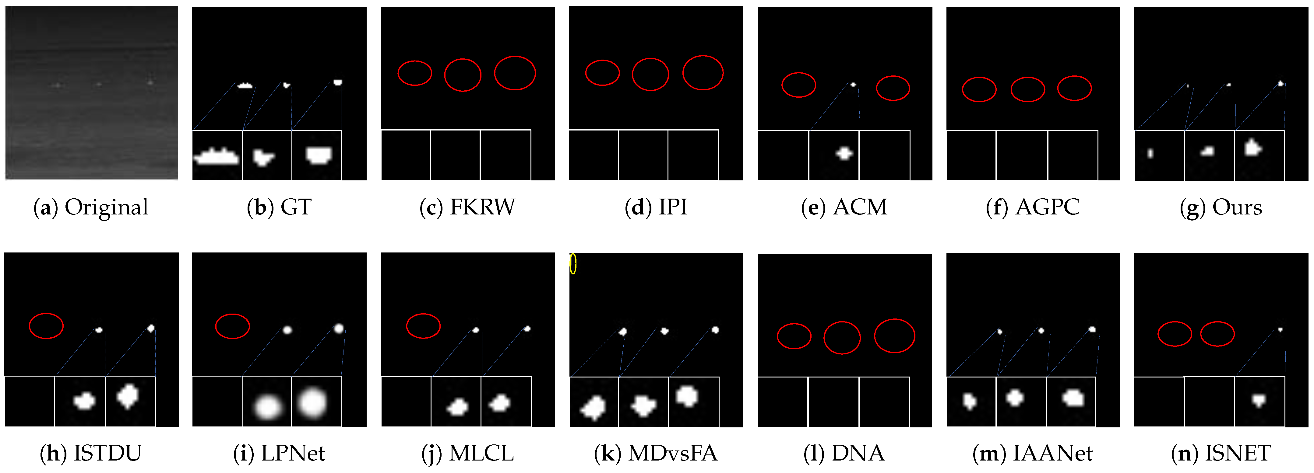
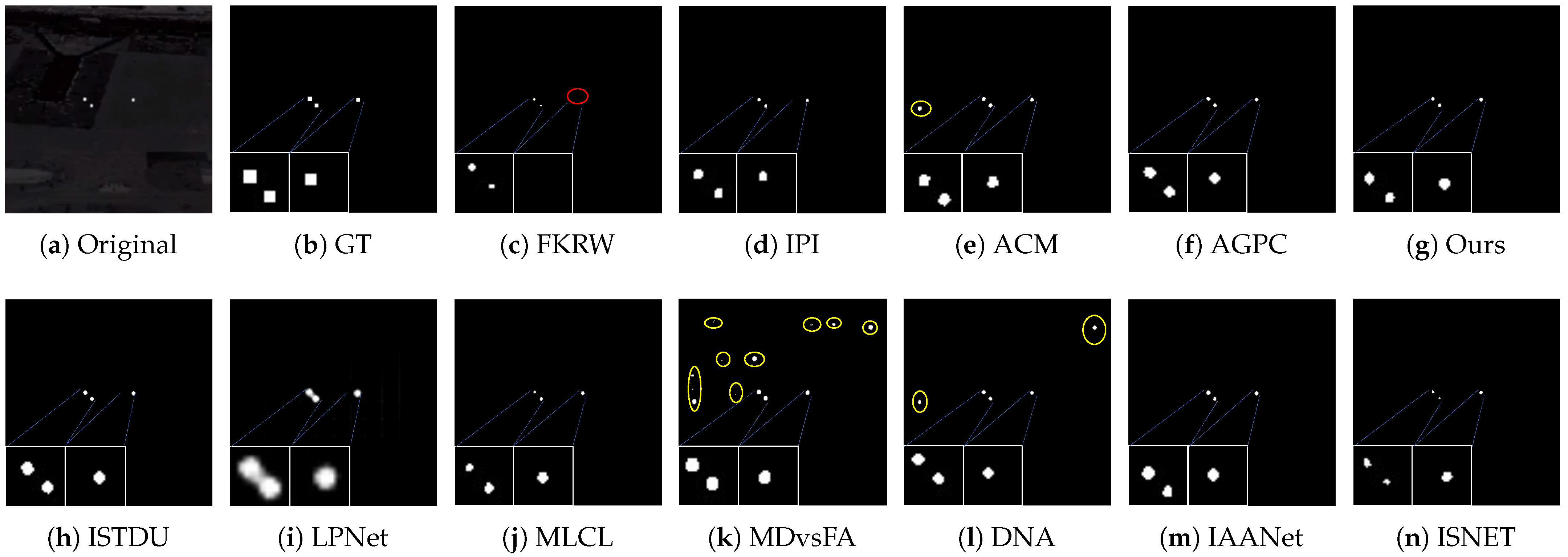
4.4.2. Visual Comparison

Some visual comparison images of each of the three datasets are shown in Figure 10, Figure 11, Figure 12, Figure 13, Figure 14 and Figure 15, where the yellow circles in the images represent false alarms and the red circles represent missed detections. We zoomed the target area at the corners of the image, and when the image contains multiple targets or false alarms, we used blue dotted lines to correspond the targets in the image to the zoomed picture.

Among the traditional algorithms, the IPI algorithm is able to detect all the targets, but there is a certain degree of false alarms, and it is the best detection effect among the traditional algorithms in a comprehensive view. FKRW has fewer false alarms, but it has a significant amount of leakage, and it introduces extra noise at the bottom edge of the image, which is not so good for the detection effect in a comprehensive view. MPCM is too sensitive to the noise, and there is a large number of false targets in its image and it is difficult to distinguish the location of the target. The detection effect of this algorithm is the worst among these algorithms, so the detection results of this algorithm are not shown.

MLCL has no false alarms, but many targets are not detected; mdfa has no leakage detection, but there are also many false alarms, so the detection effect of these two algorithms is not good. istdu has some leakage detection and false alarms, while dna has basically no leakage detection, and there are fewer false alarms, and the detection effect is satisfactory from a comprehensive point of view. LPnet has very few false alarms and leakage detections, but the subsequent processing will make the target’s detail information lost, resulting in the loss of the target’s information.

When the image background is complex, the ACM algorithm cannot effectively distinguish between the background and the target, resulting in a significant number of false alarms, and it cannot detect all the targets. AGPC cannot detect targets with low contrast and identify areas that are brighter than the target as targets, resulting in missed detections and false alarms.IAANet is able to detect all targets, but there are also false alarms. ISNet does not detect all the objects in the image with low contrast and many objects, and all other objects are accurately detected.

Our algorithm is able to detect all targets in the image with no false alarms, achieving the best detection results among the algorithms compared.

4.5. Discussion

Combining the above comparison of quantitative metrics and visual comparison, the detection performance of deep learning-based algorithms is significantly better than that of traditional algorithms. The traditional algorithm relies on the a priori knowledge summarized by people before, and when the images in the dataset do not conform to that a priori knowledge, the detection effect will be greatly reduced, so the traditional algorithm’s generalization ability is insufficient to meet the requirements of the actual scene. The algorithm based on deep learning can adapt to different datasets by changing the internal weights, so the generalization ability is stronger and the detection effect is better than the traditional algorithm.

By using large-size convolutional layers, our algorithm can have a large effective sensory field, which can improve the robustness of the model and improve the detection effect. By using LRIB, it can enable the algorithm to better localize the region where the target is located. Compared to other algorithms, our algorithm achieves the best quantization metrics and also the best detection results. Through the ablation and comparison experiments, it can be seen that our proposed RIPS and LRIB can effectively boost the detection results of the model.

5. Conclusions

In this article, we designed an IDST detection algorithm LRFNet with a large receptive field. It uses residual network with an inverted pyramid structure. Therefore, it can enable the network to have a larger effective receptive field, thereby enabling the network to extract more information. In addition, it uses the attention mechanism with a large-size receptive field and inverse bottleneck structure, which can retain more information and improve the positioning accuracy of the model through the reverse bottleneck structure. Our LRFNet outperforms other advanced algorithms on different datasets, proving the progressiveness of our algorithm.

Although our algorithm outperforms all other algorithms on all other datasets, our algorithm does not achieve the best quantitative metrics on the MFIRST dataset. Therefore, we propose to continue to improve the network to improve the detection of the model. In addition, the scenarios we have applied so far are all general remote sensing scenarios, and in the future we will also try to adapt the space remote sensing scenarios and test on that scenario.

References

1. Ma, T.; Yang, Z.; Liu, B.; Sun, S. A Lightweight Infrared Small Target Detection Network Based on Target Multiscale Context. IEEE Geosci. Remote Sens. Lett. 2023, 20, 7000305. [Google Scholar] [CrossRef]
2. Rawat, S.S.; Verma, S.K.; Kumar, Y. Review on recent development in infrared small target detection algorithms. Procedia Comput. Sci. 2020, 167, 2496–2505. [Google Scholar] [CrossRef]
3. Zhao, M.; Li, W.; Li, L.; Hu, J.; Ma, P.; Tao, R. Single-Frame Infrared Small-Target Detection: A survey. IEEE Geosci. Remote Sens. Mag. 2022, 10, 87–119. [Google Scholar] [CrossRef]
4. Hu, Z.; Su, Y. An infrared dim and small target image preprocessing algorithm based on improved bilateral filtering. In Proceedings of the 2021 International Conference on Computer, Blockchain and Financial Development (CBFD), Nanjing, China, 23–25 April 2021; pp. 74–77. [Google Scholar] [CrossRef]
5. Han, J.; Ma, Y.; Zhou, B.; Fan, F.; Liang, K.; Fang, Y. A Robust Infrared Small Target Detection Algorithm Based on Human Visual System. IEEE Geosci. Remote Sens. Lett. 2014, 11, 2168–2172. [Google Scholar] [CrossRef]
6. Wan, M.; Gu, G.; Xu, Y.; Qian, W.; Ren, K.; Chen, Q. Total Variation-Based Interframe Infrared Patch-Image Model for Small Target Detection. IEEE Geosci. Remote Sens. Lett. 2022, 19, 7003305. [Google Scholar] [CrossRef]
7. Zhao, B.; Wang, C.; Fu, Q.; Han, Z. A Novel Pattern for Infrared Small Target Detection with Generative Adversarial Network. IEEE Trans. Geosci. Remote Sens. 2021, 59, 4481–4492. [Google Scholar] [CrossRef]
8. Li, B.; Xiao, C.; Wang, L.; Wang, Y.; Lin, Z.; Li, M.; An, W.; Guo, Y. Dense Nested Attention Network for Infrared Small Target Detection. IEEE Trans. Image Process. 2023, 32, 1745–1758. [Google Scholar] [CrossRef]
9. Ma, T.; Yang, Z.; Wang, J.; Sun, S.; Ren, X.; Ahmad, U. Infrared Small Target Detection Network with Generate Label and Feature Mapping. IEEE Geosci. Remote Sens. Lett. 2022, 19, 6505405. [Google Scholar] [CrossRef]
10. Shelhamer, E.; Long, J.; Darrell, T. Fully Convolutional Networks for Semantic Segmentation. IEEE Trans. Pattern Anal. Mach. Intell. 2017, 39, 640–651. [Google Scholar] [CrossRef]
11. Ronneberger, O.; Fischer, P.; Brox, T. U-Net: Convolutional Networks for Biomedical Image Segmentation. In Proceedings of the Medical Image Computing and Computer-Assisted Intervention—MICCAI 2015, Munich, Germany, 5–9 October 2015; Navab, N., Hornegger, J., Wells, W.M., Frangi, A.F., Eds.; Springer: Cham, Switzerland, 2015; pp. 234–241. [Google Scholar]
12. Dai, Y.; Wu, Y.; Zhou, F.; Barnard, K. Asymmetric Contextual Modulation for Infrared Small Target Detection. In Proceedings of the 2021 IEEE Winter Conference on Applications of Computer Vision (WACV), Waikoloa, HI, USA, 3–8 January 2021; pp. 949–958. [Google Scholar] [CrossRef]
13. Ding, X.; Zhang, X.; Han, J.; Ding, G. Scaling Up Your Kernels to 31 × 31: Revisiting Large Kernel Design in CNNs. In Proceedings of the 2022 IEEE/CVF Conference on Computer Vision and Pattern Recognition (CVPR), New Orleans, LA, USA, 18–24 June 2022; pp. 11953–11965. [Google Scholar] [CrossRef]
14. Liu, Z.; Mao, H.; Wu, C.Y.; Feichtenhofer, C.; Darrell, T.; Xie, S. A ConvNet for the 2020s. In Proceedings of the 2022 IEEE/CVF Conference on Computer Vision and Pattern Recognition (CVPR), New Orleans, LA, USA, 18–24 June 2022; pp. 11966–11976. [Google Scholar] [CrossRef]
15. Lin, F.; Bao, K.; Li, Y.; Zeng, D.; Ge, S. Learning Contrast-Enhanced Shape-Biased Representations for Infrared Small Target Detection. IEEE Trans. Image Process. 2024, 33, 3047–3058. [Google Scholar] [CrossRef]
16. Brauwers, G.; Frasincar, F. A General Survey on Attention Mechanisms in Deep Learning. IEEE Trans. Knowl. Data Eng. 2023, 35, 3279–3298. [Google Scholar] [CrossRef]
17. Hu, J.; Shen, L.; Sun, G. Squeeze-and-Excitation Networks. In Proceedings of the 2018 IEEE/CVF Conference on Computer Vision and Pattern Recognition, Salt Lake City, UT, USA, 18–23 June 2018; pp. 7132–7141. [Google Scholar] [CrossRef]
18. Jaderberg, M.; Simonyan, K.; Zisserman, A.; Kavukcuoglu, K. Spatial transformer networks. In Proceedings of the 28th International Conference on Neural Information Processing Systems, NIPS’15, Montreal, QC, Canada, 7–12 December 2015; Volume 2, pp. 2017–2025. [Google Scholar]
19. Woo, S.; Park, J.; Lee, J.Y.; Kweon, I.S. CBAM: Convolutional Block Attention Module. In Proceedings of the Computer Vision—ECCV 2018, Munich, Germany, 8–14 September 2018; Ferrari, V., Hebert, M., Sminchisescu, C., Weiss, Y., Eds.; Springer: Cham, Switzerland, 2018; pp. 3–19. [Google Scholar]
20. Vaswani, A.; Shazeer, N.; Parmar, N.; Uszkoreit, J.; Jones, L.; Gomez, A.N.; Kaiser, L.; Polosukhin, I. Attention is all you need. In Proceedings of the 31st International Conference on Neural Information Processing Systems, NIPS’17, Long Beach, CA, USA, 4–9 December 2017; pp. 6000–6010. [Google Scholar]
21. Han, K.; Wang, Y.; Chen, H.; Chen, X.; Guo, J.; Liu, Z.; Tang, Y.; Xiao, A.; Xu, C.; Xu, Y.; et al. A Survey on Vision Transformer. IEEE Trans. Pattern Anal. Mach. Intell. 2023, 45, 87–110. [Google Scholar] [CrossRef]
22. Chung, W.Y.; Lee, I.H.; Park, C.G. Lightweight Infrared Small Target Detection Network Using Full-Scale Skip Connection U-Net. IEEE Geosci. Remote Sens. Lett. 2023, 20, 7000705. [Google Scholar] [CrossRef]
23. Chen, F.; Gao, C.; Liu, F.; Zhao, Y.; Zhou, Y.; Meng, D.; Zuo, W. Local Patch Network with Global Attention for Infrared Small Target Detection. IEEE Trans. Aerosp. Electron. Syst. 2022, 58, 3979–3991. [Google Scholar] [CrossRef]
24. Wang, Z.; Yang, J.; Pan, Z.; Liu, Y.; Lei, B.; Hu, Y. APAFNet: Single-Frame Infrared Small Target Detection by Asymmetric Patch Attention Fusion. IEEE Geosci. Remote Sens. Lett. 2023, 20, 7000405. [Google Scholar] [CrossRef]
25. Siddique, N.; Paheding, S.; Elkin, C.P.; Devabhaktuni, V. U-Net and Its Variants for Medical Image Segmentation: A Review of Theory and Applications. IEEE Access 2021, 9, 82031–82057. [Google Scholar] [CrossRef]
26. Luo, W.; Li, Y.; Urtasun, R.; Zemel, R. Understanding the effective receptive field in deep convolutional neural networks. In Proceedings of the 30th International Conference on Neural Information Processing Systems, NIPS’16, Barcelona, Spain, 5–10 December 2016; pp. 4905–4913. [Google Scholar]
27. Wei, W.; Ma, T.; Li, M.; Zuo, H. Infrared Dim and Small Target Detection Based on Superpixel Segmentation and Spatiotemporal Cluster 4D Fully-Connected Tensor Network Decomposition. Remote Sens. 2024, 16, 34. [Google Scholar] [CrossRef]
28. Li, X.; Sun, X.; Meng, Y.; Liang, J.; Wu, F.; Li, J. Dice Loss for Data-imbalanced NLP Tasks. arXiv 2019, arXiv:1911.02855. [Google Scholar]
29. Lin, T.Y.; Goyal, P.; Girshick, R.; He, K.; Dollár, P. Focal Loss for Dense Object Detection. In Proceedings of the 2017 IEEE International Conference on Computer Vision (ICCV), Venice, Italy, 22–29 October 2017; pp. 2999–3007. [Google Scholar] [CrossRef]
30. Wang, H.; Zhou, L.; Wang, L. Miss Detection vs. False Alarm: Adversarial Learning for Small Object Segmentation in Infrared Images. In Proceedings of the 2019 IEEE/CVF International Conference on Computer Vision (ICCV), Seoul, Republic of Korea, 27 October–2 November 2019; pp. 8508–8517. [Google Scholar] [CrossRef]
31. Zhang, M.; Zhang, R.; Yang, Y.; Bai, H.; Zhang, J.; Guo, J. ISNet: Shape Matters for Infrared Small Target Detection. In Proceedings of the 2022 IEEE/CVF Conference on Computer Vision and Pattern Recognition (CVPR), New Orleans, LA, USA, 18–24 June 2022; pp. 867–876. [Google Scholar] [CrossRef]
32. Qin, Y.; Bruzzone, L.; Gao, C.; Li, B. Infrared Small Target Detection Based on Facet Kernel and Random Walker. IEEE Trans. Geosci. Remote Sens. 2019, 57, 7104–7118. [Google Scholar] [CrossRef]
33. Wei, Y.; You, X.; Li, H. Multiscale patch-based contrast measure for small infrared target detection. Pattern Recognit. 2016, 58, 216–226. [Google Scholar] [CrossRef]
34. Gao, C.; Meng, D.; Yang, Y.; Wang, Y.; Zhou, X.; Hauptmann, A.G. Infrared Patch-Image Model for Small Target Detection in a Single Image. IEEE Trans. Image Process. 2013, 22, 4996–5009. [Google Scholar] [CrossRef] [PubMed]
35. Hou, Q.; Zhang, L.; Tan, F.; Xi, Y.; Zheng, H.; Li, N. ISTDU-Net: Infrared Small-Target Detection U-Net. IEEE Geosci. Remote Sens. Lett. 2022, 19, 7506205. [Google Scholar] [CrossRef]
36. Yu, C.; Liu, Y.; Wu, S.; Hu, Z.; Xia, X.; Lan, D.; Liu, X. Infrared small target detection based on multiscale local contrast learning networks. Infrared Phys. Technol. 2022, 123, 104107. [Google Scholar] [CrossRef]
37. Wang, K.; Du, S.; Liu, C.; Cao, Z. Interior Attention-Aware Network for Infrared Small Target Detection. IEEE Trans. Geosci. Remote Sens. 2022, 60, 5002013. [Google Scholar] [CrossRef]
38. Zhang, T.; Li, L.; Cao, S.; Pu, T.; Peng, Z. Attention-Guided Pyramid Context Networks for Detecting Infrared Small Target Under Complex Background. IEEE Trans. Aerosp. Electron. Syst. 2023, 59, 4250–4261. [Google Scholar] [CrossRef]
Figure 1. LRF-Net structure.
Remotesensing 17 00307 g001
Figure 2. Schematic of encoders and decoders using RIPS and LIRB.
Remotesensing 17 00307 g002
Figure 3. The actual effective receptive field of convolutional blocks with the same theoretical receptive field composed of convolutional layers of different sizes.
Remotesensing 17 00307 g003
Figure 4. Schematic representation of the internal structure of RIPS and the structure of the residual blocks used.
Remotesensing 17 00307 g004
Figure 5. Schematic diagram of residual blocks using depthwise separable convolutions and ordinary convolutions.
Remotesensing 17 00307 g005
Figure 6. Schematic representation of the attention mechanism with a large receptive field and an inverse bottleneck structure.
Remotesensing 17 00307 g006
Figure 7. Channel attention structure.
Remotesensing 17 00307 g007
Figure 8. Schematic structure of the spatial attention mechanism.
Remotesensing 17 00307 g008
Figure 9. ROC curves of different algorithms. The ROC performance of IPI and MPCM is too poor to be shown in the figure. (a) ROC curves of different algorithms on the MFIRST dataset. (b) ROC curves of different algorithms on the SIRST dataset. (c) ROC curves of different algorithms on the IRSTD-1k dataset.
Remotesensing 17 00307 g009
Figure 10. Visual example of some representative methods in the MFIRST dataset.
Remotesensing 17 00307 g010
Figure 11. Examples of visual comparisons of methods in the MFIRST dataset.
Remotesensing 17 00307 g011
Figure 12. Examples of visual comparisons of methods in the SIRST dataset.
Remotesensing 17 00307 g012
Figure 13. Examples of visual comparisons of methods in the SIRST dataset.
Remotesensing 17 00307 g013
Figure 14. Examples of visual comparisons of methods in the IRSTD-1k dataset.
Remotesensing 17 00307 g014
Figure 15. Visual example of some representative methods in the IRSTD-1k dataset.
Remotesensing 17 00307 g015