Abstract
With traditional three-dimensional (3-D) reconstruction methods for space targets, it is difficult to achieve 3-D structure and attitude reconstruction simultaneously. To tackle this problem, a 3-D reconstruction method for space targets is proposed, and the alignment and fusion of optical and ISAR images are investigated. Firstly, multiple pairs of optical and ISAR images are acquired in the joint optical-and-ISAR co-location observation system (COS). Then, key points of space targets on the images are used to solve for the Doppler information and the 3-D attitude. Meanwhile, the image offsets of each pair are further aligned based on Doppler co-projection between optical and ISAR images. The 3-D rotational offset relationship and the 3-D translational offset relationship are next deduced to align the spatial offset between pairs of images based on attitude changes in neighboring frames. Finally, a voxel trimming mechanism based on growth learning (VTM-GL) is designed to obtain the reserved voxels where mask features are used. Experimental results verify the effectiveness and robustness of the OC-V3R-OI method.
1. Introduction
Optical imaging and inverse synthetic aperture radar (ISAR) imaging are extensively used for space target monitoring to obtain two-dimensional (2-D) images [1,2]. The 2-D image is actually the projection of the three-dimensional (3-D) structure. The compression and downscaling of 3-D information make it difficult to provide a comprehensive description of the target [3,4]. It is obvious that 3-D information is necessary if more accurate spacecraft monitoring, target identification, and behavioral judgement is to be achieved [5,6]. The target maintains a triaxial stabilized attitude during normal operation, allowing the 3-D reconstruction to be achieved by utilizing sequential images [7]. However, the total image view angle is limited for a single observation arc, resulting in poor 3-D reconstruction performance. When the space target is out of control or in an attitude adjustment state, the target is often rotating slowly or non-stably [8,9,10], increasing the imaging view angle, and the viewpoint information is relative abundant. In this case, the attitudes of the target model are unknown at different observation moments, and the projection relationship is difficult to solve. Therefore, in order to accommodate space targets in different scenarios, the generalized 3-D reconstruction method should be independent of the target’s attitude variation. Meanwhile, the 3-D structure and attitude can be reconstructed simultaneously.
Optical image-based 3-D reconstruction methods are mainly derived from multi-view 3-D reconstruction [11], which focuses on the extraction and trajectory association of feature points from multi-angle images. Typically, in such methods, the attitude of the target is often unknown. Therefore, optical flow methods are applied for feature extraction and tracking by matching cameras between consecutive frames to generate the 3-D structure. Then, the six-degree iterative closest point (6D-ICP) method is used to estimate the attitude and structure [12]. However, the poor lighting conditions of space targets results in few robustly extracted feature points, making the reconstruction point cloud sparse. Consequently, camera poses and prior component shapes are introduced [11]. Meanwhile, the sparse point cloud and the prior component shape constraint of the space targets are used to recover the real dense point cloud. However, this relies on the completeness of the prior component library, and it is difficult to adapt it to situations such as defective deformation of components.
ISAR-image-based 3-D reconstruction algorithms can be classified according to the number of channels and are mainly divided into two classes, i.e., multi-channel-based methods and single-channel-based methods. Actually, multi-channel-based methods utilize interferometric inverse synthetic aperture radar (InISAR) processing [13,14,15]. However, the hardware requirements of the InISAR imaging methods are high and costly. Therefore, single-channel-based methods have been widely studied for several years. These methods require prolonged observation of space targets to obtain a multi-view image sequence. Then, cross-range scaling [16,17] is used for individual images, and scatter point trajectory association [18,19] is used for all sequenced images. Subsequently, the random sample consensus (RANSAC) method is utilized in [20,21] to remove the falsely matched points, and then the 3-D reconstruction is completed based on factorization decomposition theory [22,23]. However, due to the signal noise and anisotropy of electromagnetic scattering characteristics, it is challenging to stably extract and correlate scattering points from sequential images, resulting in a sparse reconstructed point cloud. To avoid the processing of scattering center extraction and trajectory association, energy accumulation was proposed in [7]. This method resolves the projection matrix based on line of sight (LOS) and reconstructs each point using a particle swarm optimization (PSO) algorithm. However, the targets need to be triaxially stabilized space targets. Subsequently, a method was proposed for reconstructing rotating targets in [24]. Furthermore, an extended factorization framework (EFF) was proposed [25]. This method solved the projection matrix by applying the factorization decomposition on the trajectory matrix of several extracted key points. Then, an energy-accumulation-based reconstruction method was used to solve the 3-D scattering candidate points for any moving target, as in [7]. However, this reconstructed 3-D structure is defined in the target coordinate system, making it impossible to obtain the target attitude. Recently, deep-learning-based 3-D reconstruction methods for ISAR image sequences have also shown better performance and do not require correlated scattering points of ISAR image sequences [26]. The method is also limited by the type of target motion and has a long training time.
Optical and ISAR images differ in their imaging mechanisms and have both been investigated in the field of space target attitude estimation [27,28]. Both of these methods provide a basic description of the co-location observation system (COS) for the joint optical-and-ISAR method. Motivated by these works, the concept of utilizing multi-sensor joint observation scenes can be extended to the method of 3-D reconstruction. A 3-D reconstruction method was proposed by Zhou et al. [29], which for the first time utilized both optical and ISAR images and obtained dense reconstruction results using a voxel-based 3-D representation. However, the method can only be applied to three-axis-stable space targets. Then, Long et al. proposed a co-location fusion of ISAR and optical images for 3-D reconstruction, which can simultaneously obtain the 3-D structure and attitude of a rotating target. However, the image and space offsets were not taken into account [30].
Aiming at the above problems, an offset correction and voxel-based 3D reconstruction method using optical and ISAR images (OC-V3R-OI) is proposed based on the optical and ISAR image alignment and fusion. Initial work about offset correction has been shown in [31], and further research will be presented in this paper. Firstly, the joint optical-and-ISAR COS is constructed to obtain multiple pairs of optical images and ISAR images. To obtain a precise description of the target on the images, image features are extracted. Subsequently, the key point features are applied for image offset correction and spatial offset correction, taking into account the offsets in each pair of images and the differences in attitude and position of the targets between adjacent pairs of images. Further, mask features are utilized in the voxel trimming mechanism based on growth learning (VTM-GL) processing. In the above processing, the target attitude information can be acquired simultaneously. Finally, 3-D voxels of the space targets are acquired. The main contributions of this paper are as follows:
- Accurate theoretical models for image offset correction and spatial offset correction: The OC-V3R-OI method starts from the imaging mechanism, and derives detailed analytical expressions for image offset correction and spatial offset correction. This facilitates more accurate 3-D reconstruction and provides substantial support for other situational awareness tasks in this scenario.
- Independence with regard to the prior motion information: The OC-V3R-OI method is independent of the prior motion information, and the corresponding model attitude at each imaging frame can be given during the observation time. This capability makes the OC-V3R-OI method suitable for targets with unknown motion types and enhances its applicability.
- Accurate voxel trimming mechanism: To increase the robustness of the OC-V3R-OI method, the VTM-GL method was deliberately designed to enable the voxel trimming mechanism to dynamically remove and add voxels, thereby ensuring high reconstruction accuracy and optimizing the utilization of available information.
This article is organized as follows. Section 2 establishes the joint optical-and-ISAR COS, while Section 3 details the key modules of the OC-V3R-OI method. Section 4 presents the detailed algorithmic flow of the OC-V3R-OI method, including the required inputs, the expected outputs, and the specific steps involved in the algorithm. In Section 5, experimental results utilizing electromagnetic simulation data demonstrate the effectiveness of the OC-V3R-OI method. Section 6 provides an analysis of the experimental results, and Section 7 draws the final conclusions.
2. Principals of Optical-and-ISAR Co-Location System
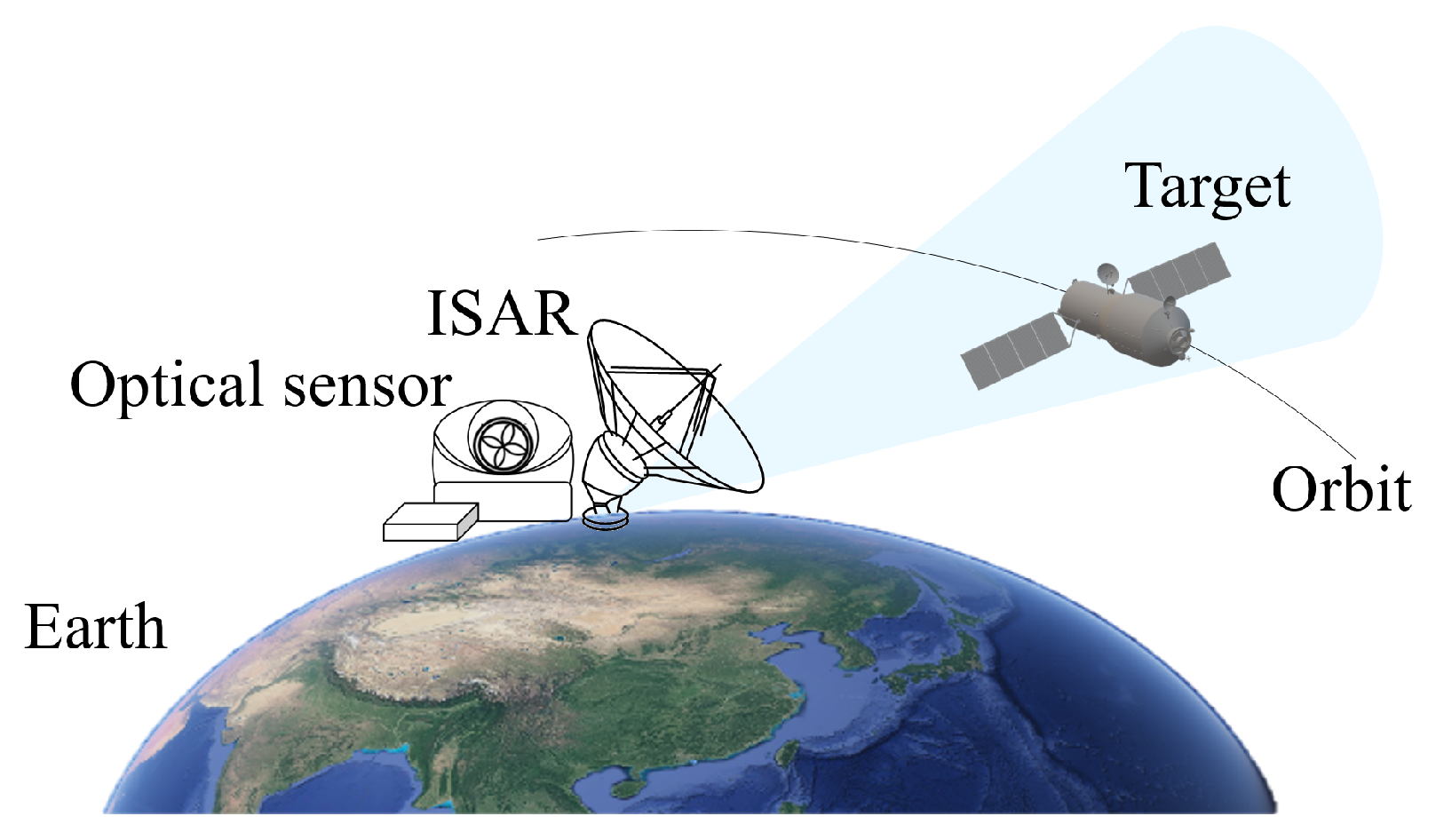
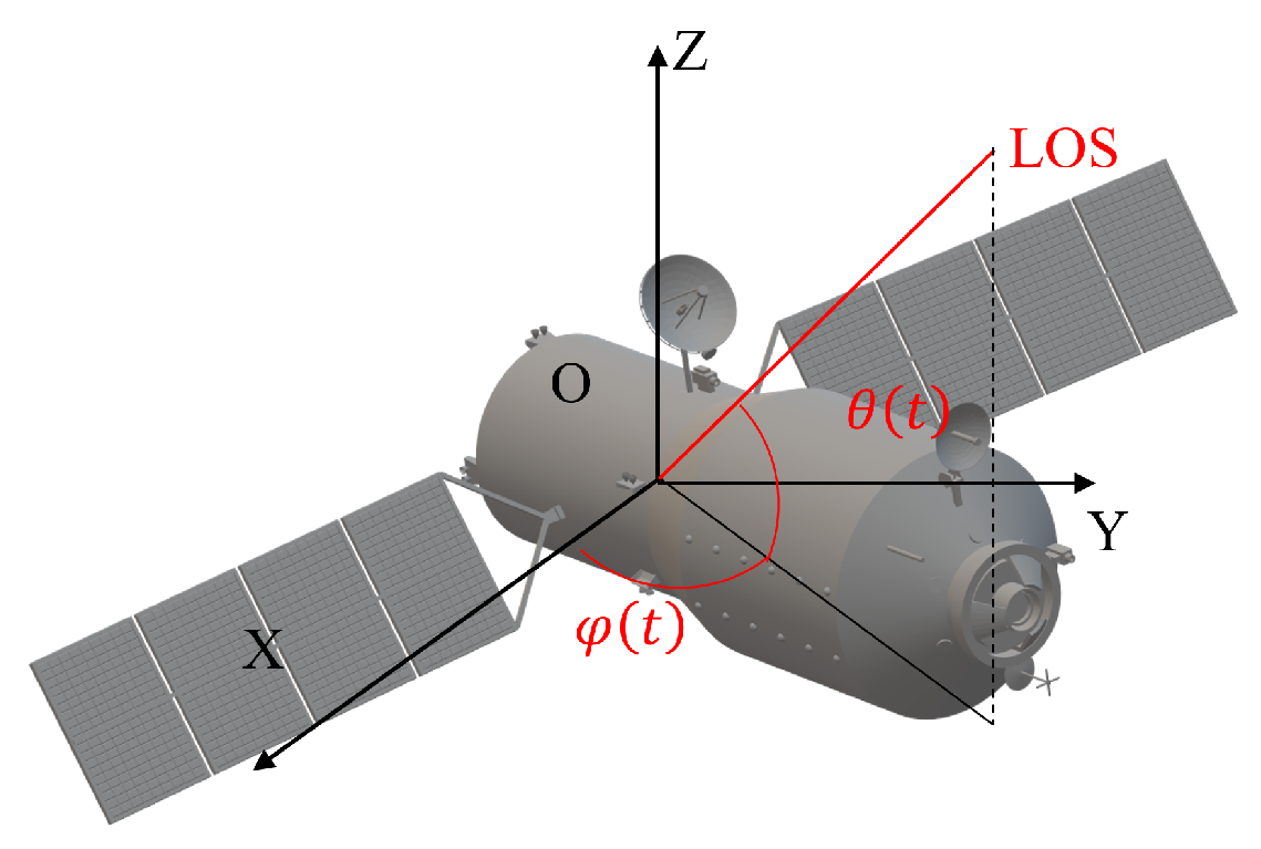
By locating both an optical sensor and an ISAR system in the same position, as shown in Figure 1, the two sensors simultaneously observe the on-orbit space target [32,33]. The vectors and denote the LOS of the optical and ISAR imaging moment, respectively. There is a difference in the definition of the imaging moment between these two sensors. Specifically, the snapshot time [27] and the central time of the coherent processing interval (CPI) [34] are used as the imaging moment for the optical sensor and ISAR system, respectively.
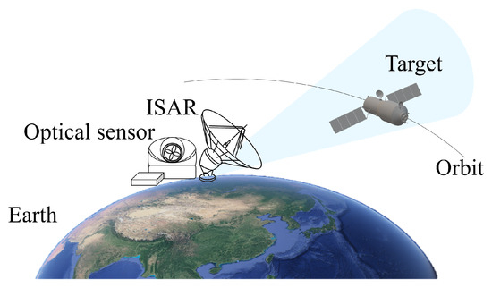
Figure 1.
The joint optical-and-inverse synthetic aperture radar co-location observation system.
Based on the constructed observation scenario, it can be seen that the two sensors share the same viewing LOS. The LOS vector is often defined in the measurement coordinate system (MCS). It is necessary to transform it to the orbital coordinate system (OCS) to simplify the subsequent derivation [35]. Assume that the transformed LOS is . The target and in the OCS are illustrated in Figure 2. The LOS is depicted as red lines, while is the elevation angle, and is the azimuth angle. Then, and can be defined as follows:
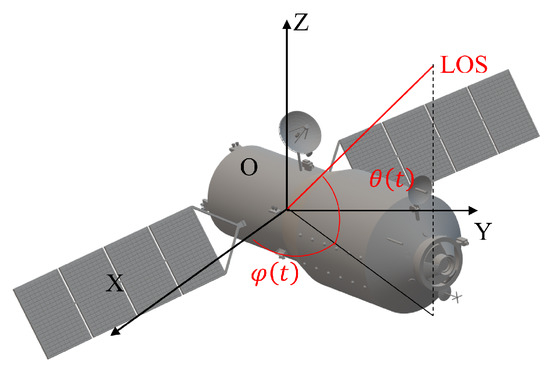
Figure 2.
The schematic of the line of sight.
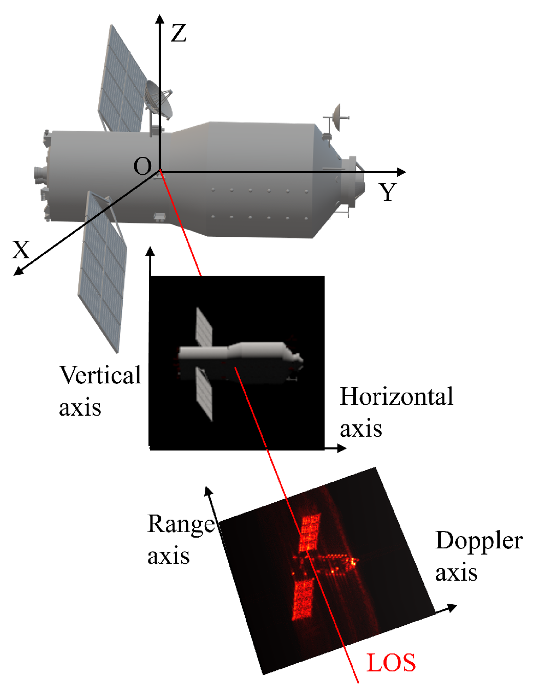
When the optical sensor and ISAR share the same LOS, an optical and ISAR image pair can be obtained at each observation time instant. Different pairs of images constitute an image set. The imaging projection relationship of each image pair is illustrated in Figure 3. As for the space target, optical imaging is based on diffuse reflection. Since space targets are usually far away, optical imaging can be considered orthogonal. Then, the horizontal axis and the vertical axis are perpendicular to the LOS simultaneously. The resolution units in horizontal and vertical directions, i.e., and , can be obtained in advance [1,36]. However, ISAR imaging is primarily based on the backscattering. The range axis is parallel to the LOS and perpendicular to the cross-range axis . In addition, is perpendicular to the equivalent rotation vector. Assume that C and B represent the speed and bandwidth of the signal. The range resolution unit can be solved as
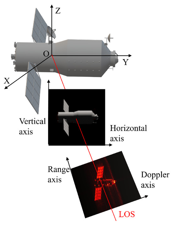
Figure 3.
The imaging projection relationship of each pair of inverse synthetic aperture radar and optical images.
For non-cooperative targets with slow rotation or unstable chaotic rotation, only the Doppler cell can be determined, while the cross-range resolution unit is difficult to obtain directly.
Assume that there is a point on the target located in the OCS. For the optical image plane, denotes the optical projection matrix, and the projection relation of this scattering point can be written as
where and denote the pixel position coordinates of projected along and , respectively.
For the ISAR imaging plane, denotes the ISAR projection matrix, and the projection relation of this scattering point can be described as
where and represent the pixel position coordinates of projected along and , respectively.
After constructing the joint optical-and-ISAR COS, simultaneous observations are made by the optical sensor and ISAR. Consequently, different optical and ISAR image pairs can be acquired, sharing the same observation time instant. In processing the optical image, a time synchronization method described in [27] is utilized, and the observation time is defined as the snaptime. As for the ISAR image, the observation time is defined as the central time of the CPI. Since the snaptime of the optical image is much shorter than the CPI of the ISAR image, the central instant of an ISAR image can be selected according to the optical images [28]. Furthermore, ISAR imaging algorithms are used to solve the defocusing phenomenon of the ISAR image caused by the complex target motion and large rotation angle observations [2,37,38]. After processing, multiple pairs of optical and ISAR images are acquired for space targets.
3. Methodology
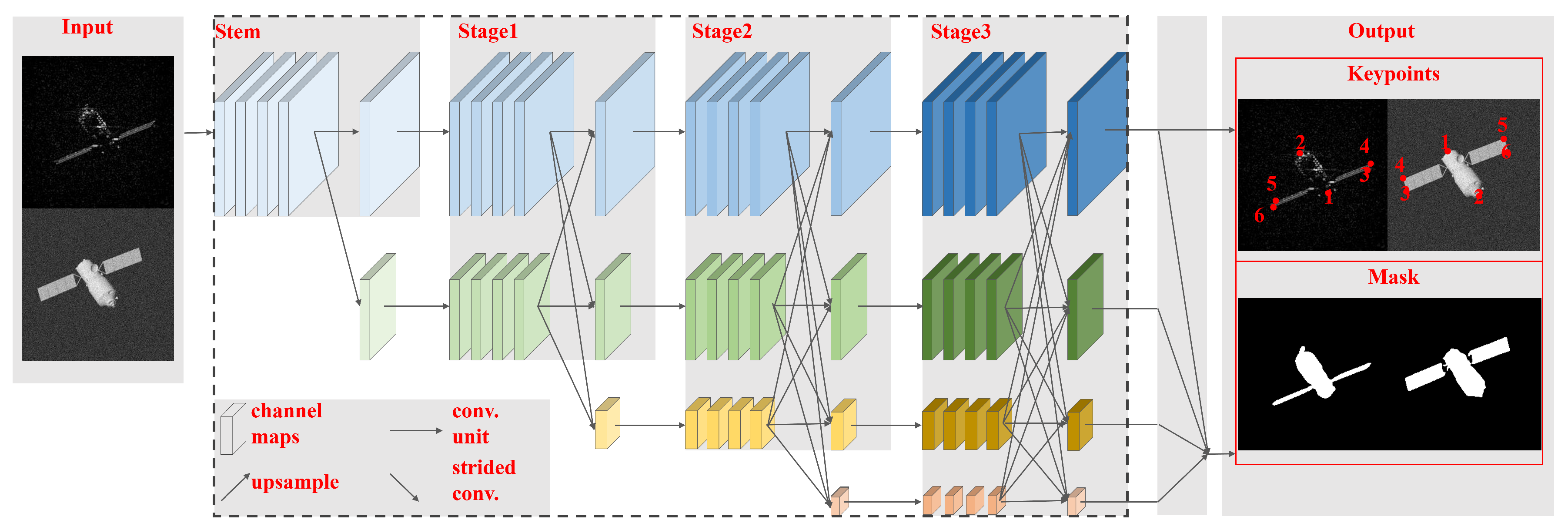
Based on the paired ISAR and optical images obtained in Section 2, four modules for 3-D reconstruction based on optical and ISAR images are proposed in this section. As shown in Figure 4, the key point and mask features of the image are initially extracted in Section 3.1 by using high-resolution net (HRNet). Subsequently, the image offsets between the optical and ISAR images in each pair are estimated and corrected in Section 3.2. Next, the rotational and positional offsets between adjacent pairs are derived, and the corresponding spatial offset correction method is proposed in Section 3.3. Finally, the 3-D voxel reconstruction is achieved by employing the VTM-GL method in Section 3.4. In Section 4, the proposed algorithm is summarized, with its structural representation depicted in Figure 4.
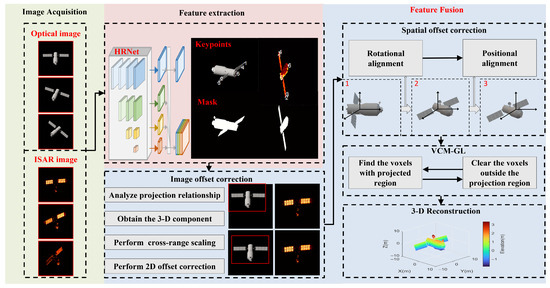
Figure 4.
3-D reconstruction module from optical-and-inverse synthetic aperture radar images.
3.1. Feature Extraction
As for the 2-D image, key points such as the corners of the solar panel and the main body can provide a precise projection geometry description of the space target. Meanwhile, the extracted mask can complement the missing parts of the target image caused by the occlusion of different components and the anisotropy of electromagnetic scattering characteristics. In terms of key points extraction and mask generation, extensive deep-learning-based methods have shown superior performance [39,40,41]. Considering that HRNet [41] can always achieve the superior performance in image representation, it is utilized for image key point extraction and mask generation.
HRNet adopts a cascaded pyramid network structure and maintains high-resolution image features throughout the entire process, ensuring that deep-level features are preserved. In addition, such an end-to-end high-resolution representation network is particularly suitable for processing optical and ISAR images of space targets characterized by small image sizes and subtle details in target parts. The network structure of HRNet is shown in Figure 5. Initially, the input image undergoes preliminary feature extraction. The downsampled results of the initial feature extraction and the original features are then separately input into different depth channels in Stage 1. In the subsequent three stages of the network, the final layer of each stage performs feature fusion across different depth layers. Subsequently, downsampling is applied to obtain the next depth channel, reducing the image size by half each time. It is worth noting that both high-resolution and low-resolution representations of features are processed simultaneously in this network. In Stage 3, the output of the network is divided into four resolution levels. The highest-resolution feature is directly output as the heatmap for key point prediction. By upsampling the features from the four resolution levels to the highest resolution, the mask can be obtained.
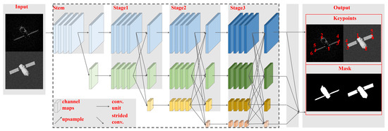
Figure 5.
The structure of the high-resolution net, where the red numbers are the numbers of the extracted key points.
As shown in Figure 5, the output of HRNet contains the target key points. Six key points of optical and ISAR images and can be obtained, respectively, and . Further, it can be solved for the projected lengths of the key components, i.e., the main body b, the long side , and the short side of the solar panel. The projected length r of the main body can be rewritten as
It is worth noting that the key points feature coordinates extracted from the aforementioned 2-D images are pixel values. The precise cross-range resolution cell of the ISAR image cannot be determined in advance. Therefore, the calibrated , , and are true values, while remains a pixel value. In turn, the projected length of and can be represented in a similar way. It is important to note that, in fact, our method only requires the extraction of four non-coplanar points to compute three sets of non-coplanar pointing features based on (5). This flexible key points extraction step ensures that the OC-V3R-OI method remains adaptable to targets with severely damaged or deformed structures.
3.2. Image Offset Correction
Due to the fact that optical and ISAR images originate from different sensors, the image alignment in each pair becomes crucial in 3-D reconstruction. Through the feature extraction using HRNet as described above, we can obtain key points and the projected lengths of the key components in both optical and ISAR images. These key points accurately describe the projected position information of the target in the 2-D images, thereby aiding in addressing the image alignment and resolving the spatial geometric projection relationships.
The main body is denoted as , while the long and short side of the solar panel are represented by and , respectively. Then, the space geometric projection relationship of the main body satisfies
where is the projection matrix. Under the joint optical and ISAR COS, the horizontal projection axis , vertical projection axis , and LOS vector are mutually perpendicular. Then, the is a full-rank matrix. Hence, the 3-D spatial direction of the main body can be represented as
Similarly, and can be estimated as
and
Indeed, , , and represent the attitude of the target at the current moment.
Furthermore, the projections of the above three 3-D key components on the Doppler axis are the Doppler axis projection lengths extracted in the previous section, and this projection relation can be described as
If the above selected components are not in the same plane, then the calibrated Doppler projection axis can be determined as
Hence, the Doppler resolution cell and the Doppler projection axis can be estimated by
and
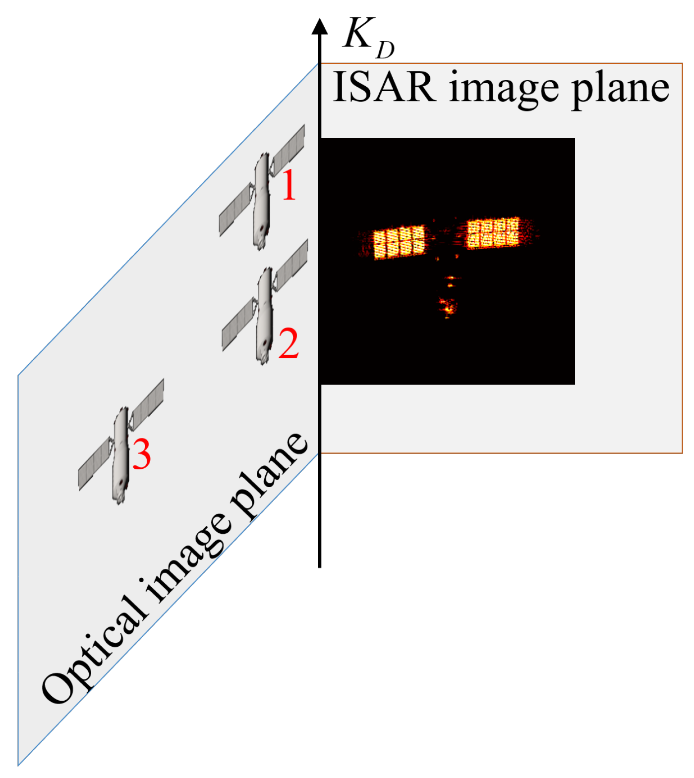
The projection relations for a space target with offsets on the optical and ISAR images are depicted in Figure 6. Square 1 represents the optical projection of the space target, while square 3 represents the ISAR projection position of the target. Since , , and are perpendicular to each other, and is coplanar with the optical plane consisting of and , a common reference is shared on the optical and ISAR images. It is evident from Figure 6 that center positions of the above two square projections do not coincide in the same Doppler axis direction. This is the essential cause of the offset in a pair of images. Then, by shifting the optical image mask and key point coordinates along the Doppler direction according to the projection difference, the offset can be corrected. Fortunately, and can form a rectangular coordinate system due to the fact that they are perpendicular. Therefore, the Doppler axis can be expressed as

Figure 6.
The schematic of image offset correction between optical-and-inverse synthetic aperture radar images.
Actually, Equation (14) can be transformed into the matrix form as
The coefficients a and b can be solved as
Assume that the th key point is from the optical image. Then, the projection of this point on can be computed as
Further, extracting of the point from the ISAR image and solving for the deviations of and can be computed as
As shown in Figure 6, optical image 1 is shifted along the Doppler axis in the positive direction, which is equivalent to shifting along and along in the positive direction. Optical image 1 is corrected to optical image 2, and the image offset correction is resolved.
Further, the accuracy requirements for image offset are analyzed. In the OC-V3R-OI method, image offset affects the mask features, which in turn impacts the mismatch in the projection space, ultimately influencing the 3-D reconstruction results. The image mask represents the projected area of the target on optical and ISAR images. The projection region is mapped onto a spatial cylinder along the normal direction, and the intersection space of the spatial cylinders corresponding to each imaging plane represents the actual occupied space of the target. When there is an offset in the image mask, the spatial intersection decreases, leading to a reduction in the completeness of the target reconstruction.
In real-world scenes, the distribution of space target features is non-uniform, making quantitative analysis difficult. Therefore, we assume a uniform distribution of space target features. Using the long edge of Tiangong-1’s solar panel as a reference, we define a sphere with a diameter of 20 m. The projection of this sphere on the image is always a circle. If the image offset error per frame is a certain number of pixels and the sphere is observed from all angles, the following equation can be derived to ensure that the spatial intersection occupies 80% of the actual space:
Solving the inequality above gives m. Thus, on average, the image offset error must be kept below 0.7182 m to meet the accuracy requirements for 3-D reconstruction.
3.3. Spatial Offset Correction
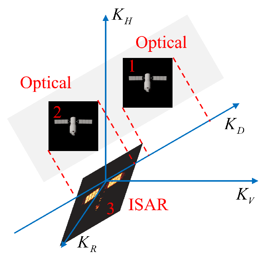
In Figure 7, the 3-D spatial position offset is explained. It can be seen that target 1 and target 2 have different projection components on the Doppler axis , which can be resolved by image offset correction. Then, target 2 and the target on the ISAR plane exhibit the same projection component on the Doppler axis. It is noteworthy that target 3 and target 2 will also share the same projection component on the Doppler axis . Although this offset does not affect the optical and ISAR projection relationship with a single pair, it will cause a misalignment in the 3-D space. Therefore, spatial offset correction is necessary.

Figure 7.
The schematic of three-dimensional spatial offset formation causes, where the red numbers are the numbers of the targets.
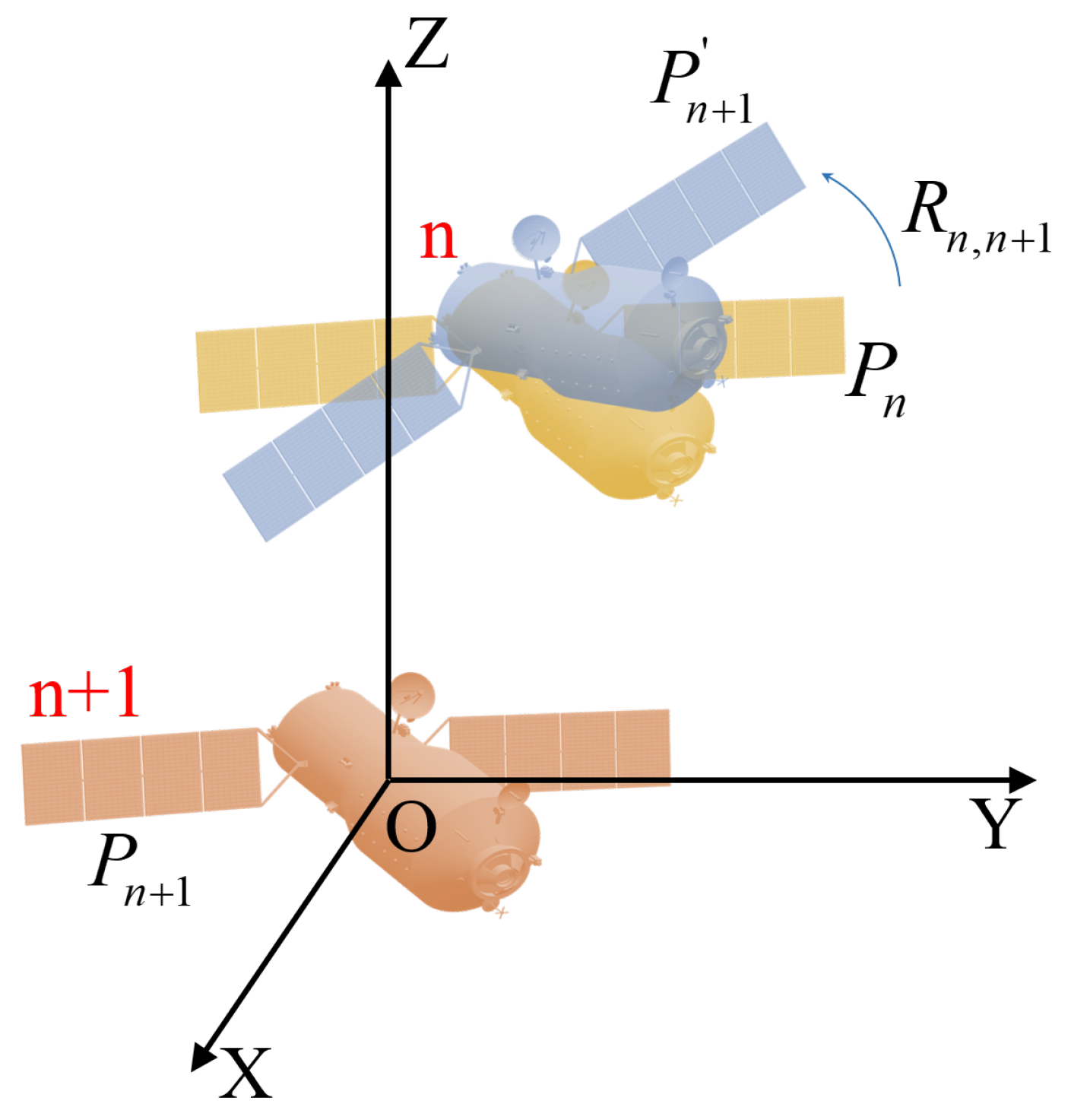
As depicted in Figure 8, the yellow target and the brown target represent the position and attitude of the target in the th and th frames. It can be seen that the blue target shares the same position as , but its attitude matches that of . Therefore, the spatial alignment from to can be decomposed into rotational and positional alignment. The points can be corrected to through spatial rotation, and then moved to through spatial translation to achieve spatial offset correction. The rotational alignment is firstly derived. Let the 3-D direction vectors of typical components be denoted by , , and in the th pair of images. Then, the rotation matrix correcting the space target attitude between the nth pair of images and the th pair of images can be expressed as
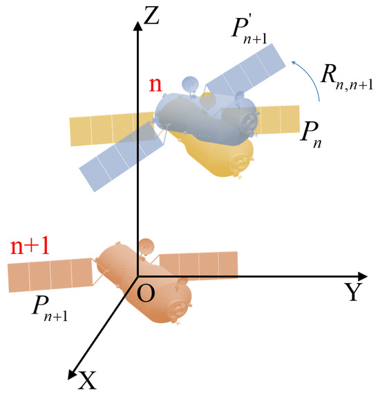
Figure 8.
The schematic of spatial offset correction of the attitude at the th moment and the attitude at the th moment.
Therefore, for adjacent pairs can be solved as
Further, the projection relation of the th key point at the th frame on the optical-and-ISAR image can be described as
Then, the 3-D point can be solved as follows:
According to the rotation relation (20), the target at the th observation time can be transformed to the same attitude as the space target at the th observation time. The expression is presented as
After the rotation correction, and only remain as positional displacement in 3-D space. The translational offsets in the three axes of 3-D space can be solved as
By shifting the according to the , the translational offsets can be corrected, and the spatial alignment is completed.
3.4. Voxel Trimming Mechanism Based on Growth Learning
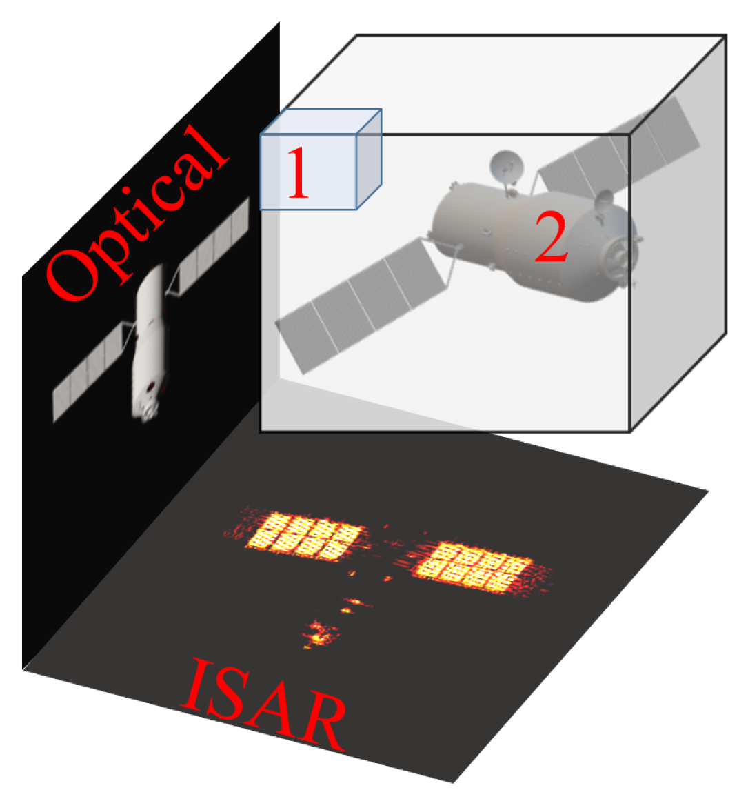
The processing of image alignment and the establishment of projection geometry relations provide accurate and sufficient information for 3-D reconstruction. According to the projection relation, the viewpoint relation from 3-D space to 2-D image can be established explicitly. Based on the mask extraction results during feature extraction, the range of the target on the image can be complemented and normalized. Thus, 3-D geometry reconstruction can be achieved by voxel trimming processing. As shown in Figure 9, voxel 1 and voxel 2 are projected onto two separate images, respectively. Voxel 2 is regarded as true since it is projected within both the ISAR and optical mask regions. However, voxel 1 projects outside the optical or ISAR mask region and is therefore considered to be a spurious voxel and should be removed.
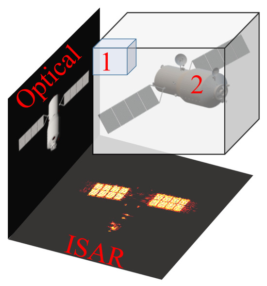
Figure 9.
The projection relationship of a voxel to the optical and inverse synthetic aperture radar imaging plane.
To increase the robustness of voxel trimming processing, a voxel trimming mechanism based on growth learning (VTM-GL) is designed. Assume that N image pairs are available for 3-D geometry reconstruction. VTM-GL divides the learning period into three stages. First is the early stage, which spans from the first pair to the th pair, and is usually set to be . Next, the middle stage spans from the th pair to the th pair, and is usually set to be . The final stage is from the th pair to the Nth pair.
The VTM-GL method requires accumulated experience in the early stage. If a voxel is not within the extracted mask area, it will not be immediately trimmed. VTM-GL will accumulate the number of times q that each voxel is projected outside the mask area by . This allows VTM-GL to have a buffer period for accumulating learning in the early stage. In the middle stage, the method both relies on the experience gained during the early stage and continues to learn the number of times each voxel is outside the mask area, denoted as q. Simultaneously, it begins to trust the learned experience and clear voxels where . In the late stage, the VTM-GL has acquired sufficient experience. Continuous trimming may introduce unexpected errors. Therefore, learning slows down in the late stage, and the trimming mechanism is paused. The OC-V3R-OI method ingeniously incorporates a rebound mechanism while learning q. When a voxel is projected within the mask area, an additional adjustment is applied with . Finally, after the late stage, voxels with are trimmed again. This method achieves a well-designed voxel trimming mechanism, consisting of an early stage of accumulation learning, a middle stage of rapid learning, and a late stage of slow learning.
4. Algorithm Summation and Computation Complexity Analysis
This section is based on the various steps of the 3-D reconstruction methodology described above. In our reconstruction process, there are four key steps: feature extraction, image offset correction, spatial offset correction, and the VTM-GL mechanism. Firstly, feature extraction employs advanced methods to extract mask and key point features from the input optical and ISAR images, which serve as the foundation for subsequent offset corrections and the VTM-GL process. Secondly, the key point features are used to solve the offset relationship between images and the projection relationship between the 3-D space and the 2-D images. Next, starting from the second frame, we compute the rotational offset and translational offset, and rotate the voxel from the previous frame to align with the current frame’s spatial configuration, ensuring consistency between consecutive frames. Finally, based on the projection relationship, the corrected image offsets, and the spatially consistent voxels, we use the VTM-GL mechanism to achieve the 3-D reconstruction of the voxels. Specifically, the procedure is summarized as Algorithm 1.
| Algorithm 1: The process of three-dimensional reconstruction. |
|
Due to the design of voxel-related processing, it is necessary to analyze the time complexity of the algorithm. The time complexity of the OC-V3R-OI method is mainly influenced by four factors: the number of image pairs N, the height H and width W of the images, and the number of voxels M. Firstly, each of the M voxels needs to be initialized individually, so this process has a time complexity of . Then, the main computational work occurs within a loop that iterates over N image pairs. Each iteration involves several steps. Step 4 involves matrix inversion and multiplication, so the time complexity is constant . The complexity for step 5 is , as it needs to process every pixel in the image. Like step 4, this involves matrix inversion and multiplication, so step 7 also has a time complexity of . Step 8 requires a loop over all M voxels, so the time complexity is . The final step, step 9, involves checking each voxel, leading to a time complexity of . Summing the time complexities of all these steps, the overall time complexity of an iteration can be solved as
Since this process is repeated for N pairs of images, the total time complexity for the entire method is calculated as
5. Experiments
To validate the effectiveness of the OC-V3R-OI method, we designed and conducted a series of experiments, which are organized into three main sections. In Section 5.1, we provide an overview of the data required for the experiments. In Section 5.2, we outline the metrics used to assess the performance in the experiments. In Section 5.3, we conduct an evaluation of the method’s effectiveness, performance, and comparison with other traditional methods based on the aforementioned data and evaluation metrics.
5.1. Data Description
The OC-V3R-OI method is established on the joint optical-and-ISAR COS. Therefore, a simulation scenario is constructed to validate the OC-V3R-OI method. Firstly, a typical target of Tiangong-1, as shown in Figure 10, is selected, and then a model corresponding to the key points and mask database is constructed. HRNet is trained to obtain the key point features and mask features of the ISAR and optical images [41]. For ISAR images, they are generated from the X-band, and B is set to 1.5 GHz. Then, we generate the full-angle electromagnetic simulation data of Tiangong-1 using the physical optics (PO) algorithm [42,43], and the SNRs (signal-to-noise ratios) of ISAR images are distributed from 0 dB to 30 dB. Subsequently, 35,000 ISAR images are generated. For optical images, the image SNRs are distributed from 0 dB to 30 dB, and the horizontal and vertical resolution units are set to 0.1 m. The ray-tracing method is then used to generate 7700 full-angle optical images [44,45].
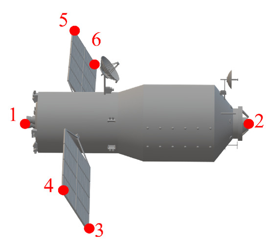
Figure 10.
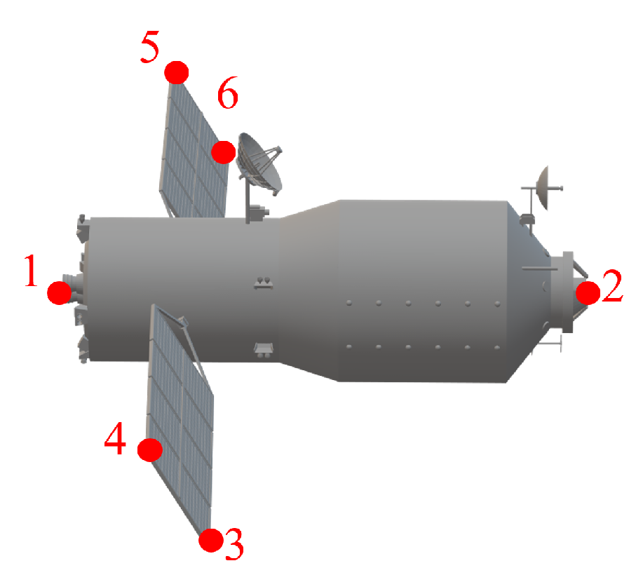
Three-dimensional model of Tiangong-1 and the six marked key points, where the red numbers are the numbers of the extracted key points.
As is well known, the edge point information of the space target is relative robust and can be obtained through sustainable observation. Therefore, as shown in Figure 10, six non-coplanar structural edge points of the Tiangong-1 target are selected as key points, which are marked by red numbers 1 to 6. Consequently, the key points and masks on the 2-D images can be directly obtained through the projection of 3-D key points and target models. This allows for the rapid construction of the key point and mask database. Considering the significant differences between optical and ISAR image features, key point extraction HRNet and mask segmentation HRNet are trained separately for each type of image.
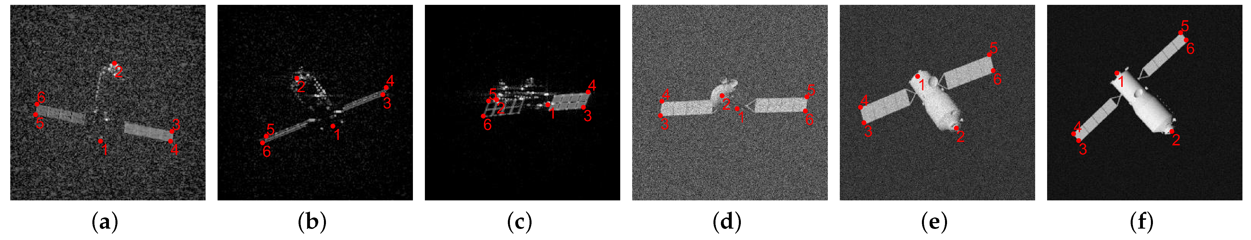
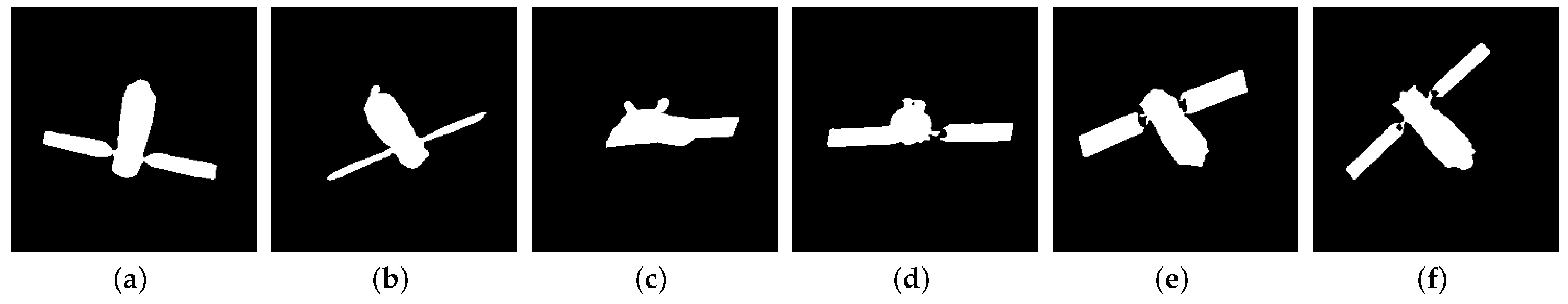
In contrast to the construction of the feature extraction network dataset, each optical and ISAR image pair needs to share the same viewpoint LOS since the scenes of the OC-V3R-OI method are built on optical-and-ISAR COS. We conduct five consecutive observations of the space target at five different elevation angles, with the target in different attitudes for each observation. In each observation LOS, the azimuth angle is distributed from 0° to 360°, with 100 evenly spaced LOS used as imaging moments. At each azimuth angle of the LOS, optical and ISAR image pairs are generated, with ISAR signal parameters and optical image resolution parameters consistent with those mentioned earlier. In Figure 11, partial optical and ISAR images generated for this experiment are shown, together with the extracted key points, and Figure 12 illustrates the extracted mask features. It is evident that the superior feature extraction capability of deep learning methods provides a solid data foundation for 3-D reconstruction.
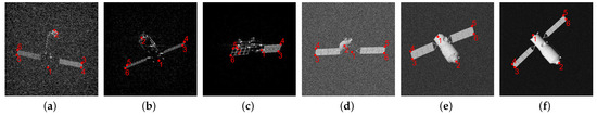
Figure 11.
Extraction results of six key points on two-dimensional images, where the red numbers are the numbers of the extracted key points: (a–c) inverse synthetic aperture radar images; (d–f) optical images.

Figure 12.
Extraction results of masks on two-dimensional images: (a–c) inverse synthetic aperture radar images; (d–f) optical images.
5.2. Performance Evaluation Metrics
To better evaluate the performance of the OC-V3R-OI method, several indicators were selected for quantitative analysis. The model intersection over union (MIoU), Chamfer distance (CD), number of points, and attitude estimation error are used to respectively evaluate the structural refinement, structural similarity, structural density, and attitude accuracy of the reconstruction result.
Inspired by the concepts of accuracy and integrity in [25], the MIou metric is devised to assess the similarity of reconstructed refinement. Following the definition in [25], the effective grid count , the reconstructed grid count , and the true grid count can be obtained. Therefore, MIou can be defined as
The CD is a crucial metric for assessing the structural similarity between the real target model and reconstruction result. CD has been widely employed in objective functions and evaluation criteria for 3-D reconstruction tasks [46]. Assume that and represent the reconstruction result and the ground truth target model, respectively. CD can be described as
where x and y denote the coordinates of points in and , respectively. If this distance is larger, it indicates a greater difference between the two models. Conversely, if this distance is smaller, it suggests that and are more similar.
The number of points directly corresponds to the number of reconstructed voxels, serving to evaluate the structural density of the reconstruction results.
The angle error can evaluate the attitude estimation accuracy. First, the angle between the estimated 3-D component direction and the true component direction is calculated at each observation. Then, the average angle of N frames of observation is computed as the angular error. The angle error can be calculated as
5.3. Analyses
In this section, we conduct comprehensive analyses of the proposed method through effectiveness analysis, performance analysis, and comparison analysis. Specifically, Section 5.3.1 evaluates the effectiveness of the OC-V3R-OI method. Section 5.3.2 assesses the performance of the method, testing its robustness. Section 5.3.3 compares the OC-V3R-OI method with existing methods to highlight its superiority.
5.3.1. Effectiveness Analysis
The OC-V3R-OI method is independent of the motion type of the target, making it applicable to a space target with arbitrary motion. For the generated five-circle images mentioned above, the target model is triaxially stabilized in the orbital coordinate system during a single circle observation, while a random attitude difference exists between any two circles. Therefore, when combining data from multiple circles, the attitude exhibits irregular variation. Thus, multi-circle data are selected, in which case the space target can be considered to be in a chaotic motion model.
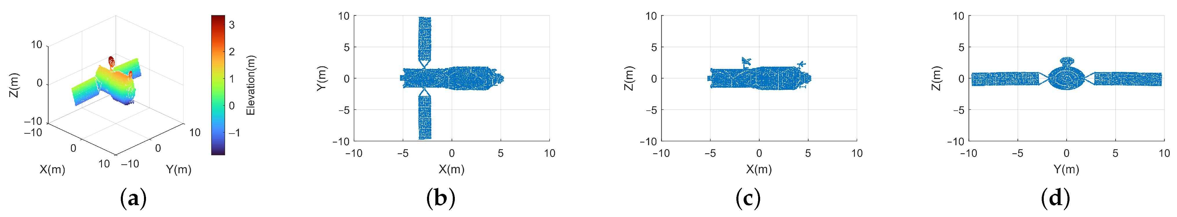
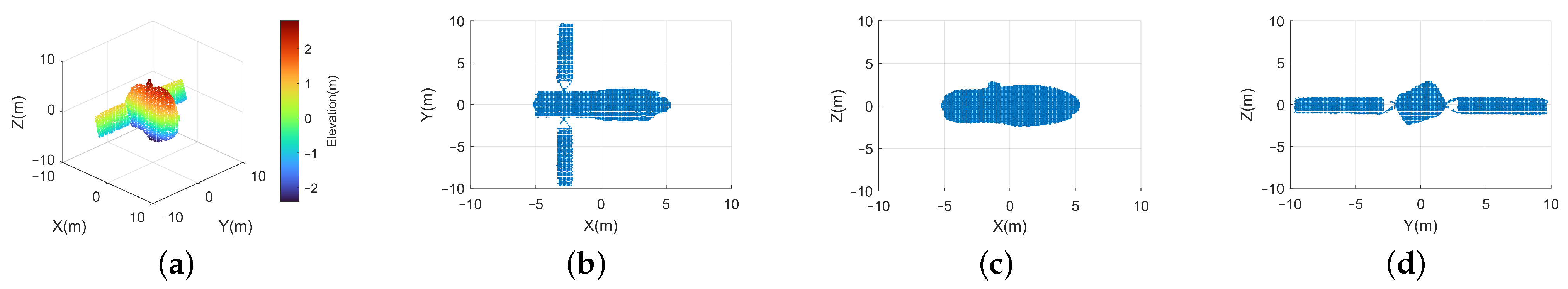
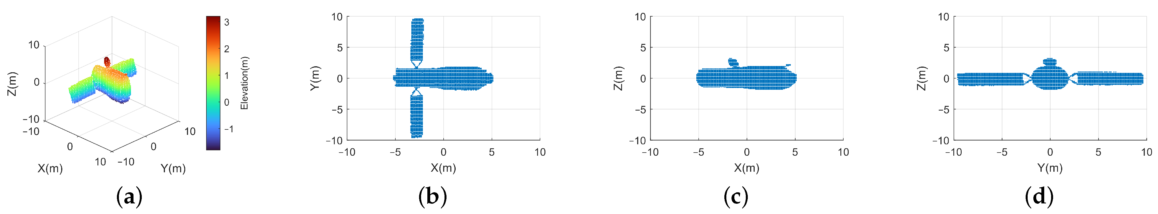
To validate the effectiveness, the signal parameters and scene are consistent with the above description, and the image SNR is set to 30 dB. Firstly, 50 pairs of images from the first observation circle are randomly selected, with the target being a triaxially stabilized target. The OC-V3R-OI method is executed after extracting key point features and mask features using HRNet. The real target model is shown in Figure 13, which illustrates the real 3-D model and its three views. The reconstruction results are shown in Figure 14. Then, for the target with chaotic motion, 10 pairs of images are randomly selected from each circle to form a set of 50 pairs of images, which are used to verify the effectiveness for chaotic motion targets. Figure 15 shows the reconstruction results. It can be observed that the 3-D geometry of both single-circle observations of the triaxially stabilized target and multi-circle observations of the chaotic motion target can be reconstructed successfully. Additionally, the critical components such as the main body and solar panel can be robustly reconstructed. Particularly, the 3-D reconstruction results for the chaotic motion target across multiple observation cycles benefit from their diverse perspectives, resulting in superior reconstruction performance for the component details of the space target.

Figure 13.
Real model of Tiangong-1: (a) oblique view; (b) projected on the O-XY plane; (c) projected on the O-XZ plane; (d) projected on the O-YZ plane.

Figure 14.
Reconstructed model for triaxially stabilized target of the single-circle observations: (a) oblique view; (b) projected on the O-XY plane; (c) projected on the O-XZ plane; (d) projected on the O-YZ plane.
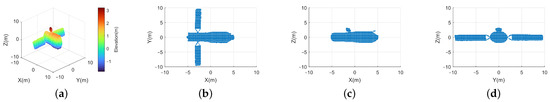
Figure 15.
Reconstructed model for chaotic motion target of the multi-circle observations: (a) oblique view; (b) projected on the O-XY plane; (c) projected on the O-XZ plane; (d) projected on the O-YZ plane.
Furthermore, the four indicators mentioned earlier were selected to quantitatively analyze the performance. As shown in Table 1, the results of the relevant indicators are recorded. The MIoU, CD, number of points, and attitude estimation error of the 3-D reconstruction result under single-circle observation are 88.83%, 0.1180 m, 107127, and 0.7555°, respectively. The corresponding values are 91.85%, 0.0848 m, 107644, and 0.7213° under multi-circle observations. This further validates the OC-V3R-OI method’s capability to extract 3-D information from targets with chaotic motion. The reconstruction results of the space target with triaxially stabilized motion or chaotic motion demonstrate good refinement, similarity, density, and attitude estimation capabilities.

Table 1.
The evaluation values of the reconstructed geometries.
5.3.2. Performance Analysis
The robustness will be verified using the four aforementioned metrics. The same image data and scene parameters as in Section 5.1 are utilized to conduct this analysis, and the target motion type is chaotic motion. In particular, the impact of different input types on the performance will be analyzed. This analysis will facilitate the identification of the contribution of each input to the results, thereby enabling a more comprehensive assessment of the performance of the method in diverse scenarios. As shown in Algorithm 1, the input data consist of multiple sets of target mask features and key point features, horizontal and vertical axes, range axis, and resolution units for ISAR and optical images. It is assumed that the parameters of the three projection axes are precisely known due to the fact that this information can be obtained from the observation process of the optical sensor and ISAR system. The projection axes and their calibrated resolution units can be precisely acquired. Variations in masks, key points, and the number of image pairs will have different impacts on the performance of the 3-D reconstruction results.
Specifically, the mask features represent the distribution of the target in the 2-D image. Errors in the mask features directly impact the voxel projection stage in the VTM-GL step. These errors may cause the learning factor q of voxels that should not be projected into the mask area to increase, or the q of voxels that should be projected to decrease. These changes directly degrade reconstruction performance, negatively affecting metrics such as MIoU, CD, and the number of points.
Key point features determine the absolute position of target features. Errors in these inputs primarily affect the 3-D orientation of components during image offset correction, including the target attitude, which subsequently disrupts the solution of the Doppler axis. This ultimately introduces errors in image offset, causing misalignment between the ISAR and optical images in 3-D space. Moreover, key points dictate the spatial rotation and offset relationships. These cumulative errors lead to mismatches in 3-D space, directly impacting reconstruction performance and degrading metrics such as MIoU, CD, angle error, and number of points.
The number of images determines the amount of information available for 3-D reconstruction. When the image count is high, more target information can be incorporated, but errors may also accumulate, leading to a reduction in the voxel count. Conversely, with fewer images, while errors are relatively smaller, insufficient information may result in higher voxel counts. The OC-V3R-OI method mitigates error accumulation when more images are used by leveraging VTM-GL, effectively utilizing image information. Consequently, metrics such as MIoU and CD improve, and as voxel refinement progresses, the voxel count decreases before stabilizing.
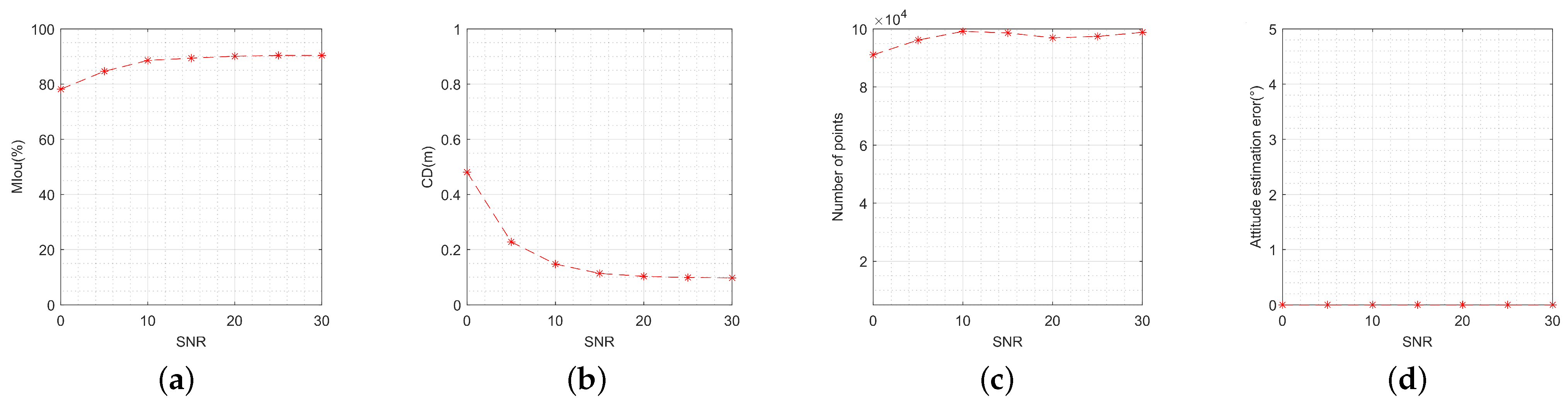
To analyze the impact of different mask extraction features, we fix the input to 50 pairs of images, with the key point features being the real ones. It is worth noting that HRNet, which has been trained earlier, produces masks with different intersection over union (Iou) values under varying SNRs. This allows us to simulate the impact of different mask extraction features by using HRNet to extract images with varying SNRs. The SNR varies from 0 dB to 30 dB. The step size was set to 5 dB, and 100 Monte Carlo experiments were performed at each SNR level. Figure 16a–c show the MIou, CD, and number of points for the reconstruction results. Evidently, when the SNR is greater than 10 dB, these metrics are all above 85%, 0.2 m, and 90,000 points, respectively, which are generally acceptable for most 3-D reconstruction tasks. In addition, as shown in Figure 16c, the increased SNR allows some of the false points to be cleared, resulting in a reduction in the number of points around 20 dB. It is evident from Figure 16d that the attitude estimation error is approximately unchanged and is almost unaffected by masks.
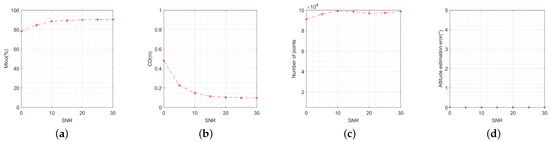
Figure 16.
Performance metrics’ variation with signal-to-noise ratio: (a) variation of model intersection over union; (b) variation of Chamfer distance; (c) variation of number of points; (d) variation of attitude estimation error.
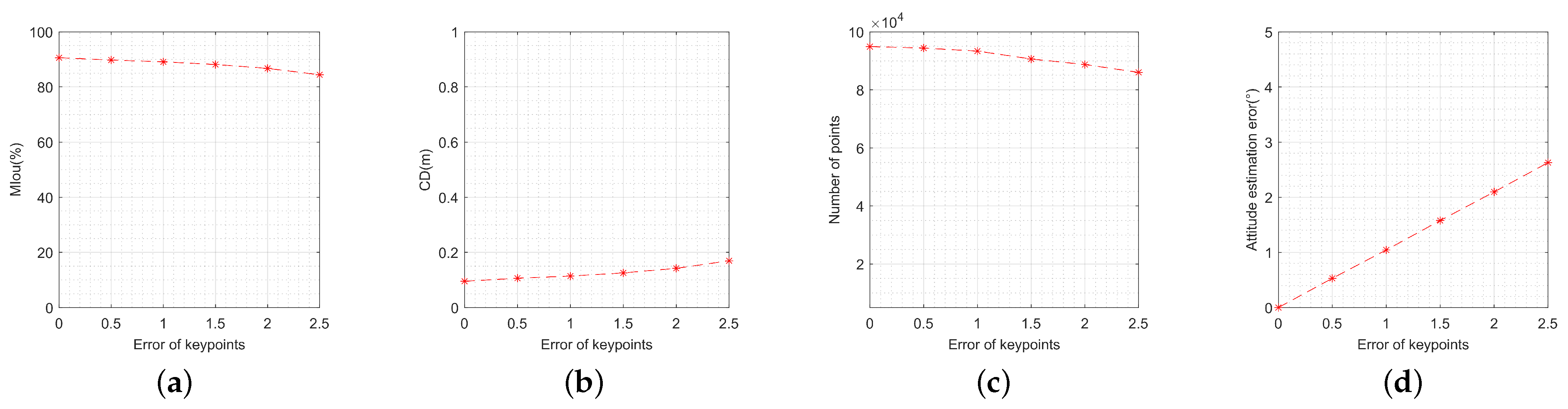
To analyze the performance under different key point extraction errors, 50 pairs of images are used as input. The image SNR is fixed at 30 dB. Random position errors are added to the original key point features, with the standard deviation of the position error ranging from 0 pixels to 2.5 pixels. The step size was set to 0.5 pixels and 100 Monte Carlo experiments were performed at each value. Figure 17 displays the MIou, CD, number of points, and attitude estimation error of the 3-D reconstruction results. It can be observed that these metrics are all above 80%, 0.2 m, 80,000 points, and 3°, respectively, which are generally acceptable for most 3-D reconstruction tasks. The attitude estimation error is linearly correlated with the key point features, as shown in Figure 17, indicating the attitude estimation error increases with the key points error gradually.
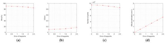
Figure 17.
Performance metrics’ variation with the error of key points: (a) variation of model intersection over union; (b) variation of Chamfer distance; (c) variation of number of points; (d) variation of attitude estimation error.
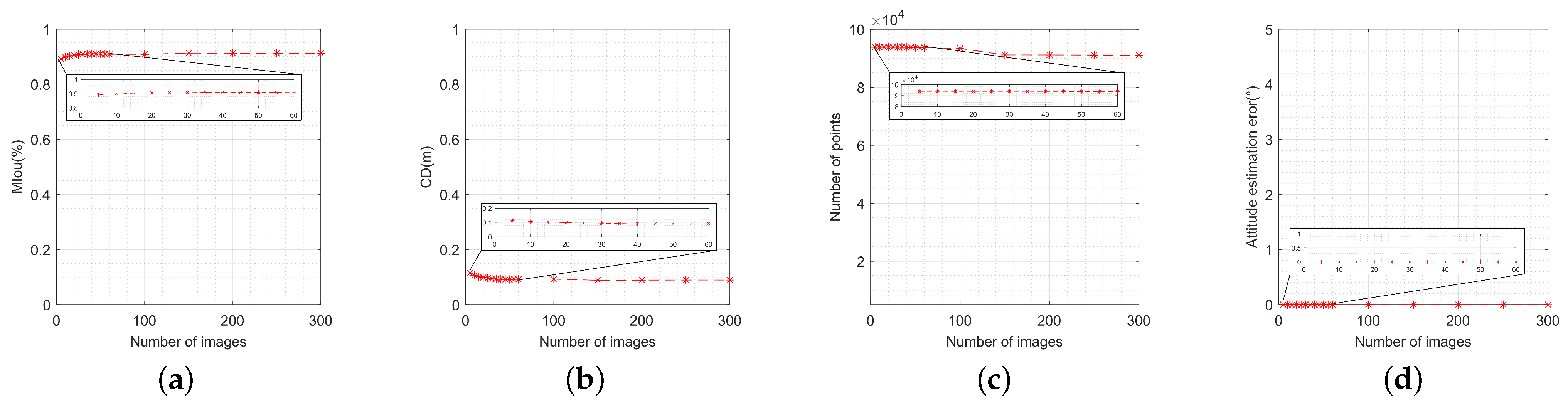
To analyze the performance under both small and large image pair numbers, the image SNR is fixed at 30 dB, and the original key points are used. Firstly, the input image pair number varies from 5 to 60 uniformly with a small step size of 5, and varies from 100 to 300 uniformly with a larger step size of 50. The reconstruction performance is then analyzed in terms of its variation with the number of images. Figure 18 illustrates MIou, CD, number of points, and attitude estimation error. It can be observed that the metrics for MIou, CD, and number of points are all above 85.0%, 0.15 m, and 90,000 points, respectively, which are generally acceptable for most 3-D reconstruction tasks. These three metrics also converge at an image number of 150 pairs. Meanwhile, Figure 18d also shows that the attitude estimation error is hardly affected by the image pair number. Hence, the attitude estimation error is approximately unchanged under different image pair numbers. Moreover, even with a larger number of image pairs, this method maintains high performance and will not continuously accumulate error, validating the robustness of the VTM-GL method.
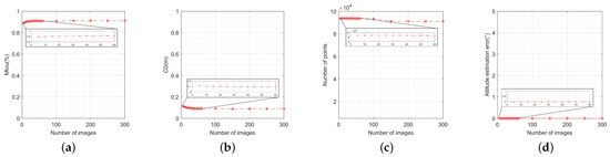
Figure 18.
Performance metrics’ variation with the number of images: (a) variation of model intersection over union; (b) variation of Chamfer distance; (c) variation of number of points; (d) variation of attitude estimation error.
It is noteworthy that the attitude estimation errors in Figure 16d and Figure 18d are nearly zero. This outcome is determined by the specific attitude calculation method. According to (30), it can be seen that the attitude estimation error is determined by the pointing error of the key components, which is calculated using (7), (8), and (9). These errors, in turn, depend solely on the projection matrix and the extracted key points. Since Figure 16d and Figure 18d are designed to evaluate the variation of the attitude estimation errors with the SNR and the number of images, respectively, both the projection matrix and the key points are assumed to be accurate, which results in near-zero attitude estimation errors.
5.3.3. Comparison Analysis
In this section, different methods are selected for verifying the performance. For convenience, we refer to the OC-V3R-OI method without alignment and VTM-GL as the unaligned method and the clear method, respectively. We compare the OC-V3R-OI method with the EFF method [25], the unaligned method, and the clear method, using the same data and scene as in the previous sections. All four methods use the same key points and mask features. Since the EFF method lacks attitude information, and the accuracy of the reconstructed attitude for the unaligned method and the clear method is only related to key point extraction, we do not elaborate on the attitude accuracy indicator in this section.
In this experiment, we use five-circle observation data from Section 5.1. In real-world scenarios, space targets typically operate in a three-axis stabilized manner during the acquisition of single-orbit data, while their attitude may vary across different orbit passes. Consequently, multi-circle data provide greater diversity in observation angles, increasing the complexity of the observational scene. By randomly selecting images from these five-circle data, we introduce the uncertainties and variabilities inherent in real-world conditions, thereby enhancing alignment with actual operational environments and more accurately reflecting the performance of different methods. Additionally, the images are generated using highly realistic electromagnetic computation methods, ensuring that the scattering characteristics of the generated images are fundamentally consistent with those of real images. This guarantees their consistency with real-world scene images.
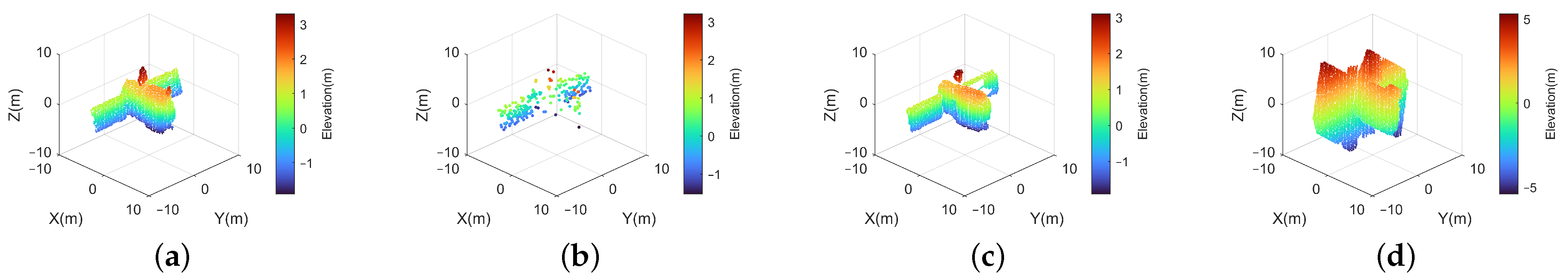
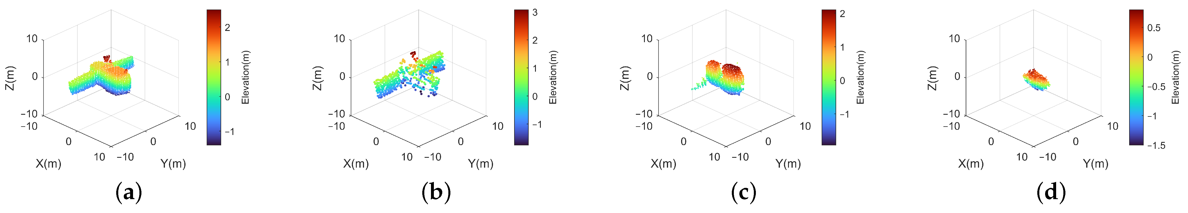
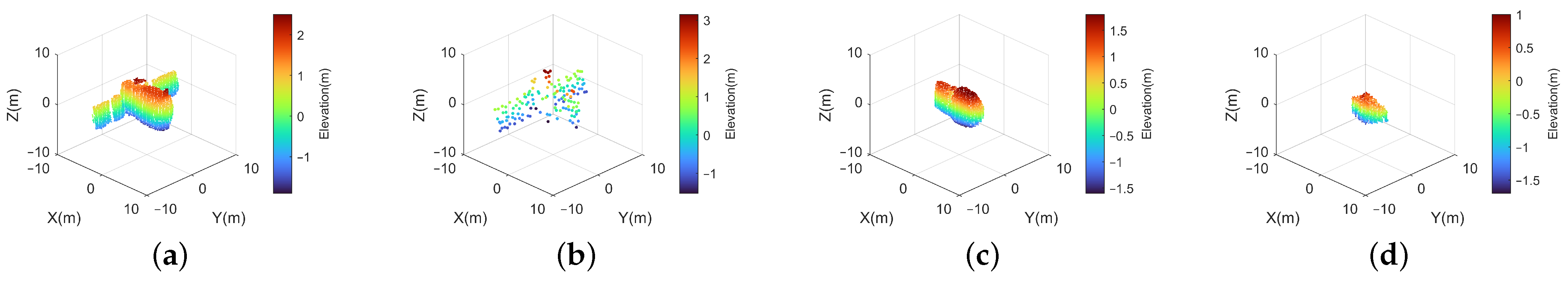
Assuming the number of image pairs is n, the key point error is , and the SNR is , the results for each parameter are shown in Figure 19, Figure 20, Figure 21 and Figure 22. It is evident that the results exhibit significant differences.
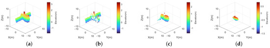
Figure 19.
Reconstruction results with : (a) the OC-V3R-OI method; (b) the EFF method [25]; (c) the clear method; (d) the unaligned method.

Figure 20.
Reconstruction results with : (a) the OC-V3R-OI method; (b) the EFF method [25]; (c) the clear method; (d) the unaligned method.
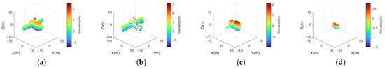
Figure 21.
Reconstruction results with : (a) the OC-V3R-OI method; (b) the EFF method [25]; (c) the clear method; (d) the unaligned method.
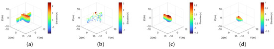
Figure 22.
Reconstruction results with : (a) the OC-V3R-OI method; (b) the EFF method [25]; (c) the clear method; (d) the unaligned method.
As shown in Figure 19 with and , both the OC-V3R-OI method and the EFF method achieve good results. Nevertheless, the clear method can only reconstruct the main body, with almost all solar panels being missing. The unaligned method fails to reconstruct.
As shown in Figure 20 with and , the OC-V3R-OI method can still obtain the precise 3-D structure, as it utilizes the rich information of fewer images in the chaotic motion state. The EFF method’s results are relatively sparse, with significant detail loss. The clear method can reconstruct the general components of the model, but with fewer details due to the smaller cumulative pair count. The unaligned method remains ineffective for reconstruction.
As shown in Figure 21 with and , both the OC-V3R-OI method and the EFF method are effective, reconstructing complete components with dense results. The clear method can only reconstruct the main body part, with almost all solar panels being missing. The unaligned method is ineffective for reconstruction.
As shown in Figure 22 with and , the OC-V3R-OI method, benefiting from the direct use of extracted mask features through the deep learning networks, is less affected by the image noise. In contrast, the EFF method, using original image input data, is severely affected by image noise, resulting in sparse reconstruction points and insufficient detail of the target description. The clear method can only reconstruct the main body, while the unaligned method remains ineffective. Clearly, the OC-V3R-OI method achieved the best performance.
Overall, the EFF method is applicable to chaotic motion targets. Instead, the performance of the EFF method relies on the utilized image number and image SNR. A large image number can provide a precise projection vector estimation result, which is the basis of the EFF method. Meanwhile, the reconstructed outcomes tend to be relatively sparse, leading to insufficient representation of the space target and resulting in the loss of structural details. Conversely, the unaligned method, lacking the correction of offsets in heterogeneous image sources and spatial displacement, is unsuitable for targets with chaotic motion. Thus, the unaligned method fails to reconstruct the target, validating the effectiveness of offset correction. Additionally, the clear method is only applicable when the utilized number of image pairs is low, limiting the ability to further enhance algorithm performance using additional images, while simultaneously validating the efficacy of VTM-GL. However, the OC-V3R-OI method achieves dense 3-D reconstruction of voxels with high precision and effectively reconstructs key components of the target, including the main body, solar panels, and antennas.
As a result of the above analysis, it is evident that the unaligned method fails to generate effective 3-D models. Consequently, this method will not be further analyzed in subsequent experiments. Following this, MIou, CD, and number of points for each method will be further evaluated. The same dataset and scene parameters used in Section 5.3.2 will be employed, with 100 Monte Carlo experiments conducted for each parameter setting.
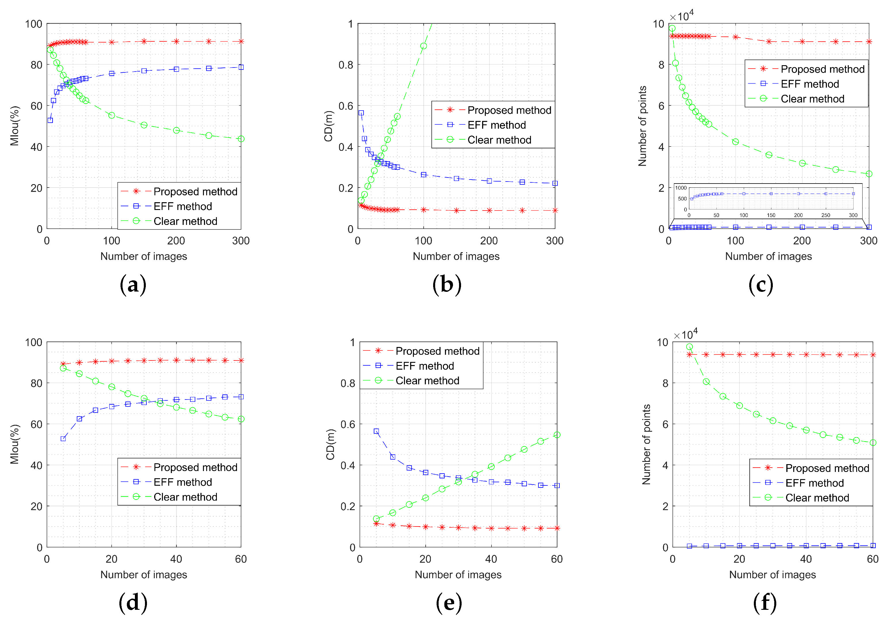
As shown in Figure 23, the performance metrics of the three methods vary with the number of image pairs, which varies from 5 to 60. For convenient viewing and analysis, Figure 23d–f show the reconstruction performance variation. It is obvious that both the OC-V3R-OI method and the EFF method exhibit higher precision and similarity to the original model as the number of images increases. Conversely, the clear method accumulates errors with the increasing number of images, resulting in decreased precision and similarity. The voxel representation used in the OC-V3R-OI method and the clear method allows for more model points and a denser representation, while the EFF method remains relatively sparse.
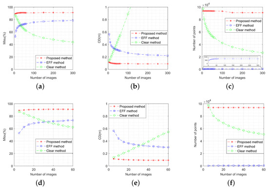
Figure 23.
Performance comparison of the three methods with different number of images: (a) variation of model intersection over union; (b) variation of Chamfer distance; (c) variation of number of points; (d) variation of model intersection over union when the image number varies from 5 to 60; (e) variation of Chamfer distance when the image number varies from 5 to 60; (f) variation of number of points when the image number varies from 5 to 60.
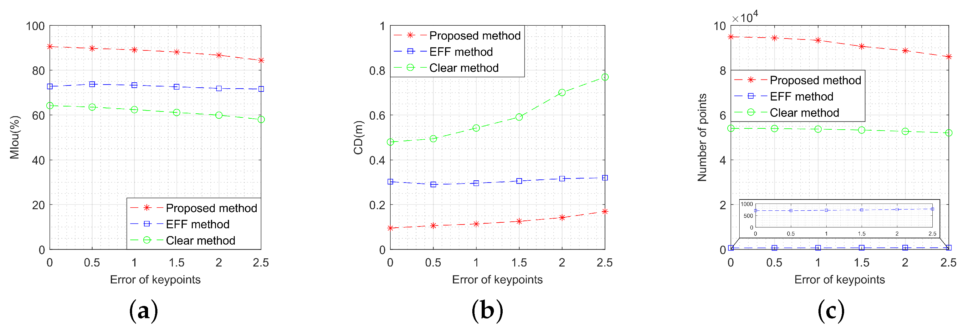
As depicted in Figure 24, the performance metrics of the three methods vary with key point position deviation. It is observed that both the OC-V3R-OI method and the clear method experience a decrease in performance to some extent due to the introduction of key point errors. However, the OC-V3R-OI method still demonstrates better performance in precision, similarity, and density when evaluated against the EFF method and the clear method.
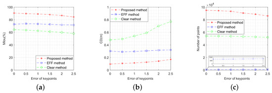
Figure 24.
Performance comparison of the three methods with different errors of key points: (a) variation of model intersection over union; (b) variation of Chamfer distance; (c) variation of number of points.
As depicted in Figure 25, the performance metrics of the three methods vary with the image SNR. Relative to the EFF method and the clear method, the OC-V3R-OI method is less dependent on SNR and exhibits stronger robustness, demonstrating better performance in precision, similarity, and density.
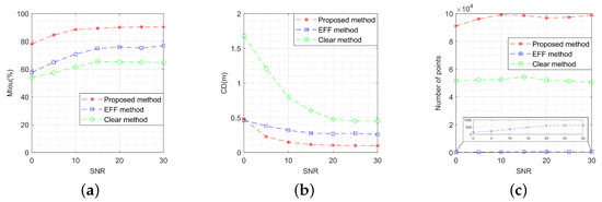
Figure 25.
Performance comparison of the three methods with different signal-to-noise ratio: (a) variation of model intersection over union; (b) variation of Chamfer distance; (c) variation of number of points.
A further qualitative analysis of the strengths and weaknesses of each method under various conditions, such as target motion characteristics, target structural features, imaging quantity, and imaging quality, are as follows:
- Target motion characteristics: The OC-V3R-OI method and EFF method exhibit superior performance in handling dynamic targets, maintaining high-quality reconstruction even under rapid motion. Both the clear method and the unaligned method struggle to adapt to such scenarios, resulting in reduced performance in moving target reconstruction.
- Target structural features: The voxel-based representation enhances the OC-V3R-OI method, clear method, and unaligned method in terms of information retention. In contrast, the sparsity of the EFF method may lead to the loss of critical information in certain applications, particularly when complex target structures are involved.
- Imaging quantity conditions: Both the OC-V3R-OI method and EFF method are adaptable to varying image quantities, effectively integrating image features to maintain reconstruction accuracy. The clear method, however, provides only basic reconstruction when data are sparse, and may not meet the precision requirements in high-demand applications. The unaligned method, on the other hand, suffers from cumulative errors as the number of images increases, making it unsuitable for scenarios with larger image datasets.
- Imaging quality conditions: The OC-V3R-OI method, clear method, and unaligned method all leverage the features of mask images directly, fully exploiting the advantages of deep networks in processing low-signal-to-noise-ratio images. The EFF method, however, is more affected by noise, resulting in sparser reconstructions that fail to meet accuracy requirements, particularly in challenging imaging conditions.
In summary, the OC-V3R-OI method demonstrates consistently high and stable performance throughout the entire experimental process in both quantitative and qualitative analyses.
6. Results
Optical and ISAR imaging are two important means for space target surveillance and perception, which have been extensively researched and explored separately for decades. In order to fully exploit the capabilities of multi-sensor joint observation, overcome the limitation of target motion type, and achieve comprehensive fusion of heterogeneous information, a 3-D reconstruction method, OC-V3R-OI, is proposed due to the alignment and fusion of simultaneously observed optical and ISAR images. The joint optical-and-ISAR COS is designed to simultaneously observe the space target. The image features are extracted by utilizing the HRNet, and the projection geometry is derived in detail to support the correction of the image offset between heterogeneous images and the spatial offset between asynchronous observations. By employing VTM-GL, dense 3-D reconstruction results, including the attitude information, are obtained.
Compared to traditional methods, the OC-V3R-OI method offers significant advantages. While the traditional EFF method can handle targets with arbitrary motion types, their reconstruction results are often sparse, and important target details are easily lost. The clear method is only suitable for scenarios with limited data and lower accuracy requirements. The unaligned method is effective only under ideal target motion and imaging conditions. In contrast, the OC-V3R-OI method successfully overcomes these issues through precise image alignment, spatial offset correction, and the VTM-GL mechanism.
Furthermore, the method proposed in this study maintains high reconstruction accuracy even when handling damaged or deformed spatial targets. This is made possible by its advanced feature extraction, flexible key point extraction strategy, and the effective use of global information through the VTM-GL method. This ensures that even with severely damaged target structures, the reconstruction results remain reliable.
Although the method has demonstrated its effectiveness and robustness in experiments, there are still some challenges. First, despite HRNet’s outstanding performance in feature extraction, the quality of the reconstruction can still be affected under extreme observational conditions, particularly when the number of images is limited or of low quality. Future research could further explore ways to enhance the method’s robustness in such complex environments. Additionally, we plan to explore the use of fewer images for 3D reconstruction and investigate more refined key point and mask feature extraction methods.
7. Conclusions
The OC-V3R-OI method proposed in this paper successfully overcomes the limitations of traditional EFF method in the 3-D reconstruction of spatial targets, particularly addressing issues related to target motion types and missing attitude information. By effectively integrating optical and ISAR images, this method resolves both image offset and spatial offset correction problems, achieving more precise and dense three-dimensional reconstruction results. Compared to traditional ISAR-based 3D reconstruction methods, the OC-V3R-OI method not only overcomes the constraints of motion types but also provides more reliable and complete reconstruction outcomes in complex scenarios. The combined advantages of optical and ISAR imaging enable the method to simultaneously capture both structural and attitude information of spatial targets. With the application of the VTM-GL method, reconstruction accuracy is significantly improved, further validating the effectiveness and robustness of this approach. In the future, as image quantity decreases and key point extraction methods are optimized, the OC-V3R-OI method will be able to deliver more efficient and precise 3D reconstruction solutions under increasingly complex and variable observational conditions.
Author Contributions
Conceptualization, W.Z.; methodology, W.Z. and L.L.; validation, W.Z.; formal analysis, W.Z. and Z.W.; investigation, W.Z., L.L. and R.D.; writing—original draft preparation, W.Z.; writing—review and editing, W.Z., L.L., R.D., Z.W., R.S. and F.Z.; visualization, W.Z.; supervision, F.Z.; project administration, W.Z.; funding acquisition, L.L. and F.Z. All authors have read and agreed to the published version of the manuscript.
Funding
This work was supported in part by the National Natural Science Foundation of China under Grant 62425113 and Grant 62401445; in part by the Postdoctoral Fellowship Program of CPSF (Program No. GZC20232048); in part by the Foundation of China for the Central Universities (Project No. XJSJ24008); and in part by the Innovation Fund of Xidian University.
Data Availability Statement
The original contributions presented in the study are included in the article, further inquiries can be directed to the corresponding author.
Acknowledgments
The authors thank the anonymous reviewers for their valuable comments to improve the paper quality.
Conflicts of Interest
The authors declare no conflicts of interest.
Abbreviations
The following abbreviations are used in this manuscript:
| ISAR | inverse synthetic aperture radar |
| 2-D | two-dimensional |
| 3-D | three-dimensional |
| 6D-ICP | six degree iterative closest point |
| InISAR | interferometric inverse synthetic aperture radar |
| LOS | line of sight |
| PSO | particle swarm optimization |
| EFF | extended factorization framework |
| COS | co-location observation system |
| VTM-GL | voxel trimming mechanism based on growth learning |
| CPI | coherent processing interval |
| MCS | measurement coordinate system |
| OCS | orbital coordinate system |
References
- Pi, Y.; Li, X.; Yang, B. Global Iterative Geometric Calibration of a Linear Optical Satellite Based on Sparse GCPs. IEEE Trans. Geosci. Remote Sens. 2020, 58, 436–446. [Google Scholar] [CrossRef]
- Gong, R.; Wang, L.; Wu, B.; Zhang, G.; Zhu, D. Optimal Space-Borne ISAR Imaging of Space Objects with Co-Maximization of Doppler Spread and Spacecraft Component Area. Remote Sens. 2024, 16, 1037. [Google Scholar] [CrossRef]
- Liu, X.w.; Zhang, Q.; Jiang, L.; Liang, J.; Chen, Y.j. Reconstruction of Three-Dimensional Images Based on Estimation of Spinning Target Parameters in Radar Network. Remote Sens. 2018, 10, 1997. [Google Scholar] [CrossRef]
- Shao, S.; Liu, H.; Yan, J. Integration of Imaging and Recognition for Marine Targets in Fast-Changing Attitudes With Multistation Wideband Radars. IEEE Trans. Aerosp. Electron. Syst. 2024, 60, 1692–1710. [Google Scholar] [CrossRef]
- Chen, S.Y.; Hsu, K.H.; Kuo, T.H. Hyperspectral Target Detection-Based 2-D–3-D Parallel Convolutional Neural Networks for Hyperspectral Image Classification. IEEE J. Sel. Top. Appl. Earth Obs. Remote Sens. 2024, 17, 9451–9469. [Google Scholar] [CrossRef]
- Chen, W.; Chen, H.; Yang, S. 3D Point Cloud Fusion Method Based on EMD Auto-Evolution and Local Parametric Network. Remote Sens. 2024, 16, 4219. [Google Scholar] [CrossRef]
- Liu, L.; Zhou, Z.; Zhou, F.; Shi, X. A New 3-D Geometry Reconstruction Method of Space Target Utilizing the Scatterer Energy Accumulation of ISAR Image Sequence. IEEE Trans. Geosci. Remote Sens. 2020, 58, 8345–8357. [Google Scholar] [CrossRef]
- Kucharski, D.; Kirchner, G.; Koidl, F.; Fan, C.; Carman, R.; Moore, C.; Dmytrotsa, A.; Ploner, M.; Bianco, G.; Medvedskij, M.; et al. Attitude and Spin Period of Space Debris Envisat Measured by Satellite Laser Ranging. IEEE Trans. Geosci. Remote Sens. 2014, 52, 7651–7657. [Google Scholar] [CrossRef]
- Koshkin, N.; Korobeynikova, E.; Shakun, L.; Strakhova, S.; Tang, Z. Remote Sensing of the EnviSat and Cbers-2B satellites rotation around the centre of mass by photometry. Adv. Space Res. 2016, 58, 358–371. [Google Scholar] [CrossRef]
- Pittet, J.N.; Šilha, J.; Schildknecht, T. Spin motion determination of the Envisat satellite through laser ranging measurements from a single pass measured by a single station. Adv. Space Res. 2018, 61, 1121–1131. [Google Scholar] [CrossRef]
- Zhang, H.; Wei, Q.; Jiang, Z. 3D Reconstruction of Space Objects from Multi-Views by a Visible Sensor. Sensors 2017, 17, 1689. [Google Scholar] [CrossRef]
- Wang, K.; Liu, H.; Guo, B.; Gao, Y. A 6D-ICP approach for 3D reconstruction and motion estimate of unknown and non-cooperative target. In Proceedings of the 2016 Chinese Control and Decision Conference (CCDC), Yinchuan, China, 28–30 May 2016; pp. 6366–6370. [Google Scholar] [CrossRef]
- Wang, G.; Xia, X.g.; Chen, V. Three-dimensional ISAR imaging of maneuvering targets using three receivers. IEEE Trans. Image Process. 2001, 10, 436–447. [Google Scholar] [CrossRef] [PubMed]
- Zhang, H.; Lin, Y.; Teng, F.; Feng, S.; Hong, W. Holographic SAR Volumetric Imaging Strategy for 3-D Imaging With Single-Pass Circular InSAR Data. IEEE Trans. Geosci. Remote Sens. 2023, 61, 1–16. [Google Scholar] [CrossRef]
- Luo, Y.; Deng, Y.; Xiang, W.; Zhang, H.; Yang, C.; Wang, L. Radargrammetric 3D Imaging through Composite Registration Method Using Multi-Aspect Synthetic Aperture Radar Imagery. Remote Sens. 2024, 16, 523. [Google Scholar] [CrossRef]
- Yang, X.; Sheng, W.; Xie, A.; Zhang, R. Rotational Motion Compensation for ISAR Imaging Based on Minimizing the Residual Norm. Remote Sens. 2024, 16, 3629. [Google Scholar] [CrossRef]
- Liu, L.; Zhou, F.; Bai, X.R.; Tao, M.L.; Zhang, Z.J. Joint Cross-Range Scaling and 3D Geometry Reconstruction of ISAR Targets Based on Factorization Method. IEEE Trans. Image Process. 2016, 25, 1740–1750. [Google Scholar] [CrossRef] [PubMed]
- Zhao, L.; Wang, J.; Su, J.; Luo, H. Spatial Feature-Based ISAR Image Registration for Space Targets. Remote Sens. 2024, 16, 3625. [Google Scholar] [CrossRef]
- Gu, X.; Yang, X.; Liu, H.; Yang, D. Adaptive Granularity-Fused Keypoint Detection for 6D Pose Estimation of Space Targets. Remote Sens. 2024, 16, 4138. [Google Scholar] [CrossRef]
- Niedfeldt, P.C.; Ingersoll, K.; Beard, R.W. Comparison and Analysis of Recursive-RANSAC for Multiple Target Tracking. IEEE Trans. Aerosp. Electron. Syst. 2017, 53, 461–476. [Google Scholar] [CrossRef]
- Xu, D.; Bie, B.; Sun, G.C.; Xing, M.; Pascazio, V. ISAR Image Matching and Three-Dimensional Scattering Imaging Based on Extracted Dominant Scatterers. Remote Sens. 2020, 12, 2699. [Google Scholar] [CrossRef]
- Morita, T.; Kanade, T. A sequential factorization method for recovering shape and motion from image streams. IEEE Trans. Pattern Anal. Mach. Intell. 1997, 19, 858–867. [Google Scholar] [CrossRef]
- Liu, L.; Zhou, F.; Bai, X.; Paisley, J.; Ji, H. A Modified EM Algorithm for ISAR Scatterer Trajectory Matrix Completion. IEEE Trans. Geosci. Remote Sens. 2018, 56, 3953–3962. [Google Scholar] [CrossRef]
- Zhou, Z.; Liu, L.; Du, R.; Zhou, F. Three-Dimensional Geometry Reconstruction Method for Slowly Rotating Space Targets Utilizing ISAR Image Sequence. Remote Sens. 2022, 14, 1144. [Google Scholar] [CrossRef]
- Zhou, Z.; Jin, X.; Liu, L.; Zhou, F. Three-Dimensional Geometry Reconstruction Method from Multi-View ISAR Images Utilizing Deep Learning. Remote Sens. 2023, 15, 1882. [Google Scholar] [CrossRef]
- Liu, A.; Zhang, S.; Zhang, C.; Zhi, S.; Li, X. RaNeRF: Neural 3-D Reconstruction of Space Targets From ISAR Image Sequences. IEEE Trans. Geosci. Remote Sens. 2023, 61, 1–15. [Google Scholar] [CrossRef]
- Zhou, Y.; Zhang, L.; Cao, Y.; Huang, Y. Optical-and-Radar Image Fusion for Dynamic Estimation of Spin Satellites. IEEE Trans. Image Process. 2020, 29, 2963–2976. [Google Scholar] [CrossRef]
- Du, R.; Liu, L.; Bai, X.; Zhou, Z.; Zhou, F. Instantaneous Attitude Estimation of Spacecraft Utilizing Joint Optical-and-ISAR Observation. IEEE Trans. Geosci. Remote Sens. 2022, 60, 1–14. [Google Scholar] [CrossRef]
- Zhou, Y.; Zhang, L.; Xing, C.; Xie, P.; Cao, Y. Target Three-Dimensional Reconstruction From the Multi-View Radar Image Sequence. IEEE Access 2019, 7, 36722–36735. [Google Scholar] [CrossRef]
- Long, B.; Tang, P.; Wang, F.; Jin, Y.Q. 3-D Reconstruction of Space Target Based on Silhouettes Fused ISAR–Optical Images. IEEE Trans. Geosci. Remote Sens. 2024, 62, 1–19. [Google Scholar] [CrossRef]
- Zhou, W.; Liu, L.; Du, R.; Yang, Y.; Zhou, F. A novel 3-D geometry reconstruction method of space target based on joint optical-and-ISAR observation. In Proceedings of the IET International Radar Conference (IRC 2023), Chongqing, China, 3–5 December 2023; Volume 2023, pp. 3231–3236. [Google Scholar] [CrossRef]
- Liu, X.W.; Zhang, Q.; Luo, Y.; Lu, X.; Dong, C. Radar Network Time Scheduling for Multi-Target ISAR Task With Game Theory and Multiagent Reinforcement Learning. IEEE Sens. J. 2021, 21, 4462–4473. [Google Scholar] [CrossRef]
- Wang, D.; Zhang, Q.; Luo, Y.; Liu, X.; Ni, J.; Su, L. Joint Optimization of Time and Aperture Resource Allocation Strategy for Multi-Target ISAR Imaging in Radar Sensor Network. IEEE Sens. J. 2021, 21, 19570–19581. [Google Scholar] [CrossRef]
- Wang, J.; Li, Y.; Song, M.; Huang, P.; Xing, M. Noise Robust High-Speed Motion Compensation for ISAR Imaging Based on Parametric Minimum Entropy Optimization. Remote Sens. 2022, 14, 2178. [Google Scholar] [CrossRef]
- Liu, Y.; Yi, D.; Wang, Z. Coordinate transformation methods from the inertial system to the centroid orbit system. Aerosp. Control 2007, 25, 4–8. [Google Scholar]
- Ramalingam, S.; Sturm, P. A Unifying Model for Camera Calibration. IEEE Trans. Pattern Anal. Mach. Intell. 2017, 39, 1309–1319. [Google Scholar] [CrossRef]
- Ning, Q.; Wang, H.; Yan, Z.; Wang, Z.; Lu, Y. A Fast and Robust Range Alignment Method for ISAR Imaging Based on a Deep Learning Network and Regional Multi-Scale Minimum Entropy Method. Remote Sens. 2024, 16, 3677. [Google Scholar] [CrossRef]
- Liu, C.; Luo, Y.; Yu, Z. A Robust Translational Motion Compensation Method for Moving Target ISAR Imaging Based on Phase Difference-Lv’s Distribution and Auto-Cross-Correlation Algorithm. Remote Sens. 2024, 16, 3554. [Google Scholar] [CrossRef]
- Zhao, S.; Luo, Y.; Zhang, T.; Guo, W.; Zhang, Z. A domain specific knowledge extraction transformer method for multisource satellite-borne SAR images ship detection. ISPRS J. Photogramm. Remote Sens. 2023, 198, 16–29. [Google Scholar] [CrossRef]
- Liu, Z.; Li, Z.; Liang, Y.; Persello, C.; Sun, B.; He, G.; Ma, L. RSPS-SAM: A Remote Sensing Image Panoptic Segmentation Method Based on SAM. Remote Sens. 2024, 16, 4002. [Google Scholar] [CrossRef]
- Wang, J.; Sun, K.; Cheng, T.; Jiang, B.; Deng, C.; Zhao, Y.; Liu, D.; Mu, Y.; Tan, M.; Wang, X.; et al. Deep High-Resolution Representation Learning for Visual Recognition. IEEE Trans. Pattern Anal. Mach. Intell. 2021, 43, 3349–3364. [Google Scholar] [CrossRef]
- Franceschetti, G.; Iodice, A.; Riccio, D. A canonical problem in electromagnetic backscattering from buildings. IEEE Trans. Geosci. Remote Sens. 2002, 40, 1787–1801. [Google Scholar] [CrossRef]
- Boag, A. A fast physical optics (FPO) algorithm for high frequency scattering. IEEE Trans. Antennas Propag. 2004, 52, 197–204. [Google Scholar] [CrossRef]
- Auer, S.; Hinz, S.; Bamler, R. Ray-Tracing Simulation Techniques for Understanding High-Resolution SAR Images. IEEE Trans. Geosci. Remote Sens. 2010, 48, 1445–1456. [Google Scholar] [CrossRef]
- Kulpa, K.S.; Samczyński, P.; Malanowski, M.; Gromek, A.; Gromek, D.; Gwarek, W.; Salski, B.; Tański, G. An Advanced SAR Simulator of Three-Dimensional Structures Combining Geometrical Optics and Full-Wave Electromagnetic Methods. IEEE Trans. Geosci. Remote Sens. 2014, 52, 776–784. [Google Scholar] [CrossRef]
- Fan, H.; Su, H.; Guibas, L. A Point Set Generation Network for 3D Object Reconstruction from a Single Image. In Proceedings of the 2017 IEEE Conference on Computer Vision and Pattern Recognition (CVPR), Honolulu, HI, USA, 21–26 July 2017; pp. 2463–2471. [Google Scholar] [CrossRef]


Disclaimer/Publisher’s Note: The statements, opinions and data contained in all publications are solely those of the individual author(s) and contributor(s) and not of MDPI and/or the editor(s). MDPI and/or the editor(s) disclaim responsibility for any injury to people or property resulting from any ideas, methods, instructions or products referred to in the content. |
© 2025 by the authors. Licensee MDPI, Basel, Switzerland. This article is an open access article distributed under the terms and conditions of the Creative Commons Attribution (CC BY) license (https://creativecommons.org/licenses/by/4.0/).