Article

3D Seismic Attribute Conditioning Using Multiscale Sheet-Enhancing Filtering

1
School of Information and Software Engineering, University of Electronic Science and Technology of China, Chengdu 610054, China
2
School of Resources and Environment and Center for Information Geoscience, University of Electronic Science and Technology of China, Chengdu 611731, China
3
School of Information and Communication Engineering and Center for Information Geoscience, University of Electronic Science and Technology of China, Chengdu 611731, China
*
Author to whom correspondence should be addressed.
Remote Sens. 2025, 17(2), 278; https://doi.org/10.3390/rs17020278
Submission received: 5 December 2024 / Revised: 8 January 2025 / Accepted: 11 January 2025 / Published: 14 January 2025

Abstract

:
Seismic coherence attributes are valuable for identifying structural features, but they often face challenges due to significant background noise and non-feature-related stratigraphic discontinuities. To address this, it is necessary to apply attribute conditioning to the coherence to enhance the visibility of these structures. The primary challenge of attribute conditioning lies in finding a concise structural representation that isolates only the true interpretive features while effectively removing noise and stratigraphic interference. In this study, we choose sheet-like structures as this concise structural representation, as faults are typically characterized by their thin and narrow profiles. Inspired by multiscale Hessian-based filtering (MHF) and its application on vascular structure detection, we propose a method called anisotropic multiscale Hessian-based sheet-enhancing filtering (AMHSF). This method is specifically designed to extract and magnify sheet-like structures from noisy coherence images, with a novel enhancement function distinct from those traditionally used in vascular enhancement. The effectiveness of our AMHSF is demonstrated through experiments on both synthetic and real datasets, showcasing its potential to improve the identification of structural features in coherence images.

1. Introduction

Knowledge about seismic coherence attributes is critical to our understanding and quantification of fault interpretations, which is necessary for providing a quantitative analysis of linear discontinuities between seismic traces, allowing for swift fault detection. However, these attributes are prone to distortions caused by data noise and stratigraphic interference, both of which can manifest as discontinuities in 3D seismic images [1,2,3]. Consequently, attribute conditioning, a subtask of fault detection, focuses on enhancing the useful signals within the acquired data by effectively suppressing background noise and mitigating the impact of stratigraphic intervention. The central challenge in this process is distinguishing the true fault structures from the background coherent noise and stratigraphic interruption [4,5].
In our ongoing study, we focus on the attribute conditioning task, and therefore, extracting coherence attribute images from 3D seismic data are a preliminary step. Significant advancements have been made in generating coherence images by applying various attributes to analyze changes in seismic signals, including those based on the original amplitude [6,7,8,9,10,11,12,13,14], the first-order gradient (i.e., the border) [15,16,17,18,19], the second-order gradient (i.e., the shape) [20,21,22,23,24], and the third-order gradient (i.e., the shape variations) [25,26]. The first category quantifies lateral similarity between seismic traces through methods, such as cross-correlation [6], semblance [7], eigenstructure analysis [8,9,10,11,12], and variance [13,14]. The second category shifts the focus from trace similarity to the principal first-order gradient direction for each pixel in seismic images using the gradient structure tensor (GST). Examples of such methods include regular GST [15,16,17], directional GST [18], and robust GST [19]. The third category evaluates surface deformation by analyzing second-order gradient changes at specific points, commonly referred to as curvature [20,21,22,23,24]. Lastly, the fourth category measures the lateral variation of curvature along a surface, known as aberrancy [25,26], which represents third-order surface behavior. Despite these advanced methods, the presence of background noise and residual stratigraphy limits the effectiveness of seismic coherence attributes in detecting structural and stratigraphic features [27].
Until now, various effective techniques have been developed for the automatic detection of faults in 3D seismic coherence images, utilizing approaches such as fault-oriented smoothing [27,28,29,30,31,32], optimization algorithms [33,34,35], and deep learning models [4,36,37,38,39,40,41,42]. Fault-oriented smoothing enhances fault features by smoothing along fault strikes and dips, which is achieved by scanning all potential combinations of fault strike and dip angles [27,28,29,30,31,32]. Optimization algorithms, on the other hand, estimate fault surface using inverse methods, including techniques such as ant tracking [33], temporal–spatial staggered-grid finite difference forward algorithms [34], and dynamic programming [35]. Deep learning addresses fault detection as a pixel classification task, where each pixel is to be assigned a Boolean label, with neural networks like convolutional neural networks (CNNs) [4,36,37,38,39,40], U-Nets with Transformer modules [41], or Transformer-based models [42] being employed to solve the problem. It is worth noting that many contemporary methods integrate attribute conditioning and fault construction into a single, unified process for fault detection. However, the focus of this study is specifically on attribute conditioning.
Another method, known as multiscale Hessian-based filtering (MHF), is designed to model and enhance structures of interest, with the ultimate goal of segmenting them. A notable example of this is multiscale Hessian-based filtering for vascular structures (MHF4V) [43,44,45]. Considering the inherently sheet-like feature of faults, we introduce sheet-like structures for modeling fault and fracture features. Additionally, inspired by MHF4V, we propose anisotropic multiscale Hessian-based sheet-enhancing filtering (AMHSF) to enhance such structures in 3D coherence images and mitigate background noise and stratigraphic interruption. Utilizing anisotropic Gaussian filtering, we successfully filter out essential features, such as faults and fractures, from contaminated coherence images. Here, we summarize four advantages of our proposed method AMHSF:
(1)
Compatibility: The effectiveness of AMHSF reflies solely on the assumption that interpretative features conform to sheet-like structures. Thus, our AMHSF can effectively filter and enhance any sheet-like structure information within attribute images.
(2)
Accuracy: As a typical filter, AMHSF accurately isolates sheet-like structures from non-sheet-like ones in a non-iterative and deterministic manner, as long as the underlying assumption of sheet-like behavior is valid.
(3)
No Requirement for Additional Data: AMHSF does not necessitate any supplementary data (e.g., strike and dip information) beyond the coherence images, which further contributes to the precision of the filtering.
(4)
Simplicity of Implementation: AMHSF involves only three key stages with two post-processing stages, making it straightforward to implement.
Compared to the conventional MHF, two key distinctions make our method particularly effective for processing sheet-like structures. These distinctions, which represent the core contributions of our work, are summarized as follows:
(1)
AMHSF enables the precise isolation of relevant sheet-like features, such as faults and fractures, from noise-contaminated attribute images. To the best of our knowledge, we are among the first to introduce the sheet-like assumption and the corresponding AMHSF in seismic attribute analysis for the purpose of attribute conditioning in coherence images.
(2)
A major innovation of our proposed AMHSF is the development of a novel enhancement function specifically designed to highlight sheet-like structures in coherence images. This function is fundamentally different from the enhancement functions typically used in vascular structure enhancement.

2. Materials and Methods

This section is arranged as follows: Section 2.1 describes the design and details of our proposed method; Section 2.2 demonstrates our implementation details; and Section 2.3 presents the materials, i.e., the experimental data, used in our study and their relative processing.

2.1. Methods

2.1.1. Preliminaries

We begin by reviewing the essential preliminaries required to develop our method. Multiscale Hessian-based filtering (MHF) is commonly used to selectively amplify a particular profile or structure of local intensity by investigating the second-order intensity Hessian at any point in a 3D seismic attribute image [43,44,45]. Consider the coherence value of a 3D seismic attribute image, denoted as Y x , at the coordinate x = [ x 1 , x 2 , x 3 ] T , where x 1 , x 2 , and x 3 correspond to the coordinate values on inline, crossline, and timeline dimensions, respectively. At x and scale s, the Hessian matrix H of Y x is estimated via 3D Gaussian filtering and is expressed as a symmetric 3 × 3 matrix, whose elements are:
H i j x , s = s 2 Y x 2 x i x j G x , s , for i , j = 1 , 2 , 3 ,
where G x , s = 2 π s 3 3 / 2 exp x T x / 2 s 2 represents a three-variate Gaussian function, and ∗ denotes the convolution operation. Then, the eigenvalues of the Hessian matrix can be obtained by performing eigenvalue decomposition eig H λ i , i = 1 , 2 , 3 for each x . The enhancement based on the Hessian matrix can be interpreted as the response of an indicator function 1 E R : eig H x , s 0 , 1 , which is derived from a specific set of eigenvalue relations (ER). The indicator function is approximated using a smooth enhancement function V : eig H x , s R 0 + to capture variations in the target structures’ shape and intensity. The design of V is tailored to enhance elongated structures. A well-known example of such a function is Frangi’s in vascular enhancing [43], and it is defined as:
V F = 1 exp R A 2 2 α 2 1 exp S 3 2 2 κ 2 ,
where S 3 = λ 1 2 + λ 2 2 + λ 3 2 is a second-order measure of image structures, R A = λ 2 / λ 3 distinguishes between tubular and sheet-like structures, and parameters α and κ are thresholds controlling the sensitivity of measures R A and S , respectively. A detailed discussion of the enhancement functions can be found in [45]. Given the enhancement function V , a multiscale filter response measure F ( x ) is computed by maximizing over a range of scales s for each x as given by:
F ( x ) = sup V eig H ( x , s ) : s m i n s s m a x ,
where s m i n and s m a x are chosen based on the anticipated size range of the structures of interest. These bounds are manually set to capture the relevant structural features effectively.

2.1.2. Proposed Methods

Our goal is to extract sheet-like structures X sheet from the precomputed 3D coherence attribute image Y . Image derivatives play a crucial role in this process, as they encode both the border (first-order derivative) and shape (second-order derivative) information about the structures within the image. Specifically, eigenvalues extracted from the second-order derivative matrix (i.e., the Hessian matrix) can be utilized to derive geometrical structures, which can be characterized as sheet-like [35,46]. However, considering that residual strata inherently exhibit sheet-like behavior in the lateral direction as well, distinguishing faults from strata using conventional Hessian-based isotropic filtering, as reviewed in Section 2.1.1, is difficult.
To address this limitation, we propose the use ofanisotropic multiscale Hessian-based filtering (AMHF). This technique transforms strata into imperfect tubular structures by employing an elliptical Gaussian window, with the primary axis aligned along the timeline dimension. Notably, anisotropic Gaussian windows are commonly employed in the computation of coherence attributes, such as in GST [15,16,17]. Anisotropy is achieved by applying different scaling factors in the inline, crossline, and timeline directions [47]. An elliptical Gaussian aligned with the coordinate system is defined as:
G x ; σ i , σ c , σ t = 1 2 π σ i σ c σ t exp 1 2 x i σ i 2 + x c σ c 2 + x t σ t 2 ,
where σ i , σ c , and σ t represent the scales in the inline, crossline, and timeline directions, respectively. For AMHF, the key difference lies in the introduction of a new scale definition, given by:
a = { σ i ( ) , σ c ( ) , σ t ( ) } , [ K ] ,
where K is the number of scales and [ K ] denotes the set { 1 , 2 , 3 , , K } . With this, the anisotropic Hessian of Y x can be represented by a symmetric 3 × 3 matrix at x and scale  a :
H i j x , a = σ i ( ) σ c ( ) σ t ( ) Y x 2 x i x j G x ; σ i ( ) , σ c ( ) , σ t ( ) , for i , j = 1 , 2 , 3 .
The anisotropic Hessian matrix, as defined in Equation (6), encapsulates the shape information by capturing second-order variations within attribute images. In particular, the eigenvalues decomposition of the anisotropic Hessian matrix provides significant local detail, enabling the distinction between various structures, such as blob-like, tube-like, sheet-like, and noisy features within the attribute data. Figure 1 and Table 1 present a comprehensive correspondence between the eigenvalues of the Hessian matrix and the orientation of image structures. Moreover, these visualizations elucidate the relationship between seismic image attributes, local structural features, and the associated Hessian eigenvalues, as summarized in Figure 1 and Table 1. This relationship serves as a key framework for interpreting the geometrical characteristics of seismic data based on local eigenvalue behavior:
(1)
Sheet-like Structures: Following the approach in [46,47,48,49], we assume that the underlying features exhibit sheet-like behavior at every voxel in Figure 1. When this assumption holds, we define a ratio to distinguish sheet-like structures from other patterns:
R sheet = λ 3 λ 2 .
(2)
Tubular Structures: As discussed earlier, residual stratigraphy can be modeled as a tubular structure within the Hessian matrix, governed by an elliptical Gaussian window. Equation (2) provides a mechanism to effectively isolate tubular structures from other geometrical forms [43].
(3)
Blob-like Structures: Blob-like features are typically indicative of noise. The following equation serves to differentiate blob-like structures from other types [43]:
R blob = 2 λ 3 λ 2 λ 1 λ 3 .
(4)
Noisy Structures: In this case, random noise is found in a structureless state, which is represented by half the maximum Frobenius norm R noise [43]:
R noise = λ 1 2 + λ 2 2 + λ 3 2 .
It is worth noting that we focus on developing a multiscale sheetness measure that selectively enhances sheet-like structures rather than filtering out each individual structure. This measure is subsequently utilized to derive a deformable surface that halts at the feature boundaries. Owing to the multiscale approach, the sheetness measure is designed to achieve its maximum value when evaluated at the scale corresponding to the characteristic radius of the sheet objects. Inspired by vascular enhancement techniques [43,44,45], we propose a multiscale sheetness measure F ( x ) as the maximum response over all scales a , at which the Hessian derivatives are computed, to emphasize sheet-like structures:
F ( x ) = sup V eig H x , a : K ,
where V · is the sheet-like structure enhancement function, which is to be discussed. This measure is employed to construct a deformable surface that accurately conforms to feature boundaries. However, due to the distinct nature of coherence images and the specific characteristics of their extracted features, the enhancement function of our proposed AMHSF differs significantly from conventional sheet-enhancing methods. As a result, a specialized enhancement function was developed to suit the requirements of our attribute conditioning task.
The enhancement of structural features is contingent on their relative brightness with respect to the surrounding background. Accordingly, a generalized enhancement function can be established by redefining the Hessian eigenvalues to reflect the intensity contrast between the target structures and the background, irrespective of whether these features appear brighter or darker. Each eigenvalue λ i , i = 1 , 2 , 3 , is redefined as follows:
λ i = λ i bright structures on a dark background , λ i dark structures on a bright background .
To enhance sheet-like structures in a 3D attribute image, the function V should indicate the following Hessian eigenvalue relations:
1 E R : λ 1 λ 2 0 λ 3 λ 1 , 2 .
Building upon Equation (12), we begin the construction of our enhancement function. Drawing inspiration from [50], we have adapted the original Sato enhancement function to develop a more refined version, specifically designed to accentuate the sheet-like structural features illustrated in Figure 1. This modification is formally expressed as follows:
V sheet = λ 3 R sheet max R sheet γ ,
where the parameter γ controls the sensitivity to sheet-like structures, with typical values being to 0.5 or 1. The first term reflects the magnitude and the second represents the likelihood of a sheet and rounded structure. In regions where the feature is neither sheet-like nor structured, the second term diminishes towards 0, as R sheet max R sheet 0 . To further mitigate the influence of rounded structures, the proposed enhancement function is computed as:
V a = λ 3 R sheet max R sheet γ if v s . > 0 , 0 otherwise ,
for each pixel v in V sheet . Moreover, we propose another appropriate function to enhance sheet-like structures, which is revised from [49] in the same way as Equation (14). Correspondingly, the enhancement function is redefined as:
V a = λ 3 λ 2 λ 1 if v s . > 0 , 0 otherwise .
Notably, both enhancement function (14) and (15) are effective for our task, which is verified in Section 3. In a specific implementation, it is necessary to choose one from these two functions (or any future functions that may be proposed). After performing the aforementioned calculations on each voxel across multiple scales in 3D attribute images, the scales are combined using the following equation:
V ^ = max V a , [ K ] .
This process selects the maximum Hessian response at each voxel across all scales, which can effectively integrate various apertures.

2.2. Implementation

Similar to the MHF, our proposed AMHSF offers easy and efficient implementation of advanced attribute conditioning techniques. The computational workflow of our work typically comprises three key stages: construction of the Hessian matrix, matrix eigenvalue solving, and the enhancing of the sheet-like structures. These steps are performed iteratively. The process is repeated across a finite set of scales, selected by the user to encompass the maximum range of feature thicknesses in the coherent image.
In our method, the approach for achieving computational efficiency is similar to the standard MHF. For a given coherent attribute image Y and three directional scales σ i , σ c , and σ t , the first step involves constructing the anisotropic Hessian matrix H i j using the function AniHessian ( · ) , which implements Equation (6). Subsequently, the eigenvalues λ i of the matrix H i j are computed via eig 3 volume ( · ) . The function SheetEnhancing ( · ) is then applied to determine the sheetness measure for the input attribute image Y . Among these steps, the most computationally intensive tasks within a single iteration are the formation of the Hessian matrix and the estimation of its eigenvalues. Furthermore, the use of recursive Gaussian filtering [51,52] and analytical eigenvalue decomposition [53] significantly reduces the overall computational complexity.
Through experiments, we discovered that the sheet-enhancing process may introduce small artifacts, or “burrs”, which necessitates post-processing to improve the overall visual quality of the resulting images. A key aspect of this refinement involves eliminating points with low absolute values. The artifacts caused by these points typically emerge in non-sheet-like structures and, if left unaddressed, may compromise the accurate interpretation of the coherence image. Fortunately, their characteristic of having significantly lower absolute values compared to genuine sheet-like structures makes them identifiable for removal. This refinement is given by:
V rfn = v s . if v > θ , 0 otherwise ,
for each point v of V ^ . Here, the parameter θ is the removal threshold. Another critical step involves smoothing along the dominant orientation of features without crossing them. In this context, we employ anisotropic diffusion [54] to perform smoothing on the attribute-conditioned images, implemented using the following Matlab notation: V diff = imdiffusefilt ( V ^ ) . The function imdiffusefilt ( · ) aims to perform edge-aware noise reduction through anisotropic diffusion. While anisotropic diffusion may not be the optimal method for our task, a thorough examination of alternative approaches falls outside the scope of this study and is reserved for future work. The complete methodology is outlined in detail in Algorithm 1.
Algorithm 1 AMHSF
Require:  Y , σ i , σ c , σ t , θ .
Ensure:  X sheet .
1:
for  = 1 , , K  do
2:
     H i j AniHessian x , a .                 ▹ constructing anisotropic Hessian matrix
3:
     λ i eig 3 volume H i j .                                           ▹ matrix eigenvalue solving
4:
     V SheetEnhancing λ i .                          ▹ enhancing sheet-like structures
5:
end for
6:
V ^ = max V .                        ▹ taking the maximum value as the supremum
7:
V diff imdiffusefilt ( V ^ ) .                                                      ▹ anisotropic diffusion
8:
V rfn absremoval V diff , θ .                       ▹ removing low-absolute-value points
9:
X sheet V rfn .
In our implementation, the coherence image is convolved with the derivatives of anisotropic Gaussian kernels, characterized by the deviations σ i , σ c , and σ t , in order to compute the Hessian matrix. Therefore, these parameters must be precisely tuned to ensure the optimal accuracy in attribute conditioning. Moreover, the threshold θ in low-absolute-value points removal also needs careful calibration: a value that is too large risks discarding valuable information, while a value that is too small renders the removal process ineffective. The parameter tuning process requires numerous computationally intensive experiments. Conducting a grid search across all possible parameters is typically impractical. Instead, a greedy approach is often adopted, where only one or a few components are adjusted at a time. Through iterative experimentation, we provide the current optimal set of parameters for the synthetic and real datasets employed in this study, as provided in Table 2.

2.3. Data and Data Processing

In this study, our work is based on an open synthetic 3D fault dataset and two real-world datasets, Opunake-3D and Parihaka-3D. The synthetic dataset, released by Wu et al. in FaultSeg [4], was initially used to train a deep neural network (DNN) for fault detection. It consists of 220 pairs of synthetic seismic volumes with corresponding ground truth faults as labels. The dataset is divided into a training set of 200 samples and a validation set of 20 samples. Each data cube has dimensions of 128 × 128 × 128 (inline, crossline, and timeline). We randomly selected two samples from the training set (samples with IDs 69 and 125) and introduced 10 dB Gaussian noise to generate noisy data. We then computed the variance coherence, the input to our proposed method, for both the original noise-free and noisy volumes. The slicing window size was set to 3 × 3 × 3 to compute the variance coherence, and this window size remained consistent across experiments.
The Opunake-3D dataset, provided by New Zealand Crown Minerals, is a prestack, time-migrated dataset. The full dataset is a 9.68 GB SEG-Y file, and processing the entire dataset would be time-consuming and unnecessary for demonstrating the feasibility of our method. Therefore, we segmented the data into subcubes with dimensions of 400 × 200 × 100 (inline, crossline, and timeline) and randomly selected two subcubes for the variance coherence computation. No additional noise was introduced, as the real-world data are inherently noisy due to the collection process.
The Parihaka-3D dataset, also from New Zealand Crown Minerals, includes a full angle stack along with near, mid, and far stacks. The data have undergone final anisotropic, Kirchhoff prestack, and time migration. We selected the full angle stack for analysis, as it provides the most comprehensive view of the data. The same processing steps applied to the Opunake-3D dataset were followed: the data were divided into 400 × 200 × 100 subcubes and the variance coherence was computed using a 3 × 3 × 3 slicing window.

3. Results

In this section, we evaluate the feasibility of our AMHSF methodology and present both qualitative and quantitative results. A more comprehensive description and analysis are provided for the experiments conducted on the synthetic dataset, as it provides ground truth and allows for a clearer illustration of AMHSF capability.

3.1. Experimental Results with the Synthetic 3D Dataset

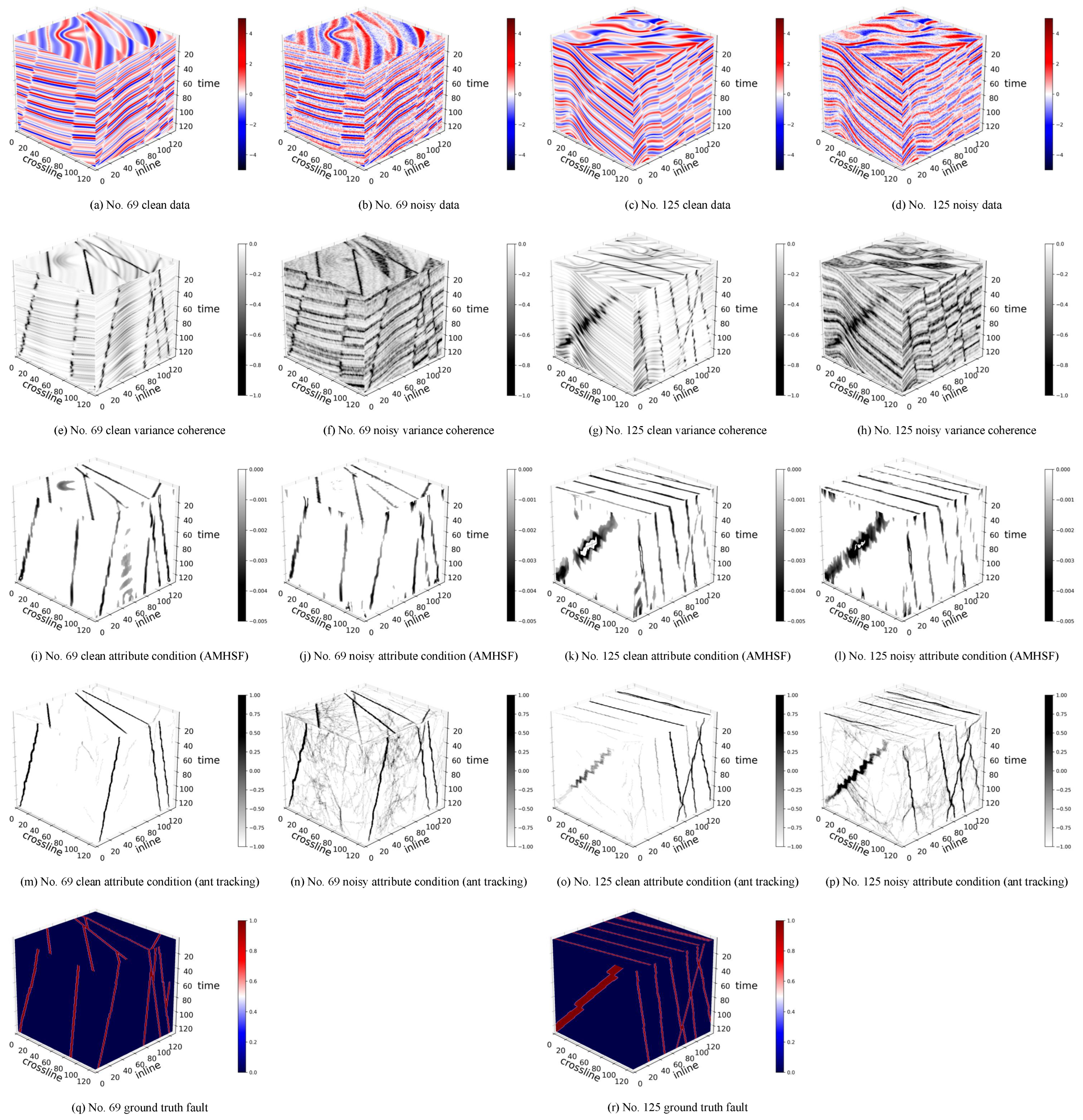
Figure 2 presents the experimental results on the synthetic dataset in 3D. The first column (subfigures (a), (e), (i), and (m)) shows the 3D cubes of the original noise-free seismic amplitude, the variance coherence, the attribute condition (obtained results), and the ground truth fault of the No. 69 sample. Here, the ground truth fault is the label to evaluate the performance of our method. The subfigures in the second column (subfigures (b), (f), and (j)) are the seismic amplitude, the variance coherence, and the attribute condition (obtained results), respectively. The last two columns are the results of the No. 125 sample in the same illustrating sequence. It is important to acknowledge that the occasional blank spotted in the attribute conditioning results, e.g., the blank in subfigure (k) is likely attributable to a compatibility issue between the plotting library Matplotlib and our Python environment, rather than a flaw in our methodology (this compatibility issue will make 3D plotting background visible, leading to the so-called blanks, but it does not impact the result interpretation).
Comparing the second, the third, and the last rows, i.e., the variance coherence, resulting attribute conditions, and the ground truth, the horizon lines shown in the variance coherence (subfigures (e), (f), and (h)) are clearly removed in the results obtained by our AMHSF. Moreover, the ground truth faults are successfully extracted and enhanced through our method as expected. This difference shows that our proposed AMHSF is effective to enhance the valuable sheet-like information and is powerful in removing background noise and stratigraphic anomalies. Furthermore, the faults are clearly discernible in both the original noise-free data and the noisy data when comparing subfigures (i) with (j) and (k) with (l). In contrast, the variance coherence effectively highlights these faults only in noise-free conditions (subfigures (e) and (g)), but fails to do so when noisy (subfigures (f) and (h)). This indicates that our method is robust enough to withstand a certain degree of noise and anomalies. Lastly, there are the artifacts found in attribute conditioning results (subfigures (i), (j), (k), and (l)). Removing them will be left to future work.
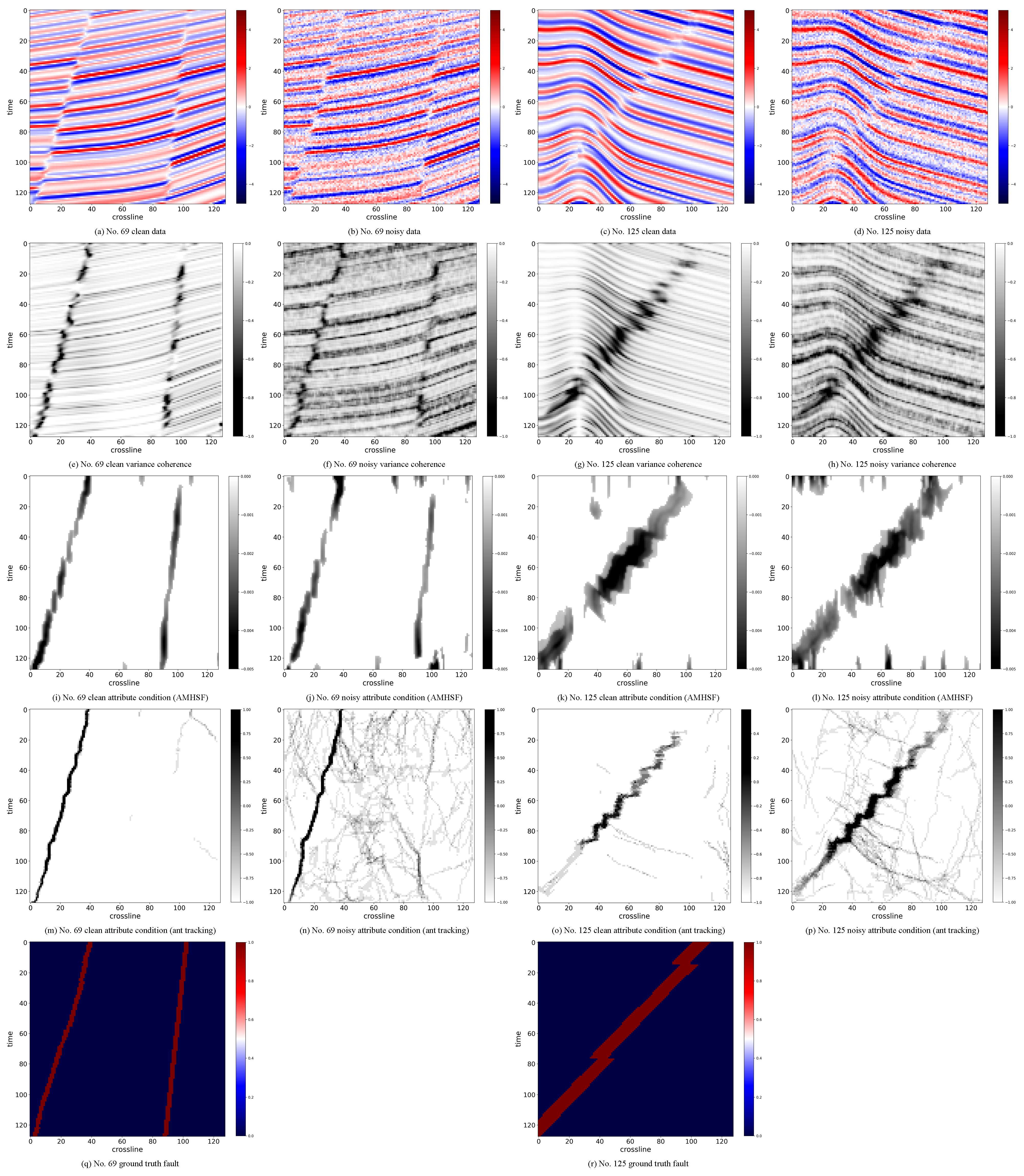
According to our survey in Section 1, we select the classic attribute conditioning algorithm ant tracking [33], which is the current state-of-the-art modeling-based method and has been implemented in commercial software, as the baseline for comparison. The results obtained by ant tracking are presented in the fourth row of Figure 2 and Figure 3. Comparing our AMHSF with ant tracking, we observe that while ant tracking yields finer results, it fails to highlight all the faults present in the attribute images. In contrast, our method successfully identifies all fault information, demonstrating a clear advantage in this regard. Figure 3 presents the 20th inline slices of the experimental results, providing a more detailed representation of our results. Although these are just sampled slices from the 3D cubes, similar conclusion can still be drawn from these subfigures.
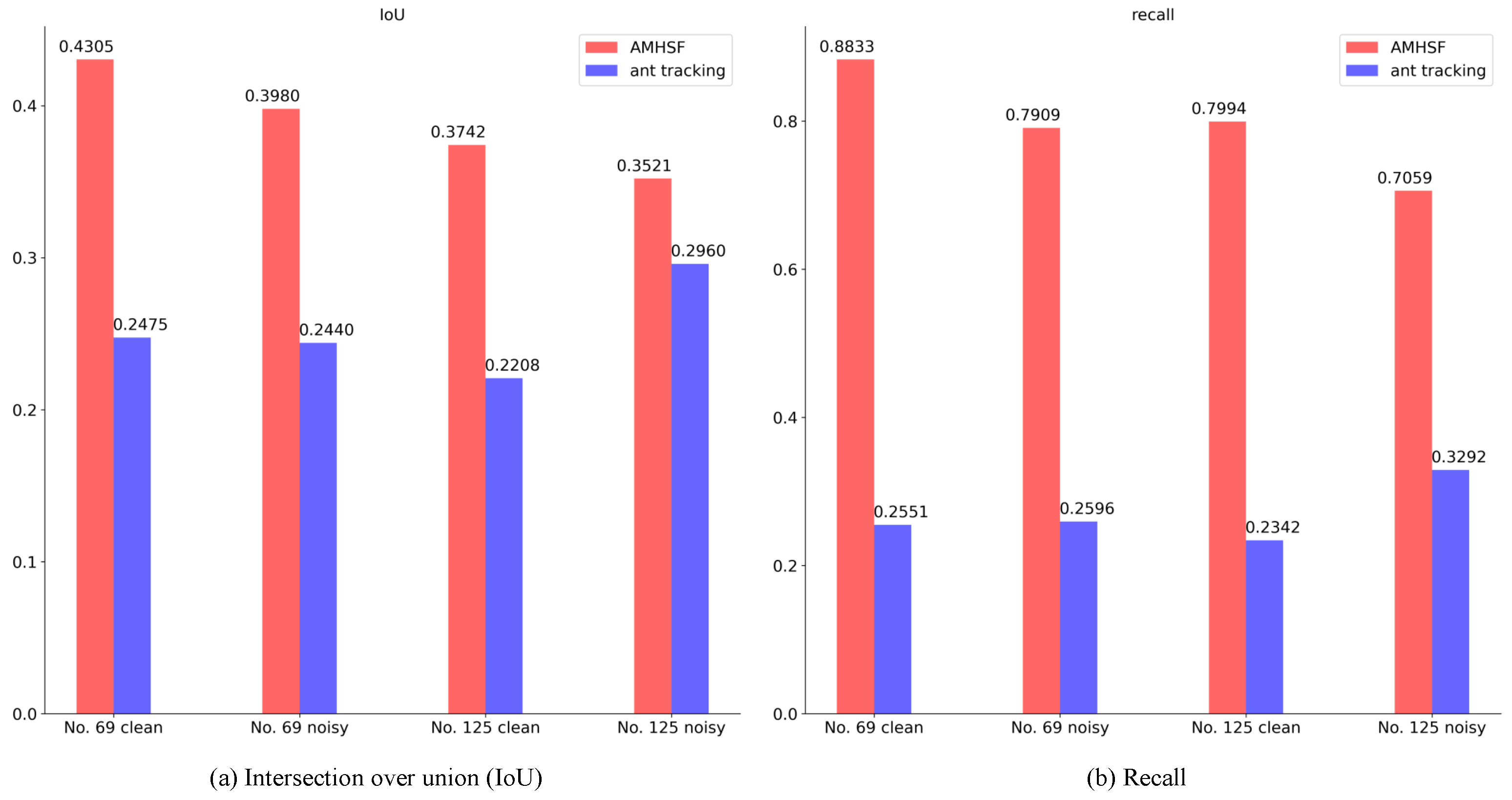
We also calculate intersection over union (IoU) and recall, two quantitative metrics commonly used in tasks such as segmentation, for evaluation and comparison. IoU measures the overall performance of a method, while recall indicates its sensitivity. The quantitative results are presented in Figure 4. Since the values of the attribute conditioning results fall within a range, we binarize the results of each method: 1 represents a fault pixel and 0 represents a non-fault pixel. Ant tracking can be binarized effortlessly by determining whether the pixel value is greater than 0. Similarly, we binarize AMHSF by modifying our refinement function:
V rfn = 1 if v > θ , 0 otherwise .
Observing Figure 4, our method outperforms ant tracking both in IoU and recall. Specifically, the recall of ant tracking is significantly lower than that of AMHSF, which validates the conclusion from visual results that ant tracking fails to extract all fault information. This limitation also negatively impacts the IoU of ant tracking. Correspondingly, our method exhibits a high recall, indicating that it has good sensitivity to sheet-like structures, i.e., the faults. Neither our method nor ant tracking achieves a high IoU, as both methods are not pixel-precision fault extraction methods, and our simplified binarization is also a bottleneck. Moreover, the introduction of Gaussian noise only leads a slight decrease in IoU, which quantitatively demonstrates the robustness of AMHSF to a level of noise. We also need to point out that we do not perform quantitative evaluation on real data because it lacks ground truth.
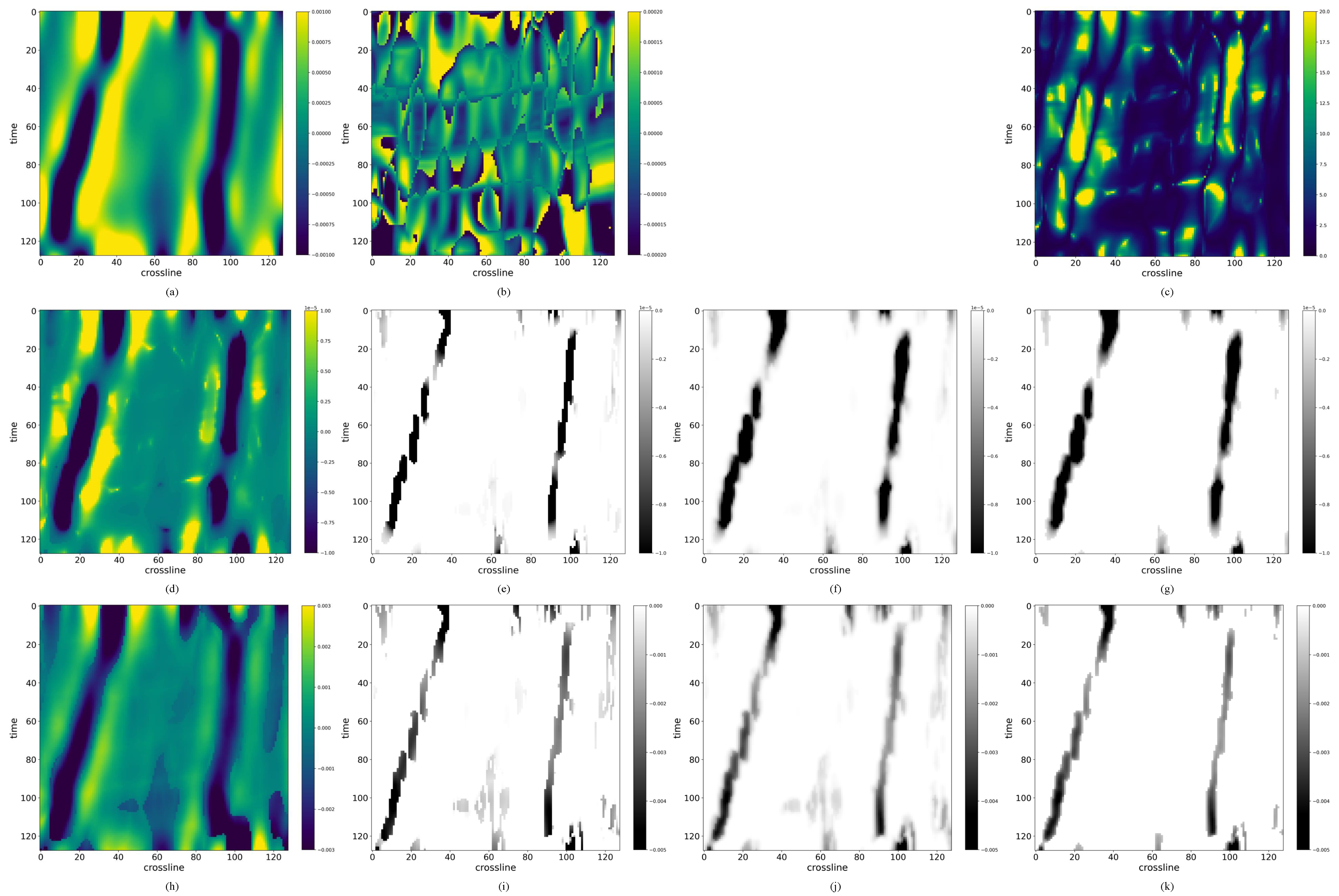
Additionally, we illustrate the intermediate results in Figure 5. To be specific, subfigure (a) depicts the 2 x 1 2 -related intermediate result from AniHessian ( · ) (line 2 of Algorithm 1), as defined in Equation (6) with parameters detailed in Table 2. Subfigure (b) is one of the eigenvalues of the anisotropic Hessian matrix, corresponding to line 3 of Algorithm 1. Subfigures (c) and (d) illustrate R sheet and V sheet , respectively, when Equation (14) is selected as our enhancement function, with subfigure (d) being the output from SheetEnhancing ( · ) (line 4 of Algorithm 1). The subsequent three subfigures ((e), (f), and (g)) present the raw attribute condition (line 6 of Algorithm 1), the diffused attribute condition (line 7 of Algorithm 1), and the final output of our method AMHSF with low-absolute-value points removed (line 8 of Algorithm 1). The intermediate results for enhancement function 15 are shown in the next four subfigures. Within them, the result given in subfigure (k) is consistent with the result in (j) of Figure 3, serving as an anchor for the impression of all the experimental results. It is worth noting that there is no R sheet to compute under this circumstance. These results clearly demonstrate that the raw attribute conditioning results (subfigures (e) and (i)) are not continuous, which is the reason we apply diffusion to smooth the raw results. Besides, both Equations (14) and (15) are effective to extract faults from coherence images, as evidenced in subfigures (e)–(g) and (i)–(k). A comparison of subfigures (f) and (j) with (g) and (k) highlights the effectiveness of the post-processing that removes the points with low absolute values in suppressing artifacts.
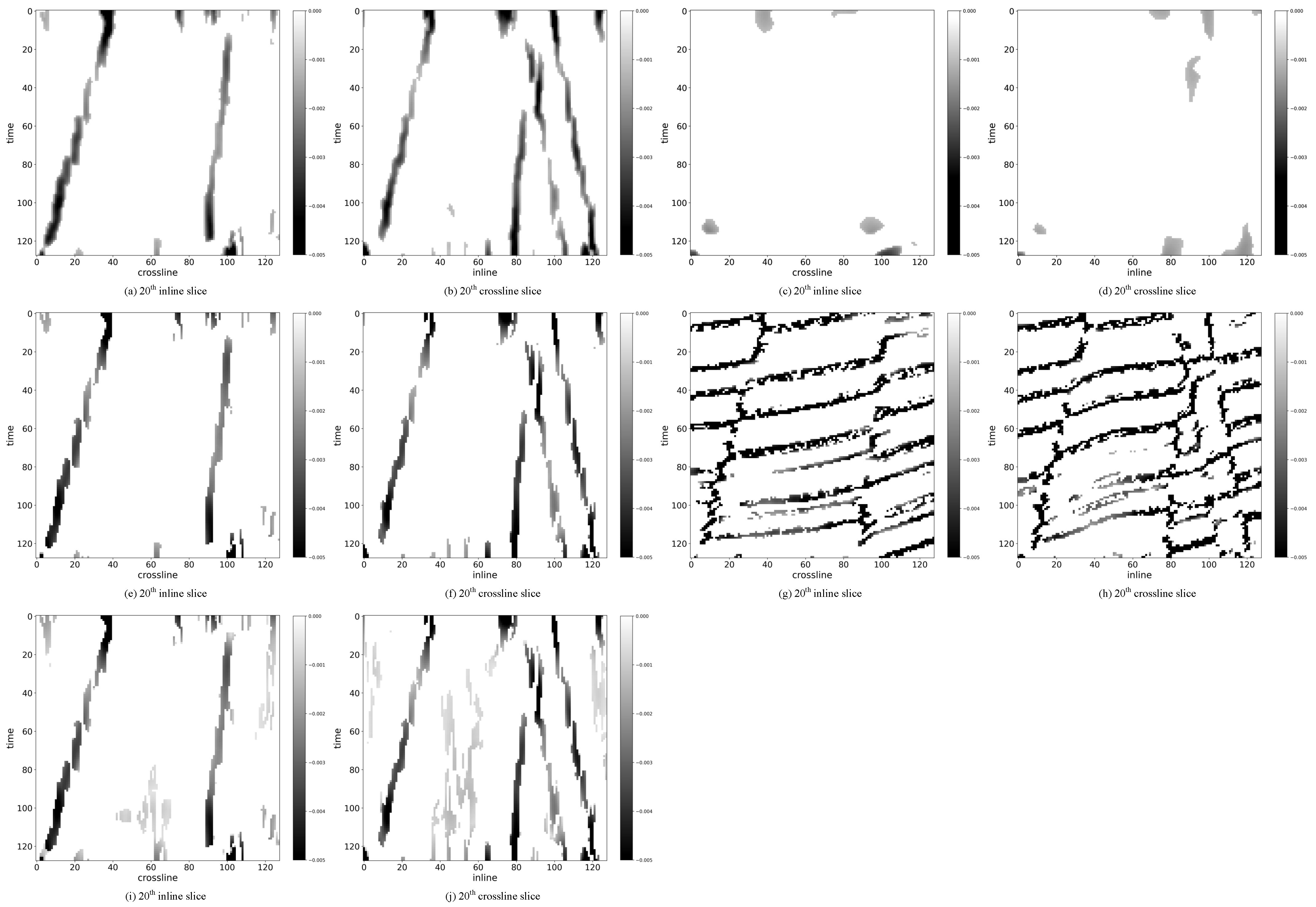
Moreover, we examine AMHSF’s sensitivity to parameters and illustrate the results in Figure 6. The subfigure (a) and subfigure (b) are the 20th inline and the 20th crossline of the No. 69 synthetic sample, respectively, corresponding to the noisy results illustrated in Figure 2. The corresponding parameters are given in Table 3, with modified configure highlighted in red. According to Figure 6, there is a minor difference when we change the values of σ c from 0.0:0.4:8.0 to 4.0:0.4:12.0. However, when we perform the same value change on σ i , the performance is severely damaged. Comparing subfigures (a), (b) with (g), (h), changing the value range of σ t will influence the appearance of horizontal stacking information, which may influence the final interpretation of the attribute conditioning output. When decreasing the threshold θ , more unwanted artifacts can be found in the results of subfigures (i) and (j), as expected. It is worth noting that this is just the straightforward description of the results. No conclusions can be drawn from the results, e.g., that σ c is less significant than σ i and that it does not impact the overall performance. In fact, the selection of parameters still needs empirical knowledge and expertise, which indicates that there exists room for improvement.

3.2. Experimental Results Using Opunake-3D

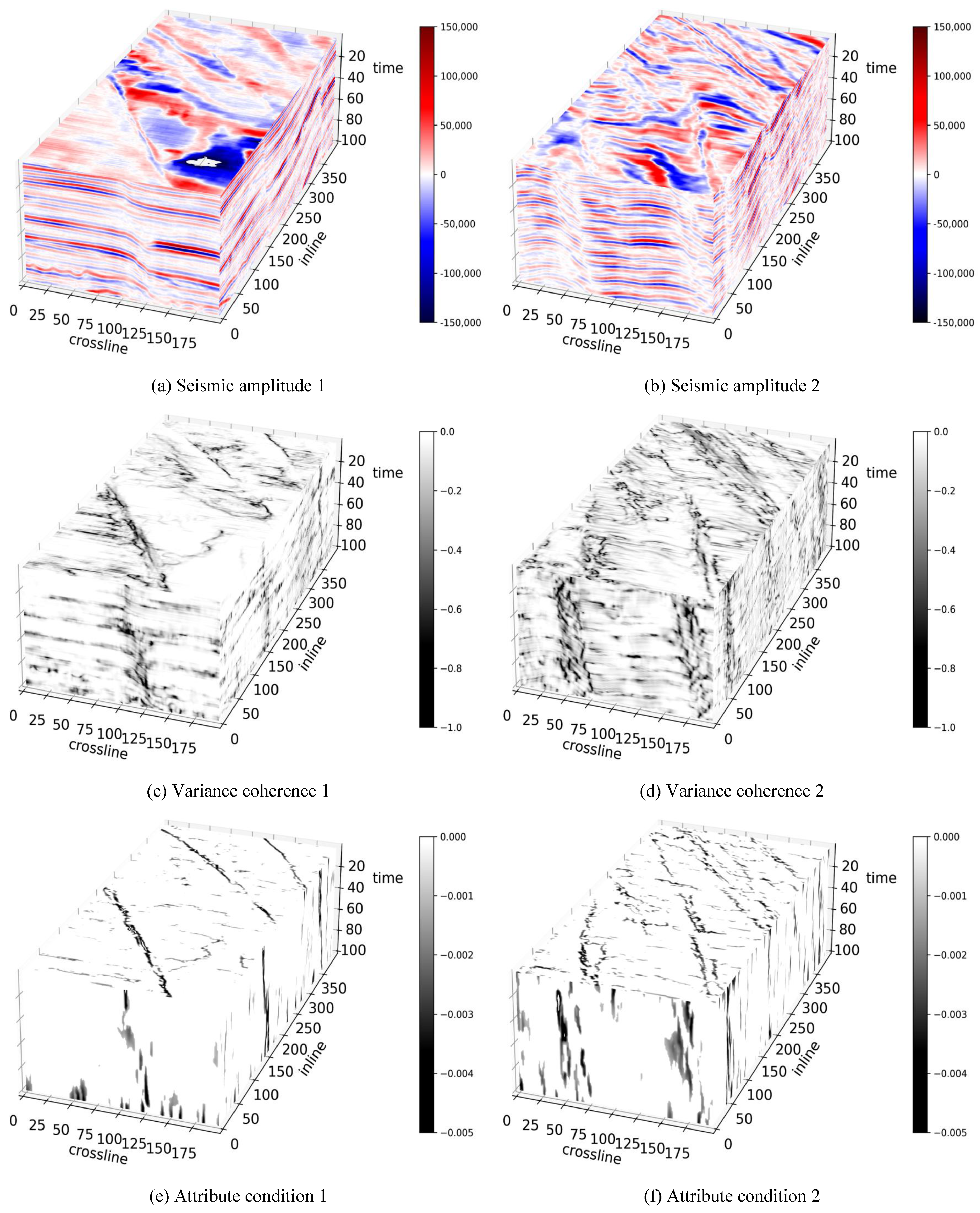
The experimental results on Opunake-3D are demonstrated in Figure 7 and Figure 8. In particular, Figure 7 presents the 3D cubes of the two randomly selected subcubes, and Figure 8 demonstrates the corresponding 50th crossline slices. As mentioned in Section 2.3, we do not add additional noise to real filed data. Subfigures (a) and (b) are the figures plotted from original seismic amplitudes, while (c) and (d) are from the variance coherence. The attribute conditions are given in subfigures (e) and (f). According to these figures, we can find that the most obvious faults in the seismic amplitudes are successfully emphasized in our attribute conditioning results, while in the coherence images, these faults are surrounded by background noise. Other less obvious discontinuities can be found in our results as well, but they are mixed with artifacts. In summary, our method is the satisfactory completion of the attribute conditioning task, but there still exists room for improvement.

3.3. Experimental Results Using Parihaka-3D

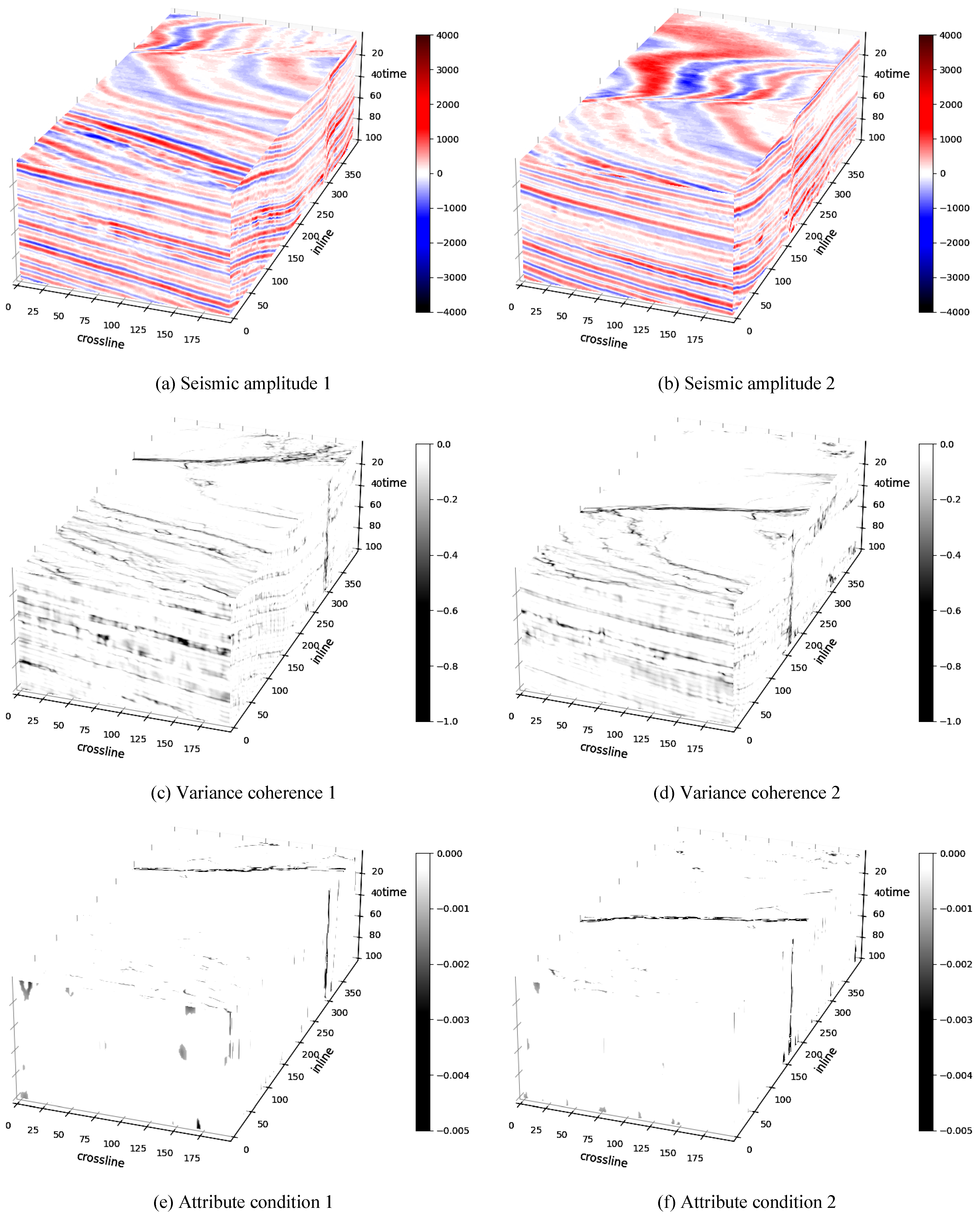
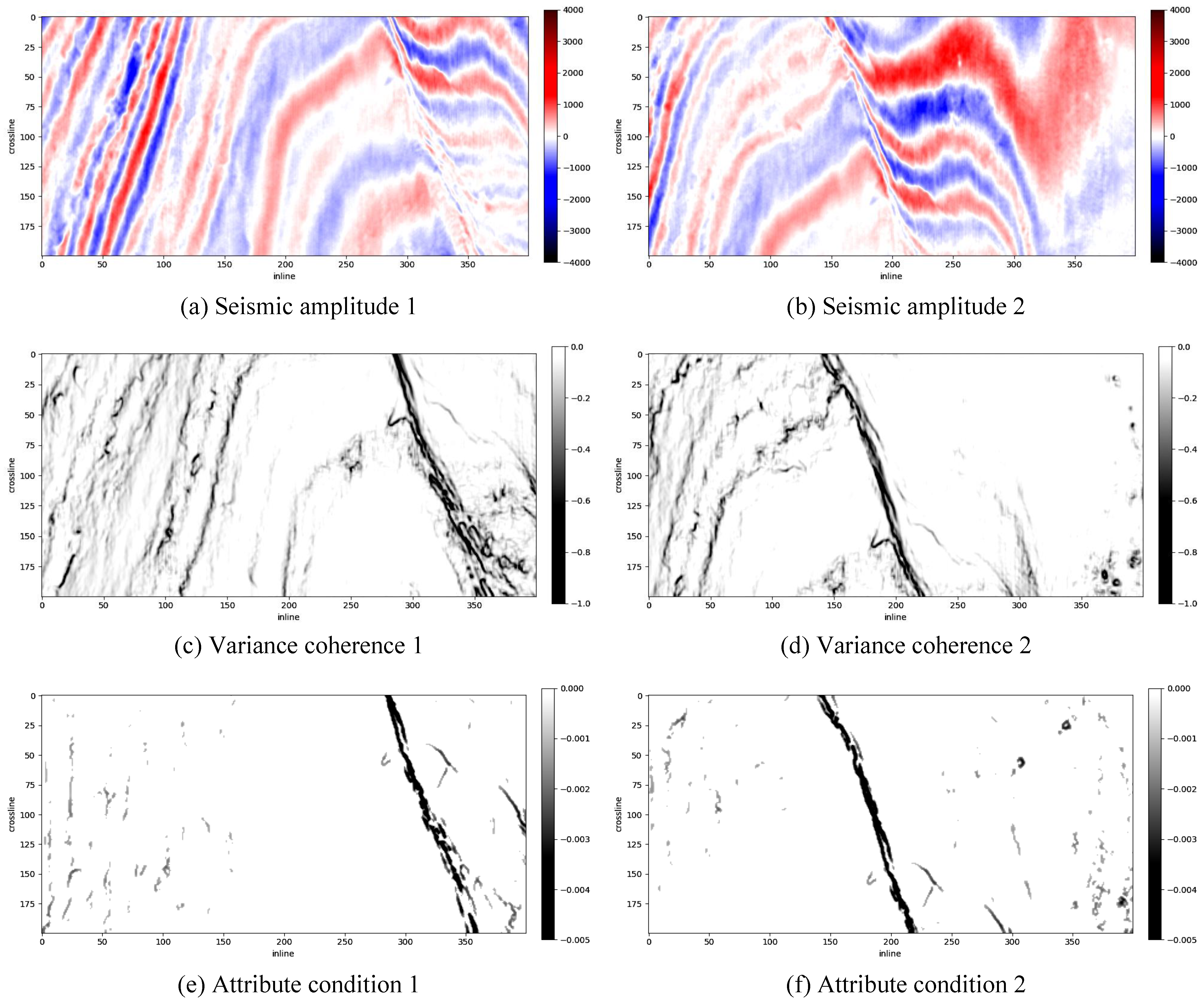
Figure 9 displays the 3D results of the experiments using Parihaka-3D and Figure 10 focuses on their 50th timeline slices. The results are shown in the same sequence as the results on Opunake-3D: the original seismic amplitudes are shown in subfigures (a) and (b), the variance coherence images are given in subfigures (c) and (d), and the outcomes of our method AMHSF, i.e., the attriobute conditions, are demonstrated in subfigures (e) and (f). Observing these results, the same conclusion as in the experiments on Opunake-3D can be reached, i.e., that our method, AMHSF, performs effectively for sheet-like structure extraction.

4. Discussion

As discussed in Section 3, our proposed AMHSF can suppress background and lateral discontinuities, revealing high-contrast faults in the results, and therefore, the sheet-like structures can be easily distinguished. Its efficacy and accuracy have already been verified on both synthetic and real field datasets. However, despite the strong geological interpretability, our method still has limitations:
(1)
Our proposed method is constructed on the fundamental assumption that seismic data exhibit sheet-like structures. This assumption is satisfied in the majority of cases of faults, as verified in [35]. While it can be readily observed that most features conform to sheet-like structures, a more comprehensive theoretical or experimental investigation is necessary to fully validate this assumption and ensure accurate attribute conditioning. When this sheet-like assumption is not satisfied, our AMHSF will also fail, which is a characteristic of modeling-based methods and a significant drawback.
(2)
Our proposed method is sensitive to the selection of parameters. Since the sheetness measure is designed to be maximal at the scale corresponding to the radius of the sheet-like structures, the sheetness index peaks near the center of these features and approaches zero outside. Therefore, to achieve optimal attribute conditioning, the scale parameters must be carefully adjusted throughout the experiment to ensure effective filtering of sheet-like structures, Also, the removal threshold requires fine-tuning, as this parameter directly impacts the suppression of unwanted artifacts in the resulting attribute images. As previously discussed, an excessively high threshold may degrade conditioning performance, while a threshold set too low may result in an excess of artifacts in the final output.
(3)
The smoothing ability of AMHSF is limited for various features, leading to difficulties in achieving continuous feature planes as [33,35]. Despite the application of smoothing for post-processing, the final results still exhibit discontinuities. However, as demonstrated in Figure 5, the attribute conditioning of the raw results is already highly effective, with faults being easily identifiable. It is highly probable that applying more advanced smoothing algorithms could lead to improved post-processing outcomes. Therefore, further exploration of smoothing techniques and their impact on the final results presents a promising direction for future work. However, still, attribute conditioning is only an intermediate step of fault detection. A more effective application may be the utilizing of our AMHSF as a pre-processing step for fault detection tasks, such as ant tracking [33], to yield more promising results.
(4)
According to other Hessian-based methods [55], the artifacts in AMHSF results may represent theoretical corner cases. As a modeling-based approach, AMHSF shares a common limitation inherent to such methods: the theoretical framework cannot encompass all possible scenarios. Although AHMSF is specifically designed for sheet-like structures, it is inevitably influenced by other non-sheet-like structures that exhibit properties similar to sheet-like structures within our method.

5. Conclusions

In this paper, we propose sheet-like structures to represent faults, with anisotropic multiscale Hessian-based sheet-enhancing filtering (AMHSF) to delineate this feature, distinguishing it from conventional attribute conditioning approaches typically employed for fault detection. A key innovation of AMHSF is the introduction of a novel enhancement function, uniquely tailored to amplify sheet-like structures, which diverges significantly from existing enhancement functions commonly used for vascular enhancement. Experimental results validate the efficacy of the AMHSF method in extracting meaningful features from coherence images compromised by significant background noise and stratigraphic discontinuities, underscoring its robustness and utility. Lastly, we believe promising directions for enhancing the performance of AMHSF include more thorough validation of the sheet-like assumption, improvements in post-processing (such as artifact removal and smoothing), and advancements in the algorithmic framework to better facilitate parameter tuning.

Author Contributions

Conceptualization, T.Z. and F.Q.; methodology, T.Z. and F.Q.; software, Y.Y. and T.C.; validation, T.Z., Y.Y. and T.C.; formal analysis, T.Z.; investigation, Y.Y. and T.C.; resources, T.Z.; data curation, T.C.; writing—original draft preparation, T.Z. and Y.Y.; writing—review and editing, T.Z. and F.Q.; visualization, T.C.; supervision, F.Q.; project administration, T.Z.; funding acquisition, F.Q. All authors have read and agreed to the published version of the manuscript.

Funding

This research was funded by the National Natural Science Foundation of China under Grant 41874155 and Grant 42130812.

Data Availability Statement

The original data presented in the study are all openly available: the synthetic 3D dataset for fault detection can be found in FaultSeg: https://github.com/xinwucwp/faultSeg (accessed on 15 January 2024), Opunake-3D is available on Seg Wiki: https://wiki.seg.org/wiki/Opunake-3D, (accessed on 5 April 2024), and Parihaka-3D is available on Seg Wiki: https://wiki.seg.org/wiki/Parihaka-3D, (accessed on 11 August 2024).

Acknowledgments

We appreciate all the contributors of FaultSeg for releasing the synthetic 3D fault dataset. We also want to thank all the contributors who collected and released the two real field datasets we used.

Conflicts of Interest

The authors declare no conflicts of interest.

Abbreviations

The following abbreviations are used in this manuscript:
MHFmultiscale Hessian-based filtering
AMHFanisotropic multiscale Hessian-based filtering
AMHSFanisotropic multiscale Hessian-based sheet-enhancing filtering

References

  1. Hesthammer, J.; Fossen, H. Research article: The influence of seismic noise in structural interpretation of seismic attribute maps. First Break 1997, 15. [Google Scholar] [CrossRef]
  2. Won, J.; Shin, J.; Ha, J.; Jun, H. Study on the seismic random noise attenuation for the seismic Attribute analysis. Econ. Environ. Geol. 2024, 57, 51–71. [Google Scholar] [CrossRef]
  3. Wen, Y.; Qian, F.; Guo, W.; Zong, J.; Peng, D.; Chen, K.; Hu, G. VSP Upgoing and Downgoing Wavefield Separation: A Hybrid Model-Data Driven Approach. IEEE Trans. Geosci. Remote Sens. 2025; in press. [Google Scholar]
  4. Wu, X.; Liang, L.; Shi, Y.; Fomel, S. FaultSeg3D: Using synthetic data sets to train an end-to-end convolutional neural network for 3D seismic fault segmentation. Geophysics 2019, 84, IM35–IM45. [Google Scholar] [CrossRef]
  5. Lin, T.; Ha, T.; Marfurt, K.J.; Deal, K.L. Quantifying the significance of coherence anomalies. Interpretation 2016, 4, T205–T213. [Google Scholar] [CrossRef]
  6. Bahorich, M.; Farmer, S. 3-D seismic discontinuity for faults and stratigraphic features: The coherence cube. Lead. Edge 1995, 14, 1053–1058. [Google Scholar] [CrossRef]
  7. Marfurt, K.J.; Kirlin, R.L.; Farmer, S.L.; Bahorich, M.S. 3-D seismic attributes using a semblance-based coherency algorithm. Geophysics 1998, 63, 1150–1165. [Google Scholar] [CrossRef]
  8. Huo, Z.; Liu, X.; Wang, X.; Chen, W. An efficient Eigenstructure-Based coherence measure via dimensionality reduction. IEEE Geosci. Remote Sens. Lett. 2019, 16, 1711–1715. [Google Scholar] [CrossRef]
  9. Sun, F.; Zhang, B. A generalized coherence algorithm based on kernel correlation. IEEE Geosci. Remote Sens. Lett. 2020, 17, 2040–2044. [Google Scholar] [CrossRef]
  10. Yang, L.; Gao, J.; Liu, N.; Yang, T.; Jiang, X. A coherence algorithm for 3-D seismic data analysis based on the mutual information. IEEE Geosci. Remote Sens. Lett. 2019, 16, 967–971. [Google Scholar] [CrossRef]
  11. Marfurt, K.J.; Sudhaker, V.; Gersztenkorn, A.; Crawford, K.D.; Nissen, S.E. Coherency calculations in the presence of structural dip. Geophysics 1999, 64, 104–111. [Google Scholar] [CrossRef]
  12. Yan, B.; Yuan, S.; Wang, S.; OuYang, Y.; Wang, T.; Shi, P. Improved eigenvalue-based coherence algorithm with dip scanning. Geophysics 2016, 82, V95–V103. [Google Scholar] [CrossRef]
  13. Rande, T.; Pedersen, S.I.; Sønneland, L. Automatic extraction of fault surfaces from three-dimensional seismic data. In SEG Technical Program Expanded Abstracts 2001; Society of Exploration Geophysicists: Houston, TX, USA, 2001; pp. 551–554. [Google Scholar] [CrossRef]
  14. Van Bemmel, P.P.; Pepper, R.E. Seismic Signal Processing Method and Apparatus for Generating a Cube of Variance Values. U.S. Patent 6,151,555, 19 August 1999. [Google Scholar]
  15. Randen, T.; Monsen, E.; Signer, C.; Abrahamsen, A.; Hansen, J.O.; Sæter, T.; Schlaf, J. Three-dimensional texture attributes for seismic data analysis. In SEG Technical Program Expanded Abstracts 2000; Society of Exploration Geophysicists: Houston, TX, USA, 2000; pp. 668–671. [Google Scholar] [CrossRef]
  16. Bakker, P. Image Structure Analysis for Seismic Interpretation. Ph.D. Thesis, Delft University of Technology, Delft, The Netherlands, 2002. [Google Scholar]
  17. Mahadik, R.; Singh, G.; Routray, A. Multispectral coherence analysis for better fault visualization in seismic data. IEEE Geosci. Remote Sens. Lett. 2022, 19, 1–5. [Google Scholar] [CrossRef]
  18. Wu, X. Directional structure-tensor-based coherence to detect seismic faults and channels. Geophysics 2017, 82, A13–A17. [Google Scholar] [CrossRef]
  19. Wang, X.; Chen, W.; Zhu, Z. Robust seismic volumetric dip estimation combining structure tensor and multiwindow technology. IEEE Trans. Geosci. Remote Sens. 2019, 57, 395–405. [Google Scholar] [CrossRef]
  20. Roberts, A. Curvature attributes and their application to 3D interpreted horizons. First Break 2001, 19, 85–100. [Google Scholar] [CrossRef]
  21. Al-Dossary, S.; Marfurt, K.J. 3D volumetric multispectral estimates of reflector curvature and rotation. Geophysics 2006, 71, P41–P51. [Google Scholar] [CrossRef]
  22. Ao, Y.; Lu, W.; Jiang, B.; Monkam, P. Seismic structural curvature volume extraction with convolutional neural networks. IEEE Trans. Geosci. Remote Sens. 2021, 59, 7370–7384. [Google Scholar] [CrossRef]
  23. Gao, D. Integrating 3D seismic curvature and curvature gradient attributes for fracture characterization: Methodologies and interpretational implications. Geophysics 2013, 78, O21–O31. [Google Scholar] [CrossRef]
  24. Klein, P.; Richard, L.; James, H. 3D curvature attributes: A new approach for seismic interpretation. First Break 2008, 26. [Google Scholar] [CrossRef]
  25. Qi, X.; Marfurt, K. Volumetric aberrancy to map subtle faults and flexures. Interpretation 2018, 6, T349–T365. [Google Scholar] [CrossRef]
  26. Lyu, B.; Qi, J.; Li, F.; Marfurt, K.J. Multispectral aberrancy. In SEG Technical Program Expanded Abstracts 2020; Society of Exploration Geophysicists: Houston, TX, USA, 2020; pp. 1120–1124. [Google Scholar] [CrossRef]
  27. Hale, D. Methods to compute fault images, extract fault surfaces, and estimate fault throws from 3D seismic images. Geophysics 2013, 78, O33–O43. [Google Scholar] [CrossRef]
  28. Qi, J.; Lyu, B.; AlAli, A.; Machado, G.; Hu, Y.; Marfurt, K. Image processing of seismic attributes for automatic fault extraction. Geophysics 2019, 84, O25–O37. [Google Scholar] [CrossRef]
  29. Neff, D.B.; Grismore, J.R.; Lucas, W.A. Automated Seismic Fault Detection and Picking. U.S. Patent 6,018,498, 2 September 1998. [Google Scholar]
  30. Cohen, I.; Coult, N.; Vassiliou, A.A. Detection and extraction of fault surfaces in 3D seismic data. Geophysics 2006, 71, P21–P27. [Google Scholar] [CrossRef]
  31. Wu, X.; Hale, D. 3D seismic image processing for faults. Geophysics 2016, 81, IM1–IM11. [Google Scholar] [CrossRef]
  32. Wu, X.; Zhu, Z. Methods to enhance seismic faults and construct fault surfaces. Comput. Geosci. 2017, 107, 37–48. [Google Scholar] [CrossRef]
  33. Pedersen, S.I.; Randen, T.; Sønneland, L.; Steen, Ø. Automatic fault extraction using artificial ants. In SEG Technical Program Expanded Abstracts 2002; Society of Exploration Geophysicists: Houston, TX, USA, 2002; pp. 512–515. [Google Scholar] [CrossRef]
  34. Han, J.; Gu, B.; Zhu, G.; Liu, Z. High-Precision Depth Domain Migration Method in Imaging of 3D Seismic Data in Coalfield. Remote Sens. 2022, 14, 2850. [Google Scholar] [CrossRef]
  35. Wu, X.; Fomel, S. Automatic fault interpretation with optimal surface voting. Geophysics 2018, 83, O67–O82. [Google Scholar] [CrossRef]
  36. Huang, L.; Dong, X.; Clee, T.E. A scalable deep learning platform for identifying geologic features from seismic attributes. Lead. Edge 2017, 36, 249–256. [Google Scholar] [CrossRef]
  37. Xiong, W.; Ji, X.; Ma, Y.; Wang, Y.; AlBinHassan, N.M.; Ali, M.N.; Luo, Y. Seismic fault detection with convolutional neural network. Geophysics 2018, 83, O97–O103. [Google Scholar] [CrossRef]
  38. Hu, G.; Hu, Z.; Liu, J.; Cheng, F.; Peng, D. Seismic fault interpretation using Deep Learning-Based Semantic Segmentation Method. IEEE Geosci. Remote Sens. Lett. 2020, 19, 1–5. [Google Scholar] [CrossRef]
  39. Wang, Z.; Li, B.; Liu, N.; Wu, B.; Zhu, X. Distilling knowledge from an ensemble of convolutional neural networks for seismic fault detection. IEEE Geosci. Remote Sens. Lett. 2020, 19, 1–5. [Google Scholar] [CrossRef]
  40. Pochet, A.; Diniz, P.H.B.; Lopes, H.; Gattass, M. Seismic fault detection using convolutional neural networks trained on synthetic poststacked amplitude maps. IEEE Geosci. Remote Sens. Lett. 2018, 16, 352–356. [Google Scholar] [CrossRef]
  41. Tang, Z.; Wu, B.; Wu, W.; Ma, D. Fault Detection via 2.5D Transformer U-Net with Seismic Data Pre-Processing. Remote Sens. 2023, 15, 1039. [Google Scholar] [CrossRef]
  42. Zhang, Z.; Chen, R.; Ma, J. Improving Seismic Fault Recognition with Self-Supervised Pre-Training: A Study of 3D Transformer-Based with Multi-Scale Decoding and Fusion. Remote Sens. 2024, 16, 922. [Google Scholar] [CrossRef]
  43. Frangi, A.F.; Niessen, W.J.; Vincken, K.L.; Viergever, M.A. Multiscale vessel enhancement filtering. In Proceedings of the Medical Image Computing and Computer-Assisted Intervention, Cambridge, MA, USA, 11–33 October 1998. [Google Scholar]
  44. Annunziata, R.; Garzelli, A.; Ballerini, L.; Mecocci, A.; Trucco, E. Leveraging multiscale Hessian-Based enhancement with a novel exudate inpainting technique for retinal vessel segmentation. IEEE J. Biomed. Health Inform. 2015, 20, 1129–1138. [Google Scholar] [CrossRef]
  45. Jerman, T.; Pernus, F.; Likar, B.; Spiclin, Z. Enhancement of vascular structures in 3D and 2D angiographic images. IEEE Trans. Med. Imaging 2016, 35, 2107–2118. [Google Scholar] [CrossRef]
  46. Descoteaux, M.; Audette, M.; Chinzei, K.; Siddiqi, K. Bone enhancement filtering: Application to sinus bone segmentation and simulation of pituitary surgery. Comput. Aided Surg. 2006, 11, 247–255. [Google Scholar] [CrossRef]
  47. Geusebroek, J.; Smeulders, A.W.M.; Van De Weijer, J. Fast anisotropic gauss filtering. IEEE Trans. Image Process. 2003, 12, 938–943. [Google Scholar] [CrossRef]
  48. Nie, S.; Yu, J.; Chen, P.; Wang, Y.; Zhang, J.Q. A Hessian plate filter and shape feature-based approach to automatically localizing the NT VOI of 3D ultrasound data. Comput. Assist. Surg. 2016, 21 (Suppl. S1), 83–91. [Google Scholar] [CrossRef]
  49. Voorn, M.; Exner, U.; Rath, A. Multiscale Hessian fracture filtering for the enhancement and segmentation of narrow fractures in 3D image data. Comput. Geosci. 2013, 57, 44–53. [Google Scholar] [CrossRef]
  50. Sato, Y.; Westin, C.; Bhalerao, A.; Nakajima, S.; Shiraga, N.; Tamura, S.; Kikinis, R. Tissue classification based on 3D local intensity structures for volume rendering. IEEE Trans. Vis. Comput. Graph. 2000, 6, 160–180. [Google Scholar] [CrossRef]
  51. Charalampidis, D. Recursive implementation of the Gaussian filter using truncated cosine functions. IEEE Trans. Signal Process. 2016, 64, 3554–3565. [Google Scholar] [CrossRef]
  52. Hale, D. Recursive Gaussian filters. Tech. Rep. CWP-546, Center for Wave Phenomena, Colorado School of Mines, Golden. Colorado. 2006. Available online: https://cwp.mines.edu/wp-content/uploads/sites/112/2018/09/cwp546.pdf (accessed on 4 December 2024).
  53. Kopp, J. Efficient numerical diagonalization of hermitian 3 × 3 matrices. Int. J. Mod. Phys. C 2008, 19, 523–548. [Google Scholar] [CrossRef]
  54. Weickert, J. Anisotropic Diffusion in Image Processing; Teubner: Stuttgart, Germany, 1998. [Google Scholar]
  55. Vignati, A.; Giannini, V.; Bert, A.; Borrelli, P.; De Luca, M.; Martincich, L.; Sardanelli, F.; Regge, D. A fully automatic multiscale 3-Dimensional Hessian-Based algorithm for vessel detection in breast DCE-MRI. Investig. Radiol. 2012, 47, 705–710. [Google Scholar] [CrossRef]
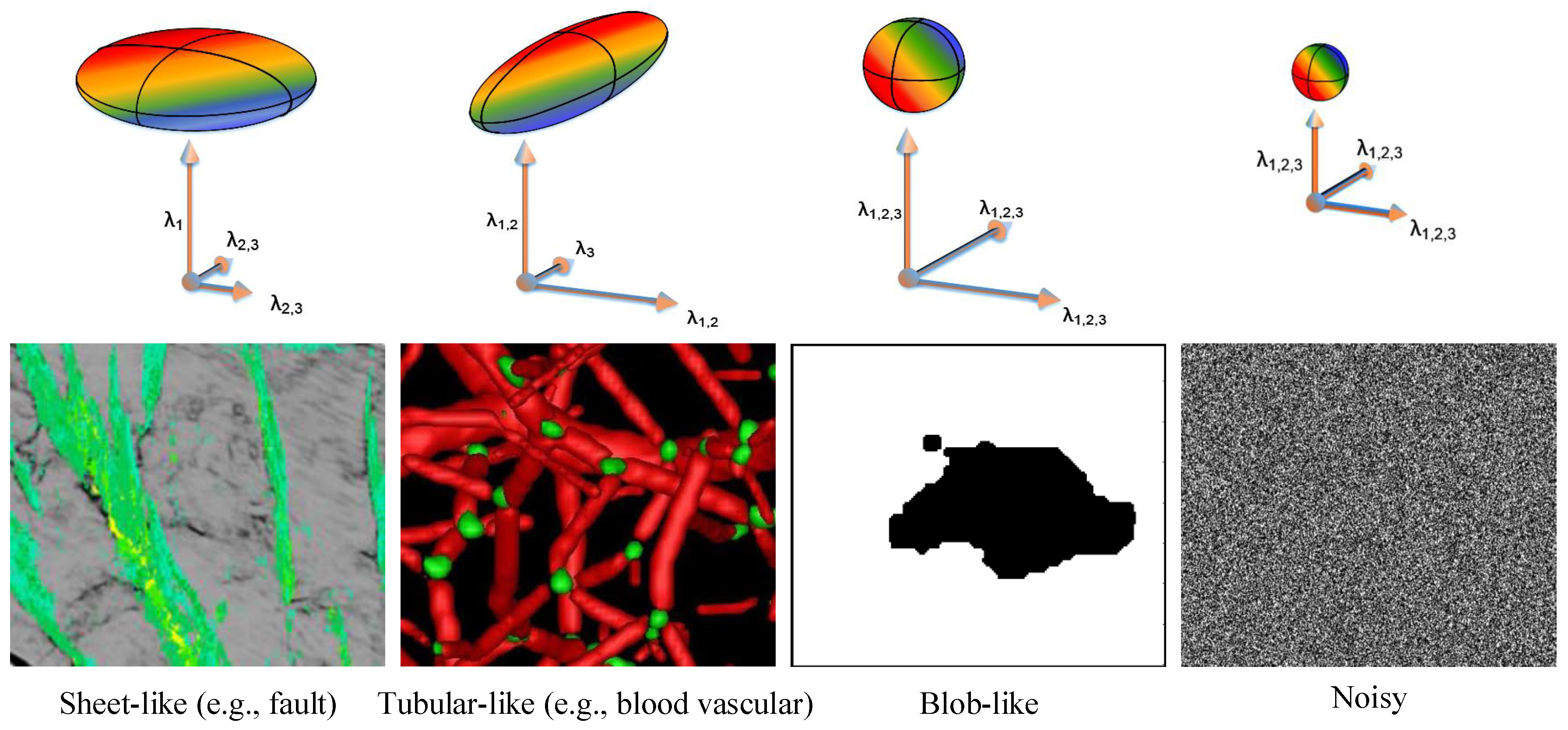
Figure 1. The relation between the eigenvalues of the Hessian matrix and image structure orientations, including a sheet, a tube, a blob, and noise. Note that our interpretation features have sheet-like structures, while the vascular features fuse tubular structures.
Remotesensing 17 00278 g001
Figure 2. The 3D cubes of attribute conditioning results on the synthetic 3D fault dataset. (ad) Seismic amplitudes, (eh) variance coherence, (il) attribute condition (results) obtained by AMHSF, (mp) attribute condition (results) obtained by ant tracking, and (q,r) the ground truth faults.
Remotesensing 17 00278 g002
Figure 3. The effect of the 20th inline slices of attribute conditioning results on the synthetic 3D fault dataset. (ad) Seismic amplitudes, (eh) variance coherence, (il) attribute condition (results) obtained by AMHSF, (mp) attribute condition (results) obtained by ant tracking, and (q,r) the ground truth faults.
Remotesensing 17 00278 g003
Figure 4. The quantitative comparison of the results between our AMHSF and ant tracking.
Remotesensing 17 00278 g004
Figure 5. The intermediate attribute conditioning results on the synthetic 3D fault dataset. (a) Anisotropic Hessian, (b) eigenvalue, (cg) intermediate results using Equation (14), and (hk) intermediate results using Equation (15).
Remotesensing 17 00278 g005
Figure 6. The impact of parameter selection. Corresponding parameters are given in Table 3.
Remotesensing 17 00278 g006
Figure 7. The 3D cubes of attribute conditioning results using Opunake-3D.
Remotesensing 17 00278 g007
Figure 8. The 50th crossline slices of attribute conditioning results using Opunake-3D.
Remotesensing 17 00278 g008
Figure 9. The 3D cubes of attribute conditioning results using Parihaka-3D.
Remotesensing 17 00278 g009
Figure 10. The 50th timeline slices of attribute conditioning results using Parihaka-3D.
Remotesensing 17 00278 g010
Table 1. The relation between the eigenvalues of the Hessian matrix and image structure orientation.
 Structure Type   λ 1 *  λ 2 *  λ 3 *
Sheet-like, brightLowLowHigh negative
Sheet-like, darkLowLowHigh positive
Tubular-like, brightLowHigh negativeHigh negative
Tubular-like, darkLowHigh positiveHigh positive
Blob-like, brightHigh negativeHigh negativeHigh negative
Blob-like, darkHigh positiveHigh positiveHigh positive
NoisyLowLowLow
* As mentioned earlier, λ 1 , λ 2 , and λ 3 correspond to the eigenvalues along the inline, crossline, and timeline, respectively.
Table 2. Parameter settings.
Dataset σ i σ c σ t θ
Synthetic0.0:0.4:8.0 *0.0:0.4:8.00.0:0.15:3.0 0.0015
Opunake-3D0.0:0.2:4.00.0:0.2:4.04.0:0.2:8.0 0.001
Parihaka-3D0.0:0.1:4.00.0:0.1:4.02.0:0.1:6.0 0.001
* 0.0:0.4:8.0 is the Matlab notation for 0.0 σ i 8.0 with interval 0.4 , the rest are likewise.
Table 3. Corresponding parameters of results in Figure 6.
  σ i σ c σ t θ
Figure 5a *0.0:0.4:8.00.0:0.4:8.00.0:0.15:3.00.0015
Figure 5b *0.0:0.4:8.00.0:0.4:8.00.0:0.15:3.00.0015
Figure 5c4.0:0.4:12.00.0:0.4:8.00.0:0.15:3.00.0015
Figure 5d4.0:0.4:12.00.0:0.4:8.00.0:0.15:3.00.0015
Figure 5e0.0:0.4:8.04.0:0.4:12.00.0:0.15:3.00.0015
Figure 5f0.0:0.4:8.04.0:0.4:12.00.0:0.15:3.00.0015
Figure 5g0.0:0.4:8.00.0:0.4:8.00.0:0.05:1.00.0015
Figure 5h0.0:0.4:8.00.0:0.4:8.00.0:0.05:1.00.0015
Figure 5i0.0:0.4:8.00.0:0.4:8.00.0:0.15:3.00.0005
Figure 5j0.0:0.4:8.00.0:0.4:8.00.0:0.15:3.00.0005
* These results have the same parameters as those used in Figure 2 and Figure 4.
Disclaimer/Publisher’s Note: The statements, opinions and data contained in all publications are solely those of the individual author(s) and contributor(s) and not of MDPI and/or the editor(s). MDPI and/or the editor(s) disclaim responsibility for any injury to people or property resulting from any ideas, methods, instructions or products referred to in the content.