Abstract
In the process of airborne radar imaging, when encountering certain scenarios (e.g., the Gobi desert), the low number or absence of strong scattering points will lead to azimuth scattering in the imaging results. In this study, we propose an autofocusing method based on the traditional phase gradient autofocus (PGA) algorithm that determines the optimal number of strong scattering points in each azimuth sub-aperture according to the scene (i.e., adaptively) and uses the mean amplitudes of these points in each azimuth sub-aperture of the scene to make a threshold judgment. In this way, the optimal number of strong scattering points is iteratively selected for subsequent PGA processing. The focusing quality of the image is significantly improved through the combination of these algorithms with onboard radar imaging. The simulation results prove the effectiveness of the method proposed in this study, compared with traditional PGA.
1. Introduction
Radar imaging technology originated in the 1950s and is a landmark invention in the field of radar technology [1]. Compared with optical imaging systems, imaging radar has no light condition requirements and can work 24 h a day; as such, it is of particular use in the field of military intelligence.
At present, synthetic aperture radar (SAR) [2] is the most widely used radar imaging technology, which is a high-resolution imaging radar utilizing small antennas that move along a long array trajectory while emitting phase-referenced signals and coherently processing the echo signals from different locations. The imaging regime of SAR is expected to be extended and expanded in the future, in terms of its observation dimensions, in order to obtain multi-dimensional information about targets [3,4,5]. In SAR imaging, when the radar system acquires two-dimensional SAR images under different flight paths through repeated observations [6,7,8,9], the phase error caused by the transmission of echo signals can lead to image defocusing, affecting the quality of the resulting SAR images. With the improvement of imaging resolution, the effect of echo phase error on image defocusing is becoming more and more serious. Although navigation motion compensation systems can compensate for this phase error, to a certain extent, the residual phase error will still lead to scattering in high-resolution images. Therefore, in high-resolution SAR imaging systems, in addition to motion compensation using inertial guidance data, it is usually necessary to automatically estimate and compensate for the residual phase error of SAR echo data. This process is called autofocusing.
Autofocusing techniques based on echo data error correction have been a research hotspots for phase error correction. In this line, one class of methods utilizes autofocusing techniques based on sharpness optimization. Such methods measure the focusing quality through evaluating the sharpness of images and estimate the phase error through iteratively optimizing the sharpness function. Commonly used sharpness evaluation criteria include entropy and contrast, among others. In 2012, Pardini et al. [10] proposed a method to improve the imaging quality through minimizing the entropy of the inverse profile; however, this method suffers from the problem of bias. In 2018, Aghababaee et al. [11] introduced phase-gradient constraints in order to overcome this problem. However, this method requires multi-dimensional optimization for each pixel, leading to high computational burdens. In 2020, Feng Dong of the National University of Defense Technology proposed a sharpness-optimized autofocusing method based on intensity-squared maximization [12], which yielded similar results to the study mentioned above [11] in terms of imaging quality, while presenting advantages in terms of computational efficiency.
Another class of autofocus algorithms is based on the phase error function, the main representative of which is the phase gradient autofocus (PGA) method [13]. This method is characterized by the direct estimation of the phase error in the echo signal without the need to model the phase error. Compared with traditional autofocusing algorithms, such as map drift (MD) and phase difference (PD) [14,15,16], the PGA imposes no limitations on the phase error order and can basically adapt to strip and cluster SAR imaging contexts for various scenes. Therefore, the PGA algorithm has been widely used in the field of SAR imaging since its proposal in the 1990s, and as one of the most commonly used autofocusing algorithms, it has attracted great attention in the international SAR imaging field. This algorithm, which abandons the finite-order phase model, is a purely data-driven method providing faster convergence speed and good robustness, and it can provide good compensation for any order phase error, which makes up for the shortcomings of early autofocusing techniques in compensating for the high-order phase error. The traditional PGA algorithm was first proposed for the clustered-beam SAR imaging mode, which is suitable for radar imaging of small scenes [17]. However, when the PGA algorithm is applied for SAR imaging of large scenes, two problems arise: first, there may be multiple strong scattering centers in the same distance cell in some scenes, which is not conducive to fully extracting the scene phase error; second, in the strip imaging mode, the antenna beam slides along a fixed trajectory at a plateau velocity, and the spatial positions of various scatterers corresponding to the synthetic aperture vary according to their positions with respect to the trajectory. In other words, the SAR imaging system yields different phase errors for scatterers at different spatial locations, and the variation in these phase errors leads to the defocusing of large scenes.
In 1998, Chan proposed the QPGA method [18], which does not require iteration and only filters the strong scattering points selected in the PGA. Compared with traditional PGA processing, this method demonstrated a substantial reduction in computation and improves the focusing effect, constituting a good improvement for the development of PGA. In 1999, Thompson and Bates presented a PGA extension method based on phase-weighted estimation, which takes into account the variation in the phase error at low observation angles, at the National Radar Conference organized by the IEEE Electrical and Electronics Engineering Society. Using a weighting method to compensate for different spatial positions to different degrees can effectively improve the focusing performance in SAR imaging; however, the huge amount of computation affects the practical value of the method [19]. In the same year, Wei Ye of Xidian University (XDU), Xi’an, China) proposed a method for phase error estimation using weighted least-squares (WLSs) [20], which does not require each distance cell in the image to have its own distribution model and presents strong robustness. Zhu Zhaoda and Wu Xinwei from Nanjing University of Aeronautics and Astronautics (NUAA, Nanjing, China) extended the PGA algorithm in 2002; in particular, they utilized the intrinsic connection between the strip and cluster modes and processed the strip-mode imaging data in chunks, where each piece of the data has a certain overlap, and the phase error can be roughly regarded as a non-null-variable, such that the strip-mode data are considered equivalent to the cluster-mode data [21]. Then, image processing is carried out using the irradiation method of cluster-beam SAR, and the autofocusing process for each piece of data is completed using PGA. Finally, each of the data sub-images is spliced together, thus realizing the chunked PGA processing method of strip SAR. In 2011, Sun Xilong of the National University of Defense Technology (NUDT, Changsha, China) combined the idea of the least squares method [22] and proposed an improved PGA phase error compensation method to estimate the clutter variance based on the characteristics of the clutter energy in the extrapolated unit. This method has better applicability, due to the infinite qualitative assumption for clutter. A two-dimensional autofocusing algorithm for SAR based on a priori knowledge was proposed by Xinhua Mao and Ocean Cao of NUAA in 2013 in Electronics Letters [23]. They considered the scattering of SAR images at different distance units and analyzed the structure of the residual error handled by the SAR imaging algorithm, allowing for determination of the internal coupling problem between the distance and orientation errors. This helped them to develop a two-dimensional PGA algorithm with a better focusing effect than the existing one-dimensional PGA. In 2016, Zhang Lei et al. at XUET proposed an improved sub-aperture projection (SATA) algorithm [24,25], which corrects the azimuth phase error by calculating the phase error within each sub-aperture. In 2019, Feng et al. [26] applied the PGA method to the Holo SAR system in order to correct the phase error between different channels. It should be noted that the assumption for the PGA method that the spatial variation in phase error can be ignored may not hold in large scenarios, thus limiting its effectiveness in large-scale applications. In order to solve the phase error correction problem in large scenes, in 2021, Lu et al. [27] proposed a PGA method based on persistent scatterer (PS) point network construction (NC), which draws on the idea of a PS point network in PS-interferometric SAR (InSAR). The NC-PGA method processes the imaging scene in chunks and uses the PGA method to estimate the phase errors in subchunks. In each sub-block, the PS-point network is used to estimate the PS-point heights, thus avoiding the height offset problem between sub-blocks. In 2022, Lu et al. [28] optimized the network structure of NC-PGA. Their method uses a partially overlapping PS-point network, which significantly reduces the computational burden.
In the existing PGA algorithms, phase gradient estimation is required to estimate the phase difference based on the strong scattering points of the scene in the two-dimensional data domain. However, in some special scenes—such as the Gobi Desert and certain other scenes—with insufficient or a lack of strong scattering points, when the strong scattering points are selected for phase error estimation, the low signal-to-noise ratio of the samples of the strong scattering points leads to inaccurate estimation of the phase error, which, thus, leads to azimuth-scattered focus. In order to solve this problem, this study proposes an adaptive strong scattering-point selection method based on the mean value of the scene. The novelty of this method is that it improves the robustness of the PGA, and the radar can focus well within different scenes.
2. Materials and Methods
2.1. Introduction to PGA Algorithm
An SAR is a two-dimensional high-resolution imaging system based on digital signal technology. It is a further extension of the traditional radar concept, which significantly improves the coverage and imaging accuracy of scene targets (e.g., rivers, mountains, buildings, armored vehicles, and tanks) and which has been widely used in both military and civilian applications as it can provide more and richer information. As radar is based on electromagnetic waves, SAR imaging is not affected by light and climate conditions. SAR imaging technology is a key focus of research in the field of radar imaging.
SAR imaging systems can be divided into airborne, bomb-carrying, and star-carrying SAR imaging systems; in particular, the PGA technology considered in this study is based on airborne SAR imaging systems.
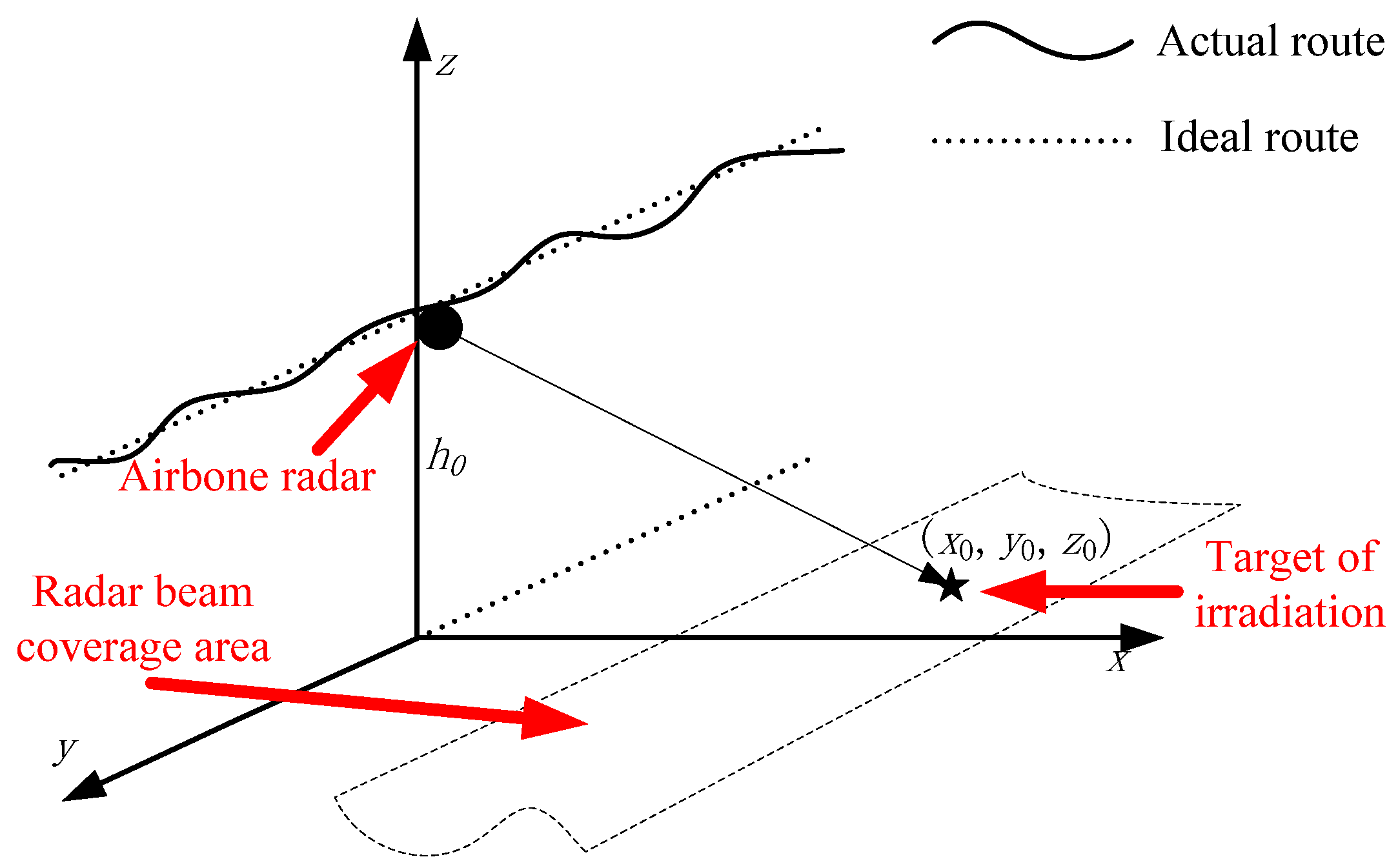
Figure 1 shows the geometric model of airborne SAR imaging, which can cause problems such as high-frequency phase errors due to electromagnetic wave propagation, carrier platform jitter, and other factors. This leads to problems such as image scattering, geometric distortion, and a low image signal-to-noise ratio. Therefore, to obtain high-resolution images, the image must be processed using a PGA-based approach.

Figure 1.
Geometric model of airborne synthetic aperture radar (SAR) imaging.
Usually, motion compensation for SAR imaging can be performed utilizing platform motion data provided by the inertial guidance system [29]. However, when the motion accuracy requirement exceeds the accuracy limit of the inertial guidance system, the radar’s Doppler phase history parameter error cannot be precisely controlled. Thus, radar imaging quality cannot be guaranteed. Therefore, it is necessary to focus the radar based on its real-time echo data, namely, using an autofocusing technique.
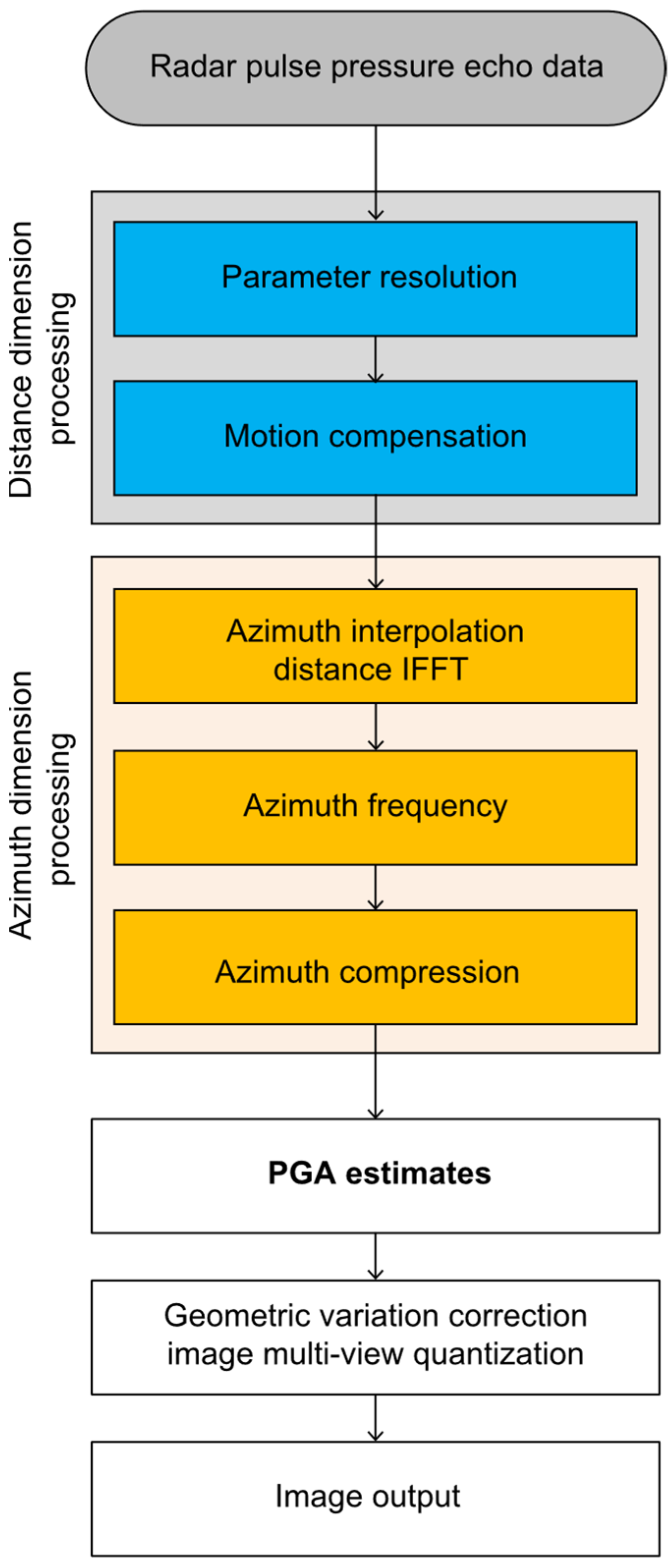
The two most commonly used autofocusing algorithms are PGA and sub-aperture correlation map drift (MD). The MD algorithm can only estimate the low-level phase error of the scene, which makes it difficult to apply in the context of high-resolution imaging. The PGA algorithm discards the finite-order phase error model and directly estimates the phase error [30], meaning that can be applied to a phase error of any order and is also applicable to various scenes in cluster mode [31] for imaging. The PGA algorithm and other algorithms for SAR imaging processing are independent of each other, and this algorithm has been widely used as a mainstream autofocusing algorithm in the field of SAR imaging. Figure 2 details the application of the PGA algorithm in an SAR display system.
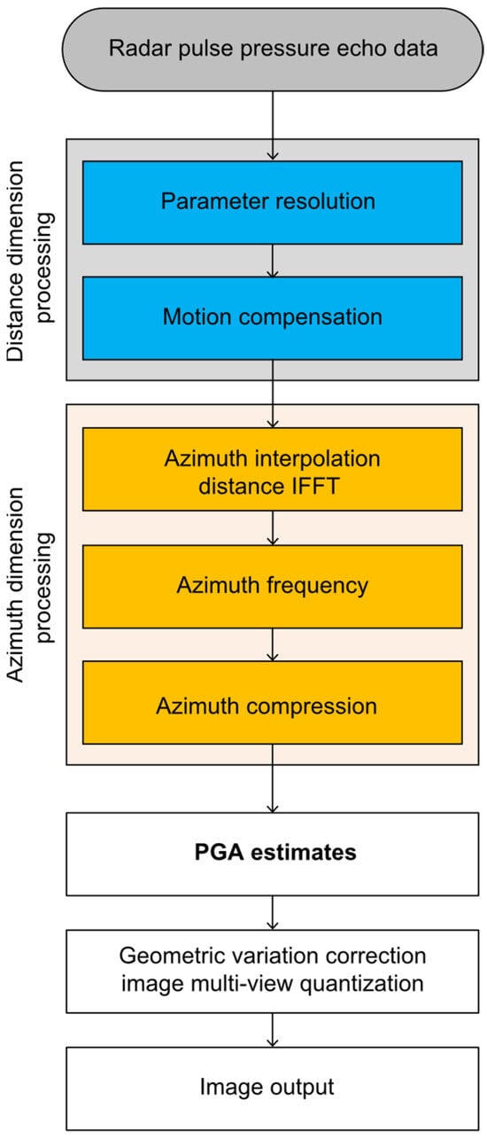
Figure 2.
Flowchart of SAR imaging based on phase gradient autofocus (PGA) processing. IFFT, inverse fast Fourier transform.
PGA was originally proposed based on cluster-beam SAR imaging. In cluster-beam SAR imaging, the complex image data and the phase history of each point in the data are related as Fourier transform pairs, where the phase history of any point covers the entire azimuth phase error. In strip SAR imaging, the phase history of a point target is acquired through the inverse process of azimuth dimensional imaging, and there is two-dimensional variability in the phase error [32]. The specific process of applying PGA to strip SAR imaging is as follows. First, the strong amplitude scattering points in the strip SAR image are selected. Second, the location of each strong scattering point is taken as a center. Third, the strong amplitude scattering points are added to a window and used to perform the convolution operation with the reference linear frequency modulation (FM) signal, in order to recover the data before the azimuth pulse pressure [33]. Fourth, a synthetic aperture strip is intercepted with the data centered on the original position of the point target, in order to solve the line frequency tuning pulse pressure before the gradient of the phase error is estimated, according to the standard PGA algorithm flow. Finally, the phase error of the whole image is obtained by splicing the gradient of the phase error of each point [34]. The specific process is as follows:
- Chunking:
Assuming that the distance-to-variance ratio over the entire image data is negligible, the image data are chunked into azimuth sub-apertures. The azimuth variance within each azimuth sub-aperture must be negligible.
- 2.
- Selection of points:
Isolated strong scattering points are selected in each azimuth sub-aperture. These points have a strong signal-to-noise ratio and can help us to estimate the phase error more accurately. The selected isolated strong scattering point is used as the center before adding a window and the reference linear FM signal for convolution. This process is carried out to recover the data before image orientation and compression; at this time, the phase error model of the point target is
where represents the azimuth time-domain coordinate, represents the echo signal at the strong scattering point, represents the phase error, and is the point-target initial phase.
- 3.
- Round shift:
The frequency-domain point pulse data are round-shifted to zero frequency, in order to remove the primary term in the phase.
- 4.
- Windowing:
In order to remove high-frequency noise and neighboring clutter from the data, the circularly shifted data should be added in windows iteratively. A window that is too wide introduces too much noise, affecting the correctness of the estimate; meanwhile, if the window is too narrow, the defocused area may not be fully covered, resulting in phase distortion.
- 5.
- Phase error estimation:
Perform an inverse fast Fourier transform (IFFT) on the windowed data. Let the signal be . In order to obtain the phase gradient of the signal, first solve for the correlation sequence of signal :
where .
The correlation sequences of all point targets are averaged according to their locations [14], in order to obtain the phase error gradient in the azimuth direction. Then, the phase error gradient should be summed to obtain the phase error:
where is the estimated value of the phase error. The echo data before azimuth compression are compensated for by , and the focused image results can be obtained through subsequent processing.
2.2. Improved PGA Algorithm
The phase gradient autofocusing algorithm discards the finite-order phase error model and directly estimates the error phase [13]; in this way, the PGA is able to compensate for the phase error of any order, and so, it is considered to be a generalized and effective autofocusing algorithm. However, the PGA operation involves the selection of a certain number of large distance values in each azimuth sub-aperture, followed by accumulating them in order to obtain the azimuth sub-aperture phase error. For some scenes, such as those where there are insufficient strong scattering points, the sum of the phase values of all azimuth sub-aperture distances from strong points may be inaccurate, which will lead to scattering of the image. Here, we introduce an improved PGA algorithm that can—to some extent—solve the scattering problem caused by insufficient or lacking strong scattering points, which is further verified through practical experiments.
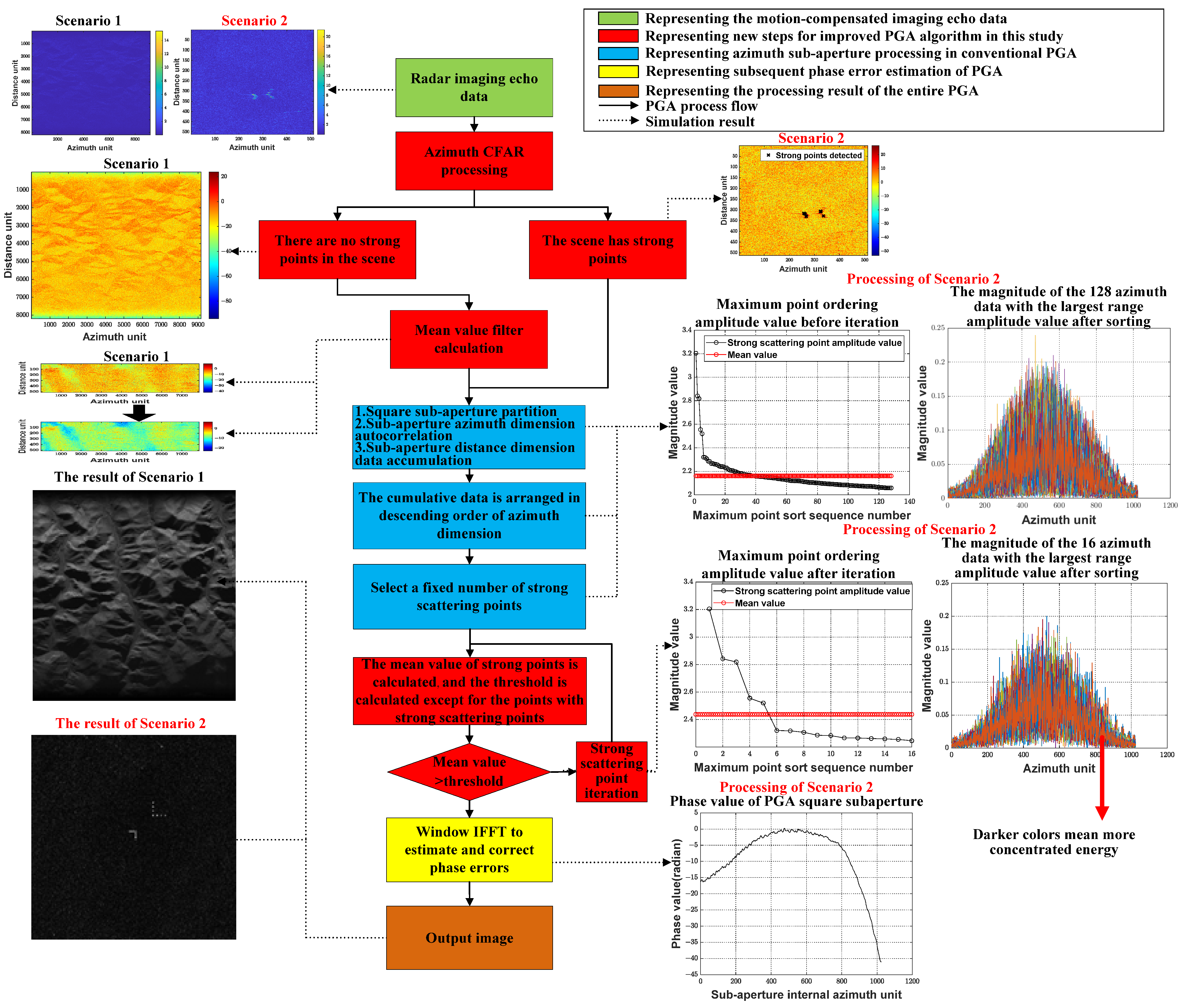
The flowchart of the phase gradient autofocusing method proposed in this study is shown in Figure 3 below.
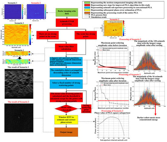
Figure 3.
Improved PGA flowchart. CFAR, constant false alarm rate.
2.2.1. One-Dimensional Azimuth Constant False Alarm Rate (CFAR) Processing
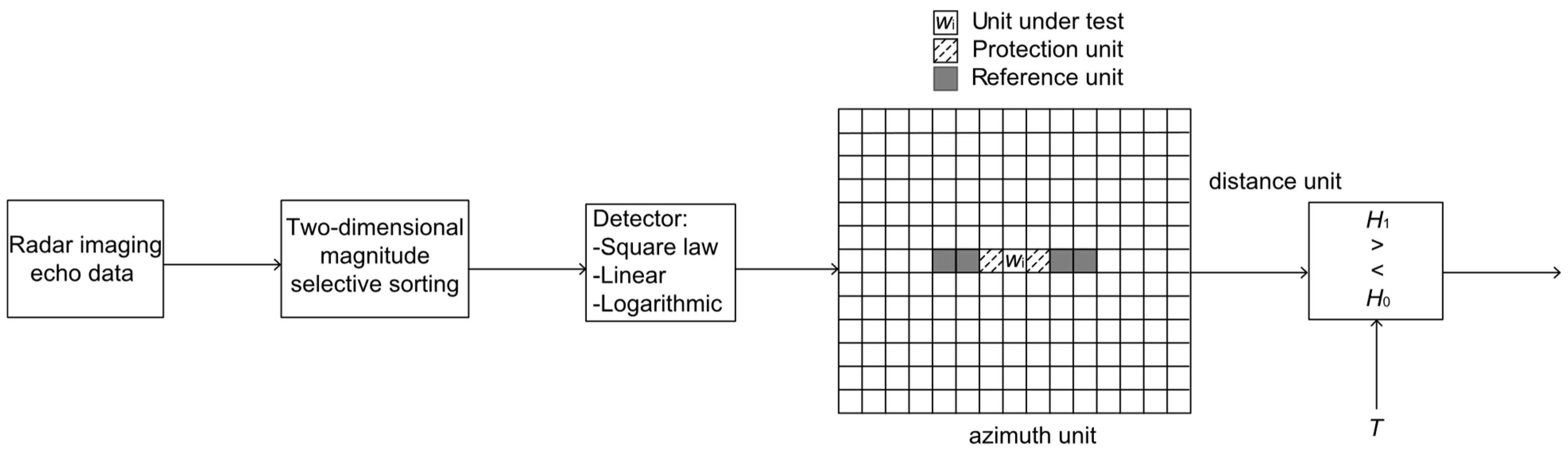
The radar echo data that are subject to SAR motion compensation and other processing are first subjected to azimuth CFAR processing, in order to determine whether there are any strong scattering points in the scene. Then, it is decided whether or not to divide the data into azimuth sub-apertures. As this only involves determining whether there is a strong scattering point in the scene or not, no CFAR target detection is required. Therefore, in this study, we utilize this method to first perform one-dimensional selection of large and clustered values in the imaging data before carrying out PGA to sort the five points with maximal values, following which these five maxima are subjected to a simple one-dimensional azimuth averaging CFAR. If at least one of the five maximum values passes the threshold, it is considered that there are strong scattering points in the scene that require subsequent PGA processing. As this method is used to select the echo data for large cases (with only five points for one-dimensional CFAR detection), it does not lead to a significant increase in computational complexity, and its impact on real-time processing is negligible. The CFAR process used in this study is depicted in Figure 4 below.

Figure 4.
Simple one-dimensional CFAR schematic.
From the above figure, it can be seen that the radar imaging echo data first need to be processed for azimuth dimension selection in each distance cell:
where represents the number of distance units in the radar imaging echo data, is the amplitude matrix after azimuth maxima selection, and is the true azimuth dimensional position information for each maxima stored.
After this one-dimensional maxima determination is carried out, in order to prevent the problem of strong scattering points being surrounded by sub-flaps, resulting in a small range of detected points (due to the large values of the surrounding azimuth units), it is additionally necessary to carry out two-dimensional coalescence processing on the detected points:
where . Through performing two-dimensional coalescence, it is possible to synthesize a point with four distances and azimuths around a certain strong scattering point, which effectively removes the sub-flap effect of the strong scattering point.
After two-dimensional coalescence, the remaining are combined into a one-dimensional array. Then, we select the five largest values that represent the unit to be tested, denoted as , and record the distance orientation information, , of the five units to be tested. Finally, the locations of the five corresponding points are found in the radar imaging echo data prior to one-dimensional azimuth CFAR processing.
The most important step in one-dimensional CFAR processing is to find the detector; that is, the required threshold. In Figure 4, is the cell to be tested, which is in the center. The cells in gray on both sides in the azimuth dimension are data collected earlier (left) and later (right), relative to the radar of the cell to be tested. These are averaged in order to estimate the noise parameters [35]. The cells immediately adjacent to the cells to be detected (marked by crosshairs in the figure) are protection cells, and their corresponding samples are excluded from estimation of the noise parameters. The reason for this treatment is that the same strong scattering point may span multiple azimuth cells, as there may be not only background clutter interference but also the energy reflected from the strong scattering point itself in a protection cell, which tends to be larger than the energy of the clutter interference. This processing serves to raise the threshold of detection.
The azimuth data samples for are averaged as follows:
where represents the sample size for reference cell selection in the azimuth dimension. The number of reference cells in this study was set as 16 [36].
Then, the threshold for carrying out one-dimensional azimuth CFAR can be obtained by multiplying by a factor according to the value obtained from Equation (6) [37]:
where represents the dynamic threshold of the dynamic CFAR, which can be calculated using , where represents the corresponding false alarm probability under the estimated threshold.
Based on the amplitude value corresponding to , the threshold value corresponding to is calculated using Equations (6) and (7). As long as there is a point to be measured in the data that satisfies , it can be assumed that there is a strong scattering point in this image scene, and the subsequent PGA azimuth sub-aperture processing is executed; otherwise, all subsequent PGA processing is directly skipped, and the result is directly output.
2.2.2. Averaging Removing the Bottom Noise
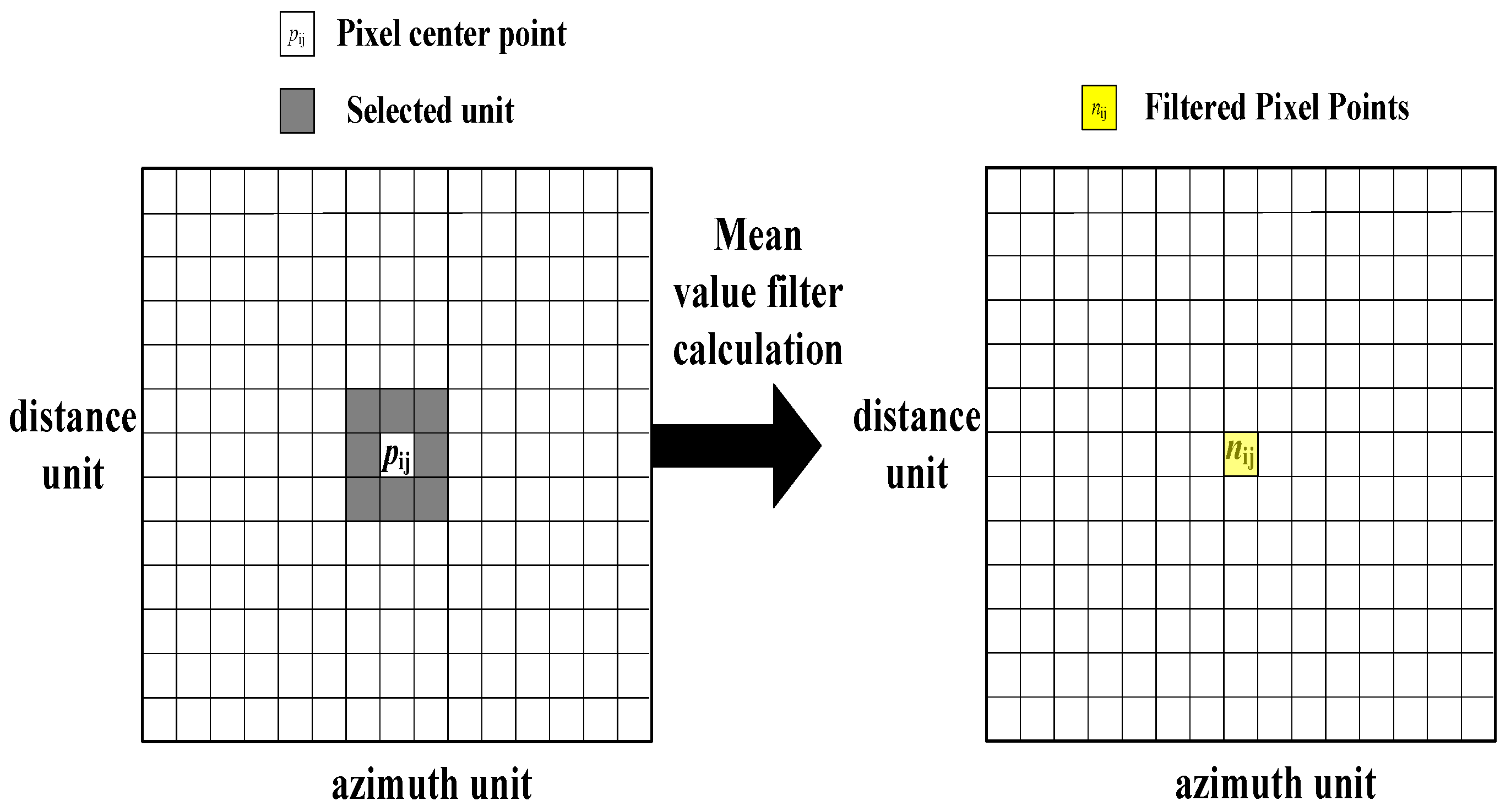
When the processed scene image does not have points that pass the threshold during CFAR detection, this image usually has a low signal-to-noise ratio, which makes the phase error estimated based on the strong scattering points of the image inaccurate. In order to accurately estimate the phase error of the image, the scene image needs to be denoised (this algorithm utilizes a mean filtering process). In the first step, the maximum point location is found in the CFAR detection in the previous processing step, and then, the distance cell where the point is located is intercepted as the center. One-sixteenth of the entire distance cell is intercepted for the bottom noise filtering. In the second step, with each pixel point in the image as the center, the pixel points of 3 × 3 around the center of the image (including the pixel point, if it is a point less than 3 away from the boundary, it is not processed) are subjected to a mean value calculation, and the calculated mean value is given to the pixel point ; is an integer of the interval of , and is an integer of the interval of , wherein denotes the total number of the distance units of the image of the scene, and denotes the total number of the orientation units of the image of the scene. The specific schematic diagram is shown in Figure 5 below.
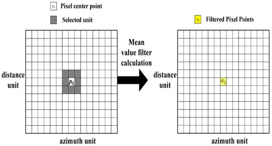
Figure 5.
Schematic diagram of the selected points for denoising by mean filtering.
Through the mean denoising process in Figure 5, the noise floor before PGA processing can be reduced so that the signal-to-noise ratio of the image of the scene without strong scattering points can be improved. Then the denoised part of the image is subjected to subsequent PGA processing, and the resulting phase error value compensates for the phase error of the whole big picture.
2.2.3. Iterative Processing of Strong Scattering Points
When the pending measurement points in the data satisfy , the radar imaging data are divided into azimuth sub-apertures:
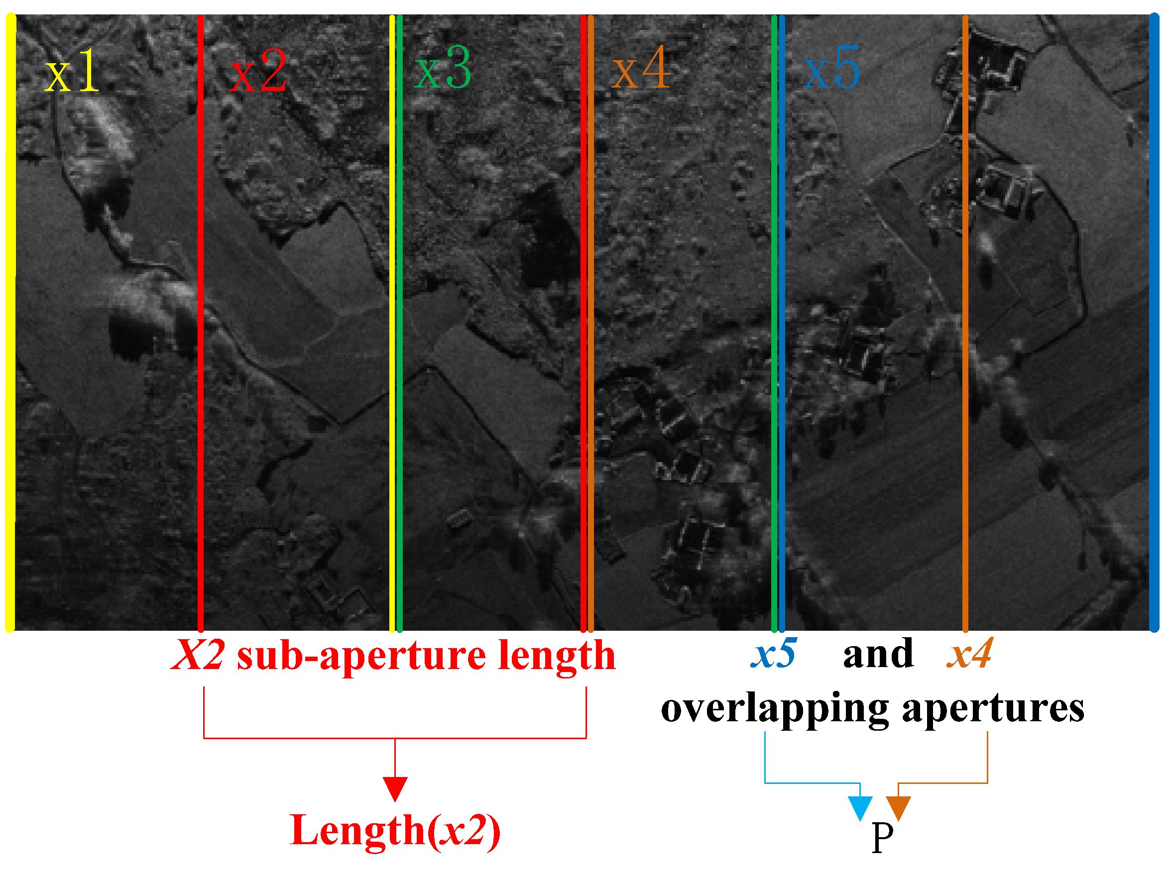
where denotes the radar data processed by the SAR algorithm, denotes the ith set of azimuth sub-aperture data, represents the total number of azimuth sub-apertures, is the length of the azimuth data for each sub-aperture, and is the length of the azimuth sub-aperture overlap. Figure 6 shows the schematic diagram of sub-aperture division.
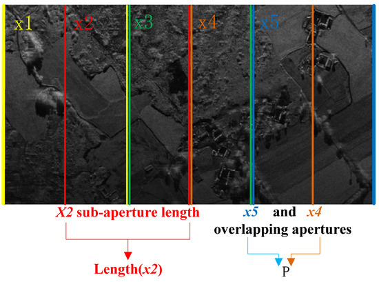
Figure 6.
Schematic diagram of sub-aperture division.
As shown in Figure 6, each delineated azimuth sub-aperture has an overlap of half its length with its neighboring azimuth sub-apertures. The azimuth dimensional autocorrelation algorithm (conjugate multiplication) is then performed on all distance cell data for each azimuth sub-aperture:
where represents the conjugate of the data taken for each distance cell of each sub-aperture, and represents the number of distance cells for each sub-aperture.
The autocorrelation matrix for each distance cell of each azimuth sub-aperture is summed over the data within the sub-aperture:
The azimuth dimensional cumulative data for each azimuth sub-aperture is then sorted in terms of distance:
where yields the descending order of the cumulative data for each azimuth sub-aperture.
Subsequently, in each sub-aperture, it is necessary to carry out judgment of the scene to determine whether the amplitude of the strong scattering points in the scene is sufficiently large. The judgment formula is as follows:
where is the number of strong scattering points selected by default in each azimuth sub-aperture, which can be statistically obtained through simulation of the experimental data; is the mean value of the amplitude of the strong scattering points at a distance in each azimuth sub-aperture; is the mean value of the amplitude of the rest of the points in each azimuth sub-aperture, excluding the strong scattering points at a distance; and is the threshold weight coefficient, which can also be statistically obtained through simulation of the experimental data. If Equation (12) is satisfied, the amplitude of the strong scattering points in the scene is sufficiently large, and the number of selected strong scattering points, , satisfies the requirements for subsequent PGA processing. If is not satisfied, the selection of strong scattering points is continued; the formula for deciding whether to continue selecting strong scattering points is as follows:
The above equation changes the number of strong scattering points for each azimuth sub-aperture from to (if is odd, then is rounded down);conditional judgment is then performed. If the condition is satisfied, the current number of strong scattering points is utilized for subsequent PGA processing. If the condition is not satisfied, the number of strong scattering points is divided by 2, and the mean value is compared until the condition for subsequent PGA processing is satisfied. If the condition is not satisfied when the number of selected strong scattering points is 1, it means that the amplitude of the strong point in the current sub-aperture does not satisfy the threshold requirement, and so, PGA processing is not carried out. This method can be applied to the PGA process for various scenarios, such as towns with many strong scattering points, deserts and beaches with almost no strong points, and scenes with individual strong points (as may occur in desert scenes).
2.2.4. Computational Analysis
The additional steps of the proposed method, compared to conventional PGA, have little effect on the complexity of real-time processing. First, let the number of distance points in each sub-aperture be , the number of azimuth points be , the length of the synthetic aperture be , and the number of selected strong scattering points be . The number of computations associated with conventional PGA can be obtained as follows [32]:
The improved PGA method of this paper is explained from the following three aspects:
Point 1. The one-dimensional azimuth CFAR processing is preceded by one-dimensional elective data enlargement and two-dimensional coalescence. The arithmetic complexity of one-dimensional enlargement is , while that of two-dimensional coalescing is . Subsequently, the number of points used in CFAR detection is only 5, and the size of the reference unit is 16, such that the arithmetic complexity is . Overall, the increased operation volume of this step is
Point 2. If all five points do not satisfy the condition, average the value of the filter to remove noise processing. The number of points for noise filtering in this step totaled , and the amount of operations for cumulative summation and averaging was . Overall, the increased operation volume of CFAR threshold and noise floor filtering is
Point 3. When the PGA selects strong scattering points for iteration, is statistically calculated from the data once and does not need to go through the real-time calculation again. As the strong scattering points are only compared with the non-strong scattering points in the sub-aperture, each iteration has an arithmetic complexity of
where is the number of strong scattering points after the iteration, and represents an integer power of 2. After the number of strong scattering points is changed to , the computational volume of the subsequent PGA processing will be reduced, according to Equation (14). The increase in the number of operations in this step is
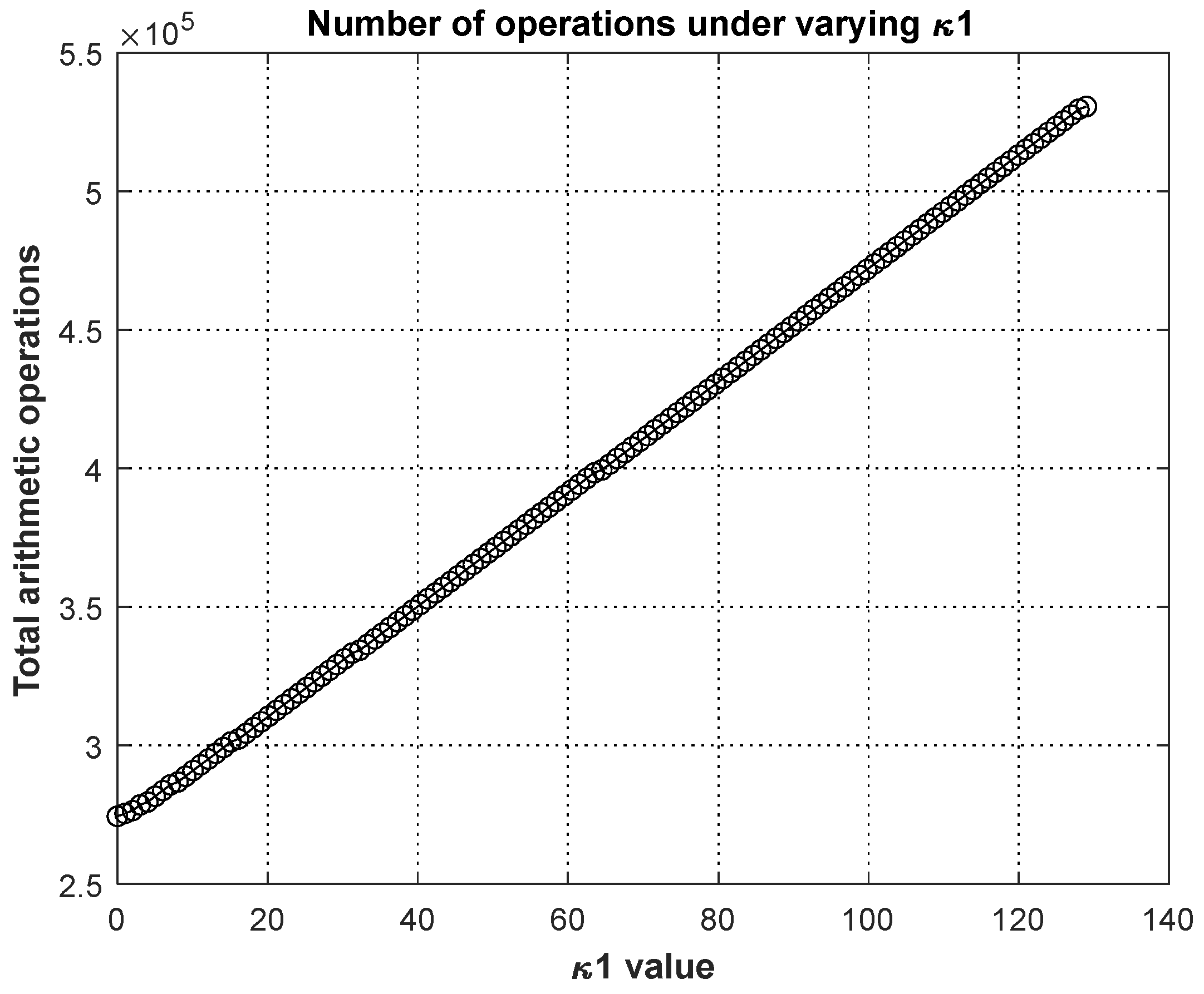
According to the above three considerations, the increases in the amount of arithmetic complexity associated with Equations (15), (16) and (18) are added together. In this study, the initial value of is 128. When in Equation (7), we then set the number of distance points to , the azimuth points to , and the length of the synthetic aperture to . According to Equation (14), the number of arithmetic operations using conventional PGA is 7,078,144, and according to the above parameters—as well as Equations (15), (16) and (18)—the changes in arithmetic complexity are shown in Table 1. Furthermore, the total increase in arithmetic volume as a function of is plotted in Figure 7.

Table 1.
Change in arithmetic complexity under different k1 values.

Figure 7.
Variation in arithmetic operations under different values of k1.
As can be seen from Table 1, when the scene is below the one-dimensional CFAR threshold without subsequent PGA processing, the number of operations is reduced substantially; when the scene is somewhat above the one-dimensional CFAR detection threshold, according to Figure 7, it can be seen that the smaller the value after iteration, the smaller the increase in the number of operations. The increase in the number of operations was the greatest when , with an increase of 7.48% compared to the original algorithm. However, as the system utilized to implement this algorithm uses parallel computing, the overall increase in processing time for this algorithm will not be higher than the theoretical increase (see Section 3 below for specific processing times).
3. Results
The radar used for the collection of the utilized real-world data was an airborne reconnaissance high-resolution radar, the main function of which is radar imaging processing. The radar is a phase reference radar of a certain band. The antenna is installed in the nose direction with a 90° front and side view, with a downward view angle of about 1.5°. For the several scenarios considered in this study, the carrier aircraft flew horizontally at a speed of about 60 m/s. The height of the aircraft’s flight field was about 3000 m.
3.1. Azimuth CFAR Processing
As the improved PGA processing method proposed in this study, as well as Equations (12) and (13), can only be applied in scenes with strong scattering points, judging whether there are strong scattering points in the scene is the first step of the improved PGA algorithm. The experimental results of one-dimensional azimuth CFAR processing on the data of several different scenes before entering the PGA processing are detailed in the following:
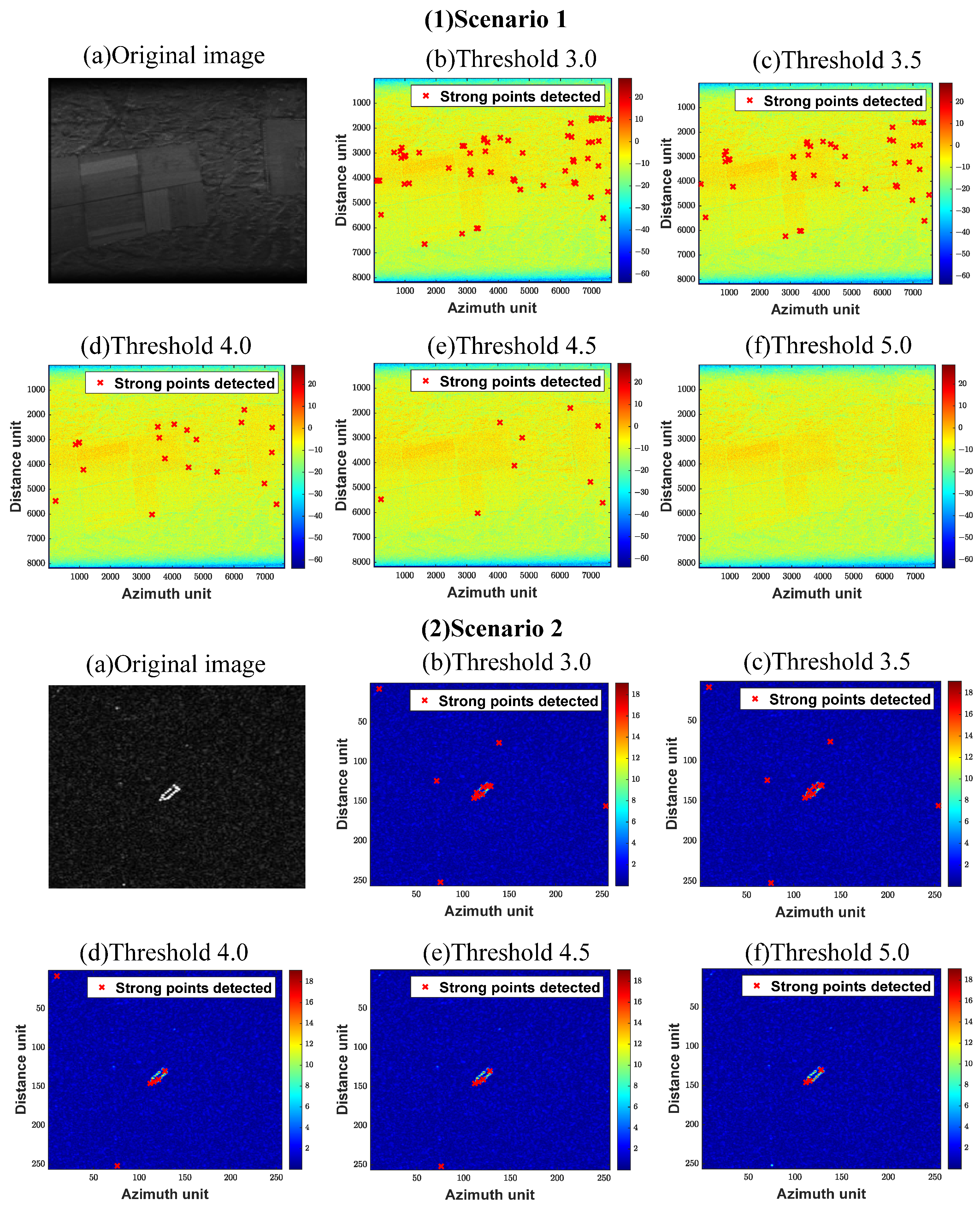
As can be seen from Figure 8, the images were subjected to azimuth CFAR detection prior to PGA processing, and the detected points are shown in Figure 8(1b–1f,2b–2f) and Table 2, where the number of points detected in the image after azimuth CFAR was correlated to (i.e., the dynamic threshold coefficient of CFAR), and fewer points were detected as increased. When , the false alarm rate was only 1.3%, and only strong scattering points that are 13.9794 times higher than the detection threshold value could be detected, indicating that the dynamic threshold is already large. At this time, the points were no longer detected in Scenario 1, while three points were detected in Scenario 2. This indicates that there were strong scattering points in Scenario 2, such that subsequent PGA processing was carried out for Scenario 2, while this processing was skipped for Scenario 1.
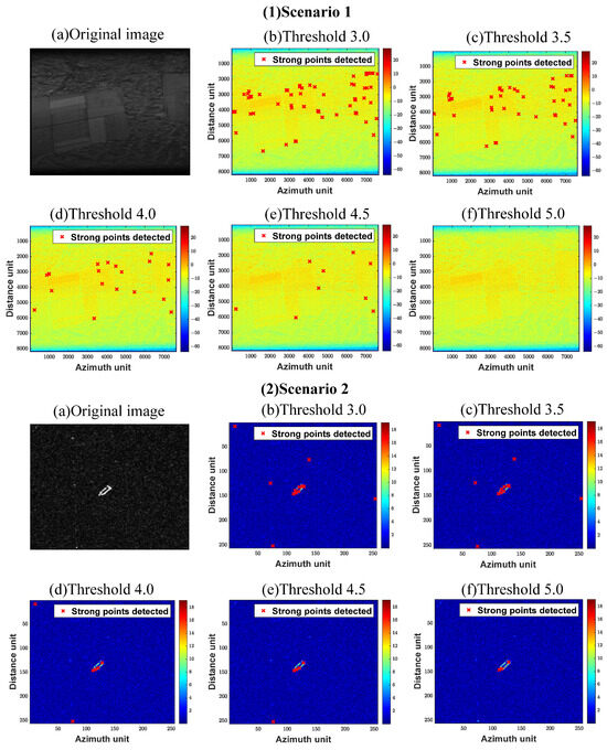
Figure 8.
Image azimuth CFAR detection results before PGA processing.
Table 2.
Number of points detected under varying μ values in CFAR for different scenarios.
3.2. Bottom Noise Removal
This section performs mean filtering of the noise floor for scenes that do not cross the one-dimensional CFAR threshold. The experimental process to determine the image entropy value was as follows:
where is the magnitude of each pixel point in the image, is the number of azimuth points in the whole image, and is the number of distance points in the image. denotes the entropy value of the image, where larger values indicate a more chaotic system.
The PSNR is calculated as follows:
where represents the number of image distance units, represents the number of image distance units, represents the magnitude of each pixel point of the processed image, represents the magnitude of each pixel point of the reference image, represents the mean square error between the processed image and the reference image, and represents the magnitude of the largest point in the amplitude of the processed image. In this study, the reference maps for PSNR are selected from SAR maps of the same scene with special image processing. Its focusing effect is generally recognized.
Table 3 and Figure 9 show the experimental results of the original scene images after PGA processing and after denoising:
Table 3.
Entropy and PSNR calculation of whether or not the image is de-noised.
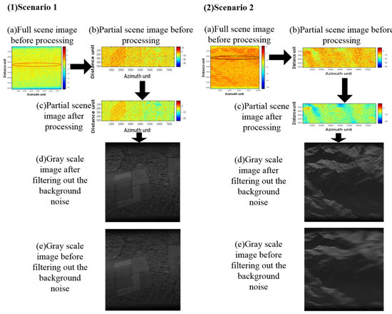
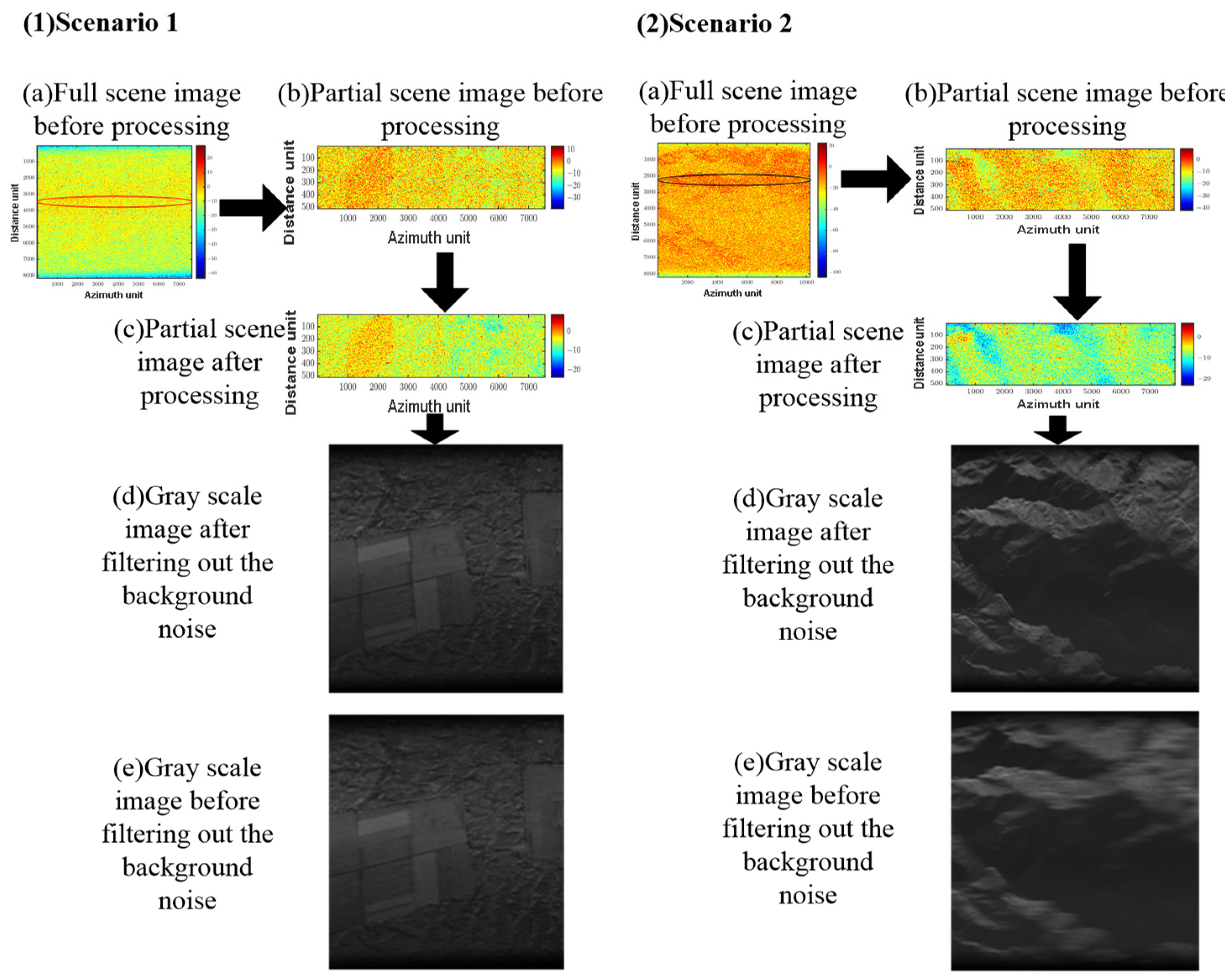
Figure 9.
PGA effect after noise removal.
From Table 3, it can be seen that when there are almost no strong scattering points in the scene, giving the image a mean filter denoising before doing the PGA processing will make the entropy value of the image larger. From Figure 9, it can be seen that the noise floor in the image is significantly suppressed by the denoising process of this method through scene 1 Figure 9(1b,1c) and scene 2 Figure 9(2b,2c). The comparison of Figure 9(1d,1e) and Figure 9(2d,2e) also clearly shows that the quality of the image filtered by the noise floor is better focused.
Therefore, when there is no strong scattering point in the scene and the threshold is not exceeded in CFAR detection, the scene is first rejected by the mean noise floor, and then, PGA processing can make the image focusing effect better than the direct PGA processing focusing effect.
3.3. Determination of k Value
In the PGA calculation process, the distance of the strong scattering points in the scene is selected to estimate the phase error. When selecting the distance of the strong scattering points, the accuracy is not the highest when selecting the strong scattering point with the largest distance. This is because SAR imagery also includes interference due to background clutter, and the good focusing performance of the PGA algorithm is based on the use of a suitable statistical model. If the sample distance for the strong scattering points participating in the estimation process is too small, it can result in inaccurate phase error estimation [38]. This experiment involved PGA processing of a scene utilizing different numbers of strong scattering points. Statistically, the azimuth signal-to-noise ratio of a certain strong scattering point is determined, as shown in Figure 8a.
From Figure 10f–i, it can be seen that, when too few strong scattering points are selected to carry out PGA, the proposed algorithm loses the statistical regularity of the clutter background, and the supporting region around the sample points in the image becomes unstable. From Table 4, it can be seen that, when fewer than 32 points were selected, the image azimuth primary and secondary valve ratios decreased dramatically, thus affecting image focusing. When no fewer than 32 strong scattering points k were selected, it can be seen from Figure 10b–e and Table 4 that the region surrounding the sample points in the image was more stable, and the primary and secondary valve ratio was maintained at ≥21 dB. Based on the above statistics and consideration of the number of arithmetic operations, it was decided that the initial value of for processing all the scenes should be set to 128 points.
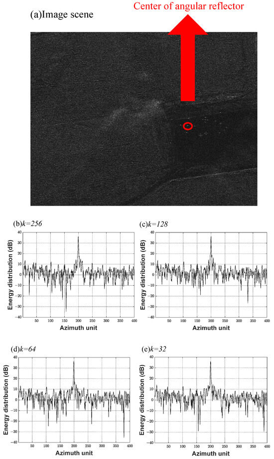
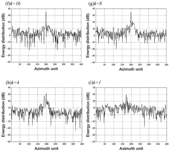
Figure 10.
A scene for which different strong scattering points were utilized for PGA processing (a) and the surrounding energy distribution maps under different values of k (b–i).
Table 4.
Influence of the number of strong scattering points on PGA performance.
3.4. Determination of η Value
For the next experiment, we set and then assessed the focusing effect under different values in multiple scenes and in the same scene.
The focusing effect for two scenes under various values is shown in Figure 11.
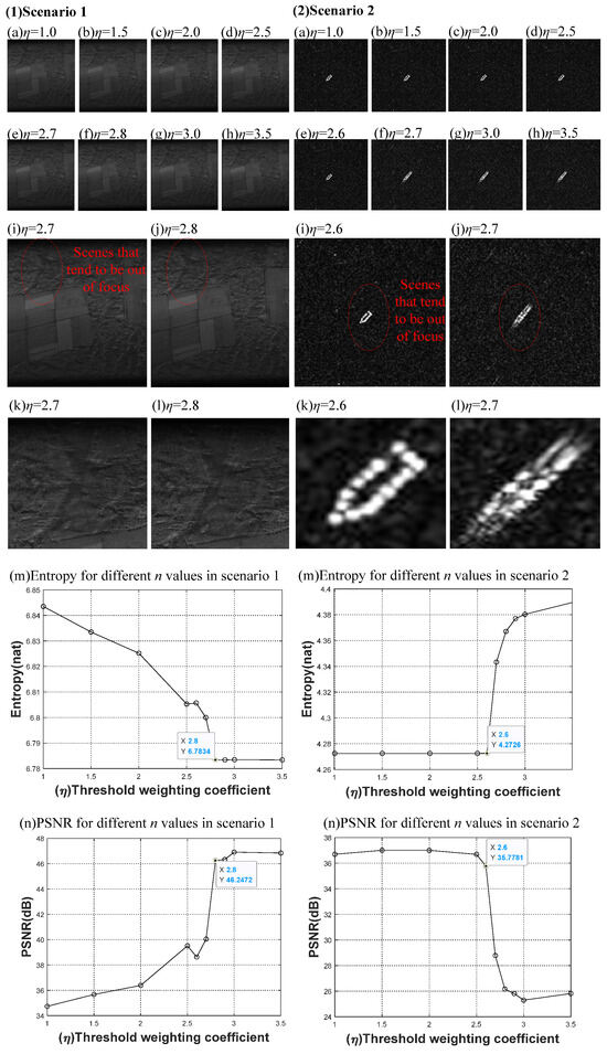
Figure 11.
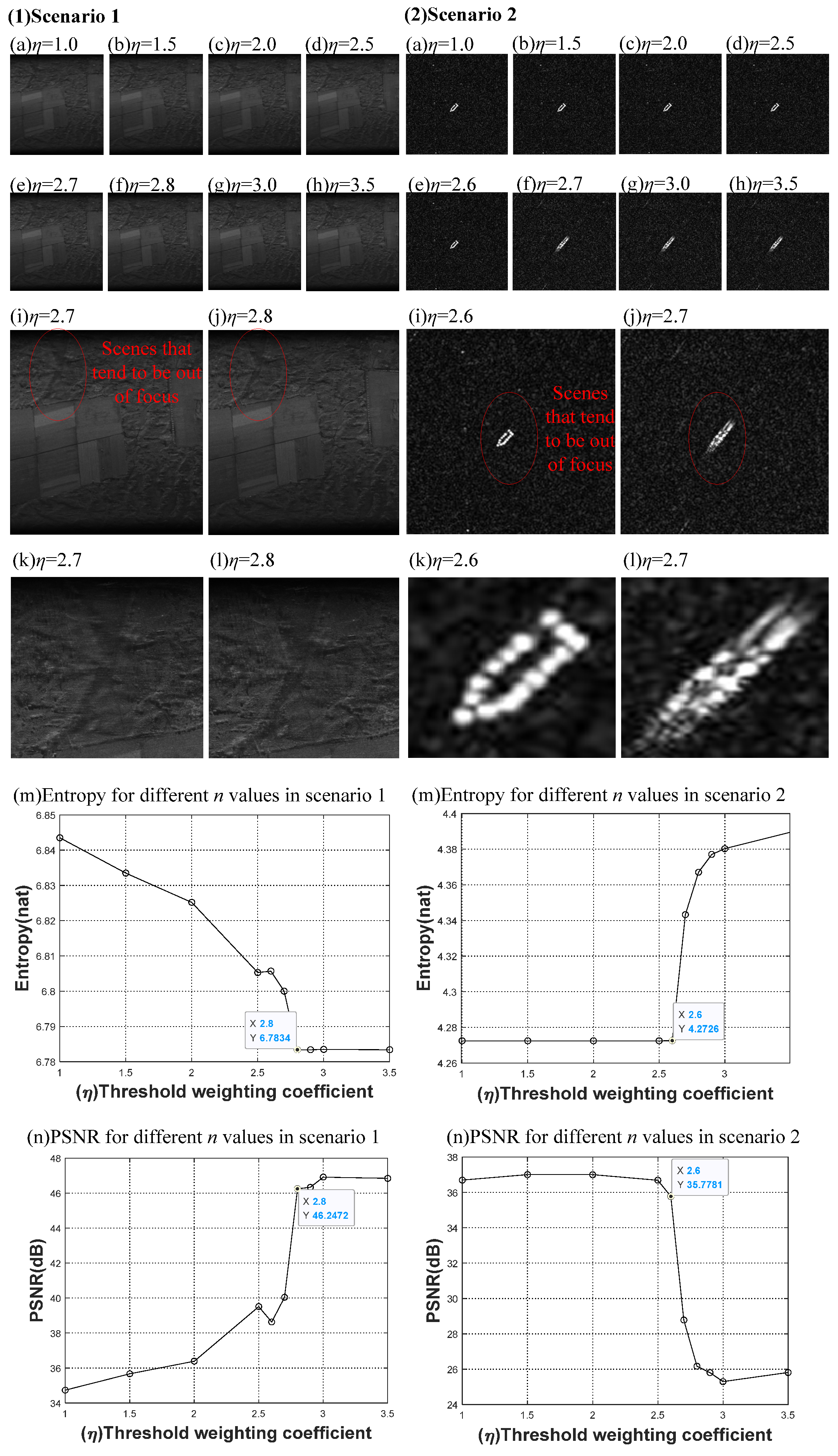
Focusing effect of angular reflector under different η values (a–l), entropy, and PSNR values (m,n) for scenes 1 and 2.
The focusing effect under different values of can be seen in Figure 11(1a–1h). When is small, the focusing effect is poor. The focusing effect was improved when , as shown in Figure 11(1e), but scattering can be observed in Figure 11(1i), with its zoom shown in Figure 11(1k). When , it can be seen from Figure 11(1j)—as well as its zoom shown in Figure 11(1l)—that the position where there is scattering in Figure 11(1k) is better focused. The whole picture can be seen in Figure 11(1j),indicating a good focusing effect. It can also be seen from Table 5 and Figure 11(1m) that the image entropy value was large and fluctuated when . Using the information in Figure 11(1n) and Table 5, it is also known that when , the value of PSNR is relatively small, indicating more image distortion compared to the standard image. Meanwhile, when , the image entropy value and PSNR tend to stabilize. As there are almost no strong points in the scene, the phase error of the strong point estimated by the PGA algorithm was not obtained. It can be seen that, when there is no strong point in the scene (meaning that the image is not defocused), the optimal value of is in the range of . The PGA estimation process is performed when , indicating that the selected strong points are larger than the mean value of the non-strong points, resulting in image defocusing.
Table 5.
Entropy and PSNR calculation for images with different η values.
The focusing effect under different values of can be seen in Figure 11(2a–2e). When was small, the focusing effect was good; however, in Figure 11(2f–2h), angular reflector scattering can be clearly seen. It can also be seen from Table 5, Figure 11(2m,2n),that, when , the entropy value of the image is smaller and tends to stabilize, the PSNR value of the image is larger and also tends to stabilize, and the image is better focused, as can be seen from Figure 11(2i) and its zoom shown in Figure 11(2k). When , the image entropy value was large and fluctuated, the PSNR value of the image was smaller, and the image was defocused, as shown in Figure 11(2j) and its zoomed version in Figure 11(2l). The difference between scenes 1 and 2 is that scene 1 had almost no strong points, such that the image focusing effect will be better without PGA. In contrast, scene 2 presents corner reflectors; therefore, in order to focus on the corner reflectors well, scene 2 should be subjected to PGA processing. It can be seen that, when there are strong scattering points in the scene, in order to prevent the strong scattering points in the image from being scattered, PGA processing must be carried out. At this time, the value is in the range of . The PGA estimation process is not performed when , indicating that the selected strong points are smaller than the mean value of the non-strong points, which results in scattering of the strong points in the image.
In summary, when there is no strong scattering point in the image, in the case of , if PGA processing is carried out, the image will be out of focus. When there is a strong scattering point in the image, in the case of , if PGA processing is carried out, the image will be in focus. It can be inferred that, when the value of is taken near 2.6, regardless of whether there is a strong point in the scene, PGA processing will be carried out—although meets the condition, is too small according to Equations (12) and (13) for strong point amplitude, and regardless of whether the constraints are large enough or not, they will be lowered and the maximum value of will be taken. However, as takes a value of 2.6 when no strong point in the scene is scattered, the selection of strong scattering points must be carried out initially, in order to determine whether any strong points are present (as introduced in Section 3.1).
3.5. Iterative Algorithm Validation
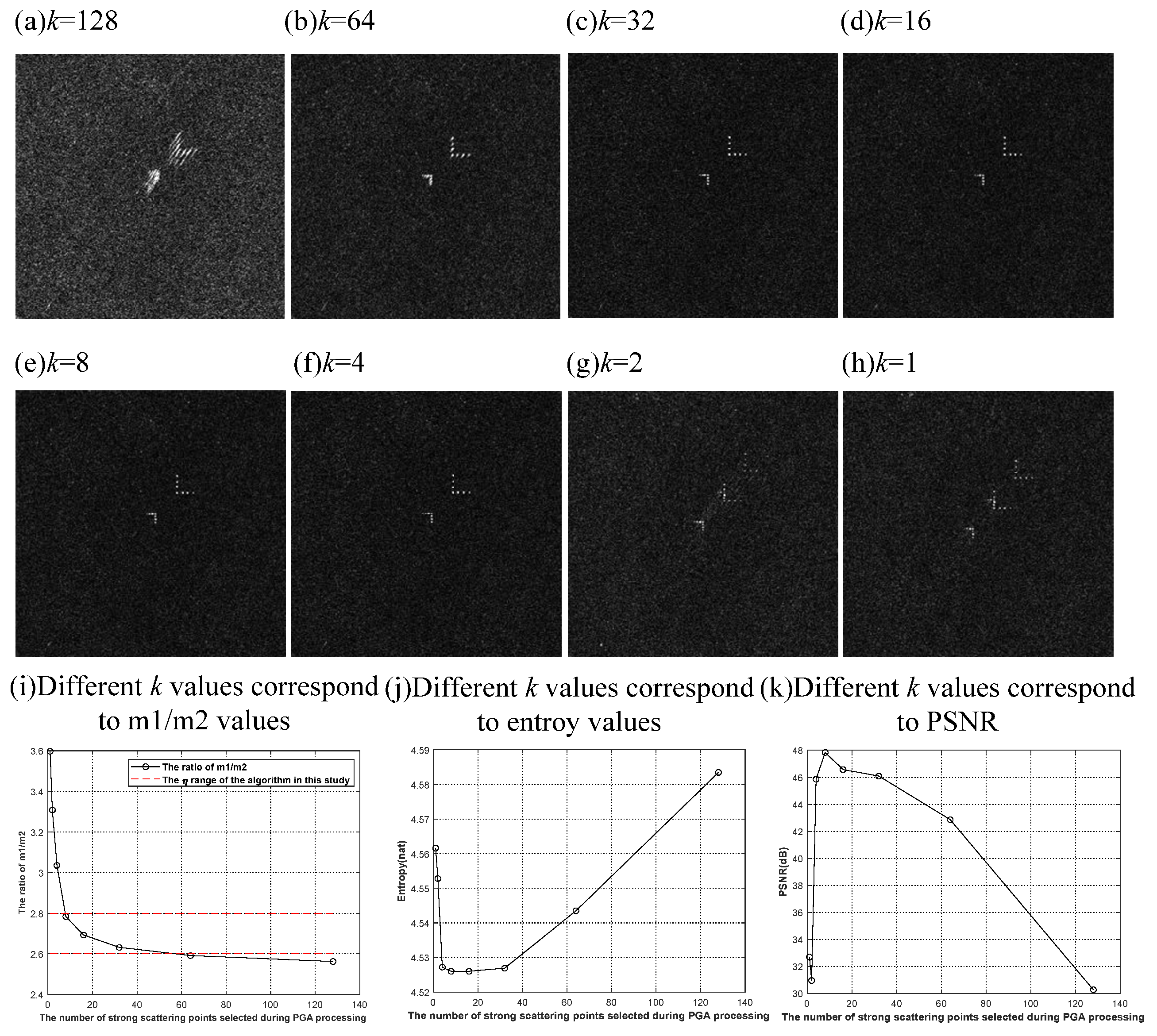
Although it was determined in Section 3.4 that the value of is in the range of 2.6 to 2.8, the above processing was based on the use of for the calculation. For some points in the scene with strong scattering points, the ratio of to calculated under is not in the range of . At this time, the iterative operation of is needed. According to Equation (13), when is smaller, will increase and will decrease, which will make the ratio larger. Through iterating to a certain value that satisfies , the subsequent PGA phase error estimation is performed with the number of strong scattering points at this point. When is reached, if the condition is still not satisfied, the subsequent PGA phase error estimation is not processed. For example, Figure 12a–h show the image focusing effect after selecting different numbers of strong scattering points for PGA phase error estimation in a certain scene. Figure 12i,j and Table 6 show the statistics of , , and , as well as the entropy and PSNR values for different values of in this scene.
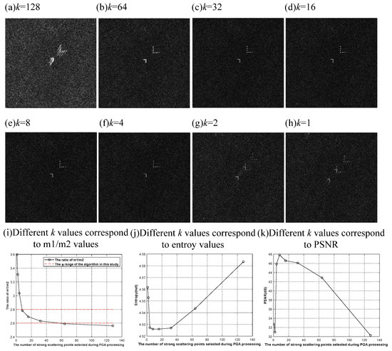
Figure 12.
Plot of PGA treatment effects, with corresponding m1/m2, entropy, and PSNR changes for different values of k in a given scene.
Table 6.
The m1, m2, m1/m2 and entropy values corresponding to different values of k.
As can be seen from Table 6 and Figure 12i, with the calculation of the proposed improved PGA algorithm using , it initially does not satisfy the range of . At this time, the dispersion in the image is shown in Figure 12a, and the entropy value is large in Figure 12j and the PSNR value is small in Figure 12k. Accordingly, Equation (13) is used for iteration, and will be used for the second calculation. It was found that the value of also does not satisfy the range of , and the resulting image is also out of focus. In the next step, using for the calculation, according to Figure 12i and Table 6, is brought into the range of , leading to as mall entropy value and well-focused image. The above results indicate that the PGA processing of this scene at and is not effective, as when using the proposed improved algorithm, from Figure 12i and Table 6, was not in the range of . The iterative computation was thus continued and iterated to for processing. According to Figure 12i and Table 6, the condition was satisfied at , and performing subsequent PGA phase error estimation can achieve good results. Moreover, as shown in Table 6, and were also in the range of and were subjected to subsequent PGA calculations. As can be seen from Figure 12d–k and Table 6, the image entropy and PSNR values were more stable, and the images were well-focused. At the same time, yielded values outside the range of , and according to Figure 12f–h,j,k and Table 6, it can be seen that the entropy values are large and unstable and the PSNR value is small, while the image focusing effect is not only bad, but furthermore, in Figure 12g,h, the images also present heavy shadows.
In summary, the iterative algorithm proposed in this study significantly improves the focusing effect for scenes with strong scattering points and is able to adaptively select the number of strong scattering points for PGA phase error estimation according to the scene.
3.6. Comparative Validation of Algorithms on Real Data
After the above experiments, in order to verify the effectiveness of the improved PGA algorithm proposed in this study, three groups of scenes (the first group with few strong points, the second with almost no strong points, and the third with strong points almost covering the whole scene) were selected for further experiments. In this experiment, we added a two-dimensional advanced algorithm from a well-known university in China and used the data of this algorithm in the experiment as a reference. The obtained experimental results are as follows:
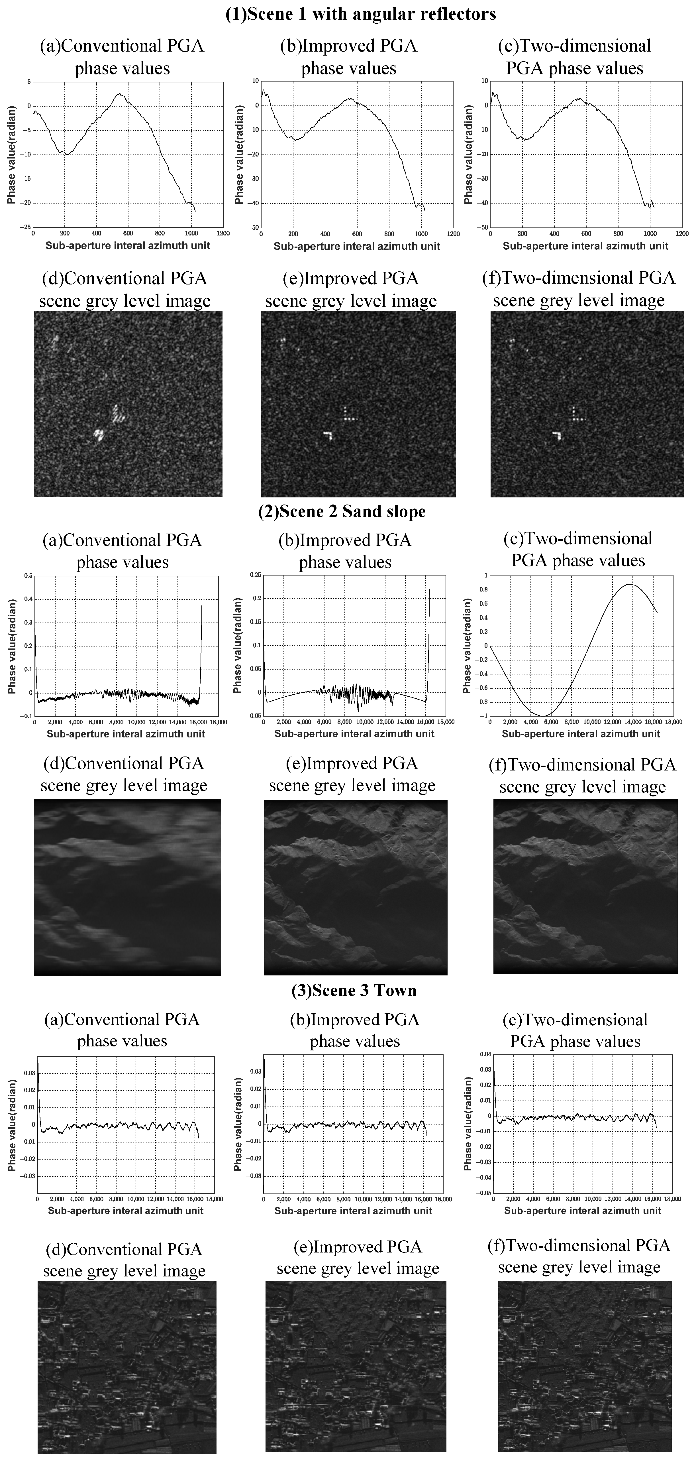
The SAR data from the desert scene with angular reflectors, processed using conventional PGA, two-dimensional PGA, and the proposed improved PGA process, are shown in Figure 13(1a–1f) and Table 7. From Figure 13(1d), it can be seen that applying conventional PGA caused the scene to appear scattered. From the smoother sub-aperture phase error information in Figure 13(1a), it can be concluded that, in the case where there are few strong points in the scene, inaccurate phase estimation will lead to an out-of-focus scene when the phase error is estimated using conventional PGA. The phase error information estimated using the improved method proposed in this study is shown in Figure 13(1b), which follows the same trend as the phase error estimated by the conventional method in Figure 13(1a); however, it is not as smooth when the phase error was estimated using the conventional method, as if each azimuth unit had been stitched together with some gradient variation. The effect of using two-dimensional PGA to process the data of this scene is similar to the improved method in this study in terms of phase estimation in Figure 13(1c) and gray map Figure 13(1f), but the improved PGA is slightly better than the two-dimensional PGA in terms of the entropy and PSNR values in Table 7. Therefore, the processing results shown in Figure 13(1e) are better focused.

Figure 13.
The PGA processing results: (a–c) phase values and (d–f) grayscale images of three scenes (1–3).
Table 7.
Comparison of the entropy and PSNR of the three methods.
Next, the SAR data of sandy slopes were processed using conventional PGA, two-dimensional PGA, and the proposed improved PGA process, as shown in Figure 13(2a–2f). From Figure 13(2d), it can be seen that applying conventional PGA caused the scene to appear scattered. From the large fluctuation in the sub-aperture phase error information in Figure 13(2a), it can be concluded that, in the absence of a strong point in the scene, the phase error estimation using a conventional PGA also resulted in a scattered focus situation due to inaccurate phase estimation. From Figure 13(2f), it can be seen that the image is well focused by utilizing the two-dimensional PGA processing. Similarly, the phase error information estimated after using the improved method in this paper is shown in Figure 13(2b); due to the absence of strong scattering points in the scene, the improved PGA is processed with the removal of bottom noise. Incorrect phase errors are eliminated from the PGA phase error estimation, and the scene focusing effect was significantly improved, as can be seen from Figure 13(2e). However, from Table 7, it can be seen that the two-dimensional PGA is better than the improved PGA in this paper in terms of the entropy and PSNR values. So the focusing effect of this scene is two-dimensional PGA > improved PGA > conventional PGA.
Finally, the SAR data for a town scene were processed using conventional PGA, two-dimensional PGA, and the proposed improved PGA process, as shown in Figure 13(3a–3f) and Table 7. It can be seen that applying the three PGA treatments is comparable in scenes with more strong points, such as the town scene considered here.
3.7. Real-Time Validation
The real-time processing time statistics for the three scenarios detailed in Section 3.6 are provided in Table 8.
Table 8.
Processing time statistics for three different scenarios.
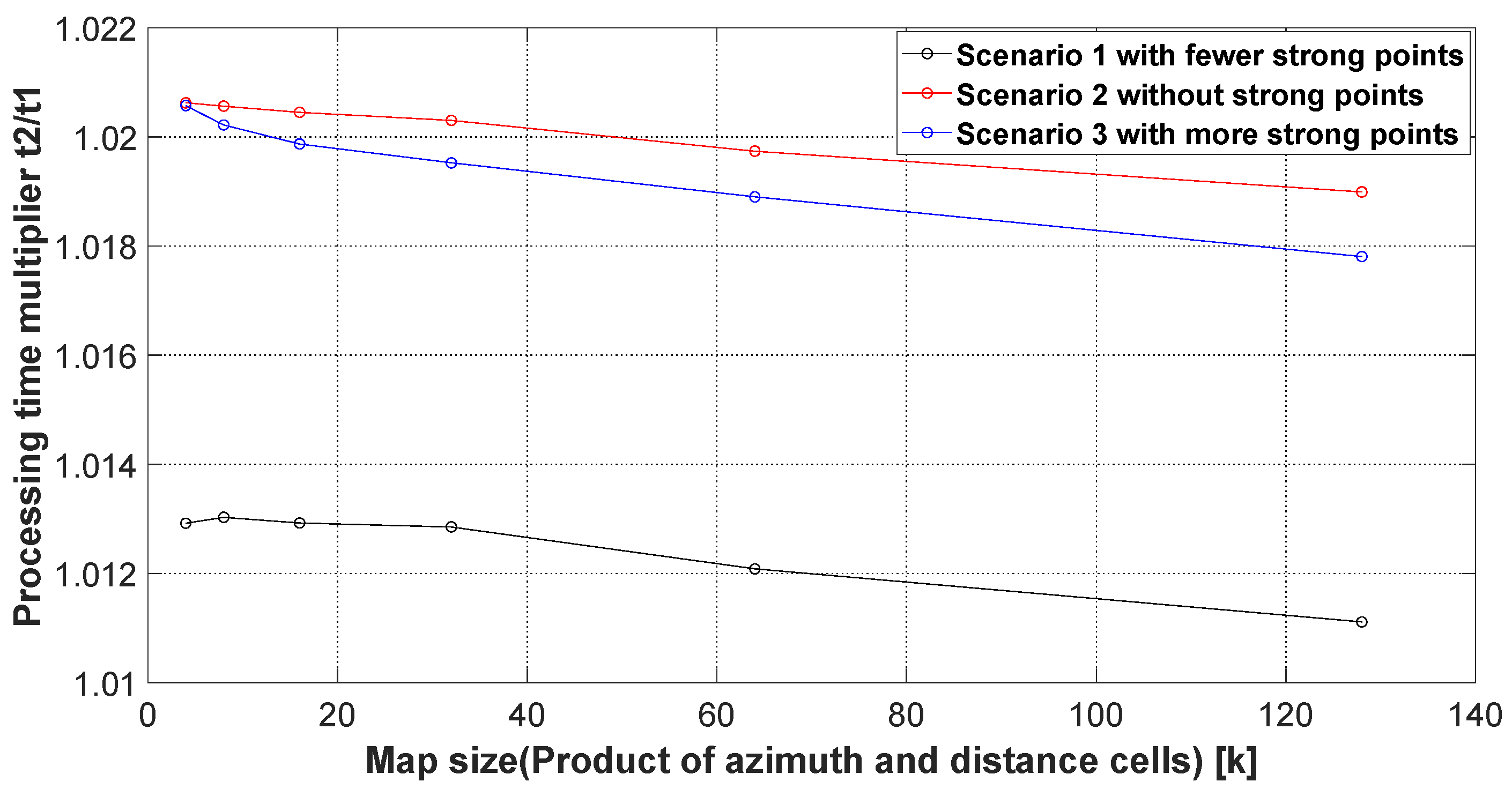
According to Table 8, it can be seen that under the same image size, the processing time of two dimensions is almost two times that of the time of conventional PGA and the improved PGA in this paper, and the processing time of two dimensions is not discussed here. The improved PGA in this study performs mean noise floor filtering after one-dimensional CFAR processing judgment when the scene has no strong points and then performs PGA processing. The processing time increases with the image size from 2.08% for 2 k × 2 k to 1.90% for 8 k × 16 k. When there are strong points in the scene, the maximum time increase using the improved PGA processing in this study does not exceed 2.04%. With the absolute time of 2.4371 s for conventional PGA processing, the increase in time incurred by the improved PGA process will be no greater than 0.05 s. For a 2 k × 2 k image, the shortest time to produce a graph is within the order of 0.5 s, and the increase in the improved PGA over the conventional PGA in this study is in the order of 0.001 s, which affects the time almost negligibly. For 8 k × 16 k images, the shortest time to produce a picture is of the order of 10 s, and the increase in this paper’s improved PGA over the conventional PGA is in the order of 0.01 s, which also affects the time almost negligibly. As can be seen from Figure 14, when the size of the processed image is larger, the improved PGA time in this study and the conventional PGA processing time become closer and closer. This is due to the fact that as the amount of data increases, the multi-core parallel mechanism exerts more and more advantages.
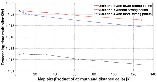
Figure 14.
Comparison curve of processing time between the improved method in this study and the traditional PGA processing time.
4. Conclusions
This study analyzed the shortcomings of the original PGA method from the perspective of determining whether there are strong scattering points in a scene and how many strong scattering points are selected in conventional PGA processing; consequently, an improved PGA processing method was proposed. This method first determines whether there are strong points in the scene; then, it sets the threshold for the scene with strong scattering points by the points in the scene excluding any strong scattering points. By comparing the mean amplitude of the strong scattering points with a threshold, the optimal number of strong scattering points are then used for subsequent PGA processing. For scenes without strong scattering points, the noise floor is removed and then the PGA is performed. It was demonstrated that the improved PGA process significantly improves image focus in scenes that have no or few strong scattering points and does not negatively affect the focus in scenes with sufficient strong scattering points. The processing effect is comparable to the current leading two-dimensional PGA algorithm in China. Meanwhile, the processing time for several scenes was comparable to that of the conventional PGA and faster than that of two-dimensional PGA. Through real flight radar data used to verify the effectiveness of the proposed method, compared with the original method, it could be seen that the focus of the considered images was improved. Overall, using the method proposed in this study can help to improve the clarity and resolution in real-time radar imaging. The biggest novelty of this improved method is that this method will not deteriorate the focusing effect because of the change in scene, and the robustness is stronger than the conventional PGA method. This proposed method has been applied to several airborne projects and achieved good results, which can promote the further development of an airborne imaging radar focusing field. We will continue to refine this direction in our future research.
Author Contributions
Methodology, J.G.; Writing—original draft, C.L.; Writing—review & editing, Y.L.; Visualization, C.H.; Project administration, G.L. All authors have read and agreed to the published version of the manuscript.
Funding
This paper was funded by the National Natural Science Foundation of China under Grant No. 62271363.
Data Availability Statement
The original contributions presented in the study are included in the article, further inquiries can be directed to the corresponding author.
Conflicts of Interest
The authors declare no conflict of interest.
References
- Jiang, R.; Zhu, D.Y.; Zhu, Z.D. A self-focusing algorithm for strip-mode SAR imaging. J. Aeronaut. 2010, 31, 2385–2392. [Google Scholar]
- Cumming, I.; Wong, F. Digital Processing of Synthetic Aperture Radar Data Algorithms and Implementation; Boston Artech House: Norwood, MA, USA, 2005. [Google Scholar]
- Wiley, C.A. Synthetic aperture radars. IEEE Trans. Aerosp. Electron. Syst. 1985, 3, 440–443. [Google Scholar] [CrossRef]
- Song, S.Q.; Dai, Y.P. An effective image reconstruction enhancement method with convolutional reweighting for near-field SAR. IEEE Antennas Wirel. Propag. Lett. 2024, 23, 2486–2490. [Google Scholar] [CrossRef]
- Ge, S.; Feng, D.; Song, S.; Wang, J.; Huang, X. Sparse logistic regression base done-bit SAR imaging. IEEE Trans. Geosci. Remote Sens. 2023, 61, 5217915. [Google Scholar] [CrossRef]
- Xie, Z.; Xu, Z.; Fan, C.; Han, S.; Huang, X. Robust radar wave form optimization under target interpulse fluctuation and practical constraints via sequential lagrange dual approximation. IEEE Trans. Aerosp. Electron. Syst. 2023, 59, 9711–9721. [Google Scholar] [CrossRef]
- Xie, Z.; Wu, L.; Zhu, J.; Lops, M.; Huang, X.; Shankar, B. RIS-aided radar for target detection: Clutter region analysis and joint active-passive design. IEEE Trans. Signal Process. 2024, 72, 1706–1723. [Google Scholar] [CrossRef]
- Ge, S.; Song, S.; Feng, D.; Wang, J.; Chen, L.; Zhu, J.; Huang, X. Efficient near-field millimeter-wave sparse imaging technique utilizing one-bit measurements. IEEE Trans. Microw. Theory Tech. 2024, 72, 6049–6061. [Google Scholar] [CrossRef]
- Song, S.; Dai, Y.; Sun, S.; Jin, T. Efficient image reconstruction methods based on structured sparsity for short-range radar. IEEE Trans. Geosci. Remote Sens. 2024, 62, 5212615. [Google Scholar] [CrossRef]
- Pardini, M.; Papathanassiou, K.; Bianco, V.; Iodice, A. Phase calibration of multibaseline SAR data based on a minimum entropy criterion. In Proceedings of the IEEE International Geoscience and Remote Sensing Symposium, Munich, Germany, 22–27 July 2012; pp. 5198–5201. [Google Scholar]
- Aghababaee, H.; Fornarof, G.; Schirinzi, G. Phase calibration based on phase derivative constrained optimization in multibaseline SAR to mography. IEEE Trans. Geosci. Remote Sens. 2018, 56, 6779–6791. [Google Scholar] [CrossRef]
- Feng, D. Research on Three-Dimensional Imaging Technology of Multi-Baseline SAR. Ph.D. Thesis, National University of Defense Technology, Changsha, China, 2020. [Google Scholar]
- Wahl, D.E.; Eichel, P.H.; Ghiglia, D.C.; Jakowatz, C.V. Phase gradient autofocus—A robust tool for high resolution SAR phase correction. IEEE Trans. Aerosp. Electron. Syst. 1994, 30, 827–835. [Google Scholar] [CrossRef]
- Goodman, W.C.R.; Majewski, R.M. Spotlight Synthetic Aperture Radar Signal Processing Algorithms; Boston Artech House: Norwood, MA, USA, 1995. [Google Scholar]
- Bao, Z.; Xing, M.D.; Wang, T. Radar Imaging Technology; Electronic Industry Press: Beijing, China, 2005. [Google Scholar]
- Sheen, D.R.; VandenBerg, N.L.; Shackman, S.J.; Wiseman, D.L.; Elenbogen, L.P.; Rawson, R.F. P-3 ultra-wideband SAR: Description and examples. IEEE Aerosp. Electron. Syst. Mag. 1996, 11, 25–30. [Google Scholar] [CrossRef]
- Streetly, M. Jane’s Radar and Electronic Warfare System; Janes Information Group: Coulsdon, UK, 1999. [Google Scholar]
- Chan, H.L.; Yeo, T.S. Noniterative quality phase-gradient autofocus (QPGA) algorithm for spotlight SAR imagery. IEEE Trans. Geosci. Remote Sens. 1998, 36, 1531–1539. [Google Scholar] [CrossRef]
- Thompson, D.G.; Bate, J.S.; Arnold, D.V. Extending the phase gradient autofocus algorithm for low-altitude stripmap mode SAR. In Proceedings of the IEEE National Radar Conference, Waltham, MA, USA, 20–22 April 1999; IEEE Press: New York, NY, USA, 1999; pp. 36–40. [Google Scholar]
- Ye, W.; Yeo, T.S.; Bao, Z. Weighted least-squares estimation of phase errors for SAR/ISAR autofocus. IEEE Trans. Geosci. Remote Sens. 1999, 37, 2487–2494. [Google Scholar] [CrossRef]
- Zhai, J.; Wang, J.; Hu, W. Combination of OSELM classifiers with fuzzy integral for large scale classification. J. Intell. Fuzzy Syst. 2015, 28, 2257–2268. [Google Scholar] [CrossRef]
- Sun, X.L. Research on SAR Chromatography and Differential Chromatography Imaging Techniques. Ph.D. Thesis, National University of Defense Technology, Changsha, China, 2012. [Google Scholar]
- Zhang, L.; Wang, G.; Qiao, Z.; Wang, H. Azimuth motion compensation with improved subaperture algorithm for airborne SAR imaging. IEEE J. Sel. Top. Appl. Earth Obs. Remote Sens. 2017, 10, 184–193. [Google Scholar] [CrossRef]
- Zhang, L.; Hu, M.; Wang, G.; Wang, H. Range-dependent map-drift algorithm for focusing UAV SAR imagery. IEEE Geosci. Remote Sens. Lett. 2016, 13, 1158–1162. [Google Scholar] [CrossRef]
- Mao, X.H.; Cao, H.Y.; Zhu, D.Y.; Zhu, Z.D. A priori knowledge-based two-dimensional self-focusing algorithm for SAR. J. Electron. 2013, 41, 1041–1047. [Google Scholar]
- Feng, D.; An, D.; Huang, X.; Li, Y. A phase calibration method based on phase gradient autofocus for airborne holographic SAR imaging. IEEE Geosci. Remote Sens. Lett. 2019, 16, 1864–1868. [Google Scholar] [CrossRef]
- Lu, H.; Zhang, H.; Fan, H.; Liu, D.; Wang, J.; Wan, X.; Zhao, L.; Deng, Y.; Zhao, F.; Wang, R. Forest height retrieval using P-band airborne multi-baseline SAR data: A novel phase compensation method. ISPRS J. Photogramm. Remote Sens. 2021, 175, 99–118. [Google Scholar] [CrossRef]
- Lu, H.; Sun, J.; Wang, J.; Wang, C. A novel phase compensation method for urban 3D reconstruction using SAR to mography. Remote Sens. 2022, 14, 4071. [Google Scholar] [CrossRef]
- Goldschlager, L.M. A universal interconnection pattern for parallel computers. J. ACM 1982, 29, 1073–1086. [Google Scholar] [CrossRef]
- Wang, J.; Leung, K.; Lee, K.; Wang, W. Multiple nonlinear integral for classification. J. Intell. Fuzzy Syst. 2015, 28, 1635–1645. [Google Scholar] [CrossRef]
- Valiant, L.G. A bridging model for parallel computation. Commun. ACM 1990, 33, 103–111. [Google Scholar] [CrossRef]
- Qing, J.-M.; Xu, H.-Y.; Liang, X.-D.; Li, Y.-L. An improved PGA algorithm that can be used for real-time imaging. Radar J. 2015, 4, 600–607. [Google Scholar]
- Wahl, D.E.; Jakowatz, C.V., Jr.; Thompson, P.A. New approach to Strip-Map SAR autofocus. In Proceedings of the IEEE 6th Digital Signal Processing Workshop, Yosemite National Park, CA, USA, 2–5 October 1994; pp. 53–56. [Google Scholar]
- Eichel, P.H.; Ghiglia, D.C.; Jakowatz, C.V. Speckle processing method for synthetic-aperture-radar phase correction. Opt. Lett. 1989, 14, 1–3. [Google Scholar] [CrossRef]
- Tao, X.Y.; Zhang, D.L.; Liu, W.J. Design and realization of a high-speed configurable two-dimensional CFAR detector. J. Hefei Univ. Technol. 2023, 46, 627–631. [Google Scholar]
- Xiao, C.S.; Quang, Z.; Zhu, Y. Improved CAG-CFAR detector based on Grubbs’ law. Radar Sci. Technol. 2020, 18, 682–688. [Google Scholar]
- Mark, R. Fundamentals of Radar Signal Processing, 2nd ed.; Xing, M.D.; Wang, T.; Li, Z.F., Translators; Electronic Industry Press: Beijing, China, 2017; pp. 266–281. [Google Scholar]
- Zhao, M.; Wang, X.L.; Wang, Z.M. Phase gradient self-focusing algorithm for SAR images based on optimal contrast criterion. Remote Sens. Technol. Appl. 2005, 20, 606–610. [Google Scholar]


Disclaimer/Publisher’s Note: The statements, opinions and data contained in all publications are solely those of the individual author(s) and contributor(s) and not of MDPI and/or the editor(s). MDPI and/or the editor(s) disclaim responsibility for any injury to people or property resulting from any ideas, methods, instructions or products referred to in the content. |
© 2025 by the authors. Licensee MDPI, Basel, Switzerland. This article is an open access article distributed under the terms and conditions of the Creative Commons Attribution (CC BY) license (https://creativecommons.org/licenses/by/4.0/).