Abstract
Sea ice motion plays an important role in the seasonal and interannual evolution of the polar sea ice cover. Satellite imagery can be used to track the motion of sea ice via cross-correlation feature tracking algorithms. Such a method has been used for the National Snow and Ice Data Center (NSIDC) sea ice motion product, based largely on passive microwave imagery. This study investigates the use of a new enhanced resolution passive microwave brightness temperature (TB) product to derive ice motion products. The results demonstrate that the new imagery source provides useful daily motion estimates that provide denser spatial coverage and reduced errors. The enhanced TBs yield motions that have a 30% lower Root Mean Square (RMS) difference with motion estimates from buoys. The enhanced resolution TBs will be used in the new version of the NSIDC motion product that is currently in development.
1. Introduction
Sea ice plays an important role in the climate system [1]. It reflects incoming solar radiation and modulates the heat and moisture exchange between the ocean and the atmosphere. It plays a key role in polar ecosystems and impacts human activities. The seasonal and interannual evolution of sea ice is governed by both thermodynamic and dynamic processes. Thermodynamics controls the growth and melt rates via heat transfer between the atmosphere and ocean/ice. Dynamics controls the transport of ice via forcing from wind and ocean currents, ocean topography, Coriolis, and internal ice strength. These dynamic forces can also affect changes in the ice itself. Convergent motion can cause the ice to fracture and pile into ridges that may reach many meters thick, much thicker than level ice. Divergent motion fractures the ice, opening up ice-free regions called leads. In winter, lead formation temporarily increases the heat flux from the open water to the atmosphere as new ice forms and thickens; ice in leads is thinner than surrounding floes. During the melt season, lead formation enhances the absorption of solar energy and enhances the melt of surrounding floes. Thus, observations of sea ice motion are valuable in understanding the state and evolution of the sea ice system. Estimates of ice motion have helped document a regime shift in Arctic Sea ice toward a thinner and more dynamic ice cover [2].
Sea ice motion can be estimated in various ways. A direct method is calculated from the drift of in situ buoys [3] placed on the ice by tracking the change of location over time. Another source for motion estimates comes from remote sensing imagery via feature tracking methods. A common remote sensing source is passive microwave imagery because it provides complete daily coverage of the polar regions in all-sky conditions (except for a small region around the pole), albeit at low spatial resolution. The low spatial resolution limits the motion detail that can be retrieved, and errors can be relatively high at a local scale, e.g., [4]. It is not able to explicitly detect lead formation or ridging. However, it is useful for tracking large-scale motion patterns and long-term variability. The buoy and passive microwave sources have been combined to provide a dataset of gridded sea ice motions [5,6] archived at the NASA National Snow and Ice Data Center (NSIDC) Distributed Active Archive Center (DAAC). Other motion products, such as the EUMETSAT Ocean and Sea Ice Satellite Application Facility (OSISAF) product [7,8], employ similar methods and have similar error characteristics [4].
Here, we present an evaluation of a new source of passive microwave brightness temperatures that are gridded at an enhanced resolution that yields improved motion estimates with lower errors. The enhanced resolution motions are compared with motion estimates from standard resolution imagery via comparisons with buoy-derived motion.
2. Materials and Methods
This study focuses on the use of enhanced resolution passive microwave brightness temperatures (TBs) from the JAXA Advanced Microwave Scanning Radiometer 2 (AMSR2) to estimate sea ice motion. These have recently been published at the NSIDC DAAC as part of the “Calibrated Enhanced-Resolution Passive Microwave Daily EASE-Grid 2.0 Brightness Temperature ESDR, Version 2” (CETB) dataset [9]. The CETB product grids swath TBs at an enhanced resolution via the radiometer form of the Scatterometer Image Reconstruction (rSIR) method [10]. The method uses overlapping sensor footprints to synthesize a higher resolution on a specific grid. The CETB product includes twice-daily TBs on polar EASE2 grids [11] at 3.125 km, 6.25 km, and 12.5 km resolution, depending on the TB frequency. This compares to standard gridded resolutions of 6.25 km, 12.5 km, and 25 km, respectively (Table 1). Here, we use the EASE2 Northern Hemisphere grid (EASE2 North), for which the gridding is conducted based on the local time of day (LOTD), for the morning (centered on 0600 LOTD) and evening (centered on 1800 LOTD). In this study, the 36 GHz and 89 GHz frequencies were used as they provide the most reasonable resolution for ice motion retrieval (discussed further below).

Table 1.
Spatial resolution of AMSR2 frequencies used in this study: the sensor footprint (instantaneous field of view), the enhanced rSIR resolution on the EASE2 North grid, and the standard drop-in-the-bucket resolution.
The gridded resolution of the rSIR fields is a function of the signal-to-noise ratio of the processing and yields a grid spacing that is finer than the effective resolution [12]. The increase in effective resolution over the nominal sensor footprint is 30–50% [13]. For this study, we upsampled (reduced spatial resolution) the 36 GHz 3.125 km rSIR grids to 6.25 km to better match the effective resolution from rSIR. The grids are nested, so the up-sampling was done by a simple average of the TBs of the four (2 × 2) 3.125 km resolution grid cells within each 6.25 km grid cell.
The CETB product also includes a lower standard resolution gridded product. The low-resolution “GRD” fields use a basic drop-in-the-bucket method, where each grid cell averages the sensor footprints whose centers fall within the bounds of the grid cell within the given interval. The GRD fields are all produced at 25 km resolution on the EASE2 grid, regardless of the frequency. However, for AMSR2, the standard resolution is finer than 25 km, and the GRD fields are thus lower than the actual AMSR2 sensor capabilities. Thus, for comparison with the CETB rSIR estimates, we instead use TBs from the NASA “AMSR-E/AMSR2 Unified (AU) L3 Daily [6.25 km and 12.5 km] Brightness Temperatures, Sea Ice Concentration, Motion & Snow Depth Polar Grids, Version 1” [14,15]. These AU products are provided on the NSIDC North and South polar stereographic grids, so the North products were reprojected onto the EASE2 North grid for consistency with the rSIR fields.
Sea ice motion was derived from the passive microwave imagery using a Maximum Cross-Correlation (MCC) method originally developed by [16]. The general approach matches features from one image in a coincident image separated by some time period. A feature in the first image is selected, and then a search box is moved within a search window of the subsequent image to find the correlation peak with the feature in the first image. This correlation peak is assumed to be the new position of the feature in the second image. The displacement is calculated from the change in position of the feature, and the motion velocity is calculated by dividing the displacement distance by the time separation. For passive microwave data, a “feature” is effectively a TB signature of a grid cell that is related to the microwave emissive properties, such as thickness, salinity, snow cover, and surface roughness. It is not a specific feature, such as an individual ice floe. As long as the “feature” stays consistent over the interval, the method is effective for any type of ice, including first-year and multiyear ice. However, when the ice properties are changing rapidly, such as with young and thin ice during freeze-up, the MCC is less effective. The methodology is the same as is used for the NSIDC product [5].
Here, we implemented the MCC method on daily morning rSIR scenes and daily descending AU passes to estimate daily ice motion components (u and v) relative to the EASE2 North polar grid. For the MCC, we use 4X oversampling to obtain sub-grid-cell motion estimates; this is done by shifting the search box in sub-grid increments to obtain a finer location of the correlation peak. After the basic MCC method was run on a pair of images, two post-processing quality control filters were applied. The first is a simple minimum correlation threshold, chosen as 40%. Early in the product development, different thresholds were tested, and 40% was found to have the optimum balance between eliminating erroneous vectors and retaining “good” vectors. The second quality control is a neighborhood filter to remove correlations that are likely erroneous even though they are above the threshold.
For the evaluation of the passive microwave motions, we employed buoys from the International Arctic Buoy Program (IABP) [3]. Noon and midnight buoy positions from the three-hour buoy data were used to calculate 24-h displacements (noon to noon, midnight to midnight) and then averaged to obtain a single one-day displacement on the EASE2 North grid. This was divided by 24 h to obtain daily motion estimates for comparison with the passive microwave data.
As noted above, the motion estimates are limited by the sensor resolution. The footprint of passive microwave radiometers is dependent on frequency, with higher frequencies having smaller footprints and, thus, potentially more precise motion estimates. For this reason, typically, the near-90 GHz channels (89 GHz for AMSR2) have been employed to obtain the finest resolution possible. However, the near-90 GHz channels are more susceptible to atmospheric emission, which can limit retrievals and cause errors in the motion estimates. The 36 GHz channels have less atmospheric influence but coarser spatial resolution (no atmospheric corrections are conducted to the near-90 GHz in the NSIDC product, though such corrections could potentially improve surface retrievals). However, with AMSR2, particularly from the enhanced rSIR TBs, the resolution of the 36 GHz is quite suitable for retrieving motion estimates and is much improved over earlier sensors such as the U.S. Defense Meteorological Satellite Program (DMSP) Special Sensor Microwave Imager (and Sounder) (SSMI and SSMIS), which are used for much of the NSIDC motion product [5]. Previous work, e.g., [8], has found that polarization does not affect the motion retrievals, with both vertical and horizontal polarization channels having equal performance. Thus, here we use the horizontal resolution channels.
The winter period of 1 November 2022 to 30 April 2023 was chosen for the study. Passive microwave radiometers are sensitive to the phase state of water, which allows them to distinguish between sea ice and open water. During late spring and summer, when snowmelt onset begins and liquid water forms on the ice, the signal of ice features is obscured by emission from the surface water. This results in fewer retrievals of motion estimates and with much higher errors. Atmospheric emissions during summer can also inhibit the quantity and quality of motion retrievals. Thus, passive microwave sensors are either not employed during summer [8] or are given a much lower weight [17]. The methodology and data described above are summarized in Table 2.
Table 2.
Summary of the TB sources for this motion study. The grid resolution values correspond to the order of the frequencies in the line above.
3. Results
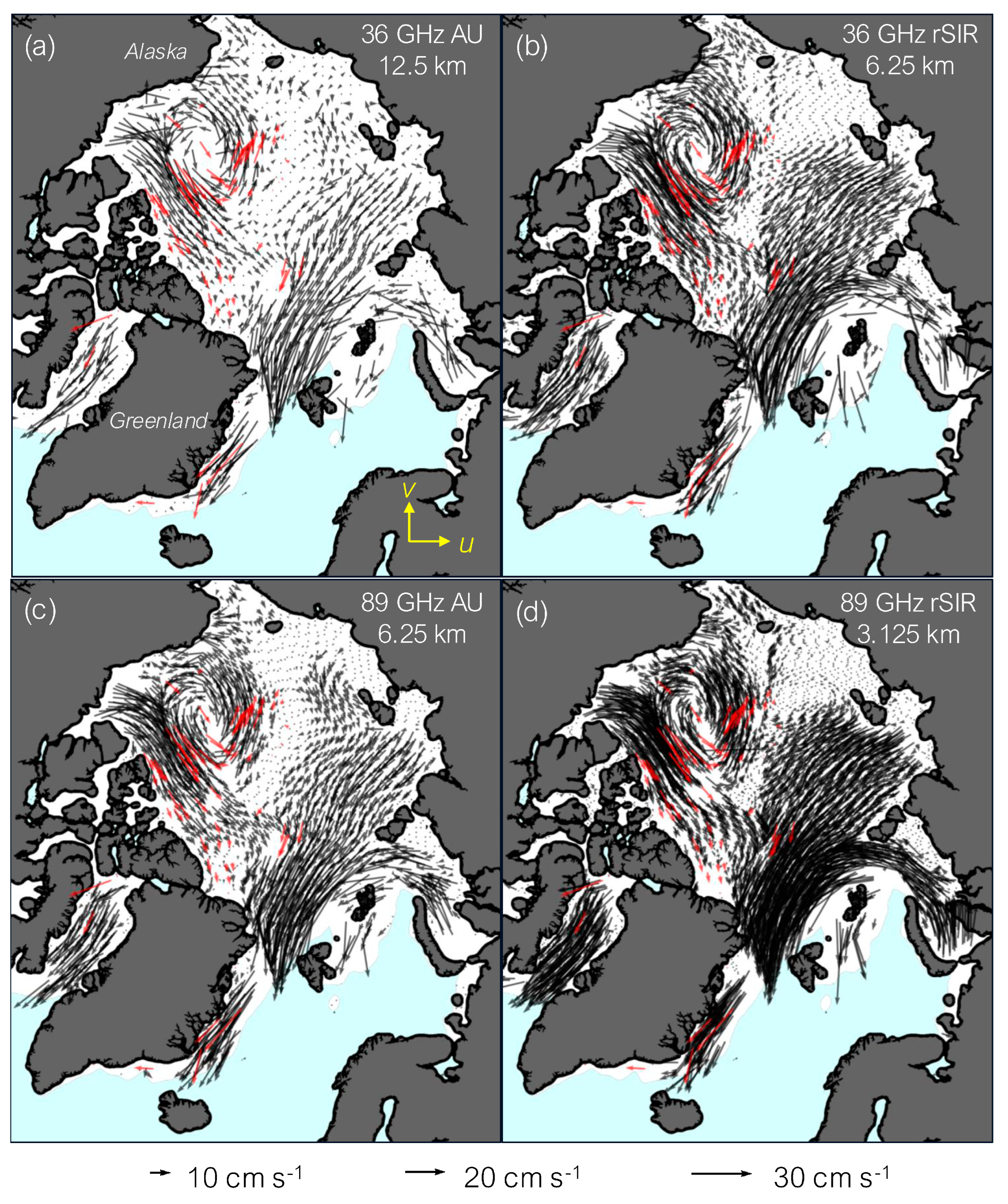
The motion fields are first assessed qualitatively, examining daily maps of the motions. The MCC algorithm yields a motion estimate for every 5th grid cell, so the spacing of motion estimates for TB grid resolutions of 3.125 km, 6.25 km, and 12.5 km is, respectively, 15.625 km, 32.25 km, and 50 km. Thus, higher spatial resolution of the TB fields provides a greater density of estimates. This is seen in daily maps of the motions (Figure 1). For clarity, every 10th motion vector is plotted on each map. All of the fields show similar motion patterns, with a counter-clockwise circulation around a low-pressure center in the Beaufort Sea, a typical transpolar drift from the Siberian coast toward Greenland, and strong outflow through Fram Strait. The AMSR2 vectors also show generally good agreement with buoy motions, with both showing similar motion patterns. However, the agreement is not perfect. Buoy motions are based on the point-to-point motion of a specific sea ice floe, while AMSR2 is tracking a grid-cell-defined region, which may not be consistent with the buoys. Also, the MCC method is limited by the oversampled grid cell resolution, whereas the buoys have no such limitation. Finally, the MCC method can produce an erroneous correlation that is not filtered out and thus yields incorrect vectors.

Figure 1.
Example sea motion fields for 8 March 2023. Black vectors are motions from AMSR2 (a) AU 36 GHz, (b) rSIR 36 GHz, (c) AU 89 GHz, (d) rSIR 89 GHz. Red vectors are buoy motions. The convention for the u and v motion components is illustrated in yellow in (a). The sea ice-covered area is denoted by the white background area. The North Pole is in the center of the image, with the Prime Meridian straight down toward the bottom of the image.
The rSIR maps have twice as many vectors at half the spacing as the standard resolution AU maps, so they show a more detailed and more defined motion pattern. For example, the center of the low in the Beaufort Sea is clearer and more structured in the rSIR fields. Of note, the 36 GHz rSIR TBs have the same gridded resolution as the 89 GHz AU TBs, so the two motion fields have the same density of estimates. However, the 36 GHz frequency is less affected by the atmosphere and can provide higher-quality motions. Thus, rSIR is able to provide the higher quality that 36 GHz delivers at a spatial resolution and density of coverage as the standard 89 GHz.
Next, the AMSR2 motions were compared to buoy motions to quantitatively evaluate and compare the rSIR and AU motions from 36 GHz and 89 GHz TBs. For the comparison, for each buoy, the closest AMSR2 estimate was selected with a maximum radius of 50 km. If there was no AMSR2 estimate within 50 km of a buoy, no comparison was made. Comparisons were made for each day for all available buoys for u and v components of motion relative to the EASE2 Grid (u motion in the x-direction, positive to the right; v motion in the y-direction, positive to the top). For each day of the study period, the AMSR2 minus buoy average difference and the RMS of the difference (RMSd) are calculated.
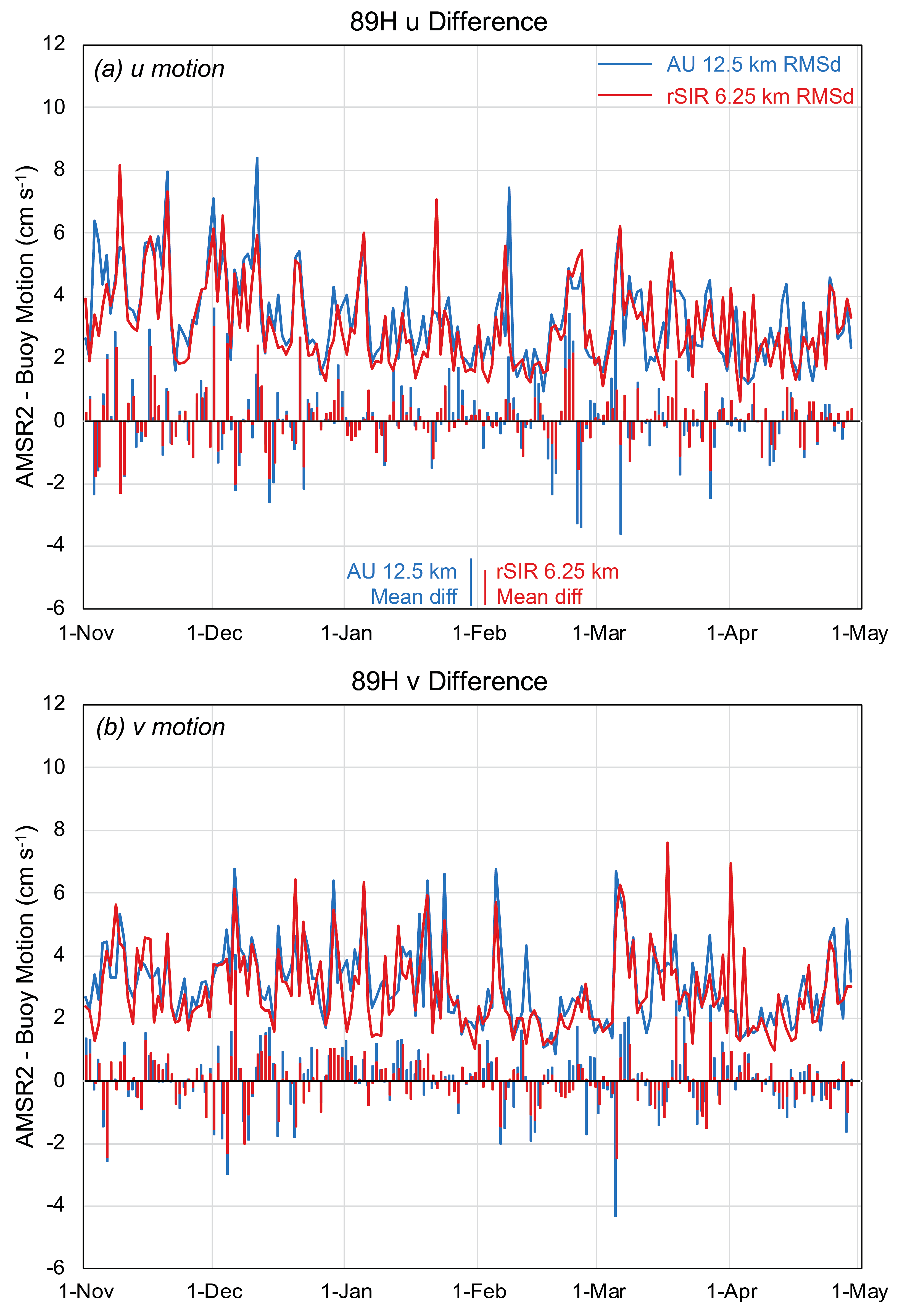
There is a lot of day-to-day variability in both the mean difference and RMSd, reflecting variability in the motions themselves (Figure 2 and Figure 3). For the 36 GHz motions, the rSIR u and v motion components have lower magnitude average differences and lower RMSd for nearly every day (Figure 2); this illustrates that the rSIR TBs provide improved motions over motions from the standard resolution AU TBs. For the 89 GHz motions, there appears to be somewhat less difference, particularly for the RMSd values. On several days, the AU and rSIR motion RMSd lines nearly overlap, and there are more days with the rSIR RMSd higher than AU than the 36 GHz comparison.
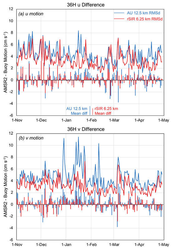
Figure 2.
Time series of daily mean and RMS differences between buoy and AMSR2 36 GHz (a) u component and (b) v component motions. The line plot indicates daily RMSd values, and the thin bars represent the mean difference (bias).
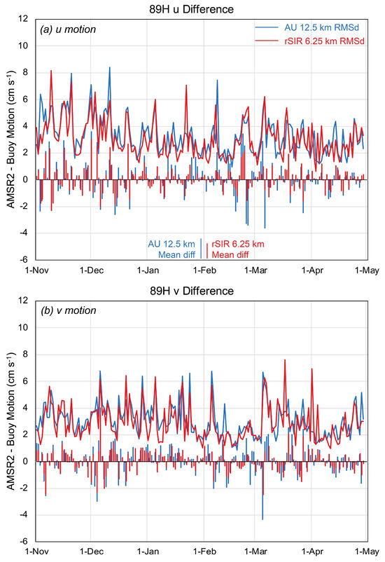
Figure 3.
Time series of daily mean and RMS differences between buoy and AMSR2 89 GHz (a) u component and (b) v component motions. The line plot indicates daily RMSd values, and the thin bars represent the mean difference (bias).
The daily motion characteristics are confirmed in the overall statistics (Table 3) of the comparisons with buoys. The average differences (biases) between AMSR2 and buoys are small for both AU and rSIR, less than 0.5 cm s−1. The rSIR biases are generally smaller or nearly the same. The largest effect of the enhanced resolution is on the RMSd. For 36 GHz, the rSIR motion RMSd is 1 to 1.5 cm s−1 lower than AU, an improvement of ~25% to ~33%.
Table 3.
Average difference and RMSd between AMSR2 and buoys for AU and rSIR TB sources for u and v components.
As seen in the daily comparisons, there is much less improvement for the 89 GHz motions. This is not surprising because the sensor footprint of AMSR2 89 GHz (3 km × 5 km) is nearly the same as the rSIR gridded product (3.125 km). So, rSIR is not doing much resolution enhancement for 89 GHz TB. However, the rSIR method provides much more precise gridding than the simple drop-in-the-bucket method used for the AU product. So, the 89 GHz rSIR motions are still improved over the AU motions, but the improvement (5–10%) is smaller than for 36 GHz.
It is also worth noting that the rSIR motions from 36 GHz have similar differences as the AU motions from 89 GHz. So, as seen qualitatively in Figure 1, rSIR can provide 36 GHz motions of the same character as the AU 89 GHz motions with less of an atmospheric effect.
4. Discussion
Here, we have presented a comparison of sea ice motions derived from AMSR2 TBs for both standard gridded resolution (AU product) and enhanced resolution (rSIR). These are daily motion estimates. As noted earlier, the quality of the motions is limited by the spatial resolution and precision of the temporal sampling. Even with the rSIR enhancement, the resolution is coarse compared to many sea ice dynamical processes, such as ridging and lead formation. So, while these motions are improved, they are most suitable for larger-scale sea ice circulation. There is also uncertainty in the time separation because the TBs are gridded from multiple swaths that cross at different times of the day. The CETB use of a local time of day gridding provides some improvement, but TBs in grid cells between two consecutive days will normally be separated by a time other than 24 h. These limitations are substantial contributors to the RMSd values relative to buoys.
Because of these limitations, some products [8] employ a two- or three-day separation between TB images for the feature correlation. This smooths out “noise” in the daily products and can reduce RMSd values. However, a longer time separation between images can reduce feature correlation as the sea ice surface changes (e.g., snow characteristics, deformation, melt) and reduce the amount and quality of the motion retrievals. Thus, the approach here is to use daily imagery and then average the daily motions over a desired time interval. Spatially interpolating motions, such as using a weighted optimal interpolation scheme, can also reduce RMSd, albeit at the loss of fine-scale details. This is employed in the NSIDC product to reduce errors and to combine the multiple sources into an integrated field.
Summer retrieval of ice motions is challenging because of surface melt. Thus, motion fields in the NSIDC and OSISAF products [5,6,7] augment summer motions with wind-forced motion estimates and either substantially lower the weight of passive microwave fields or do not use them at all during the melt season. However, previous research has shown that the 18.7 GHz channel, which is less affected by surface melt, has the potential to retrieve useful motions during summer [18]. The primary limitation of 18.7 GHz is the large sensor footprint that limits the spatial resolution of the motion retrievals. This presents the intriguing possibility of using the enhanced-resolution CETB 18.7 GHz frequency to obtain improved summer motions at a useful spatial resolution. Future work will investigate the feasibility of using the AMSR2 18.7 GHz channels (and the SSMIS 19.3 GHz channels) and optimally integrating them with buoys and wind-forced motions for summer motion estimates.
5. Conclusions
The current NSIDC sea ice motion product, Version 4 [5,6], is currently being regularly updated with motions derived from standard resolution SSMIS TBs, buoys, and wind-derived parameterization. It also employs AMSR-E and visible imagery as a source for earlier periods. A new version is in development, which will add AMSR2 as a source. This will substantially improve the quality of the estimates. The new source for all passive microwave TBs will be the CETB product, so even SSMIS and earlier passive microwave sources will have improved resolution.
After the development of the new version of the product, we will conduct further validation studies and compare them with other similar motion datasets, such as the OSI-SAF product [7,8]. Advantages of the new product. Intercomparison—plan to do intercomparison with OSI-SAF and other products. It is important to understand the differences between products, but there is value in having multiple independent products. Like global temperature, sea ice extent, and other climate products, an “ensemble” of estimates provides greater context of the variability of a geophysical parameter and can reveal biases and potential errors in processing. The new version of the NSIDC sea ice motion product will be a valuable addition to the current suite of sea ice motion estimates.
Author Contributions
Conceptualization, W.N.M. and J.S.S.; methodology, W.N.M. and J.S.S.; software, J.S.S.; validation, W.N.M. and J.S.S.; formal analysis, J.S.S. and W.N.M.; investigation, W.N.M. and J.S.S.; resources, W.N.M.; data curation, J.S.S.; writing—original draft preparation, W.N.M.; writing—review and editing, J.S.S.; visualization, J.S.S. and W.N.M.; supervision, W.N.M.; project administration, W.N.M.; funding acquisition, W.N.M. All authors have read and agreed to the published version of the manuscript.
Funding
This research was funded by the NASA Cryospheric Sciences Program, grant number 80NSSC21K0763.
Data Availability Statement
The source CETB data are available from the NSIDC DAAC at the referenced DOI. Derived motions are currently available from the authors on request; they will be published with the new version of the NSIDC motion product.
Acknowledgments
Thanks to M.J. Brodzik and the NSIDC DAAC Data Production Team for providing early access to the CETB AMSR2 data during the initial part of this study. We also gratefully acknowledge the essential contributions of Chuck Fowler, University of Colorado, who passed away on 13 February 2023. He originated the MCC method for the product and developed the initial version of the NSIDC sea motion dataset; the more recent advancements of the motion product stand on the shoulders of his work.
Conflicts of Interest
The authors declare no conflicts of interest.
References
- Meier, W.N.; Hovelsrud, G.; van Oort, B.; Key, J.; Kovacs, K.; Michel, C.; Granskog, M.; Gerland, S.; Perovich, P.; Makshtas, A.P.; et al. Arctic sea ice in transformation: A review of recent observed changes and impacts on biology and human activity. Rev. Geophys. 2014, 52, 185–217. [Google Scholar] [CrossRef]
- Sumata, H.; de Steur, L.; Divine, D.V.; Granskog, M.A.; Gerland, S. Regime shift in Arctic Ocean sea ice thickness. Nature 2023, 615, 443–449. [Google Scholar] [CrossRef] [PubMed]
- IABP. International Arctic Buoy Program [Data Set]. Available online: https://iabp.apl.uw.edu (accessed on 5 May 2023).
- Sumata, H.; Lavergne, T.; Girard-Ardhuin, F.; Kimura, N.; Tschudi, M.A.; Kauker, F.; Karcher, M.; Gerdes, R. An intercomparison of Arctic ice drift products to deduce uncertainty estimates. J. Geophys. Res. Oceans 2014, 119, 4887–4921. [Google Scholar] [CrossRef]
- Tschudi, M.; Meier, W.N.; Stewart, J.S.; Fowler, C.; Maslanik, J. Polar Pathfinder Daily 25 km EASE-Grid Sea Ice Motion Vectors; Version 4; [Data Set] NSIDC-0116; NASA National Snow and Ice Data Center Distributed Active Archive Center: Boulder, CO, USA, 2019. [CrossRef]
- Tschudi, M.; Meier, W.N.; Stewart, J.S. Quicklook Arctic Weekly EASE-Grid Sea Ice Motion Vectors; Version 1; [Data Set] NSIDC-0748; NASA National Snow and Ice Data Center Distributed Active Archive Center: Boulder, CO, USA, 2019. [CrossRef]
- OSI SAF. Global Low Resolution Sea Ice Drift Data Record 1991–2020 (v1); [Data Set] OSI-455; EUMETSAT Ocean and Sea Ice Satellite Application Facility: Darmstadt, Germany, 2022. [Google Scholar] [CrossRef]
- Lavergne, T.; Down, E. A climate data record of year-round global sea-ice drift from the EUMETSAT Ocean and Sea Ice Satellite Application Facility (OSI SAF). Earth Syst. Sci. Data 2023, 15, 5807–5834. [Google Scholar] [CrossRef]
- Brodzik, M.J.; Long, D.G.; Hardman, M.A. Calibrated Enhanced-Resolution Passive Microwave Daily EASE-Grid 2.0 Brightness Temperature ESDR; Version 2; [Data Set] NSIDC-0630; NASA National Snow and Ice Data Center Distributed Active Archive Center: Boulder, CO, USA, 2024. [CrossRef]
- Long, D.G.; Brodzik, M.J. Optimum Image Formation for Spaceborne Microwave Radiometer Products. IEEE Trans. Geosci. Rem. Sens. 2016, 54, 2763–2779. [Google Scholar] [CrossRef] [PubMed]
- Brodzik, M.J.; Billingsley, B.; Haran, T.; Raup, B.; Savoie, M.H. EASE-Grid 2.0: Incremental but Significant Improvements for Earth-Gridded Data Sets. ISPRS Int. J. Geo-Inf. 2012, 1, 32–45. [Google Scholar] [CrossRef]
- Meier, W.N.; Stewart, J.S. Assessing the potential of enhanced resolution gridded passive microwave brightness temperatures for retrieval of sea ice parameters. Remote Sens. 2020, 12, 2552. [Google Scholar] [CrossRef]
- Long, D.G.; Brodzik, M.J.; Hardman, M. Evaluating the effective resolution of enhanced resolution SMAP brightness temperature image products. Front. Remote Sens. 2023, 4, 1073765. [Google Scholar] [CrossRef]
- Meier, W.N.; Comiso, J.C.; Markus, T. AMSR-E/AMSR2 Unified L3 Daily 6.25 km Polar Gridded 89 GHz Brightness Temperatures; Version 1; [Data Set] AU_SI6; NASA National Snow and Ice Data Center Distributed Active Archive Center: Boulder, CO, USA, 2018. [CrossRef]
- Meier, W.N.; Markus, T.; Comiso, J.C. AMSR-E/AMSR2 Unified L3 Daily 12.5 km Brightness Temperatures, Sea Ice Concentration, Motion & Snow Depth Polar Grids; Version 1; [Data Set] AU_SI12; NASA National Snow and Ice Data Center Distributed Active Archive Center: Boulder, CO, USA, 2018. [CrossRef]
- Ninnis, R.M.; Emery, W.J.; Collins, M.J. Automated extraction of pack ice motion from advanced very high resolution radiometer imagery. J. Geophys. Res. 1986, 91, 10725–10734. [Google Scholar] [CrossRef]
- Tschudi, M.A.; Meier, W.N.; Stewart, J.S. An enhancement to sea ice motion and age products at the National Snow and Ice Data Center (NSIDC). Cryosphere 2020, 14, 1519–1536. [Google Scholar] [CrossRef]
- Kwok, R. Summer sea ice motion from the 18 GHz channel of AMSR-E and the exchange of sea ice between the Pacific and Atlantic sectors. Geophys. Res. Lett. 2008, 35, L03504. [Google Scholar] [CrossRef]

Disclaimer/Publisher’s Note: The statements, opinions and data contained in all publications are solely those of the individual author(s) and contributor(s) and not of MDPI and/or the editor(s). MDPI and/or the editor(s) disclaim responsibility for any injury to people or property resulting from any ideas, methods, instructions or products referred to in the content. |
© 2025 by the authors. Licensee MDPI, Basel, Switzerland. This article is an open access article distributed under the terms and conditions of the Creative Commons Attribution (CC BY) license (https://creativecommons.org/licenses/by/4.0/).