Hybrid Offset Position Encoding for Large-Scale Point Cloud Semantic Segmentation

Abstract

In recent years, large-scale point cloud semantic segmentation has been widely applied in various fields, such as remote sensing and autonomous driving. Most existing point cloud networks use local aggregation to abstract unordered point clouds layer by layer. Among these, position embedding serves as a crucial step. However, current methods of position embedding have limitations in modeling spatial relationships, especially in deeper encoders where richer spatial positional relationships are needed. To address these issues, this paper summarizes the advantages and disadvantages of mainstream position embedding methods and proposes a novel Hybrid Offset Position Encoding (HOPE) module. This module comprises two branches that compute relative positional encoding (RPE) and offset positional encoding (OPE). RPE combines explicit encoding to enhance position features through attention, learning position bias implicitly, while OPE calculates absolute position offset encoding by considering differences with grouping embeddings. These two encodings are adaptively mixed in the final output. The experiment conducted on multiple datasets demonstrates that our module helps the deep encoders of the network capture more robust features, thereby improving model performance on various baseline models. For instance, PointNet++ and PointMetaBase enhanced with HOPE achieved mIoU gains of 2.1% and 1.3% on the large-scale indoor dataset S3DIS area-5, 2.5% and 1.1% on S3DIS 6-fold, and 1.5% and 0.6% on ScanNet, respectively. RandLA-Net with HOPE achieved a 1.4% improvement on the large-scale outdoor dataset Toronto3D, all with minimal additional computational cost. PointNet++ and PointMetaBase had approximately only a 0.1 M parameter increase. This module can serve as an alternative for position embedding, and is suitable for point-based networks requiring local aggregation.

1. Introduction

In recent years, point cloud analysis has gained increasing attention, particularly for tasks such as semantic segmentation or classification, which are used to interpret and utilize the information in 3D point clouds and apply it in various fields, such as urban mapping in remote sensing, 3D architectural modeling, autonomous driving in robotics, and smart home assistants. Point cloud semantic segmentation tasks include small-scale object-level and large-scale scene-level tasks. Given that precise perception of 3D scenes is a critical task in remote sensing, this paper primarily focuses on issues related to large-scale point clouds.

As the point cloud is unordered and permutation-invariant, traditional convolutional neural networks (CNNs) cannot be directly applied to them. The PointNet [1] pioneered the use of symmetric functions to aggregate point clouds, establishing itself as a pioneer of end-to-end point-based networks. However, this method disregards local structures and performs poorly on downstream tasks requiring fine-grained features, making it unsuitable for large-scale scene-level tasks. Consequently, PointNet++ [2] introduced a local structure by searching for neighbors and aggregating them, allowing the network to perform dense prediction tasks. Due to the effectiveness of local aggregation, many methods have built upon this approach, including [3,4,5,6,7,8,9,10,11]. These methods use neighborhood search algorithms, such as ball query or KNN, to establish local neighborhoods and apply different aggregation functions.

The focus of this study is an essential aspect of the local aggregation process: the spatial relationships between points. Without spatial relationships, two central points that share the same neighbors may receive the same signal, causing confusion between their features. Although points are unstructured data, they exhibit spatial autocorrelation properties in Euclidean space.

To model spatial relationships, methods such as [2,6,8,12] utilize the coordinates inherent to point clouds, concatenating the relative coordinates of neighboring points with their features before feeding them into an MLP to establish spatial relationships. However, as the depth of the encoder increases, the number of feature channels for point features grows while the channel count for relative coordinates remains at three, creating an imbalance between coordinate and feature channels that weakens spatial positional relationships in high-dimensional feature space. Ref. [7] addresses this by mapping relative coordinates to the same channel dimension as neighboring features, enhancing the model’s positional information in deeper layers, but this method adds unnecessary computational overhead.

Methods like [4,5,13,14,15,16] use relative coordinates to generate weight kernels that are multiplied with neighboring features and then summed, dynamically adjusting point features to build spatial relationships. However, this spatial-variant kernel prediction incurs significant computation and memory costs, making it unsuitable for deep, sparse point clouds.

In recent works such as [9,10,17], positional information is introduced through positional encoding. Here, neighboring point relative coordinates are mapped to the same dimension as the neighboring features and fused by element-wise addition, which resolves the dimensional imbalance and reduces computation. However, in these methods, relative positional information is mapped to higher dimensions using only a simple MLP, which can lead to the loss of fine-grained positional details in deeper network layers, limiting the model’s ability to fully leverage positional awareness. Ref. [18] also points out that using a single MLP to embed positional bias directly results in similar biases between neighboring points, potentially confusing their relative positions. In addition, the deep encoder places more emphasis on the global information of the point cloud, while the relative position encoding focuses solely on the spatial relationships of points within the local receptive field.

A straightforward solution is to explicitly encode coordinates as position structure descriptors and integrate them with point features, ensuring that points at different coordinates in Euclidean space have distinct position encodings in high-dimensional feature space. For example, ref. [19,20] use trigonometric functions to encode 3D points into high dimensions, while [21,22] utilize relative coordinates as weights to pool neighboring features without requiring learnable parameters. However, this approach may introduce strong biases, making it unsuitable for most networks, as [9] also notes that non-data-driven positional embeddings could disrupt learned point neighborhood features.

Thus, the challenge lies in establishing rich, high-dimensional spatial relationships in deeper layers without compromising the learned features or increasing computational costs excessively. To address this, we propose Hybrid Offset Position Encoding (HOPE). The following outlines the main steps.

Firstly, we implicitly learn positional biases and employ explicit structural encoding in the form of attention to guide the learning process, reducing the impact of outlier points. Additionally, to consider the spatial relationships between points within the global receptive field, we calculate the offset position encoding in the global receptive field, referencing the computation of offset features. This establishes a richer global spatial relationship, which is adaptively added to the relative position encoding, allowing the information to complement each other (as shown in Figure 1). To balance channel dimensions and reduce computational overhead, the generated positional encoding merges positional information with neighboring features in the form of a bias and is applied only in the deeper layers of the encoder. This approach leverages high-dimensional feature space, where spatial relationships are often overlooked, and deeper layers, where point resolution decreases and point count significantly reduces, avoiding a dramatic increase in parameter count and FLOPs.

In summary, our contributions are as follows:

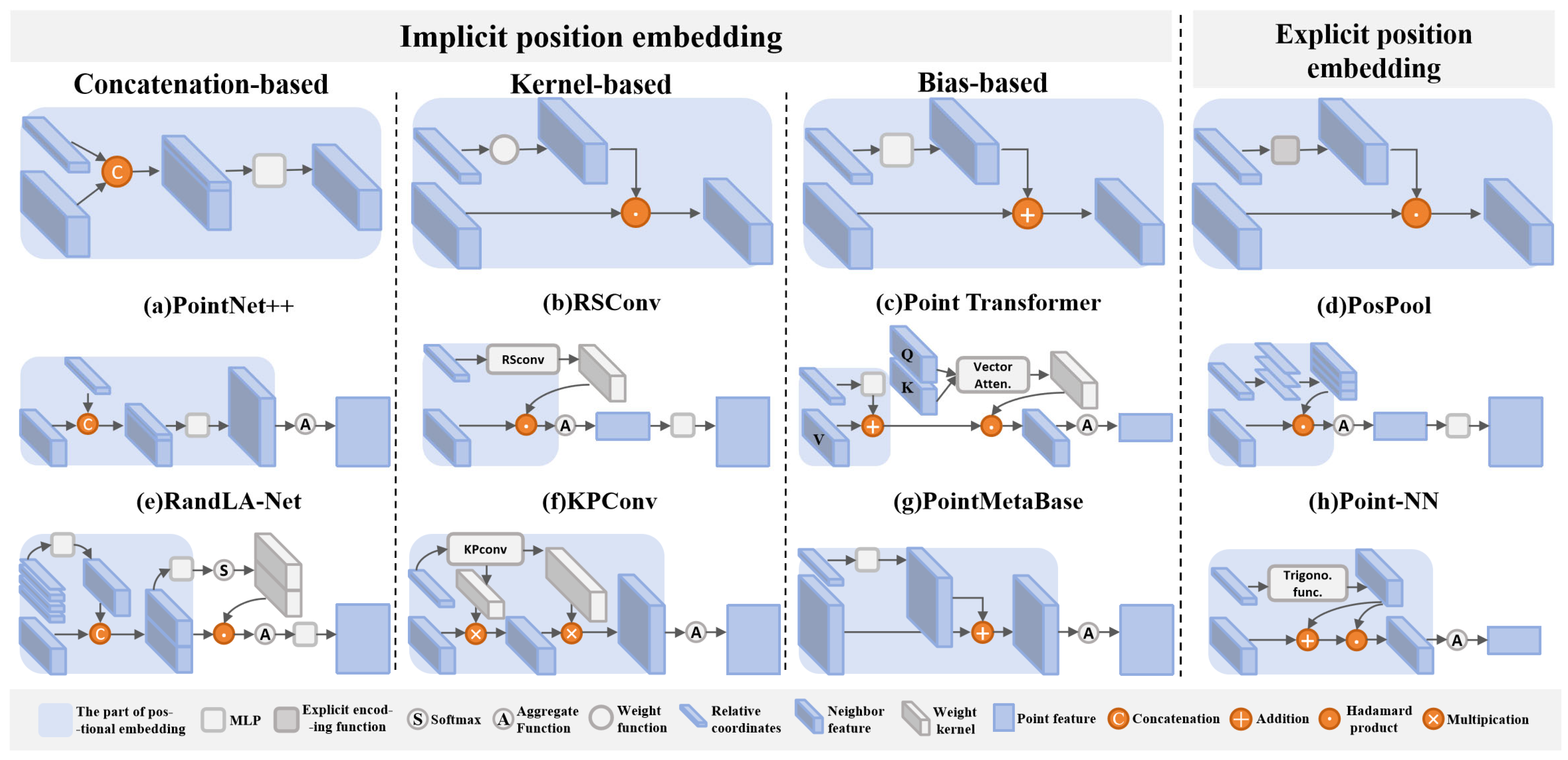
• We review current mainstream positional embedding methods, compare these methods intuitively, and summarize their advantages and disadvantages.
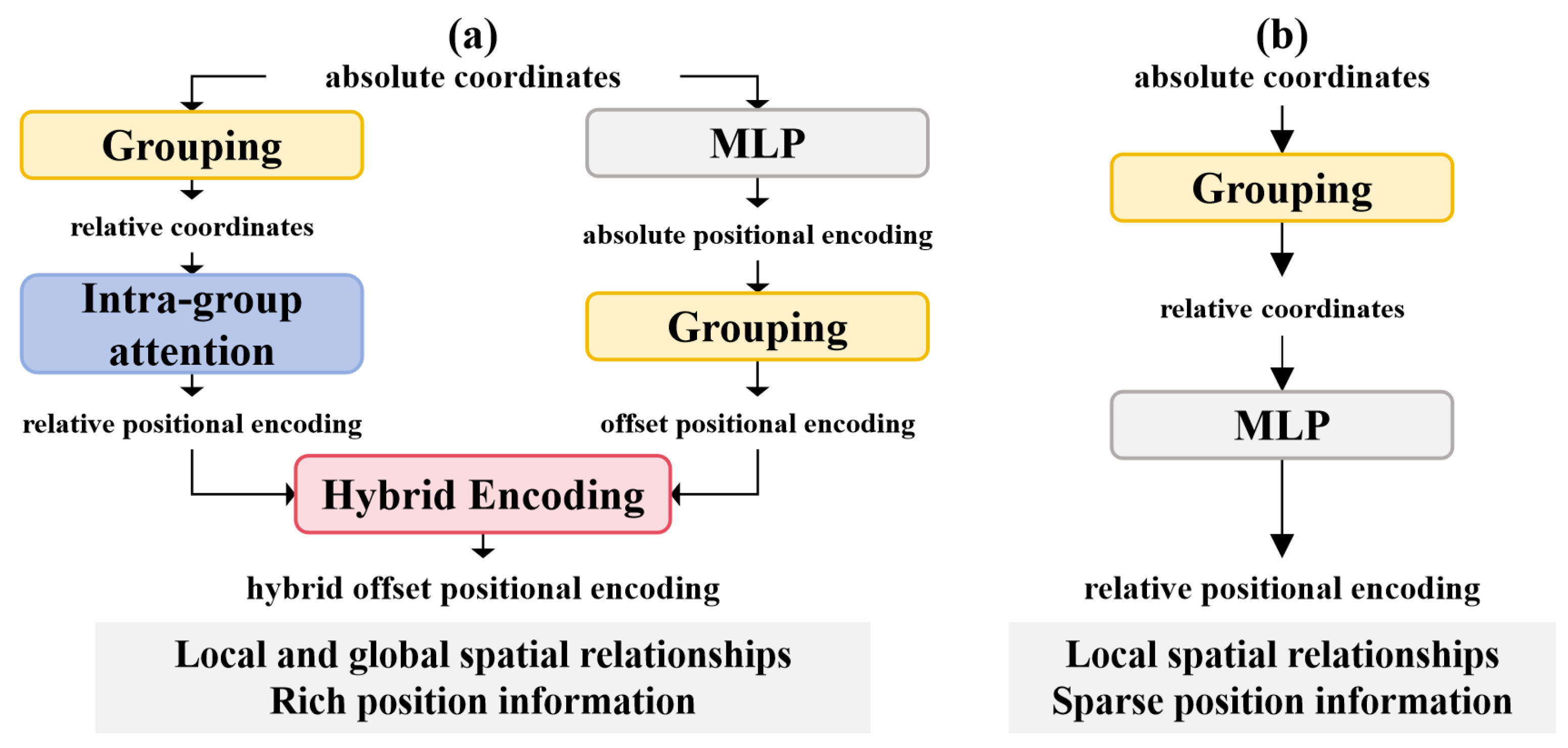
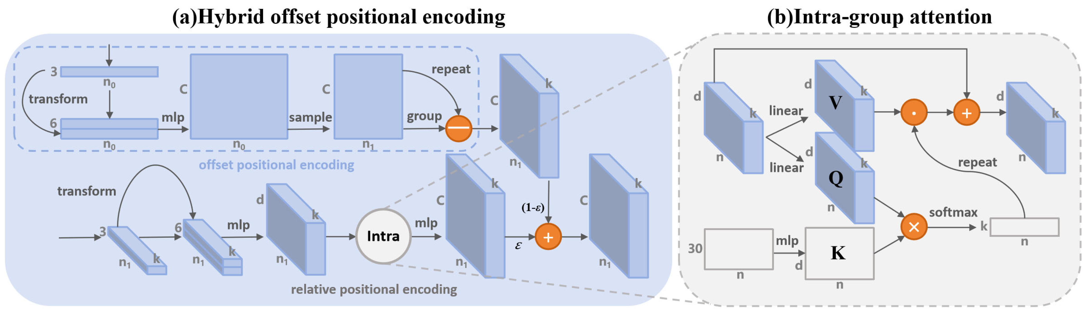
• We propose Hybrid Offset Position Encoding (HOPE), which enhances relative position encoding within the local receptive field through an attention mechanism guided by explicit structures. Additionally, we introduce offset position encoding derived from the global receptive field. These two encodings are adaptively combined, boosting the spatial awareness of the network’s deep encoder with minimal computational overhead, thereby improving performance on large-scale point cloud semantic segmentation tasks.
• We validate the effectiveness and generalizability of our module through experiments on point cloud semantic segmentation tasks across multiple large-scale datasets and baselines.

2. Related Work

2.1. Point-Based Network

Convolutional neural networks (CNNs) have achieved significant success in the field of computer vision [23,24]. However, due to the irregularity of point clouds, traditional convolutions cannot be directly applied to point cloud data. To address this, some methods, such as [25,26,27,28], voxelize the input point cloud and apply 3D convolutions. However, this approach often loses many details of the point cloud, leading to reduced performance.

To avoid these issues, many point-based networks, such as [1,2], have emerged. These networks can directly capture patterns from irregular point clouds, avoiding intermediate representations and additional preprocessing or postprocessing steps. This reduces the loss of details and simplifies the workflow. Based on PointNet and PointNet++, several works have used shared MLPs as the basic unit of the network, employing various aggregation methods and grouping strategies to extract multi-scale point cloud features [7,29,30,31,32,33,34,35]. Other works use different methods to generate effective convolutional kernels to dynamically adjust point features [4,5,6,13,14,15,16,36,37]. Some approaches also use Recurrent Neural Networks (RNNs) for semantic segmentation of point clouds to capture inherent contextual features [38,39,40,41]. Additionally, to capture the underlying shape and geometric structure of point clouds, some methods use graph networks [3,42,43,44,45].

Among these point cloud networks, most involve a local aggregation process, in which embedding local positional information can significantly enhance the network’s performance. The proposed Hybrid Offset Position Encoding (HOPE) module can more effectively improve the network’s positional awareness in deeper layers.

2.2. Attention Mechanism

The concept of the attention mechanism was first introduced in the field of neural networks [46] to allow models to focus on important parts of the input and suppress irrelevant parts. Vaswani et al. introduced a concept [47] which relies entirely on the attention mechanism for information processing and has become the standard architecture in NLP tasks, such as [48,49]. Wang et al. introduced the Non-Local Neural Network [50], which applied self-attention mechanisms to image and video processing tasks. Refs. [51,52] brought the superiority of Transformers to the visual domain. Since then, many researchers have proposed novel attention mechanisms, such as [53], which simplifies spatial attention by introducing channel attention, ref. [54], which uses 1D convolutions to simplify the process of computing channel attention, and ref. [55], which divides channels into multiple groups. Refs. [56,57] combine spatial attention and channel attention.

The application of attention mechanisms in point clouds has also gained attention, and early approaches in this field typically calculate scalar attention over global receptive fields, such as [58,59,60,61,62]. These methods require a large amount of memory because they operate on all points directly. Refs. [10,17] calculate attention maps in local receptive fields using vector attention, which effectively aggregates local features but struggles to model global contextual information. Some methods have combined local and global attention [29,60,63], but these approaches significantly increase the network’s parameters. Subsequently, ref. [18] used dense keys for nearby points and sparse keys for distant points to expand the receptive field of attention. Ref. [64] utilized a small number of self-positioning point sets to capture global features while reducing computation.

In this paper, we leverage the attention mechanism to assign different weights to different point encodings, allowing the network to focus on more important points. Unlike the previous attention mechanisms, our method differs by using explicit encoding to guide the learning of attention.

2.3. Positional Encoding

The previous section introduced related works on attention mechanisms, many of which require positional encoding as a bias term. For self-attention mechanisms, there is an inherent limitation: they cannot capture the order of input tokens. Therefore, explicit representations of positional information are especially important for Transformers, as otherwise, the model will be entirely unaffected by the sequence order [65]. For Transformers, positional encoding can be classified into two types: absolute positional encoding (APE) [47,66], and relative positional encoding (RPE) [67,68]. APE assigns a unique encoding to each position, whereas RPE encodes the relative distance between input elements.

In the point cloud domain, RPE is more commonly used because relative positions exhibit translation invariance and contain more local details [69]. Since point clouds inherently come with coordinates, some methods [10,17,70,71] generate positional encodings in a learnable manner using the relative coordinates of neighboring points. Ref. [18] discovered that the position bias learned by a simple MLP is similar between different neighboring points. To increase the diversity of the encoding, they designed a learnable quantization lookup table for relative positional encoding. Ref. [19] directly uses trigonometric functions to explicitly encode relative positions. Recently, networks such as [9,72] have used positional encoding directly as a local aggregation positional embedding process, opening new possibilities for positional embedding methods.

Compared to the aforementioned positional encoding methods, our approach combines explicit encoding in the form of attention with implicit learning of positional encodings. Additionally, we introduce a branch to compute offset positional encodings. Since this is only applied to the deeper layers of the encoder and involves fewer parameters, it provides performance improvement with minimal computational overhead. In contrast, the Stratified Transformer’s positional encoding requires dot product operations with query and key features to obtain position biases, which is not suitable for MLP-based point cloud networks. Our method, however, is applicable to a broader range of networks.

3. Rethinking Point Cloud Position Embedding

The closer the positions of two points are, the more similar their semantics are. Therefore, embedding positional information into features is an essential process in point cloud analysis. According to the form of position embedding, this paper categorizes learnable position embeddings as implicit position embeddings, and non-learnable ones as explicit position embeddings. The implicit position embeddings can be further subdivided as follows:

-

Concatenation-based position embedding, such as in works like [2,6,7,8,12,64,73].

-

Kernel-based position embedding, as seen in [4,5,13,14,15,16,74].

-

Bias-based position embedding, used in works like [9,10,17,70,71,72,75].

Explicit position embeddings are mainly represented by works like [19,20,21,22]. Position embeddings are primarily utilized in the local aggregation process within the encoder, such as in PointNet++, which performs local aggregation at the set abstraction layer. In this section, we first briefly outline the background of local aggregation and then discuss these two types of position embeddings in depth.

3.1. The Background of Local Aggregation

Assuming a 3D point cloud contains $N$ points, we can represent it as a set of $N$ points, denoted by $p\in {\mathbb{R}}^{N\times 3}$, where 3 corresponds to the three coordinates of each point. Let $f\in {\mathbb{R}}^{N\times C}$ represent the point embeddings, where $C$ is the number of channels for each point.

Before local aggregation, we typically downsample the center points and then use KNN or ball query to search for neighbors for each center point. For the $i$-th center point $p_i$, assume it has $k$ neighboring points, where the $j$-th neighbor is $p_{ij}$, with $j=\mathrm{1,2},\dots ,k$. The features of the center point and the neighboring points are denoted as $f_i$ and $f_{ij}$, respectively. Thus, the local aggregation process can be formalized as follows:

$$F_i=A_{j=1}^k\left(F_{PE}\left(f_{ij},p_{ij}\right)\right).$$

(1)

where $F_i$ represents the output feature of the center point, ${\mathcal{A}}_{j=1}^k(\cdot )$ denotes the aggregation function, which is a symmetric operator (SOP) such as max pooling, summation, etc., ${\mathcal{F}}_{PE}(\cdot )$ represents the position embedding function, which includes both implicit and explicit position embedding methods. The following sections introduce these two types of position embedding approaches.

3.2. Implicit Position Embedding

Implicit position embedding refers to embedding positions in a learnable manner, and the process is carried out implicitly within the network. In the field of point clouds, most approaches opt for implicit methods to fuse semantic features with position features because these methods are adaptable and have a simple structure. However, the shortcoming is that they tend to have poor interpretability and limited control. Below, we will introduce a few common implicit position embedding methods.

3.2.1. Concatenation-Based Position Embedding

For this type of method, the relative coordinates $\mathsf{\Delta }{p}_{ij}$ are obtained by subtracting the center point $p_i$ from the neighboring point $p_{ij}$. The relative coordinates are then concatenated with the neighbor features $f_{ij}$ and mapped to achieve position embedding (as shown in Figure 2a). This method was first applied to local aggregation by PointNet++ [2], and its general expression is:

$$h_{ij}=\varphi \left(\mathrm{c}\mathrm{o}\mathrm{n}\mathrm{c}\mathrm{a}\mathrm{t}(f_{ij},(\mathsf{\Delta }{p}_{ij}))\right)$$

(2)

where $h_{ij}$ represents the neighbor features after position modeling, and $\varphi (\cdot )$ is the mapping function, such as an MLP. In methods like PointMixer [12], the coordinates and features are simply fed into the mapping function to align the distributions of the two types of features, enhancing the expressiveness. Its formula is:

$$h_{ij}=\varphi \left(\mathrm{c}\mathrm{o}\mathrm{n}\mathrm{c}\mathrm{a}\mathrm{t}(\theta \left(f_{ij}\right),\psi (\mathsf{\Delta }{p}_{ij}))\right)$$

(3)

where $\theta (\cdot )$ and $\psi (\cdot )$ are mapping functions. Because the method concatenates the features, it leads to an imbalance in dimensions in the deeper layers of the network, resulting in insufficient positional information and thus affecting network performance. RandLA-Net [7] considers additional information such as absolute coordinates and Euclidean distances (as shown in Figure 2e), and its expression is:

$$V_{ij}=\mathrm{c}\mathrm{o}\mathrm{n}\mathrm{c}\mathrm{a}\mathrm{t}(\mathsf{\Delta }{p}_{ij},p_{ij},p_i,||p_i-p_{ij}||)$$

(4)

$$h_{ij}=\varphi \left(\mathrm{c}\mathrm{o}\mathrm{n}\mathrm{c}\mathrm{a}\mathrm{t}(\theta \left(f_{ij}\right),\psi (V_{ij}))\right)$$

(5)

where $V_{ij}$ is the explicitly constructed relational vector, and $\left|\right|\cdot \left|\right|$ denotes the Euclidean distance. This method maps the position information to the same dimension as the features, alleviating the dimensional imbalance issue, and introduces other low-level geometric relationships. However, the low-level geometric connections derived from sparse point clouds may have already been distorted, and the weights learned from these connections lack generalization.

Embedding position through concatenation has a stronger fitting capability and can better establish the relationship between relative positions and point features. However, it brings larger computational overhead and dimensional imbalance issues in deeper layers. Assuming the computational complexity of a 1 × 1 convolution or linear layer is $O{(C}_{in}\times C_{out}\times N\times k)$, the complexity of bias-based methods is $O(3\times C\times N\times k)$, while for concatenation-based methods, it is $O\left(\right(C+3)\times C\times N\times k)$, resulting in an additional complexity factor of ${\displaystyle \frac{C+3}{3}}$. As the number of encoder layers increases, the complexity ratio will rise linearly.

3.2.2. Kernel-Based Position Embedding

This method models positional information in the form of weights. For example, works like PointConv [15] and Monte Carlo convolution [74] use relative coordinates to construct convolution kernels, with the position embedding expression as follows:

$$h_{ij}=f_{ij}\odot \mathcal{W}(\mathsf{\Delta }{p}_{ij})$$

(6)

where $\mathcal{W}(\cdot )$ denotes the weight generation function. In methods like PAConv [16] and RSConv [4], a geometry construction function is introduced, incorporating additional low-level geometric information:

$$h_{ij}=f_{ij}\odot \mathcal{W}(F((\mathsf{\Delta }{p}_{ij}),f_{ij}))$$

(7)

where $F\left(\cdot \right)$ represents the geometry construction function. However, this approach is similarly unsuitable for sparse point clouds in deep networks and requires considerable computation.

Kernel-based methods adaptively adjust features through weights, akin to convolution operations. However, this approach does not directly embed position; instead, it indirectly transforms relative positions into convolution kernels to distinguish neighboring points (as shown in Figure 2b,f).

3.2.3. Bias-Based Position Embedding

Bias-based position embedding refers to learnable positional encoding. Most Transformer-based point cloud networks, such as Point Transformer [10], Point Transformer V2 [17], and ConDaFormer [70], use bias to integrate positional information (as shown in Figure 2c). These networks also use kernels to adjust features, but they decouple the vector kernel constructing local structure from the position embedding process, providing better interpretability and generally achieving improved performance. Recently, MLP-based networks like RepSurf [72], PointMetabase [9], and X-3D [75] have also adopted this method (as shown in Figure 2g). The process of bias-based position embedding can be formulated as follows:

$$h_{ij}=f_{ij}+\psi (\mathsf{\Delta }{p}_{ij})$$

(8)

where $\psi (\cdot )$ is a mapping function. By mapping relative coordinates to the same dimension as point features, this approach avoids dimensional imbalance, helping to prevent the loss of positional information in deeper network layers. However, the positional embedding generated by a simple $\psi (\cdot )$ may become diluted in deep layers, causing position embeddings between neighboring points to be overly similar.

3.3. Explicit Position Embedding

To build parameter-free networks, Point-NN [19] and Seg-NN [20] draw inspiration from the [47] by using trigonometric functions to generate fixed positional encodings (as shown in Figure 2h). The expression for their positional embedding is:

$$h_{ij}=\mathcal{E}(\mathsf{\Delta }{p}_{ij})\odot f_{ij}+\mathcal{E}(\mathsf{\Delta }{p}_{ij})$$

(9)

where $\mathcal{E}(\cdot )$ denotes the explicit encoding function. On the other hand, methods like ASSANet [21] and PosPool [22] treat relative positions as weights in the pooling operation, embedding positional information into the neighborhood features without needing any parameters (as shown in Figure 2d). Their expression is:

$$h_{ij}=\mathcal{E}(\mathsf{\Delta }{p}_{ij})\odot f_{ij}$$

(10)

Here, $\mathcal{E}(\mathsf{\Delta }{p}_{ij})$ represents the scalar components $[\mathsf{\Delta }{x}_{ij},\mathsf{\Delta }{y}_{ij},\mathsf{\Delta }{z}_{ij}]$ of $\mathsf{\Delta }{p}_{ij}$, replicated and multiplied with $f_{ij}$ across one-third of its channels.

This approach allows for effectively distinguishing between different points without adding parameters, and these methods have achieved strong performance within their respective networks. However, directly multiplying explicit encoding with features can alter the original feature values and introduce numerical instability, necessitating additional MLP layers to learn more complex nonlinear transformations.

4. Method

After rethinking traditional position embedding methods, we observe that most approaches use only a simple MLP as the mapping function to embed relative coordinates into features. Some methods attempt to incorporate additional low-level geometric features, but they overlook the issue of position information loss in sparse points in deeper network layers. Geometric features may also become distorted, making it difficult for a simple MLP to effectively integrate point positions and features (as illustrated in Figure 3).

To enhance spatial perception in deeper network layers, we propose a more flexible position encoding: Hybrid Offset Position Encoding (HOPE). To avoid a significant increase in computational complexity, we apply this encoding only to sparse points after multiple downsampling stages and use a bias-based approach to integrate position and feature information. Our position encoding calculation includes two branches: one calculates the relative position encoding (RPE), and the other calculates the offset position encoding (OPE), which are then merged. The relative position encoding is computed using an explicit structural encoding to obtain the attention matrix. The detailed process is introduced below.

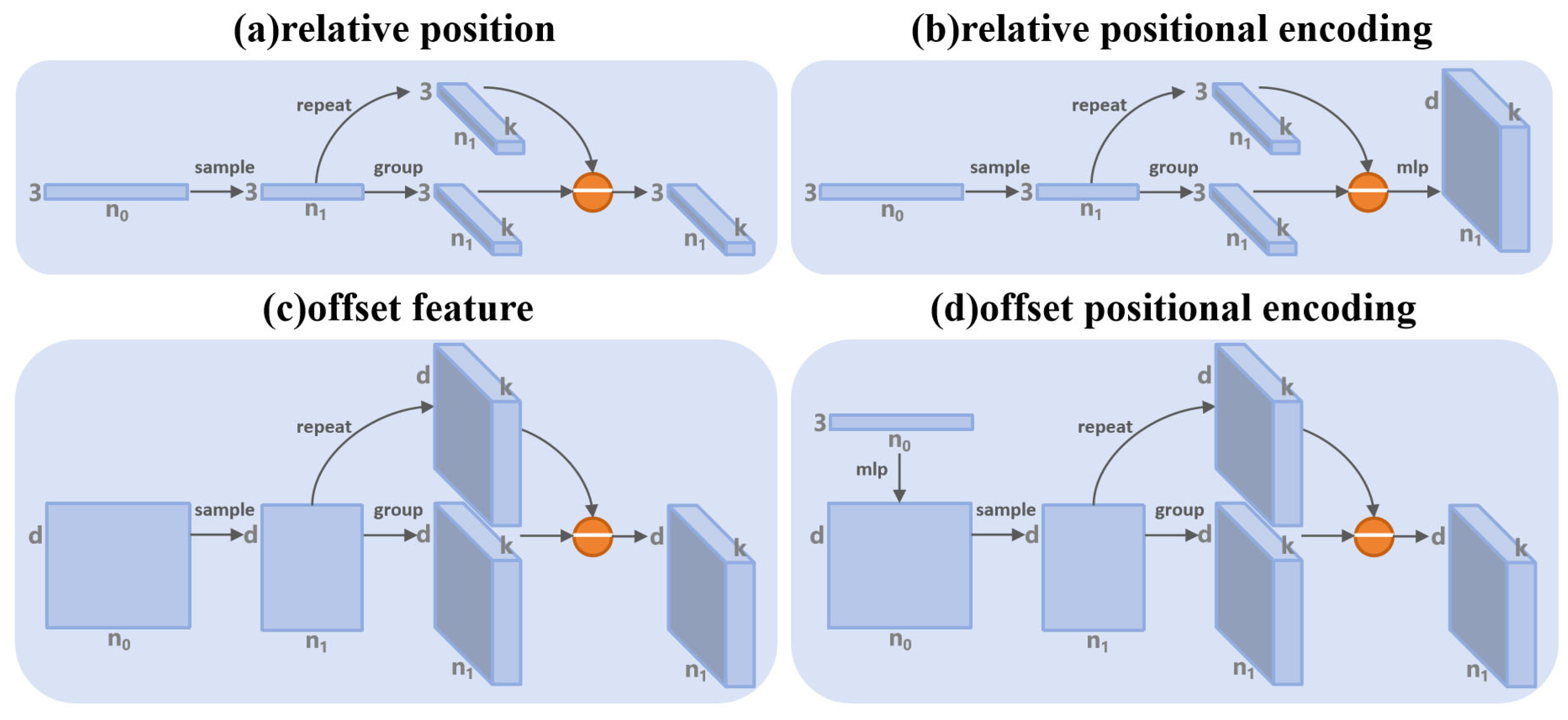
4.1. Relative Positional Encoding

To compute the relative position encoding, the relative coordinates $\mathsf{\Delta }{p}_{ij}=(\mathsf{\Delta }{x}_{ij},{\mathsf{\Delta }y}_{ij},\mathsf{\Delta }{z}_{ij})$ are typically taken as input and mapped via an MLP from three dimensions to the same dimension $\complement$ as the point feature $f_{ij}$. To enhance the model’s ability to capture spatial geometric relationships, we incorporate the spherical coordinate representation of the relative position ${\mathsf{\Delta }s}_{ij}=(r_{ij},{\theta }_{ij},{\phi }_{ij})$. Here, the radial distance $r_{ij}=\sqrt{(\mathsf{\Delta }{x}_{ij}{)}^2+({\mathsf{\Delta }y}_{ij}{)}^2+(\mathsf{\Delta }{z}_{ij}{)}^2}$, the azimuth angle $\theta =\mathrm{a}\mathrm{r}\mathrm{c}\mathrm{t}\mathrm{a}\mathrm{n}2({\mathsf{\Delta }y}_{ij},\mathsf{\Delta }{x}_{ij})$, and the polar angle $\varphi =\mathrm{a}\mathrm{r}\mathrm{c}\mathrm{c}\mathrm{o}\mathrm{s}\left({\displaystyle \frac{\mathsf{\Delta }{z}_{ij}}{r}}\right)$. We concatenate these representations and map them to an intermediate dimension $d$ to obtain $X_{ij}{\in \mathbb{R}}^{N\times k\times d}$. Before concatenation, $\mathsf{\Delta }{p}_{ij}$ and ${\mathsf{\Delta }s}_{ij}$ are linearly mapped to the feature space. The calculation can be formalized as follows:

$$X_{ij}=\varphi (\mathrm{c}\mathrm{o}\mathrm{n}\mathrm{c}\mathrm{a}\mathrm{t}(\mathrm{N}\mathrm{o}\mathrm{r}\mathrm{m}({\mathrm{W}}_p\mathsf{\Delta }{p}_{ij}),\mathrm{N}\mathrm{o}\mathrm{r}\mathrm{m}({\mathrm{W}}_s{\mathsf{\Delta }s}_{ij})))$$

(11)

where $\varphi$ denotes an MLP, ${\mathrm{W}}_p$ and ${\mathrm{W}}_s$ are linear layers, and $\mathrm{N}\mathrm{o}\mathrm{r}\mathrm{m}$ represents a normalization layer, typically batch normalization. $X_{ij}$ can be seen as an embedding enriched with position features.

We recognize that directly adding low-level geometric information may be beneficial in shallow encoding layers, but in deeper layers with sparse points, geometric connections may become distorted due to the presence of noisy points deviating from the local structure. Therefore, we designed an intra-group attention module to diminish the influence of points that significantly deviate from the local structure. Inspired by [75], we utilize explicit structural encoding as a key to compare with the query, and, considering the symmetry in Pointhop [76], we use it as the explicit structure generation function. The explicit encoding is calculated as follows:

$$E_i=\mathcal{E}(\mathsf{\Delta }{p}_{ij},p_i)$$

(12)

where $E_i{\in \mathbb{R}}^{N\times 30}$ represents the explicit encoding matrix. $\mathcal{E}(\cdot )$ denotes the explicit encoding function. $E_i$ includes centroid coordinates in eight quadrants within the neighborhood of the central point and additional information to encode the local structure. Details on the calculation process can be found in [76].

Next, intra-group attention can be formulated as follows:

$$q={\mathrm{W}}_q{X}_{ij}$$

(13)

$$k={\varphi }_k{(E}_i)$$

(14)

$$v={\mathrm{W}}_v{X}_{ij}$$

(15)

$$\mathrm{IntraAtten}(X_{ij},E_i)=\mathcal{R}(\mathrm{softmax}\left(q\cdot k^T\right))\odot v$$

(16)

where ${\mathrm{W}}_q$ and ${\mathrm{W}}_v$ are linear layers, ${\varphi }_k$ is an MLP for nonlinearly transforming $E_i$ and reshaping it to $[N\times d]$ to match the shape of $q$ and $v$. $\mathcal{R}(\cdot )$ is a replication operator that duplicates the attention matrix $d$ times, and $\odot$ represents element-wise multiplication. This gives the enhanced geometric structure embedding $Y_{ij}$:

$$Y_{ij}=\mathrm{IntraAtten}\left(X_{ij},E_i\right)+X_{ij}$$

(17)

Each channel of every point in $Y_{ij}{\in \mathbb{R}}^{N\times k\times d}$ is assigned a weight to enhance important features. Then, we use an MLP to align $Y_{ij}$ with the feature space of point features $f_{ij}{\in \mathbb{R}}^{N\times k\times C}$ and add them:

$$R_{ij}=\psi \left(Y_{ij}\right)$$

(18)

$$h_{ij}=f_{ij}+R_{ij}$$

(19)

where $\psi$ denotes an MLP, $R_{ij}{\in \mathbb{R}}^{N\times k\times C}$ represents the relative position encoding, and $h_{ij}$ is the feature of the neighboring point after position embedding.

In addition to computing the relative position encoding $R_{ij}$, we propose an additional position encoding to compute extra biases, further enhancing geometric position information in deeper layers. Next, we introduce the design and calculation process of the offset position encoding.

4.2. Offset Positional Encoding

First, we revisit the calculation process for relative positions, which starts by using the point coordinates $P_i{\in \mathbb{R}}^{N_0\times 3}$ from the previous layer, downsampled to the center points $p_i{\in \mathbb{R}}^{N\times 3}$ of the current layer. $P_i$ serves as the support points, and $p_i$ as the query points, for grouping operations to obtain $p_{ij}{\in \mathbb{R}}^{N\times k\times 3}$, typically using KNN or ball query. The coordinates of each center point $p_i$, duplicated k times, are subtracted from the grouped points $p_{ij}$ to obtain the positional difference of neighboring points, also known as the relative position $\mathsf{\Delta }{p}_{ij}$ (as shown in Figure 4a). Some approaches, such as DGCNN [3] and DeepGCN [43], attempt to compute feature differences between neighboring points in high-dimensional space using a similar approach, which helps in constructing a directed graph and is also referred to as edge features or offset features (as shown in Figure 4c). These methods fall under graph-based point cloud networks, which leverage offset features to more effectively capture underlying shapes and geometric structures in point clouds. Inspired by these networks, we adapted this method to positional encoding.

Unlike the relative positional encoding calculation (as shown in Figure 4b), we use the unsampled absolute positions $P_i$ as input, initially modeling them as high-dimensional absolute positional encodings. Then, we retrieve the high-dimensional encodings of neighboring and center points through indexing, and subsequently calculate the difference between their encoding values to obtain the offset positional encoding (as shown in Figure 4d). In practice, we take the absolute position $P_i$ and its corresponding spherical coordinates $S_i$, linearly map and concatenate them as input. The calculation process is formulated as follows:

$$a_i={\varphi }_{pre}(\mathrm{c}\mathrm{o}\mathrm{n}\mathrm{c}\mathrm{a}\mathrm{t}(\mathrm{N}\mathrm{o}\mathrm{r}\mathrm{m}({\mathrm{W}}_P{P}_i),\mathrm{N}\mathrm{o}\mathrm{r}\mathrm{m}({\mathrm{W}}_S{S}_i)))$$

(20)

$$A_{ij}=\mathcal{G}\left(\mathcal{D}\left(a_{ij}\right)\right)$$

(21)

$$A_{ii}=\mathcal{R}\left(\mathcal{D}\left(a_{ij}\right)\right)$$

(22)

$$O_{ij}=A_{ii}-A_{ij}$$

(23)

where ${\varphi }_{pre}$ denotes a MLP, $\mathcal{D}(\cdot )$, $\mathcal{G}(\cdot )$ and $\mathcal{R}(\cdot )$ represent downsampling, grouping, and replication operations, respectively. $a_i{\in \mathbb{R}}^{N_0\times C}$ represents the absolute positional encoding of all points, $A_{ij}{\in \mathbb{R}}^{N\times k\times C}$ and $A_{ii}{\in \mathbb{R}}^{N\times k\times C}$ are the grouped absolute positional encodings and the center point’s absolute positional encoding duplicated $k$ times. $O_{ij}{\in \mathbb{R}}^{N\times k\times C}$ denotes the offset positional encoding.

We argue that $O_{ij}$ and $R_{ij}$ are not equivalent, as the former performs encoding based on absolute coordinates, similar to PointNet [1], by applying a shared MLP across the entire point cloud, capturing the overall point cloud characteristics. After computing differences, the global response in the feature space transforms into a local response, avoiding conflicts with $R_{ij}$. Meanwhile, $R_{ij}$ directly captures local patterns within the local space.

Additionally, assuming the same number of MLP layers and 3D Cartesian coordinates as input, the computational complexity of $O_{ij}$ is generally lower than that of $R_{ij}$. When the MLP has a single layer, the complexity of $O_{ij}$ is $O(3\times C\times N_0)$, while that of $R_{ij}$ is $O(3\times C\times N\times k)$. The ratio of complexities is ${\displaystyle \frac{N_0}{N\times k}}$. Let $\alpha$ represent the downsampling rate, then this ratio can be written as ${\displaystyle \frac{N\times \alpha }{N\times k}}$, simplifying to ${\displaystyle \frac{\alpha }{k}}$. In most networks, the downsampling rate $\alpha$ is far less than the number of neighboring points $k$. For example, in the set abstraction layers of [2,8,9], $\alpha =4$ and $k=32$, making the computational complexity of $O_{ij}$ one-eighth that of $R_{ij}$. Hence, adding this additional branch does not impose a significant computational burden.

4.3. Hybrid Encoding

After calculating $O_{ij}$ and $R_{ij}$, there are several ways to combine them: 1. concatenation, 2. addition, 3. subtraction, and 4. multiplication. Since concatenation results in a channel dimension of $2C$, which would require mapping back to $C$ dimensions and consume substantial memory, this option can be disregarded. Based on experimental results (see Section 5.2), among the remaining three methods, addition balanced computational cost and performance best. Additionally, we introduced a learnable parameter $\epsilon$ as an adaptive weight to control the balance of $O_{ij}$ and $R_{ij}$ across layers. The final position encoding process is formulated as follows:

$$h_{ij}=f_{ij}+{\epsilon \cdot R}_{ij}+{(1-\epsilon )\cdot O}_{ij}$$

(24)

This allows the ratio of $O_{ij}$ and $R_{ij}$ to be adaptively adjusted across different layers.

5. Experiments

To demonstrate the effectiveness of HOPE, we evaluated it on two downstream tasks: large-scale indoor semantic segmentation and outdoor semantic segmentation. We also embedded HOPE into several classic models to prove its applicability. Additionally, we designed a series of ablation experiments to verify the effectiveness of each component of HOPE. All experiments were conducted on a single Nvidia GeForce RTX 4090-D GPU with 24GB of memory and an Intel i9-14900K CPU.

5.1. Large-Scale Point Cloud Semantic Segmentation

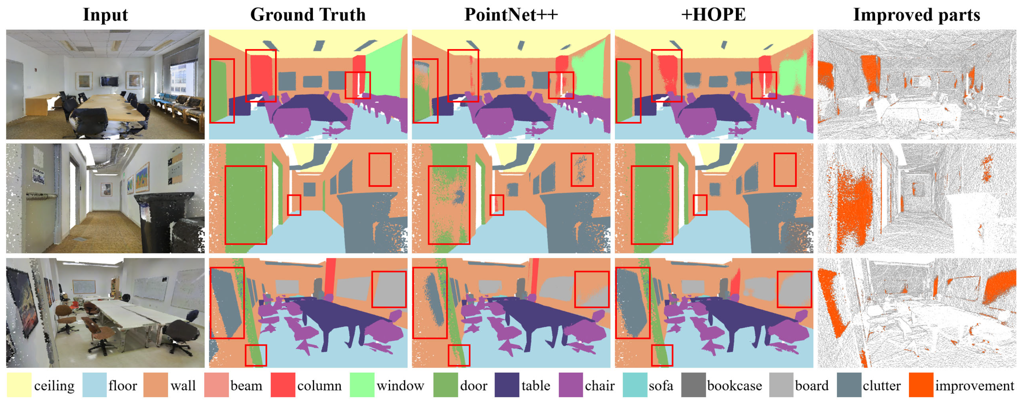
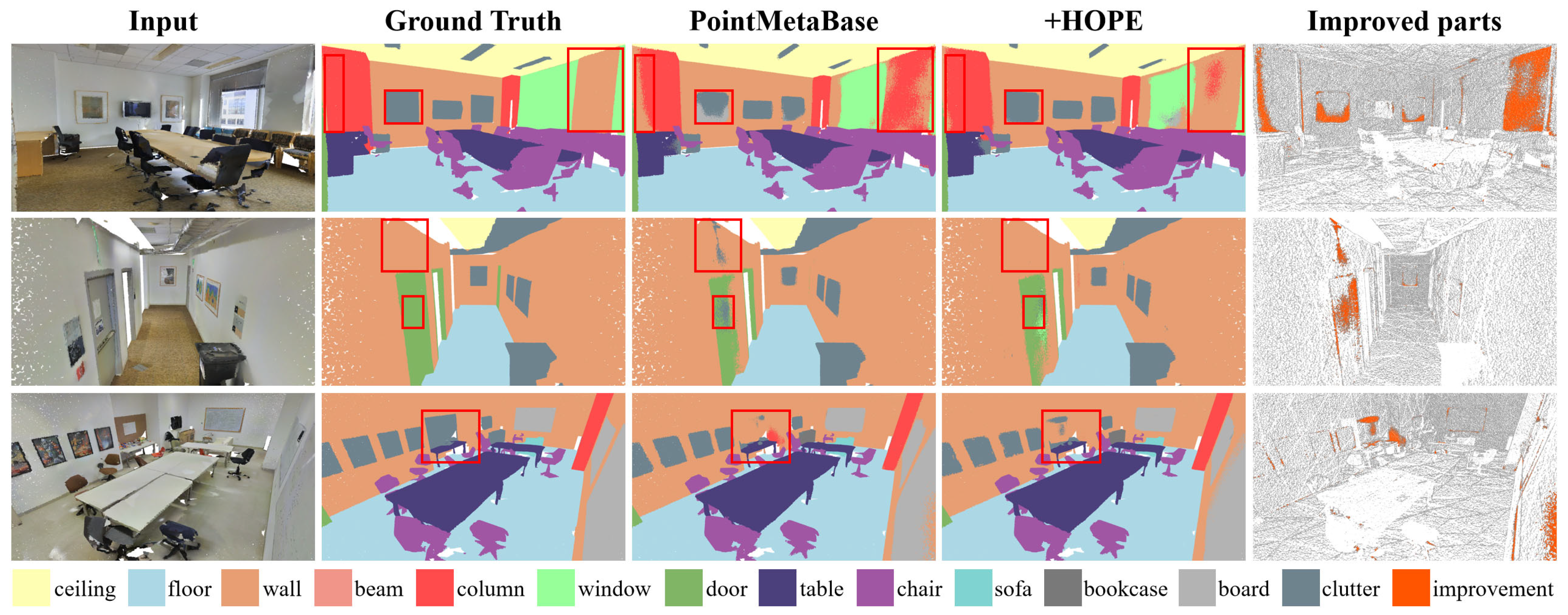
5.1.1. Evaluation on S3DIS

S3DIS [77] is a benchmark dataset released by Stanford University for 3D indoor scene understanding, containing point cloud data from six different buildings with a total area exceeding 6000 square meters. The buildings include various room types such as conference rooms, lounges, offices, etc., covering a wide range of common indoor scenes. The dataset was generated using 3D scanners, with the captured point clouds having high density and resolution, recording 3D coordinates and RGB color information for each point. Each scene’s point cloud not only contains geometric information but is also carefully annotated with semantic labels. Specifically, the dataset includes 13 common indoor object labels, such as walls, floors, tables, chairs, doors, bookshelves, etc.

We evaluated our HOPE implementation using two evaluation methods: one using area-5 as the test scene with the rest for training, and the other using standard six-fold cross-validation. We implemented HOPE on PointNet++ [2] and PointMetaBase [9] to validate its effectiveness. The version of PointNet++* used here is based on the open-source code from PointNeXt [8], which has undergone training strategy adjustments and performs better performance. During training, we fixed the input size to 24,000 points, set training epochs to 100, and batch size to 16. We used CrossEntropy loss, AdamW optimizer, an initial learning rate of 0.01, and cosine decay for optimization, keeping these configurations consistent with the official ones.

After implementing HOPE on both PointNet++ and PointMetaBase, we achieved a 2.1%, 1.3%, and 1.0% improvement in mIoU, and a 0.6%, 0.3%, and 0.4% improvement in OA in the area-5 task (as shown in

Table 1. Quantitative comparison of different methods on S3DIS area-5.

Method	S3DIS Area-5			FLOPs (G)	Params. (M)	Throughput (ins./s)
	mIoU (%)	mAcc (%)	OA (%)
PointNet++ [2]	53.5	-	83.0	7.2	1.0	186
ASSANet [21]	63.0	-	-	2.5	2.4	-
Point Transformer [10]	70.4	76.5	90.8	5.6	7.8	34
PointNeXt-XL [8]	71.1	77.5	91.0	84.8	41.0	46
PointVector-XL [73]	72.3	78.1	91.0	58.5	24.1	40
ConDaFormer [70]	72.6	-	91.6	-	-	-
PointNAT [71]	72.8	-	91.5	12.9	24.9	135
PointNet++* [2]	63.6	70.2	88.3	7.2	1.0	186
+HOPE	65.7 (+2.1)	72.2 (+2.0)	88.9 (+0.6)	6.9	1.1	185
PointNeXt-L [8]	69.5	76.1	90.1	15.2	7.1	115
+HOPE	71.2 (+1.7)	77.5 (+1.4)	90.7 (+0.6)	14.8	7.2	117
PointMetaBase-L [9]	69.7	75.6	90.6	2.0	2.7	187
+HOPE	71.0 (+1.3)	77.1 (+1.5)	90.9 (+0.3)	2.2	2.8	182
PointMetaBase-XL [9]	71.6	77.9	90.6	9.2	15.3	104
+HOPE	72.6 (+1.0)	78.9 (+1.0)	91.0 (+0.4)	9.6	15.4	100

). The increase in parameters and FLOPs was minimal. Notably, by switching from concatenation to a bias-based embedding in PointNet++, we reduced some of the FLOPs. Figure 5 and Figure 6 display the visualization results, showing that after adding HOPE, both baselines had increased regions of correct classification. For instance, in the first rows of Figure 5, the classification of the “column” category was more accurate, thanks to the richer positional information in the sparse points. We also validated the effectiveness of HOPE in 6-fold, as shown in

Table 2. Quantitative comparison of different methods on S3DIS 6-fold. Bold indicates the best result.

Method	mIoU	OA	Ceil.	Floor	Wall	Beam	col.	Wind.	Door	Table	Chair	Sofa	Book.	Board	Clut.
PointNet [1]	47.6	78.6	88.0	88.7	69.3	42.4	23.1	47.5	51.6	54.1	42.0	9.6	38.2	29.4	35.2
DGCNN [3]	55.5	84.5	93.2	95.9	72.8	54.6	32.2	56.2	50.7	62.8	63.4	22.7	38.2	32.5	46.8
PointCNN [6]	65.4	88.1	94.2	97.3	75.8	63.3	51.7	58.4	57.2	71.6	69.1	39.1	61.2	52.2	58.6
KPConv [5]	70.6	-	93.6	92.4	83.1	63.9	54.3	66.1	76.6	57.8	64.0	69.3	74.9	61.3	60.3
RandLA-Net [7]	70.0	88.0	93.1	96.1	80.6	62.4	48.0	64.4	69.4	69.4	76.4	60.0	64.2	65.9	60.1
Point Transformer [10]	73.5	90.2	94.3	97.5	84.7	55.6	58.1	66.1	78.2	77.6	74.1	67.3	71.2	65.7	64.8
SPTransformer [78]	76.0	-	93.9	96.3	84.3	71.4	61.3	70.1	78.2	84.6	74.1	67.8	77.1	63.6	65.0
PointNAT [71]	77.8	91.7	94.7	97.9	85.8	65.3	63.5	72.8	79.7	77.3	81.7	78.4	76.8	72.1	65.3
PointNet++* [2]	68.1	87.6	93.5	94.0	81.4	54.2	48.8	59.8	74.0	71.6	67.8	56.6	64.3	62.7	56.5
+HOPE	70.6 (+2.5)	88.6 (+1.0)	92.8	93.9	83.7	50.7	56.6	61.4	81.7	74.5	66.4	58.2	67.6	66.6	63.5
PointMetaBase-L [9]	75.6	90.6	94.9	97.6	85.4	68.6	62.0	66.8	80.1	76.5	71.1	77.3	69.5	68.6	64.8
+HOPE	76.7 (+1.1)	91.1 (+0.5)	95.0	97.2	84.3	65.2	64.2	67.5	81.2	79.6	75.8	80.2	72.1	69.2	65.5

, with significant improvements in categories such as column, door, and table.

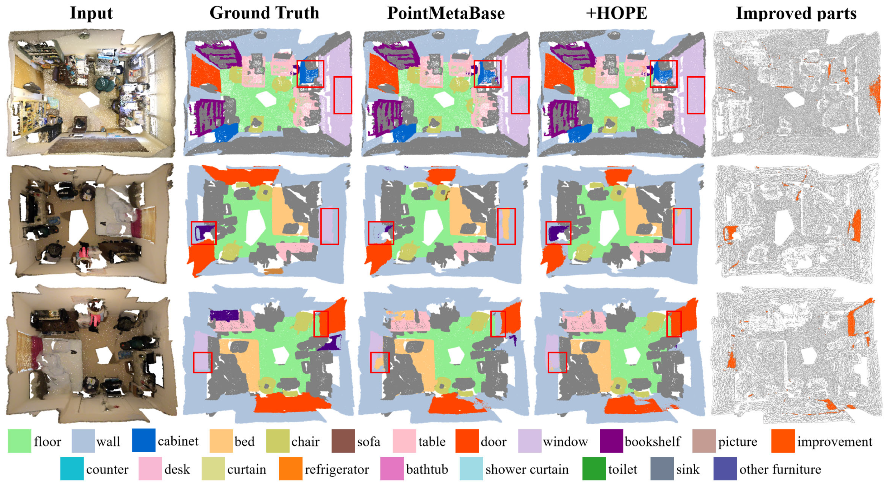
5.1.2. Evaluation on ScanNet

ScanNet [79] includes over 1500 different indoor scene scans, covering offices, bedrooms, living rooms, etc. Each scene is generated by scanning with an RGB-D sensor, combining RGB images with depth data. The dataset provides detailed semantic labels, including 20 common object categories, such as tables, chairs, sofas, etc.

We followed the standard training set of 1201 and validation set of 312. The AdamW optimizer was used with an initial learning rate of 0.001 and cosine decay for optimization.

As shown in

Table 3. Quantitative comparison of different methods on ScanNet.

Method	ScanNet	FLOPs (G)	Params. (M)
	mIoU (%)
PointCNN [6]	45.8	-	0.6
PointNet++ [2]	53.5	7.2	1.0
KPConv [5]	68.4	-	15.0
Point Transformer [10]	70.6	5.6	7.8
RepSurf [72]	70.0	-	-
PointNeXt-XL [8]	71.5	84.8	41.0
PointMetaBase-XL [9]	71.8	9.2	15.3
PointNet++* [2]	57.2	7.2	1.0
+HOPE	58.7 (+1.5)	6.9	1.1
PointMetaBase.-L [9]	71.0	2.0	2.7
+HOPE	71.6 (+0.6)	2.2	2.8

, adding HOPE to PointNet++* and PointMetaBase-L improved performance with only a slight increase in Param. and FLOPs. Figure 7 shows the visualization results for PointMetaBase-L, where the “improved parts” section highlights areas where errors in wall classification were corrected, thanks to the network learning more robust features.

5.1.3. Evaluation on Toronto3D

Toronto3D [80] is obtained through vehicle-mounted MLS systems, sourced from a street scene in Toronto, Canada, approximately one kilometer long. It includes four regions, each covering about 250 m, and is suitable for outdoor road-level 3D point cloud semantic segmentation tasks. The dataset contains labels for different categories, such as buildings, roads, vehicles, vegetation, etc. In addition to labels, each point includes 3D coordinates, RGB, intensity, and other information.

Since RandLA-Net [7] is efficient and simple for outdoor data, we incorporated HOPE into its network structure to evaluate its effectiveness. RandLA-Net represents the official implementation, while RandLA-Net* represents the results of our reproduction. We implemented HOPE on RandLA-Net*. During network training, 65,536 points were fed into the network, with a batch size of 4 and a maximum of 100 training epochs. The Adam optimizer was used to optimize the loss function, with an initial learning rate of 0.01. Following [80], we used Region 2 as the test set and the remaining regions as the training set.

As shown in

Table 4. Quantitative comparison of different methods on Toronto3. Bold indicates the best result.

Method	OA (%)	mIoU (%)	Road	Road mrk.	Natural	Buil.	Util.line	Pole	Car	Fence
ResDLPS-Net [81]	96.5	80.3	95.8	59.8	96.1	91.0	86.8	79.9	89.4	43.3
RandLA-Net [7]	94.4	81.8	96.7	64.2	96.9	94.2	88.0	77.8	93.4	42.9
BAF-LAC [82]	95.2	82.2	96.6	64.7	96.4	92.8	86.1	83.9	93.7	43.5
BAAF-Net [35]	94.2	81.2	96.8	67.3	96.8	92.2	86.8	82.3	93.1	34.0
LEARD-Net [83]	97.3	82.2	97.1	65.2	96.9	92.8	87.4	78.6	94.5	45.2
NeiEA-Net [84]	97.0	80.9	97.1	66.9	97.3	93.0	87.3	83.4	93.4	43.1
SFL-Net [85]	97.6	81.9	97.7	70.7	95.8	91.7	87.4	78.8	92.3	40.8
RandLA-Net* [7]	94.8	81.2	95.3	66.6	96.8	92.6	86.7	85.6	85.5	40.1
+HOPE	96.0 (+1.2)	82.6 (+1.4)	95.9	58.3	98.0	95.5	89.4	85.1	94.3	44.6

, after adding HOPE to the last two encoder layers of RandLA-Net, we observed performance improvements in most classes. This is due to HOPE capturing more detailed features in the deeper layers. Figure 8 also shows visual comparisons, where our method demonstrates higher accuracy in recognizing the “natural” and “fence” categories.

5.2. Ablation Experiments

5.2.1. Ablation of HOPE’s Internal Modules

HOPE includes two branches: relative position encoding (RPE) and offset position encoding (OPE). The RPE computation process also incorporates spherical coordinates (Sphere) and intra-group attention (IntraAtten.). We present the ablation results of HOPE’s internal modules on the PointNet++ and PointMetaBase baselines in

Table 5. Ablation of HOPE internal modules.

ID	Module				mIoU
	$+$RPE	$+$Sphere	$+$Intra Atten.	$+$OPE	PointNet++	PointMeta.-L
A1					63.6	69.7
A2				$\surd$	63.2	69.1
A3	$\surd$				64.0	69.7
A4	$\surd$	$\surd$			64.1	70.0
A5	$\surd$	$\surd$	$\surd$		64.8	70.5
A6	$\surd$	$\surd$	$\surd$	$\surd$	65.7	71.0

, using mIoU as the evaluation metric.

In Experiment A2, we only added OPE without RPE, and we observed a slight decrease in the performance of both baselines. We hypothesize that this is because OPE has a much smaller computational cost compared to RPE, resulting in weaker fitting capabilities. Experiment A3 shows that embedding based only on the bias improves PointNet++ performance, while PointMetaBase’s original implementation already uses RPE, so there was no performance change. Experiments A4 and A5 reflect the effectiveness of adding spherical coordinates and intra-group attention. In Experiment A6, combining RPE and OPE resulted in the best performance. From this, we can conclude that modeling relative positional relationships in a local coordinate system is essential, while modeling difference encoding in an absolute coordinate system can only serve as supplementary information. Furthermore, the balance and fusion method between the two are also key factors influencing performance. We will next present the ablation experiment of the fusion methods.

5.2.2. Ablation of Hybrid Encoding

We recorded the performance of RPE and OPE under different hybrid encoding methods (as shown in

Table 6. Ablation of hybrid encoding.

ID	The Method of Fusion	mIoU
		PointNet++	PointMeta.-L
B1	$\mathrm{RPE}*+$ OPE	65.3	70.6
B2	$\mathrm{RPE}*-$ OPE	63.9	69.3
B3	$\mathrm{RPE}*\odot$OPE	63.5	69.8
B4	$(\epsilon$$)\mathrm{RPE}*+$$(1-\epsilon$)OPE	65.7	71.0

). In the table, RPE* indicates that both spherical coordinates and intra-group attention have been included. From the table, it can be seen that addition and adaptive addition (experiments B1, B4) yield better results, likely because the feature distributions are similar. Element-wise subtraction weakens the original information, while multiplication is generally used when one of the components represents weights. Thus, multiplying OPE and RPE disrupts the feature information between them.

5.2.3. Complexity Analysis

Our goal is to avoid significant computational overhead. Therefore, we refrain from using overly complex structures. We provide the computational cost and throughput of the HOPE modules in

Table 7. Comparison of complexity for different components.

ID	Module	FLOPs (G)	Params. (M)	Throughput (ins./s)
C1	PointMeta.-L + RPE	1.98	2.74	189
C2	PointMeta.-L + RPE + Sphere	2.01	2.74	189
C3	PointMeta.-L + RPE + Sphere + IntraAtten.	2.20	2.77	187
C4	PointMeta.-L + RPE + Sphere + IntraAtten. + OPE	2.23	2.79	182

for reference. As seen in the table, the main computational burden, in terms of FLOPs, is observed in the intra-group attention module (C3). This is due to the introduction of an intermediate dimension. However, considering the performance contribution of this module, it may be retained. The addition of OPE primarily reduces the network throughput, likely due to operations that increase memory access, such as grouping and subtracting high-dimensional absolute position encodings. This results in a decrease in the floating-point operations per second (FLOPS), leading to an increase in the ratio of FLOPs to FLOPS. Although the addition of HOPE increases the overall computational load, its cost-effectiveness is significant. For example, the performance of PointMetaBase-L with HOPE on the ScanNet dataset (71.6) is nearly on par with PointMetaBase-XL, which has significantly more parameters and FLOPs (71.8).

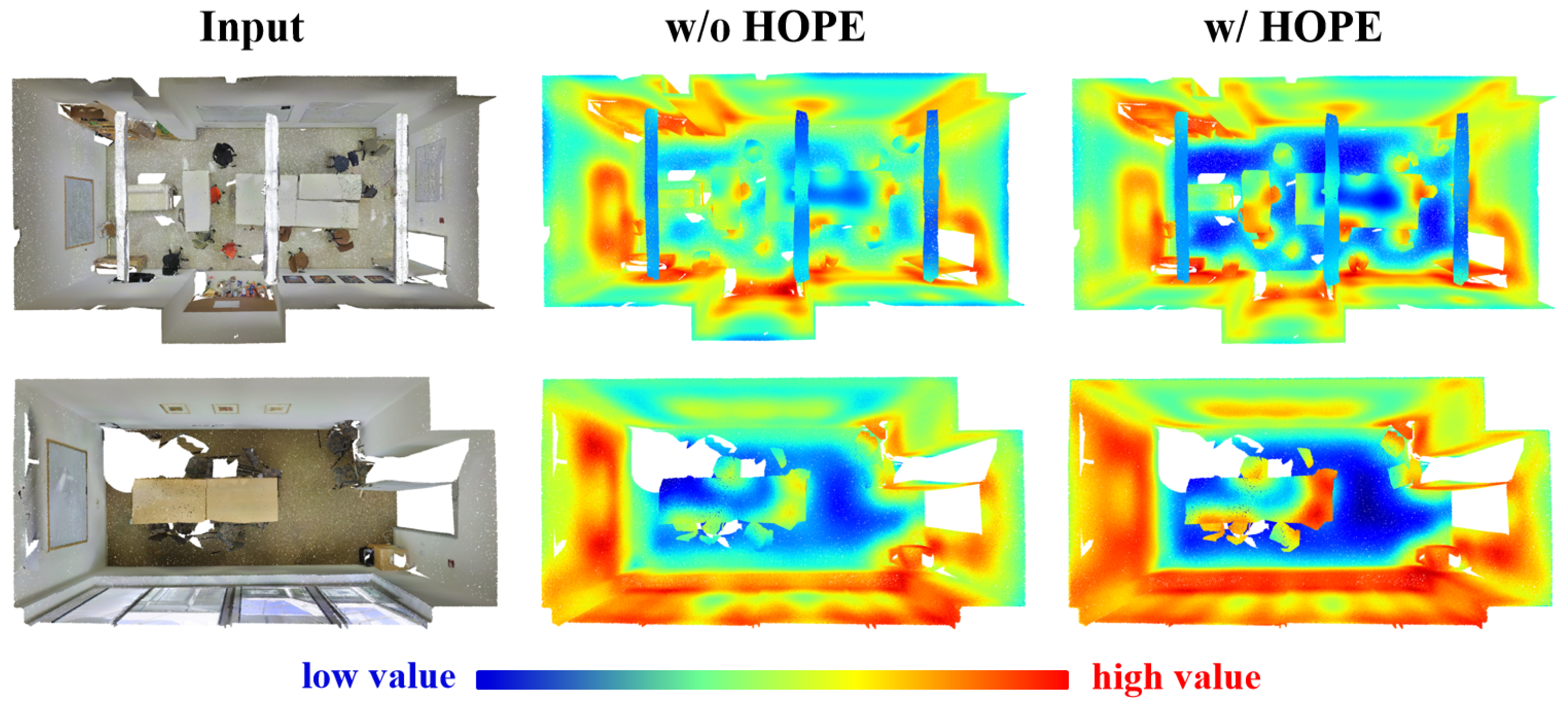
5.2.4. Heatmap Analysis

We visualized the feature maps output by the deep encoder in the cases with and without HOPE (using lightweight MLP and HOPE to generate position encoding) through heatmaps. The heatmaps were generated by interpolating the deep encoder’s output features back to the original point count. Then, the mean value of all channels for each point was calculated, and the color was assigned based on the mean value. Higher values are represented in red, while lower values are represented in blue. Patterns with high-value points are given more attention by the network. As shown in Figure 9, in the heatmap based on HOPE, the feature values are sparser, and high-value points are mostly located at edges and corners. This suggests that after adding HOPE, the network focuses more on robust and representative features. It also indicates that the model can effectively filter out noise, which may be attributed to the intra-group attention module. In contrast, the high-value points in the original network are more densely located, with boundary blur and excessive diffusion. This shows that the network, which only uses simple MLP for deep embedding, lacks sufficient discrimination ability and extracts more redundant features.

6. Discussion

In this section, we analyze in detail why HOPE works. The initial information of input point clouds typically consists of coordinate values. Current popular point cloud networks directly extract point features from the coordinate set through encoders. However, the high-level features captured by deep encoders are often more abstract, potentially weakening the lowest-level positional information. Therefore, deep encoders require stronger spatial perception and modeling capabilities.

Additionally, one limitation of existing positional encoding methods is their tendency to map relative positions in a local coordinate system from low-dimensional (3D) space to high-dimensional space. While this approach enhances the perception of local geometric connections, it fails to encode global contextual information. In contrast, HOPE not only enhances relative positional embeddings (RPE) with intra-group attention modules but also supplements them with global information through offset position encoding (OPE).

More specifically, RPE modeled under relative coordinates tends to excel at recognizing local patterns due to its symmetrical advantages in constructing point-pair relationships. However, it overlooks the positions of points in the global coordinate system and their connections with other regions, limiting its ability to model the overall geometric shape of the point cloud. On the other hand, OPE models global spatial relationships in absolute coordinates, compensating for the shortcomings of RPE.

By adaptively blending RPE and OPE through enhanced attention mechanisms and applying them to sparse points in deeper network layers where richer positional information is crucial, the network’s recognition performance can be improved with only a slight increase in computational cost.

7. Conclusions

In this paper, we propose Hybrid Offset Position Encoding (HOPE) to enhance the spatial perception ability of the deep encoders. HOPE combines the more refined relative position encoding (RPE) and offset position encoding (OPE) with an adaptive hybrid approach, addressing the sparse position feature issue in deep layers. Experimental results on multiple large-scale point cloud datasets show that our method effectively alleviates the sparsity of position information in deep layers, helping the network capture more robust features in deeper layers and thus improving the performance of the baseline models. In addition, we conducted ablation studies to demonstrate the effectiveness of each module within HOPE and to analyze different methods of hybrid encoding. Complexity analysis and heatmap analysis further validated HOPE’s low computational cost and its enhanced capability for deep encoder feature recognition. We hope our approach can provide a new perspective for the research direction of positional encoding.

References

1. Qi, C.R.; Su, H.; Mo, K.; Guibas, L.J. Pointnet: Deep learning on point sets for 3d classification and segmentation. In Proceedings of the IEEE Conference on Computer Vision and Pattern Recognition 2017, Honolulu, HI, USA, 21–26 July 2017; pp. 652–660. [Google Scholar]
2. Qi, C.R.; Yi, L.; Su, H.; Guibas, L.J. Pointnet++: Deep hierarchical feature learning on point sets in a metric space. Adv. Neural Inf. Process. Syst. 2017, 30. [Google Scholar]
3. Wang, Y.; Sun, Y.; Liu, Z.; Sarma, S.E.; Bronstein, M.M.; Solomon, J.M. Dynamic graph cnn for learning on point clouds. ACM Trans. Graph. (Tog) 2019, 38, 1–12. [Google Scholar] [CrossRef]
4. Liu, Y.; Fan, B.; Xiang, S.; Pan, C. Relation-shape convolutional neural network for point cloud analysis. In Proceedings of the IEEE/CVF Conference on Computer Vision and Pattern Recognition 2019, Long Beach, CA, USA, 15–20 June 2019; pp. 8895–8904. [Google Scholar]
5. Thomas, H.; Qi, C.R.; Deschaud, J.E.; Marcotegui, B.; Goulette, F.; Guibas, L.J. Kpconv: Flexible and deformable convolution for point clouds. In Proceedings of the IEEE/CVF International Conference on Computer Vision 2019, Seoul, Republic of Korea, 27 October–2 November 2019; pp. 6411–6420. [Google Scholar]
6. Li, Y.; Bu, R.; Sun, M.; Wu, W.; Di, X.; Chen, B. Pointcnn: Convolution on x-transformed points. Adv. Neural Inf. Process. Syst. 2018, 31. [Google Scholar]
7. Hu, Q.; Yang, B.; Xie, L.; Rosa, S.; Guo, Y.; Wang, Z.; Trigoni, N.; Markham, A. Randla-net: Efficient semantic segmentation of large-scale point clouds. In Proceedings of the IEEE/CVF Conference on Computer Vision and Pattern Recognition 2020, Seattle, WA, USA, 13–19 June 2020; pp. 11108–11117. [Google Scholar]
8. Qian, G.; Li, Y.; Peng, H.; Mai, J.; Hammoud, H.; Elhoseiny, M.; Ghanem, B. Pointnext: Revisiting pointnet++ with improved training and scaling strategies. Adv. Neural Inf. Process. Syst. 2022, 35, 23192–23204. [Google Scholar]
9. Lin, H.; Zheng, X.; Li, L.; Chao, F.; Wang, S.; Wang, Y.; Tian, Y.; Ji, R. Meta architecture for point cloud analysis. In Proceedings of the IEEE/CVF Conference on Computer Vision and Pattern Recognition 2023, Vancouver, BC, Canada, 17–24 June 2023; pp. 17682–17691. [Google Scholar]
10. Zhao, H.; Jiang, L.; Jia, J.; Torr, P.H.; Koltun, V. Point transformer. In Proceedings of the IEEE/CVF International Conference on Computer Vision 2021, Montreal, BC, Canada, 11–17 October 2021; pp. 16259–16268. [Google Scholar]
11. Hu, H.; Wang, F.; Zhang, Z.; Wang, Y.; Hu, L.; Zhang, Y. GAM: Gradient attention module of optimization for point clouds analysis. In Proceedings of the AAAI Conference on Artificial Intelligence, Philadelphia, Pennsylvania, 26 June 2023; Volume 37, pp. 835–843. [Google Scholar]
12. Choe, J.; Park, C.; Rameau, F.; Park, J.; Kweon, I.S. Pointmixer: Mlp-mixer for point cloud understanding. In Proceedings of the European Conference on Computer Vision, Tel Aviv, Israel, 23 October 2022; Springer Nature Switzerland: Cham, Switzerland; pp. 620–640. [Google Scholar]
13. Xu, Y.; Fan, T.; Xu, M.; Zeng, L.; Qiao, Y. Spidercnn: Deep learning on point sets with parameterized convolutional filters. In Proceedings of the European Conference on Computer Vision (ECCV) 2018, Munich, Germany, 8–14 September 2018; pp. 87–102. [Google Scholar]
14. Wang, S.; Suo, S.; Ma, W.C.; Pokrovsky, A.; Urtasun, R. Deep parametric continuous convolutional neural networks. In Proceedings of the IEEE Conference on Computer Vision and Pattern Recognition 2018, Salt Lake City, UT, USA, 18–23 June 2018; pp. 2589–2597. [Google Scholar]
15. Wu, W.; Qi, Z.; Fuxin, L. Pointconv: Deep convolutional networks on 3d point clouds. In Proceedings of the IEEE/CVF Conference on Computer Vision and Pattern Recognition 2019, Long Beach, CA, USA, 15–20 June 2019; pp. 9621–9630. [Google Scholar]
16. Xu, M.; Ding, R.; Zhao, H.; Qi, X. Paconv: Position adaptive convolution with dynamic kernel assembling on point clouds. In Proceedings of the IEEE/CVF Conference on Computer Vision and Pattern Recognition 2021, Nashville, TN, USA, 19–25 June 2021; pp. 3173–3182. [Google Scholar]
17. Wu, X.; Lao, Y.; Jiang, L.; Liu, X.; Zhao, H. Point transformer v2: Grouped vector attention and partition-based pooling. Adv. Neural Inf. Process. Syst. 2022, 35, 33330–33342. [Google Scholar]
18. Lai, X.; Liu, J.; Jiang, L.; Wang, L.; Zhao, H.; Liu, S.; Qi, X.; Jia, J. Stratified transformer for 3d point cloud segmentation. In Proceedings of the IEEE/CVF Conference on Computer Vision and Pattern Recognition 2022, New Orleans, LA, USA, 18–24 June 2022; pp. 8500–8509. [Google Scholar]
19. Zhang, R.; Wang, L.; Guo, Z.; Wang, Y.; Gao, P.; Li, H.; Shi, J. Parameter is not all you need: Starting from non-parametric networks for 3d point cloud analysis. arXiv 2023, arXiv:2303.08134. [Google Scholar]
20. Zhu, X.; Zhang, R.; He, B.; Guo, Z.; Liu, J.; Xiao, H.; Fu, C.; Dong, H.; Gao, P. No Time to Train: Empowering Non-Parametric Networks for Few-shot 3D Scene Segmentation. In Proceedings of the IEEE/CVF Conference on Computer Vision and Pattern Recognition 2024, Seattle, WA, USA, 16–22 June 2024; pp. 3838–3847. [Google Scholar]
21. Qian, G.; Hammoud, H.; Li, G.; Thabet, A.; Ghanem, B. Assanet: An anisotropic separable set abstraction for efficient point cloud representation learning. Adv. Neural Inf. Process. Syst. 2021, 34, 28119–28130. [Google Scholar]
22. Liu, Z.; Hu, H.; Cao, Y.; Zhang, Z.; Tong, X. A closer look at local aggregation operators in point cloud analysis. In Proceedings of the Computer Vision–ECCV 2020: 16th European Conference, Glasgow, UK, 23–28 August 2020; Proceedings, Part XXIII 16. Springer International Publishing: Berlin/Heidelberg, Germany, 2020; pp. 326–342. [Google Scholar]
23. He, K.; Zhang, X.; Ren, S.; Sun, J. Deep residual learning for image recognition. In Proceedings of the IEEE Conference on Computer Vision and Pattern Recognition 2016, Las Vegas, NV, USA, 27–30 June 2016; pp. 770–778. [Google Scholar]
24. Xie, S.; Girshick, R.; Dollár, P.; Tu, Z.; He, K. Aggregated residual transformations for deep neural networks. In Proceedings of the IEEE Conference on Computer Vision and Pattern Recognition 2017, Honolulu, HI, USA, 21–26 July 2017; pp. 1492–1500. [Google Scholar]
25. Choy, C.; Gwak, J.; Savarese, S. 4d spatio-temporal convnets: Minkowski convolutional neural networks. In Proceedings of the IEEE/CVF Conference on Computer Vision and Pattern Recognition 2019, Long Beach, CA, USA, 15–20 June 2019; pp. 3075–3084. [Google Scholar]
26. Deng, J.; Shi, S.; Li, P.; Zhou, W.; Zhang, Y.; Li, H. Voxel r-cnn: Towards high performance voxel-based 3d object detection. In Proceedings of the AAAI Conference on Artificial Intelligence, Virtually, 18 May 2021; Volume 35, pp. 1201–1209. [Google Scholar]
27. Wu, Z.; Song, S.; Khosla, A.; Yu, F.; Zhang, L.; Tang, X.; Xiao, J. 3d shapenets: A deep representation for volumetric shapes. In Proceedings of the IEEE Conference on Computer Vision and Pattern Recognition 2015, Boston, MA, USA, 7–12 June 2015; pp. 1912–1920. [Google Scholar]
28. Zhou, Y.; Tuzel, O. Voxelnet: End-to-end learning for point cloud based 3d object detection. In Proceedings of the IEEE Conference on Computer Vision and Pattern Recognition 2018, Salt Lake City, UT, USA, 18–23 June 2018; pp. 4490–4499. [Google Scholar]
29. Jiang, M.; Wu, Y.; Zhao, T.; Zhao, Z.; Lu, C. Pointsift: A sift-like network module for 3d point cloud semantic segmentation. arXiv 2018, arXiv:1807.00652. [Google Scholar]
30. Zhao, H.; Jiang, L.; Fu, C.W.; Jia, J. Pointweb: Enhancing local neighborhood features for point cloud processing. In Proceedings of the IEEE/CVF Conference on Computer Vision and Pattern Recognition 2019, Long Beach, CA, USA, 15–20 June 2019; pp. 5565–5573. [Google Scholar]
31. Ma, X.; Qin, C.; You, H.; Ran, H.; Fu, Y. Rethinking network design and local geometry in point cloud: A simple residual MLP framework. arXiv 2022, arXiv:2202.07123. [Google Scholar]
32. Fan, S.; Dong, Q.; Zhu, F.; Lv, Y.; Ye, P.; Wang, F.Y. SCF-Net: Learning spatial contextual features for large-scale point cloud segmentation. In Proceedings of the IEEE/CVF Conference on Computer Vision and Pattern Recognition 2021, Nashville, TN, USA, 19–25 June 2021; pp. 14504–14513. [Google Scholar]
33. Liu, Z.; Zhou, S.; Suo, C.; Yin, P.; Chen, W.; Wang, H.; Li, H.; Liu, Y.H. Lpd-net: 3d point cloud learning for large-scale place recognition and environment analysis. In Proceedings of the IEEE/CVF International Conference on Computer Vision 2019, Seoul, Republic of Korea, 27 October–2 November 2019; pp. 2831–2840. [Google Scholar]
34. Shuai, H.; Liu, Q. Geometry-injected image-based point cloud semantic segmentation. IEEE Trans. Geosci. Remote Sens. 2023, 61, 1–10. [Google Scholar] [CrossRef]
35. Qiu, S.; Anwar, S.; Barnes, N. Semantic segmentation for real point cloud scenes via bilateral augmentation and adaptive fusion. In Proceedings of the IEEE/CVF Conference on Computer Vision and Pattern Recognition 2021, Nashville, TN, USA, 19–25 June 2021; pp. 1757–1767. [Google Scholar]
36. Boulch, A. ConvPoint: Continuous convolutions for point cloud processing. Comput. Graph. 2020, 88, 24–34. [Google Scholar] [CrossRef]
37. Chu, X.; Zhao, S. Adaptive Guided Convolution Generated With Spatial Relationships for Point Clouds Analysis. IEEE Trans. Geosci. Remote Sens. 2023, 62, 1–12. [Google Scholar] [CrossRef]
38. Huang, Q.; Wang, W.; Neumann, U. Recurrent slice networks for 3d segmentation of point clouds. In Proceedings of the IEEE Conference on Computer Vision and Pattern Recognition 2018, Salt Lake City, UT, USA, 18–23 June 2018; pp. 2626–2635. [Google Scholar]
39. Engelmann, F.; Kontogianni, T.; Hermans, A.; Leibe, B. Exploring spatial context for 3D semantic segmentation of point clouds. In Proceedings of the IEEE International Conference on Computer Vision Workshops 2017, Venice, Italy, 22–29 October 2017; pp. 716–724. [Google Scholar]
40. Ye, X.; Li, J.; Huang, H.; Du, L.; Zhang, X. 3d recurrent neural networks with context fusion for point cloud semantic segmentation. In Proceedings of the European Conference on Computer Vision (ECCV) 2018, Munich, Germany, 8–14 September 2018; pp. 403–417. [Google Scholar]
41. Liu, X.; Han, Z.; Liu, Y.S.; Zwicker, M. Point2sequence: Learning the shape representation of 3d point clouds with an attention-based sequence to sequence network. In Proceedings of the AAAI Conference on Artificial Intelligence 2019, Honolulu, HI, USA, 27 January–1 February 2019; Volume 33, pp. 8778–8785. [Google Scholar]
42. Landrieu, L.; Simonovsky, M. Large-scale point cloud semantic segmentation with superpoint graphs. In Proceedings of the IEEE Conference on Computer Vision and Pattern Recognition 2018, Salt Lake City, UT, USA, 18–23 June 2018; pp. 4558–4567. [Google Scholar]
43. Li, G.; Muller, M.; Thabet, A.; Ghanem, B. Deepgcns: Can gcns go as deep as cnns? In Proceedings of the IEEE/CVF International Conference on Computer Vision 2019, Seoul, Republic of Korea, 27 October–2 November 2019; pp. 9267–9276. [Google Scholar]
44. Landrieu, L.; Boussaha, M. Point cloud oversegmentation with graph-structured deep metric learning. In Proceedings of the IEEE/CVF Conference on Computer Vision and Pattern Recognition 2019, Long Beach, CA, USA, 15–20 June 2019; pp. 7440–7449. [Google Scholar]
45. Wang, L.; Huang, Y.; Hou, Y.; Zhang, S.; Shan, J. Graph attention convolution for point cloud semantic segmentation. In Proceedings of the IEEE/CVF Conference on Computer Vision and Pattern Recognition 2019, Long Beach, CA, USA, 15–20 June 2019; pp. 10296–10305. [Google Scholar]
46. Bahdanau, D. Neural machine translation by jointly learning to align and translate. arXiv 2014, arXiv:1409.0473. [Google Scholar]
47. Vaswani, A. Attention is all you need. Adv. Neural Inf. Process. Syst. 2017. [Google Scholar]
48. Kenton, J.D.; Toutanova, L.K. Bert: Pre-training of deep bidirectional transformers for language understanding. In Proceedings of the NAACL-HLT 2019, Minneapolis, MN, USA, 2–7 June 2019; Volume 1, p. 2. [Google Scholar]
49. Radford, A. Improving Language Understanding by Generative Pre-Training. Available online: https://cdn.openai.com/research-covers/language-unsupervised/language_understanding_paper.pdf (accessed on 7 January 2025).
50. Wang, X.; Girshick, R.; Gupta, A.; He, K. Non-local neural networks. In Proceedings of the IEEE Conference on Computer Vision and Pattern Recognition 2018, Salt Lake City, UT, USA, 18–23 June 2018; pp. 7794–7803. [Google Scholar]
51. Alexey, D. An image is worth 16x16 words: Transformers for image recognition at scale. arXiv 2020, arXiv:2010.11929. [Google Scholar]
52. Li, Y.; Yao, T.; Pan, Y.; Mei, T. Contextual transformer networks for visual recognition. IEEE Trans. Pattern Anal. Mach. Intell. 2022, 45, 1489–1500. [Google Scholar] [CrossRef]
53. Hu, J.; Shen, L.; Sun, G. Squeeze-and-excitation networks. In Proceedings of the IEEE Conference on Computer Vision and Pattern Recognition 2018, Salt Lake City, UT, USA, 18–23 June 2018; pp. 7132–7141. [Google Scholar]
54. Wang, Q.; Wu, B.; Zhu, P.; Li, P.; Zuo, W.; Hu, Q. ECA-Net: Efficient channel attention for deep convolutional neural networks. In Proceedings of the IEEE/CVF Conference on Computer Vision and Pattern Recognition 2020, Seattle, WA, USA, 13–19 June 2020; pp. 11534–11542. [Google Scholar]
55. Li, X.; Hu, X.; Yang, J. Spatial group-wise enhance: Improving semantic feature learning in convolutional networks. arXiv 2019, arXiv:1905.09646. [Google Scholar]
56. Woo, S.; Park, J.; Lee, J.Y.; Kweon, I.S. Cbam: Convolutional block attention module. In Proceedings of the European Conference on Computer Vision (ECCV) 2018, Munich, Germany, 8–14 September 2018; pp. 3–19. [Google Scholar]
57. Cao, Y.; Xu, J.; Lin, S.; Wei, F.; Hu, H. Gcnet: Non-local networks meet squeeze-excitation networks and beyond. In Proceedings of the IEEE/CVF International Conference on Computer Vision Workshops 2019, Seoul, Republic of Korea, 27 October–2 November 2019. [Google Scholar]
58. Xie, S.; Liu, S.; Chen, Z.; Tu, Z. Attentional shapecontextnet for point cloud recognition. In Proceedings of the IEEE Conference on Computer Vision and Pattern Recognition 2018, Salt Lake City, UT, USA, 18–23 June 2018; pp. 4606–4615. [Google Scholar]
59. Yang, J.; Zhang, Q.; Ni, B.; Li, L.; Liu, J.; Zhou, M.; Tian, Q. Modeling point clouds with self-attention and gumbel subset sampling. In Proceedings of the IEEE/CVF Conference on Computer Vision and Pattern Recognition 2019, Long Beach, CA, USA, 15–20 June 2019; pp. 3323–3332. [Google Scholar]
60. Feng, M.; Zhang, L.; Lin, X.; Gilani, S.Z.; Mian, A. Point attention network for semantic segmentation of 3D point clouds. Pattern Recognit. 2020, 107, 107446. [Google Scholar] [CrossRef]
61. Lee, J.; Lee, Y.; Kim, J.; Kosiorek, A.; Choi, S.; Teh, Y.W. Set transformer: A framework for attention-based permutation-invariant neural networks. In Proceedings of the International Conference on Machine Learning 2019, Long Beach, CA, USA, 10–15 June 2019; pp. 3744–3753. [Google Scholar]
62. Guo, M.H.; Cai, J.X.; Liu, Z.N.; Mu, T.J.; Martin, R.R.; Hu, S.M. Pct: Point cloud transformer. Comput. Vis. Media 2021, 7, 187–199. [Google Scholar] [CrossRef]
63. Pan, X.; Xia, Z.; Song, S.; Li, L.E.; Huang, G. 3d object detection with pointformer. In Proceedings of the IEEE/CVF Conference on Computer Vision and Pattern Recognition 2021, Nashville, TN, USA, 19–25 June 2021; pp. 7463–7472. [Google Scholar]
64. Park, J.; Lee, S.; Kim, S.; Xiong, Y.; Kim, H.J. Self-positioning point-based transformer for point cloud understanding. In Proceedings of the IEEE/CVF Conference on Computer Vision and Pattern Recognition 2023, Vancouver, BC, Canada, 17–24 June 2023; pp. 21814–21823. [Google Scholar]
65. Wu, K.; Peng, H.; Chen, M.; Fu, J.; Chao, H. Rethinking and improving relative position encoding for vision transformer. In Proceedings of the IEEE/CVF International Conference on Computer Vision 2021, Montreal, BC, Canada, 11–17 October 2021; pp. 10033–10041. [Google Scholar]
66. Gehring, J.; Auli, M.; Grangier, D.; Yarats, D.; Dauphin, Y.N. Convolutional sequence to sequence learning. In Proceedings of the International Conference on Machine Learning 2017, Sydney, Australia, 6–11 August 2017; pp. 1243–1252. [Google Scholar]
67. Dai, Z. Transformer-xl: Attentive language models beyond a fixed-length context. arXiv 2019, arXiv:1901.02860. [Google Scholar]
68. Shaw, P.; Uszkoreit, J.; Vaswani, A. Self-attention with relative position representations. arXiv 2018, arXiv:1803.02155. [Google Scholar]
69. Chen, B.; Xia, Y.; Zang, Y.; Wang, C.; Li, J. Decoupled local aggregation for point cloud learning. arXiv 2023, arXiv:2308.16532. [Google Scholar]
70. Duan, L.; Zhao, S.; Xue, N.; Gong, M.; Xia, G.S.; Tao, D. Condaformer: Disassembled transformer with local structure enhancement for 3d point cloud understanding. Adv. Neural Inf. Process. Syst. 2024, 36. [Google Scholar]
71. Zeng, Z.; Qiu, H.; Zhou, J.; Dong, Z.; Xiao, J.; Li, B. PointNAT: Large Scale Point Cloud Semantic Segmentation via Neighbor Aggregation with Transformer. IEEE Trans. Geosci. Remote Sens. 2024, 62, 1–18. [Google Scholar] [CrossRef]
72. Ran, H.; Liu, J.; Wang, C. Surface representation for point clouds. In Proceedings of the IEEE/CVF Conference on Computer Vision and Pattern Recognition 2022, New Orleans, LA, USA, 18–24 June 2022; pp. 18942–18952. [Google Scholar]
73. Deng, X.; Zhang, W.; Ding, Q.; Zhang, X. Pointvector: A vector representation in point cloud analysis. In Proceedings of the IEEE/CVF Conference on Computer Vision and Pattern Recognition 2023, Vancouver, BC, Canada, 17–24 June 2023; pp. 9455–9465. [Google Scholar]
74. Hermosilla, P.; Ritschel, T.; Vázquez, P.P.; Vinacua, À.; Ropinski, T. Monte carlo convolution for learning on non-uniformly sampled point clouds. ACM Trans. Graph. (TOG) 2018, 37, 1–12. [Google Scholar] [CrossRef]
75. Sun, S.; Rao, Y.; Lu, J.; Yan, H. X-3D: Explicit 3D Structure Modeling for Point Cloud Recognition. In Proceedings of the IEEE/CVF Conference on Computer Vision and Pattern Recognition 2024, Seattle, WA, USA, 16–22 June 2024; pp. 5074–5083. [Google Scholar]
76. Zhang, M.; You, H.; Kadam, P.; Liu, S.; Kuo, C.C. Pointhop: An explainable machine learning method for point cloud classification. IEEE Trans. Multimed. 2020, 22, 1744–1755. [Google Scholar] [CrossRef]
77. Armeni, I.; Sener, O.; Zamir, A.R.; Jiang, H.; Brilakis, I.; Fischer, M.; Savarese, S. 3d semantic parsing of large-scale indoor spaces. In Proceedings of the IEEE Conference on Computer Vision and Pattern Recognition 2016, Las Vegas, NV, USA, 27–30 June 2016; pp. 1534–1543. [Google Scholar]
78. Robert, D.; Raguet, H.; Landrieu, L. Efficient 3D semantic segmentation with superpoint transformer. In Proceedings of the IEEE/CVF International Conference on Computer Vision 2023, Paris, France, 1–6 October 2023; pp. 17195–17204. [Google Scholar]
79. Dai, A.; Chang, A.X.; Savva, M.; Halber, M.; Funkhouser, T.; Nießner, M. Scannet: Richly-annotated 3d reconstructions of indoor scenes. In Proceedings of the IEEE Conference on Computer Vision and Pattern Recognition 2017, Honolulu, HI, USA, 21–26 July 2017; pp. 5828–5839. [Google Scholar]
80. Tan, W.; Qin, N.; Ma, L.; Li, Y.; Du, J.; Cai, G.; Yang, K.; Li, J. Toronto-3D: A large-scale mobile LiDAR dataset for semantic segmentation of urban roadways. In Proceedings of the IEEE/CVF Conference on Computer Vision and Pattern Recognition Workshops 2020, Seattle, WA, USA, 14–19 June 2020; pp. 202–203. [Google Scholar]
81. Du, J.; Cai, G.; Wang, Z.; Huang, S.; Su, J.; Junior, J.M.; Smit, J.; Li, J. ResDLPS-Net: Joint residual-dense optimization for large-scale point cloud semantic segmentation. ISPRS J. Photogramm. Remote Sens. 2021, 182, 37–51. [Google Scholar] [CrossRef]
82. Shuai, H.; Xu, X.; Liu, Q. Backward attentive fusing network with local aggregation classifier for 3D point cloud semantic segmentation. IEEE Trans. Image Process. 2021, 30, 4973–4984. [Google Scholar] [CrossRef]
83. Zeng, Z.; Xu, Y.; Xie, Z.; Tang, W.; Wan, J.; Wu, W. LEARD-Net: Semantic segmentation for large-scale point cloud scene. Int. J. Appl. Earth Obs. Geoinf. 2022, 112, 102953. [Google Scholar] [CrossRef]
84. Xu, Y.; Tang, W.; Zeng, Z.; Wu, W.; Wan, J.; Guo, H.; Xie, Z. NeiEA-NET: Semantic segmentation of large-scale point cloud scene via neighbor enhancement and aggregation. Int. J. Appl. Earth Obs. Geoinf. 2023, 119, 103285. [Google Scholar] [CrossRef]
85. Li, X.; Zhang, Z.; Li, Y.; Huang, M.; Zhang, J. SFL-Net: Slight filter learning network for point cloud semantic segmentation. IEEE Trans. Geosci. Remote Sens. 2023, 61, 1–14. [Google Scholar] [CrossRef]
Figure 1. Comparison between HOPE and traditional relative position encoding. (a) represents HOPE. (b) represents traditional relative position encoding.
Remotesensing 17 00256 g001
Figure 2. Position embedding methods in the local aggregation process of different networks. (a,e) represent methods based on concatenation, (b,f) are based on kernel methods, (c,g) are based on bias/position encoding methods, and (d,h) represent explicit methods.
Remotesensing 17 00256 g002
Figure 3. Structure and motivation of Hybrid Offset Position Encoding. (a) Detailed structure of Hybrid Offset Position Encoding, with tensor shapes and network structure information provided for reference. (b) Structure of intra-group attention, incorporating explicit encoding.
Remotesensing 17 00256 g003
Figure 4. Comparison of difference calculations. (a) represents the calculation of positional differences, i.e., relative positions; (b) represents modeling relative positional encoding through an MLP based on positional differences; (c) represents the calculation of feature differences, termed offset features; (d) represents the process of first upscaling dimensions, then grouping and calculating differences to obtain the offset positional encoding.
Remotesensing 17 00256 g004
Figure 5. Visualization comparison of point clouds semantic segmentation on the S3DIS dataset. HOPE implementation results on PointNet++.
Remotesensing 17 00256 g005
Figure 6. Visualization comparison of point clouds semantic segmentation on the S3DIS dataset. HOPE implementation results on PointMetaBase-L.
Remotesensing 17 00256 g006
Figure 7. Visualization comparison of point cloud semantic segmentation on the ScanNet dataset.
Remotesensing 17 00256 g007
Figure 8. Visualization comparison of point cloud semantic segmentation on the Toronto3 dataset.
Remotesensing 17 00256 g008
Figure 9. Feature maps of the deep encoder.
Remotesensing 17 00256 g009