Comparison of Single and Ensemble Regression Model Workflows for Estimating Basal Area by Tree Size Class in Pine Forests of Southeastern U.S

Abstract

Quantifying basal area in terms of diameter classes is important for informing forest management decisions. It is commonly derived from stand diameter distributions using field measurements, LiDAR, and a distribution function. This study compares alternative methods for directly estimating basal area in three tree diameter classes that are relevant to timber operations and wildlife habitat planning in southern United States pine forests. Specifically, linear modeling, ensemble linear modeling (ELM) and ensemble general additive modeling (EGAM) were compared. The results showed that the EGAM method provided the highest r-squared values and the lowest RMSE, and the ELM method provided good interpretability and 30 times faster processing than the EGAM method. Both ensemble methods produced a spatially explicit standard error estimate output without additional steps, unlike the single linear model. In general, the estimation results of this study were comparable or improved over prior studies’ estimates of basal area by tree diameter class.

1. Introduction

The location of tree biomass is fundamental to understanding the characteristics of a forested landscape. Whether tree biomass is contained mostly within a few large trees or numerous small trees, often defined as the amount of basal area (BA) in those tree size classes, helps inform management activities [1]. Information about BA by tree size and species provides insight into the state of regeneration and maturity of a forest and helps foresters make necessary silvicultural treatment decisions to reach management objectives [2,3,4].

The amount of basal area (BA) by tree size can be used to define restoration targets in forest ecosystems. For example, in the longleaf pine (Pinus palustris) ecosystems of the southern United States, the maintenance and restoration of this forest type is measured primarily by the amount of BA in large pine trees [5,6]. This metric is also used in southern pine ecosystems to define the habitat for endangered red-cockaded woodpecker (Dryobates borealis) [7]. Outside of the realms of restoration and conservation, BA by tree size class is also used in planning timber harvest operations.

Estimates of BA by tree size class are calculated from field measurements of diameter at breast height (DBH), the diameter of the tree at 1.35 m from its base. Measurements of DBH are also used to estimate tree biomass, and to create stand diameter distributions (SDDs) [8], which are sometimes referred to as stem-size distributions. The SDD is the number of stems within diameter classes across a unit of area [9]. To estimate the SDD across a forested landscape, a modeling framework is created which can be informed by remotely sensed measurements with large spatial extents, such as LiDAR.

Two primary methods are typically employed to estimate the SDD from LiDAR data: Individual Tree Detection (ITD) and area-based approaches [10]. The ITD method utilizes LiDAR data to assess tree height and canopy characteristics individually, and then infers the DBH of each tree through allometric relationships [11]. The SDD is subsequently calculated based on these estimated tree diameters within a defined area [12]. However, this approach has several limitations: it tends to underestimate subcanopy trees due to detection limitations [13], it often underestimates the DBH of the largest trees due to the asymptotic relationship between height and DBH [12], it struggles with accurate estimates for broadleaf crowns [14], and it necessitates high-point-density LiDAR data, leading to substantial computational requirements, particularly over large areas [9].

Area-based approaches are the more commonly used method to estimate SDD from LiDAR [15,16]. These approaches use LiDAR metrics and field measurements to estimate the parameters of an SDD model, typically a Weibull distribution [9,17]. The typical workflow includes fitting the Weibull distribution using maximum likelihood and then estimating its parameters using linear regression, though some studies have used regression models to estimate the Weibull parameters directly [17]. Other distribution functions that have also been used to predict the SDD include bimodal distributions and non-parametric models such as nearest neighbor (k-nn) imputation and most similar neighbor (k-MSN) [12,18,19,20]. These non-parametric models are successful in heterogenous landscapes but are less likely to generalize well outside of observed sites by avoiding distribution assumptions [9]. A hybrid approach that combines the individual tree detection and area-based variable summations to calibrate the single-tree estimates also has some successful applications [12,21].

An SDD can be the basis upon which other stand characteristics are estimated, such as trees per hectare, quadratic mean diameter, or BA by size class for different tree species. These characteristics are all important for determining the ecological condition of forests such as southern pine [5,22]. However, the processes for creating an SDD that is appropriate for specific study areas, and further deriving stand characteristics can be intimidating for forest managers without a background in spatial statistics and computer science. This complexity can be a barrier to general adoption by forestry practitioners, especially when using large datasets such as landscape extent LiDAR [23,24]. Creating an SDD as an intermediate step instead of directly modeling the metric of interest adds to the number of processing steps, leading to greater computational demand. Simplifying the workflow by directly modeling the forest metric of interest likely increases the output accuracy by eliminating intermediate modeling steps that could introduce additional errors or biases. Modeling the forest metric of interest directly also clarifies the relationship between the predictor variables from the LiDAR data and the forest metrics, allowing for easier result interpretation.

This study hopes to overcome the limitations of existing methods by directly estimating BA by tree size class using three modeling methods using metrics derived from LiDAR data. The modeling methods will be compared by how practical they are to produce, their interpretability, and by how accurate their estimates are. Recent work in this study area sought to provide forest managers with simplified workflows to process large LiDAR datasets using open-source processing methods into estimates of forest metrics, including BA, trees per acre, and quadratic mean diameter [24]. This study builds upon previous work to estimate BA of DBH classes for relevant tree size classes. The tree size classes we chose are DBH > 35.56 cm (14″) for large diameter trees relevant to wildlife habitat, DBH < 25.4 cm (10″) to distinguish sawtimber from pulp timber for management decisions, and DBH 25.4–35.56 cm (10″–14″) for easy summation to estimate total BA.

The three modeling methods used to directly estimate BA by tree size class consisted of linear regression modeling and two ensemble modeling methods, the EGAM methodology from [25] and a modified ensemble methodology using linear regression models. The various benefits and drawbacks of these three methods for estimating BA by diameter class were compared, which we hope can guide forest practitioners in creating their own BA by tree diameter class rasters.

2. Materials and Methods

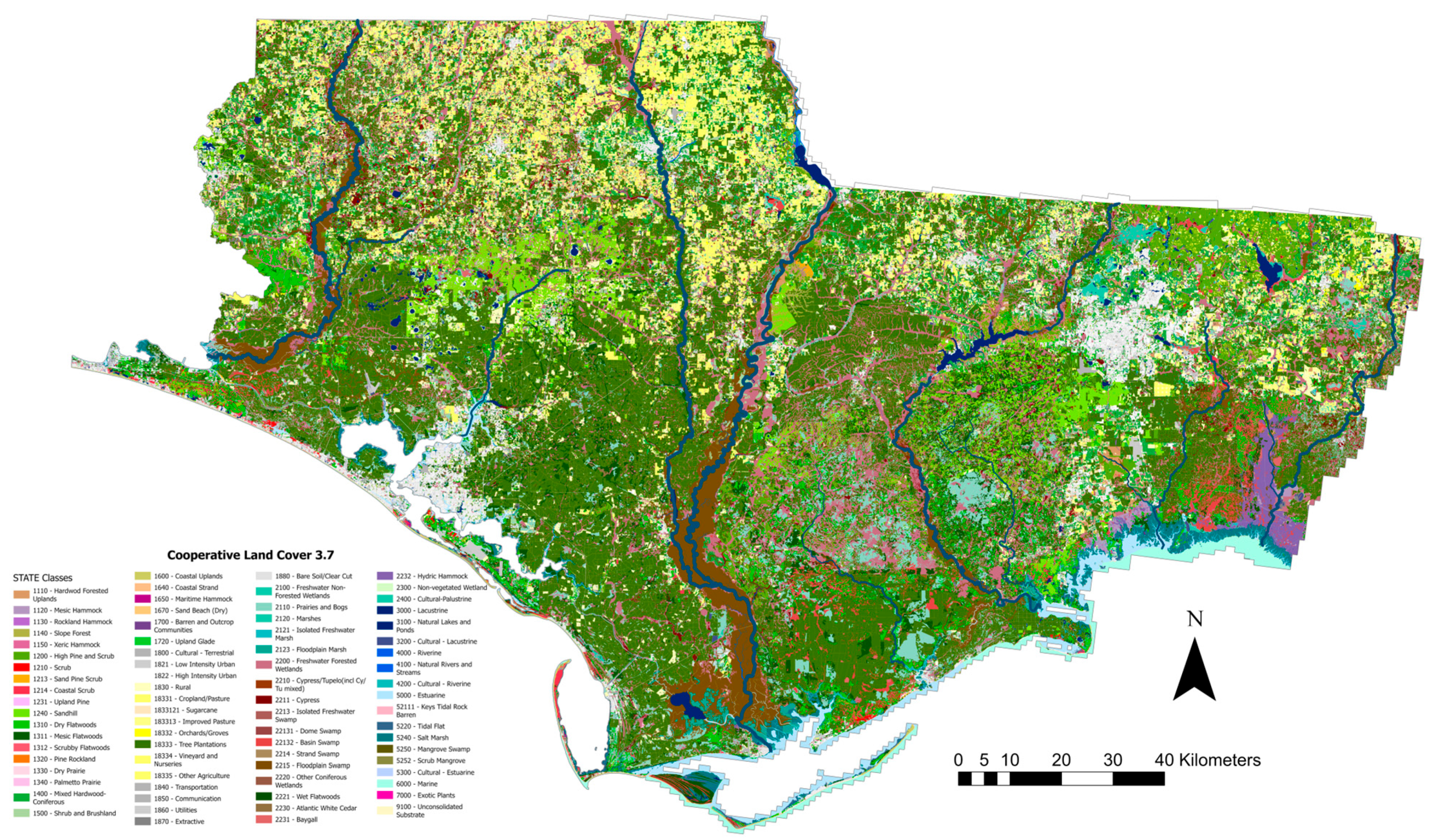
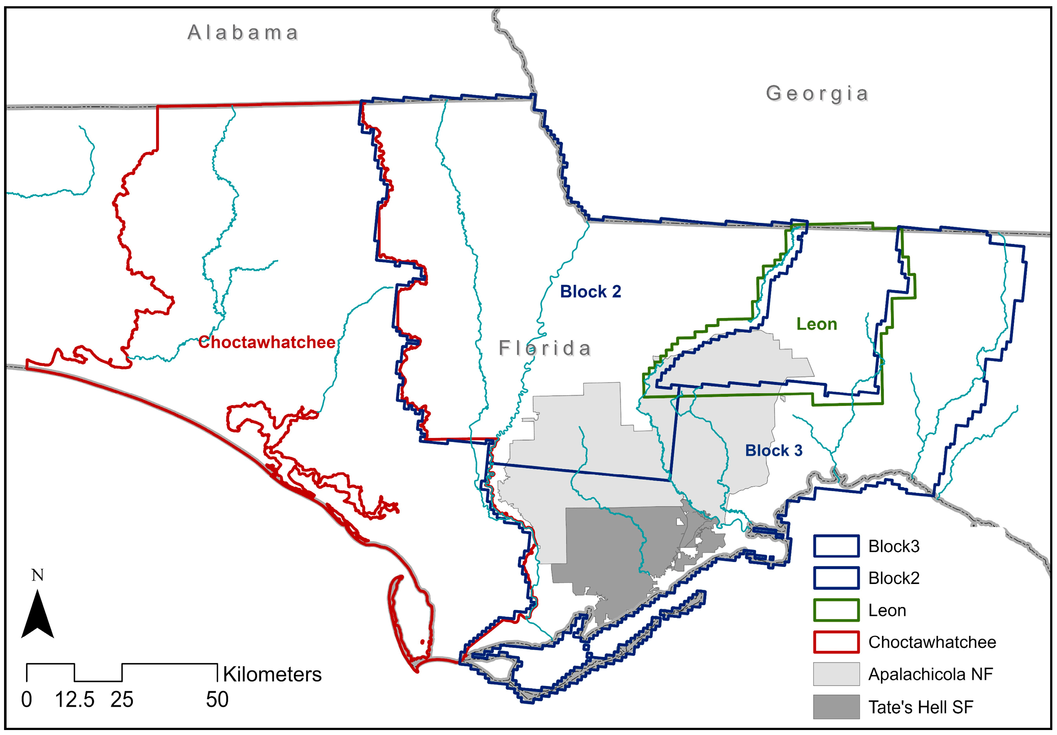
2.1. Study Area

The study area consisted of 11 counties in the panhandle of Florida, totaling roughly 22,900 km² (Figure 1). This area encompasses many federal, state, and private conservation lands, the largest of which are the Apalachicola National Forest and Tate’s Hell state forest. It is a well-known biodiversity hotspot in North America [26] and it is historically dominated by the critically endangered longleaf pine (Pinus palustris) forest ecosystem [27]. Several threatened and endangered plants and animals made their homes here, including the red-cockaded woodpecker (Leuconotopicus borealis), frosted flatwoods salamander (Ambystoma cingulatum), and Harper’s Beauty (Harperocallis flava) [28].

This area contains one major urban center, the city of Tallahassee, as well as several rivers, including the Choctawhatchee in the western side of the Choctawhatchee LiDAR block, the Apalachicola and Chipola rivers in the middle of our study area, forming the western border of the Apalachicola national forest, and the Ochlockonee river, which runs from the Georgia border around the western edge of Leon County and through the national forest. Forest is the dominant landcover type in this area. Specifically, according to the Cooperative Land Cover dataset [29], the major landcover types in this area are tree plantations, freshwater forested wetlands, mixed hardwood-coniferous, followed by prairies and bogs, cropland, and wet flatwoods. The full list of landcover types and the landcover map are shown in Appendix A.

2.2. LiDAR Datasets

The LiDAR data for this study were obtained and processed as four separate blocks of classified LAS version 1.4 files referred to as Block2, Block3, Choctawhatchee, and Leon. These data were downloaded from the United States Geological Survey 3D Elevation (3DEP) Program [30]. The Leon LiDAR block covered Leon County, Florida, and consisted of 876 LAS files covering 5000 ft2 of surface area with a nominal pulse spacing (NPS) of 0.35 m, approximately 8 pts/m². The Leon LiDAR block was acquired between 5 February 2018 and 25 April 2018 [31]. Block 2, Block 3 and Choctawhatchee consisted of 6845, 6598, and 3893 LAS files, respectively, of a size of 1 km² with an NPS of 0.7 m and approximately 2 pts/m². Block 2 and Block 3 LiDAR were collected in early 2018, while Choctawhatchee LiDAR data were acquired in early 2017 [32,33].

LiDAR Processing

LiDAR datasets were processed using the methods developed in [24], which used a custom R software v4.0.4 [34] script built within the lidR package [35,36]. The outputs were multiband raster datasets of relative height, density, and canopy cover at 5 m horizontal spatial resolution. This process resulted in twenty-four LiDAR metrics to be used as model predictor variables (

Table 1. LiDAR dataset raster bands, with raster band numbers and description.

Predictor Band	Description
1	Mean of all relative heights
2	Std. dev of all relative heights
3	Relative height 95%
4	Relative height 90%
5	Relative height 75%
6	Relative height 50%
7	Relative height 25%
8	Relative height 10%
9	Relative height 5%
10	Relative density 0.6096 m to 3.048 m (shrubs)
11	Relative density 3.048 m to 6.096 m (low midstory)
12	Relative density 6.096 m to 14.935 m (high midstory)
13	Relative density all returns ≥ 0.6096 m
14	Relative density all returns ≥ 3.048 m
15	Relative density all returns ≥ 6.096 m
16	Relative density all returns ≥ 14.935 m
17	Canopy cover ≥ 0.6096 m (based only on first returns)
18	Canopy cover ≥ 3.048 m (based only on first returns)
19	Canopy cover ≥ 6.096 m (based only on first returns)
20	Canopy cover ≥ 14.935 m (based only on first returns)
21	Mean of all relative heights ≥ 0.6096 m
22	Mean of all relative heights ≥ 3.048 m
23	Mean of all relative heights ≥ 6.096 m
24	Mean of all relative heights ≥ 14.935 m

). The mean and standard deviation of these twenty-four predictor bands were calculated for a 40 m × 40 m square moving window so that every 5 m pixel had values as if it were the center of a 40 m × 40 m square field plot.

2.3. Forest Plots

The 246 forested field plots used in this study were established between December 2017 and March 2018. These plots were designed as 36 m × 36 m square plots containing four 9 m radius non-overlapping subplots, following the recommendations of [25]. Plot design and locations were created to work with remotely sensed data, and the compact plot design was designed to maximize the observed area of a plot, while plot locations were selected to represent the range of remotely sensed data in the study area, specifically multispectral imagery from the Sentinel-2, Landsat and NAIP programs [25].

Subplot forest data consisted of the number and species of individual trees, tree condition, and diameter at breast height (DBH). Trees with DBH < 5 cm were counted but did not have their DBH individually measured. Additionally, vegetation cover, ground cover, coarse woody debris cover, and years since last burn for the subplot were also estimated.

Processing Forest Plot Data

Forest plot data were organized hierarchically in a Microsoft Access database by plot, subplot and individual trees. Pine trees species, defined as any tree species of the genus Pinus, were separated from all other tree species. Then, the trees were grouped by size, DBH < 25.4 cm, DBH 25.4 cm–35.6 cm, DBH > 35.6 cm of “pine”, “other” and “all” tree species, with the “all” category being the sum of “pine” and “other”. The BA per hectare values of these groups were summarized by plot. We chose the lower than 25.4 cm DBH group because of its relevance for forage analysis of red-cockaded woodpecker. The 35.6 cm DBH size trees are ideal for forage and nesting of red-cockaded woodpecker and can also be used as the minimum size for sawtimber [5]. In addition to the BA of each size category for the tree species groups, a presence or absence column for each of the tree size categories was calculated, with 1 indicating presence of that tree size within a plot and 0 indicating absence.

2.4. Basal Area Modeling by Tree Size

2.4.1. Single Model Selection

For our single-model approach, we initially tested the usefulness of using a presence and absence model to constrain our BA models to areas where the relevant DBH groups occurred, which had the advantage of eliminating zero inflating linear regression models. However, these presence models performed poorly. So, we moved on to model BA directly.

Multiple linear regression modeling was carried out in the R software environment [34]. The response variable for the regression models was the basal area for each of the DBH groups for both a ‘pine’ and ‘all’ tree group, resulting in 6 total multiple linear regression models. From the examination of the distribution of response variables, we determined that the use of an exponential model for the all-tree species basal area lower than 25.4 cm DBH class would be appropriate. The other five models used a linear distribution. The multiple linear regression models’ predictor variables were selected from the 48 LiDAR variables created from the mean and standard deviation of the variables of Table 1 following the methods described in [24].

The variable selection process for our linear models used a sequential forward stepwise general additive model (GAM) routine that followed the R script [37]. For these models, we chose to use the Gaussian family and identity link distribution, an alpha of 1, and an increase in percent deviance threshold of 0.005 to make the selection more inclusive. After the initial variable selection using the forward stepwise process, we created a linear model with the selected response variables. This initial model had an abundance of predictor variables that were then iteratively removed based on their level of significance. This process continued by removing the least significant predictor variables and then recreating a multiple linear model to assess the significance of the remaining predictor variables. When only significant predictor variables remained with p-values lower than 0.05, the model was considered complete.

The 6 resulting multiple regression models were applied to our spatial variables to create the resulting raster surfaces of basal area by DBH size class and tree group, which was carried out using the ‘create raster from model’ tool in the RMRS Raster Utility ArcMap plug-in [38]. An additional regional predictor variable was added to the three pine tree models to address the disparity in LiDAR sensor and point density between the Leon block and the other three LiDAR blocks. This regional variable was a simple 1 value for all Leon plots and a 0 value for all other plots. The six DBH class models are shown below.

All Tree BA < 25.4 cm = −0.2043745 + 0.4429096 × Band1 + 0.3827406 × Band2 − 0.4009239 × Band5 − 0.1892984 × Band6 + 1.6947138 × Band17 + 4.7259355 × Band18,

(1)

All Tree BA 25.4 cm to 35.6 cm = 0.03977877 + 26.41526333 × Band15 + 53.71854445 × Band20 − 6.04134412 × SD of Band1 − 5.83702227 × SD of Band9 + 108.65857472 × SD of Band11

(2)

All Tree BA > 35.6 cm = −2.851847 + 28.677864 × Band1 − 7.434963 × Band5 + 466.253215 × Band11 + 331.142580 × Band12 − 54.710936 × Band13 − 449.124076 × Band14 + 175.396993 × Band20 + 5.415879 × SD of Band1

(3)

Pine Tree BA < 25.4 cm = 0.9332988 − 9.3001079 × Band1 + 13.9685948 × Band7 − 24.0162990 × Band8 + 21.7309721 × Band9 − 152.7182669 × Band10 + 125.6686470 × Band17 − 1.4066225 × Leon_y_n

(4)

Pine Tree BA 25.4 cm to 35.6 cm = −0.5551019 + 4.3163379 × Band7 + 8.0742821 × Band17 − 3.3014085 × SD of Band2 − 6.4555188 × SD of Band9 + 1.3641338 × SD of Band21 + 6.4696840 × Leon_y_n

(5)

Pine Tree BA > 35.6 cm = −1.916267 + 9.031668 × Band7 + 6.023839 × SD of Band7 − 26.276214 × SD of Band8 + 19.654782 × SD of Band9 + 13.719508 × Leon_y_n

(6)

where ‘Band#’ refers to the LiDAR dataset output bands of Table 1 and was calculated as the mean value of a 40 m × 40 m plot. ‘SD of Band#’ refers to the standard deviation of a 40 m × 40 m plot of the LiDAR dataset output band of Table 1. ‘Leon_y_n’ refers to the regional variable.

2.4.2. Ensemble Linear Model

In addition to the linear models of our six response variables, we also created ensemble linear models (ELMs). The methodology used to create ELMs was adapted from the methods of [25], using linear models in place of GAMs. Within the R software, this was achieved by substituting the lm() function for the gam() function. The full R script is detailed in Appendix B.

The ELMs were informed with the same predictor variables that were used in the single models. The major difference between these methods was that the ensemble models only used a portion of the training data (i.e., the forest plots) to train a linear model. This approach was repeated 50 times, using random sampling with replacement to select 75% of the training data for each model iteration. Each of these 50 linear models generated an output and the mean of these values was used as the estimate of the response variable. Additionally, standard error results were produced spatially using the variability in the 50 ensemble models outputs at each raster cell.

2.4.3. Ensemble Generalized Additive Model

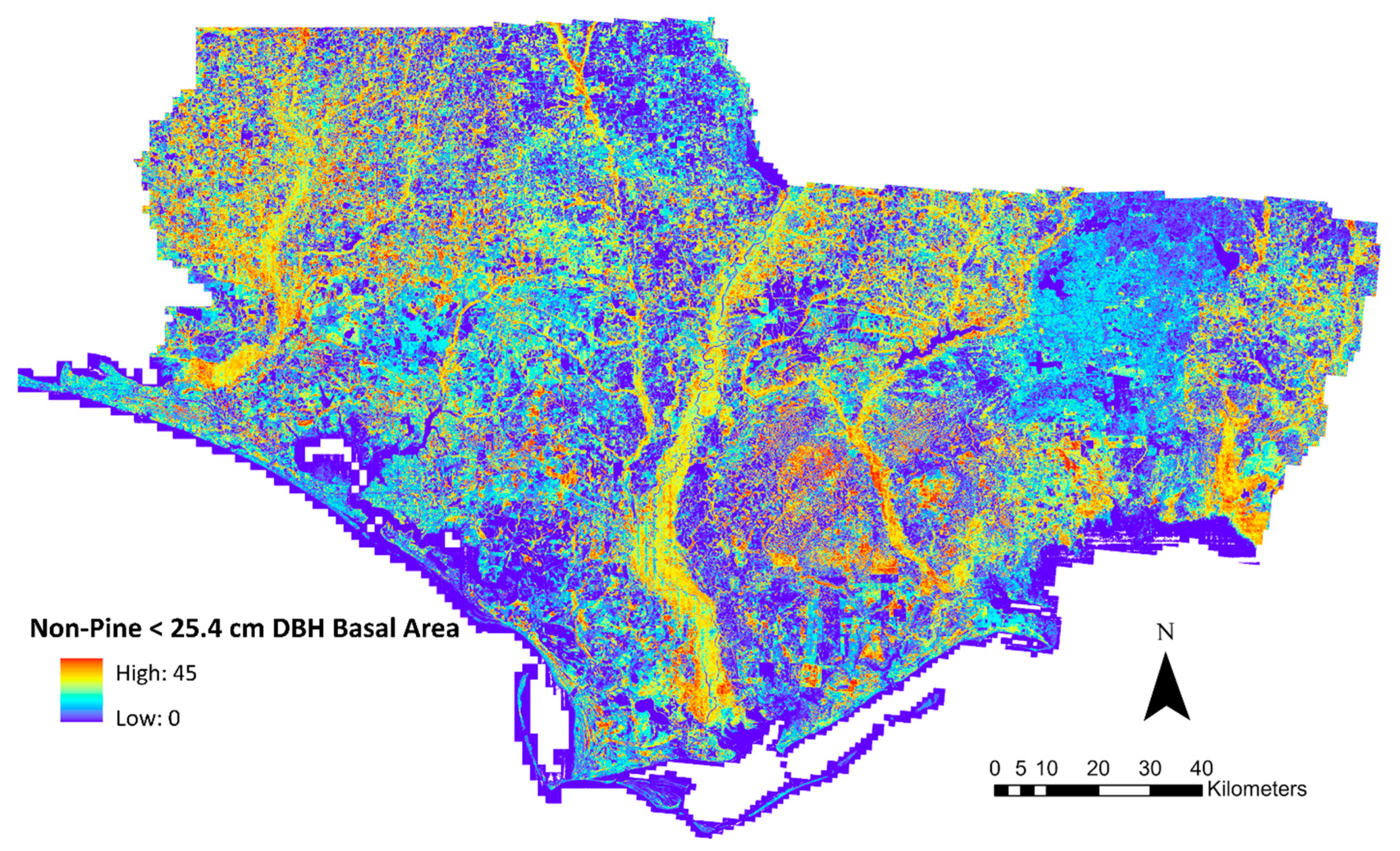
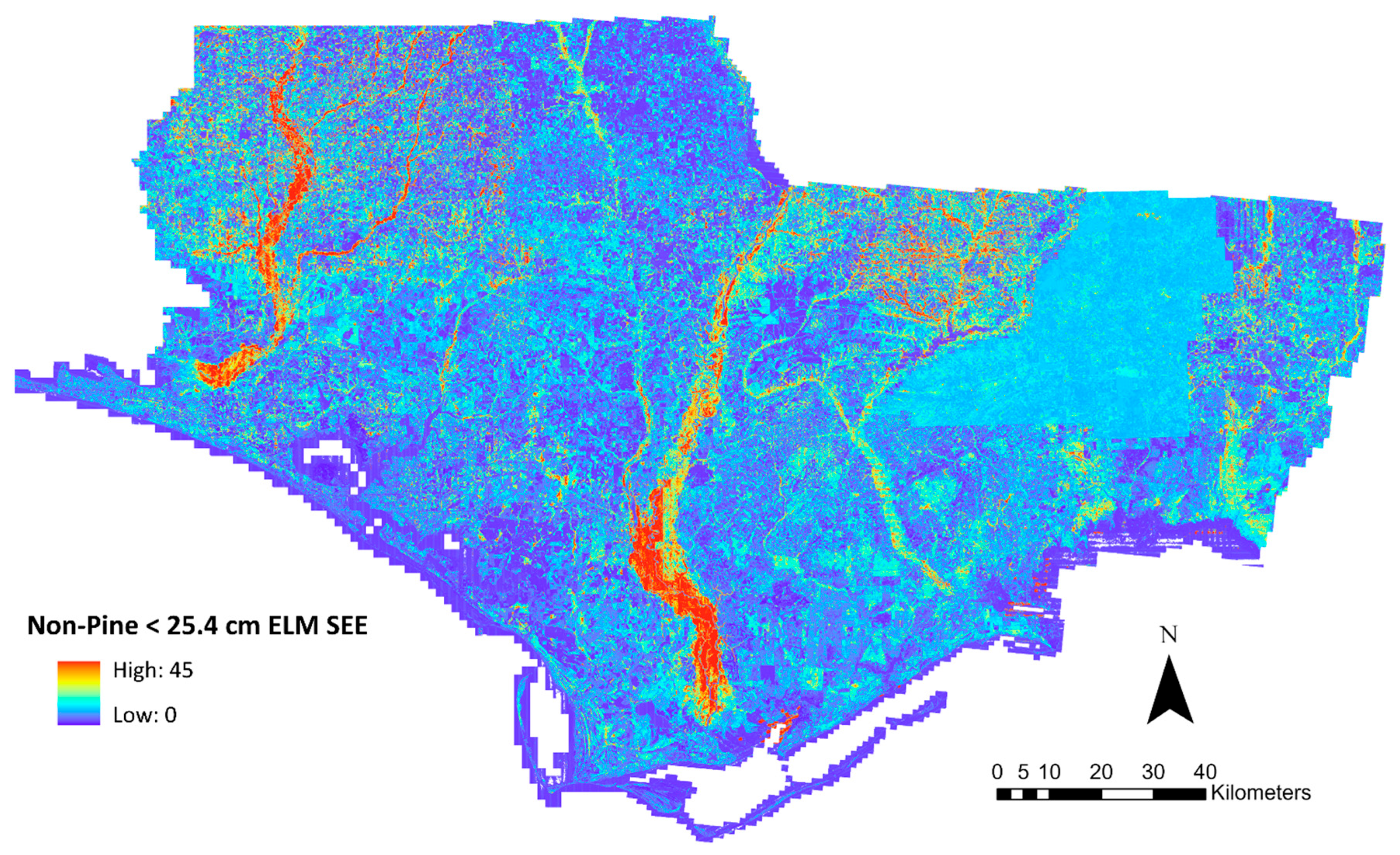
Our third modeling approach used ensemble generalized additive modeling (EGAM) to estimate 6 response variables. This method followed those of [25], with one major change being the use of the predictor variables selected from the single-model approach step to inform the models as opposed to running a predictor variable selection process specifically for the EGAMs. A step-by-step tutorial on this methodology is available online [39].

The EGAMs used the same parameters as the ELMs, except for the three pine models where the regional effect was not considered. Their removal was necessary because the regional effect had only two values, which was insufficient for setting up a basis function in a GAM. The EGAM was similarly trained by 75% of the input data at a time, and 50 models were created for each response variable. The EGAM method also produced a mean value raster and a standard error value raster.

2.5. Raster Outputs

Single-model raster outputs were created using the “create raster from model” tool in the RMRS Raster Utility ArcMap toolbar [38], which used the model file and the raster surfaces of the predictor variables to each cell of the predictor raster. The output of this tool was a raster of predicted BA values within the specified DBH class. The final processing steps on the raster outputs consisted of setting the negative values of this tool’s raster output to zero and setting the values outside the observed range of BA for each DBH class to a “no data value” using the “remap values” tool in the RMRS Raster Utility Toolbar. The single-model raster outputs were then converted to unsigned 16-bit files, which rounded the values to the nearest integer, before combining into a single raster covering the study area using the “Mosaic raster” function in ArcMap. The order of overlap for this mosaic was Block2, Block3, Choctawhatchee, and finally Leon. The exponential models used for the “All” tree species with a DBH lower than 25.4 cm had an extra step of post processing where the values were transformed from their log values using the “exponential math transformation” tool in the RMRS Raster Utility toolbar.

Both ensemble model workflows produced two raster outputs within R, the mean cell value, and standard error raster. These raster outputs were saved with negative values set to zero, which were combined into mosaic datasets following the same process as our single-model outputs.

3. Results

The summary statistics for our model results showed that the EGAMs had the highest r-squared values and the lowest RMSE values for all three DBH size classes for both pine and all tree species groups (

Table 2. Summary results for models of basal area per hectare by tree DBH class. RMSE unit is meters squared per hectare. The best values for each tree DBH class are in bold. The “All” tree species with DBH < 25.4 cm was an exponential model, while all other models used a linear model. The pine models included a regional effect for the Leon block, except for the EGAMs.

All Tree Species	r2	RMSE	Pine Tree Species	r2	RMSE
DBH < 25.4 Single Model	0.657	6.52	DBH < 25.4 Single Model	0.657	5.25
DBH < 25.4 ELM	0.516	8.27	DBH < 25.4 ELM	0.667	5.12
DBH < 25.4 EGAM	0.675	6.51	DBH < 25.4 EGAM	0.731	4.61
DBH 25.4–35.56 Single Model	0.447	4.01	DBH 25.4–35.56 Single Model	0.445	3.29
DBH 25.4–35.56 ELM	0.456	3.93	DBH 25.4–35.56 ELM	0.459	3.20
DBH 25.4–35.56 EGAM	0.514	3.72	DBH 25.4–35.56 EGAM	0.511	3.04
DBH > 35.56 Single Model	0.709	4.37	DBH > 35.56 Single Model	0.593	4.37
DBH > 35.56 ELM	0.712	4.35	DBH > 35.56 ELM	0.606	4.26
DBH > 35.56 EGAM	0.805	3.59	DBH > 35.56 EGAM	0.623	4.16

). The ELMs had better r-squared and RMSE values than the single model for all models except the “All” tree species with a DBH lower than 25.4 cm model.

We measured the production time from the final model to raster outputs for the three modeling methods. The single model approach was practically instantaneous using the RMRS Raster Utility’s “create raster from model” tool [38]. The only notable processing time was the amount of time it took to save the raster to disk, which was equivalent for all three approaches and ignored for comparison purposes. The ensemble models’ processing time was more substantial. The ELMs took anywhere from 7 min to process the smaller Leon block to 33 ½ min for the large Choctawhatchee block. The EGAMs took 25–33 times longer to process than the ensemble linear models (

Table 3. Processing time in minutes for each LiDAR block by model for ensemble linear model (ELM) and ensemble general additive model (EGAM) of the pine tree workflows. The rounded difference between the modeling times is shown in the final column. >25.4 refers to modeling basal area of trees lower than 25.4 cm DBH, 25.4–35.56 refers to modeling basal area of trees between 25.4 cm and 35.56 cm DBH, and <35.56 refers to modeling basal area of trees greater than 35.56 cm DBH.

LiDAR Block and Model	ELM	EGAM	Difference in Multiples
Block3 Pine < 25.4	21.8	656.6	30
Block3 Pine 25.4–35.56	19.2	538.1	28
Block3 Pine > 35.56	17.4	456.0	26
Block2 Pine < 25.4	24.3	791.6	33
Block2 Pine 25.4–35.56	17.5	606.0	35
Block2 Pine > 35.56	17.6	535.9	30
Chocta Pine < 25.4	33.5	991.7	30
Chocta Pine 25.4–35.56	30.4	752.0	25
Chocta Pine > 35.56	23.8	663.0	28
Leon Pine < 25.4	6.9	229.0	33
Leon Pine 25.4–35.56	7.3	192.3	26
Leon Pine > 35.56	6.8	172.5	25

). To isolate the effect of model type on processing time, both the ELM and EGAM workflows used the same number of logical cores on the same laptop with the same input variable rasters (see Appendix A).

Single-model raster outputs consisted of the estimated value of BA for each DBH size class and tree type (Figure 2). The ELMs and EGAMs estimated BA as the mean value from the 50 ensemble models and produced a spatially explicit standard error estimate (Figure 3). This standard error raster can be used to identify areas of high variability in the model estimates. In this project, a total of sixty individual rasters of BA and standard error estimates were created.

When compared to the other three LiDAR blocks, the effect of higher LiDAR resolution in the Leon block was visually apparent in all non-pine models (Figure 2 and Figure 3), and only faintly visible in the all-tree models (Figure 4). While adding a regional effect somewhat mitigated the above effect in the non-pine single models, both ensemble models showed distinct differences in the Leon block raster outputs compared to the other three blocks. This difference appeared regardless of whether the regional effect was included in the predictor variables, as was the case with the ensemble linear models, or was excluded, as was the case with the EGAMs.

The three classes of estimates of BA by DBH class were summed to provide an estimate of overall tree BA for both the “All” and “Pine” tree groups. These results were compared to those of our previous studies that used a single-model approach to estimate total BA in the same study area (

Table 4. The r-squared and root mean square error of the summed BA of our three DBH size classes, by tree grouping and model approach. Our previous study’s total estimated tree BA summary statistics are provided for comparison.

Model	r2	RMSE
All Single Model	0.726	9.84
All ELM	0.724	9.86
All EGAM	0.791	8.63
Pine Single Model	0.740	8.43
Pine ELM	0.742	8.40
Pine EGAM	0.773	7.87
St. Peter, et al., 2021 [24]	r2	RMSE
All Model	0.777	7.67
Pine Model	0.687	5.62

). The three approaches used in this study had similar or higher r-squared values, but worse RMSE values, compared to the direct estimates of total BA found in our previous study [24].

4. Discussion

The results of this study demonstrated the accuracy and efficiency of estimating the BA of tree diameter classes directly as opposed to modeling a diameter distribution and then deriving various forest metrics from a modeled distribution. Directly estimating the BA reduced the complexity of the modeling effort and allowed for an easier entry point for non-statisticians. The DBH class breaks were chosen to be immediately relevant to wildlife managers and for timber planning without the need to summarize multiple smaller classes. Additionally, estimating three larger classes instead of the entire tree stem distribution avoided making assumptions about the shape of the distribution, which can be highly variable in a large and diverse forest landscape like the one used in this study. Area-based methods that relied on Weibull or other distributions had the spatial horizontal resolution of a plot, while our method maintained the native spatial resolution of the LiDAR metrics (5 m² in this study). It is possible to create these continuous raster outputs using area-based methods that fit a Weibull function to each plot; however, doing it in a continuous manner across a large landscape would require immense processing power [9].

In addition, the classes selected in this study were non-overlapping and comprehensive, allowing them to be summed in part to create other class divisions, such as all trees with a DBH lower than 35.56 cm or create an estimate of total BA for all DBH classes. However, based on our comparison to a previous model of total BA (Table 4), we would recommend modeling total BA directly.

LiDAR data had previously been used to directly build regression models that estimated the BA of different DBH classes of trees for wildlife habitat. Garabedian et al., 2014 [7] estimated pine BAs for trees with a DBH greater than 25.4 cm and greater than 35.56 cm, as well as for hardwood trees with a DBH greater than 22.86 cm (9″), and used them in their analysis of forage habitat for red-cockaded woodpecker in their South Carolina study area [7]. Our results, as shown in Table 2, compared well with those of a previous study [7] that used a LiDAR dataset with a point density of 10 points/m² to inform multiple linear regression models of BA of pine trees above 25.4 cm and a DBH above 35.56 cm, with r-squared values of 0.74 and 0.80, respectively, and RMSE of 22.5 and 16.9. These results were comparable to those of our EGAMs of “All” tree species with a DBH greater than 35.56 cm with an r-squared value of 0.805 and an RMSE of 15.63, using a LiDAR dataset with a lower overall point density (2 and 8 points/m²). Spriggs et al., 2017 [8] used LiDAR with a moderate point density of 2 points/m², equivalent to the point density of three of the LiDAR collections used in this study, to predict the SDD and then calculate basal area with an RMSE of 6.99 m²/ha for all tree species (5.93 m²/ha for broadleaf, and 7.39 m²/ha for conifer). All the models produced in this study, except the small tree models (DBH < 25.4), had lower RMSE values, as shown in Table 2.

The higher-point-density LiDAR dataset in the Leon block (8 points/m²) led to visually apparent differences in the estimation of that block when compared to the other three blocks, especially in the pine tree models. This is a known issue when using LiDAR datasets with different acquisition properties [9,40,41,42]. We recommend that future forest structure models avoid combining LiDAR datasets with significantly different resolutions if possible. Additional analysis on how this data heterogeneity affects model results is needed.

The three modeling methods compared here had different strengths and weaknesses. The single-model approach gave good estimates, was the simplest to interpret, and is likely to be familiar to most practitioners. The ensemble method provided more accurate estimates with additional raster of spatially explicit standard error estimates. The ELM approach had the easy interpretability of a linear model, though there were more linear models to interpret (fifty, in this case). The ELM was also produced on average 30 times faster than the EGAM rasters. The EGAMs had the highest r-squared values and the lowest RMSE of the approaches but were harder to interpret while also taking much longer to produce than any of the other approaches. Though the specific predictor variables selected for models and accuracies of the modeled results will vary in other landscapes, the comparisons we highlight here are due to the nature of the different modeling approaches. Therefore, we believe that these results are relevant in forest types outside of our study area.

The interpretation of GAMs relied on the understanding of the smoothing function applied to each predictor variable, which often required visual inspection of plots for each term and interpretation of the interaction effects, making GAMs more complex than linear models whose predictor variables’ effect can often be summarized in a single number. This complexity was exacerbated when outputs were a result of an ensemble of 50 GAMs.

The results of this study showed that modeling BA directly for select tree DBH size classes created outputs as good or better than those of previously published methods. We also demonstrated the advantages and limitations that ensemble models can provide. The benefits and drawbacks of these three approaches can help forest managers make informed decisions on which approach best fits their needs when they decide to produce similar outputs for their own forested landscapes.

References

1. Coomes, D.A.; Allen, R.B. Effects of size, competition and altitude on tree growth. J. Ecol. 2007, 95, 1084–1097. [Google Scholar] [CrossRef]
2. Konôpka, B.; Pajtík, J.; Moravčík, M.; Lukac, M. Biomass partitioning and growth efficiency in four naturally regenerated forest tree species. Basic Appl. Ecol. 2010, 11, 234–243. [Google Scholar] [CrossRef]
3. Duchateau, E.; Schneider, R.; Tremblay, S.; Dupont-Leduc, L. Density and diameter distributions of saplings in naturally regenerated and planted coniferous stands in Québec after various approaches of commercial thinning. Ann. For. Sci. 2020, 77, 38. [Google Scholar] [CrossRef]
4. Leclère, L.; Lejeune, P.; Bolyn, C.; Latte, N. Estimating Species-Specific Stem Size Distributions of Uneven-Aged Mixed Deciduous Forests Using ALS Data and Neural Networks. Remote Sens. 2022, 14, 1362. [Google Scholar] [CrossRef]
5. Nordman, C.; White, R.; Wilson, R.; Ware, C.; Rideout, C.; Pyne, M.; Hunter, C. Rapid Assessment Metrics to Enhance Wildlife Habitat and Biodiversity Within Southern Open Pine Ecosystems; U.S. Fish and Wildlife Service and NatureServe, for the Gulf Coastal Plains and Ozarks Landscape Conservation Cooperative: Tallahassee, FL, USA, 2016; Available online: https://www.natureserve.org/sites/default/files/openpinemetrics-finalreport_12may16.pdf (accessed on 4 November 2024).
6. America’s Longleaf. 2014 Longleaf Pine Maintenance Condition Class Definitions. Available online: https://americaslongleaf.org/media/mjroaokz/final-lpc-maintenance-condition-class-metrics-oct-2014-high-res.pdf (accessed on 4 November 2024).
7. Garabedian, J.E.; McGaughey, R.J.; Reutebuch, S.E.; Parresol, B.R.; Kilgo, J.C.; Moorman, C.E.; Peterson, M.N. Quantitative analysis of woodpecker habitat using high-resolution airborne LiDAR estimates of forest structure and composition. Remote Sens. Environ. 2014, 145, 68–80. [Google Scholar] [CrossRef]
8. Gove, J.H.; Patil, G.P. Modeling the Basa Area-size Distribution of Forest Stands: A Compatible Approach. For. Sci. 1999, 44, 285–297. [Google Scholar]
9. Spriggs, R.A.; Coomes, D.A.; Jones, T.A.; Caspersen, J.P.; Vanderwel, M.C. An Alternative Approach to Using LiDAR Remote Sensing Data to Predict Stem Diameter Distributions across a Temperate Forest Landscape. Remote Sens. 2017, 9, 944. [Google Scholar] [CrossRef]
10. Coomes, D.A.; Dalponte, M.; Jucker, T.; Asner, G.P.; Banin, L.F.; Burslem, D.; Simon, L.L.; Nilus, R.; Phillips, O.L.; Phua, M.; et al. Area-based vs tree-centric approaches to mapping forest carbon in Southeast Asian forests from airborne laser scanning data. Remote Sens. Environ. 2017, 194, 77–88. [Google Scholar] [CrossRef]
11. Fu, L.; Duan, G.; Ye, Q.; Meng, X.; Luo, P.; Sharma, R.P.; Sun, H.; Wand, G.; Liu, Q. Prediction of Individual Tree Diameter Using a Nonlinear Mixed-Effects Modeling Approach and Airborne LiDAR Data. Remote Sens. 2020, 12, 1066. [Google Scholar] [CrossRef]
12. Maltamo, M.; Gobakken, T. Predicting Tree Diameter Distributions. In Forestry Applications of Airborne Laser Scanning: Concepts and Case Studies; Maltamo, M., Næsset, E., Vauhkonen, J., Eds.; Springer Science+Business Media: Dordrecht, The Netherlands, 2014; pp. 177–193. [Google Scholar] [CrossRef]
13. Persson, Å.; Holmgren, J.; Söderman, U. Detecting and measuring individual trees using an airborne laser scanner. Photogramm. Eng. Remote Sens. 2002, 68, 357–363. [Google Scholar]
14. Vauhkonen, J.; Ene, L.; Gupta, S.; Heinzel, J.; Holmgren, J.; Pitkänen, J.; Solberg, S.; Wang, Y.; Weinacker, H.; Hauglin, K.M.; et al. Comparative testing of single-tree detection algorithms under different types of forest. For. Int. J. For. Res. 2012, 85, 27–40. [Google Scholar] [CrossRef]
15. Gobakken, T.; Næsset, E. Estimation of Diameter and Basal Area Distributions in Coniferous Forest by Means of Airborne Laser Scanner Data. Scand. J. For. Res. 2004, 19, 529–542. [Google Scholar] [CrossRef]
16. Zhang, Z.; Wang, T.; Skidmore, A.K.; Cao, F.; She, G. An improved areas-based approach for estimating plot-level tree DBH from airborne LiDAR data. For. Ecosyst. 2023, 10, 100089. [Google Scholar] [CrossRef]
17. Breidenbach, J.; Gläser, C.; Schmidt, M. Estimation of diameter distributions by means of airborne laser scanner data. Can. J. For. Res. 2008, 38, 1611–1620. [Google Scholar] [CrossRef]
18. Bollandsås, O.M.; Maltamo, M.; Gobakken, T.; Næsset, E. Comparing parametric and non-parametric modelling of diameter distributions on independent data using airborne laser scanning in a boreal conifer forest. Forestry 2013, 86, 493–501. [Google Scholar] [CrossRef]
19. Mauro, F.; Frank, B.; Monleon, V.J.; Temesgen, H.; Ford, K.R. Prediction of diameter distributions and tree-lists in southwestern Oregon using LiDAR and stand-level auxiliary information. Can. J. For. Res. 2019, 49, 775–787. [Google Scholar] [CrossRef]
20. Packalén, P.; Maltamo, M. Estimation of species-specific diameter distributions using airborne laser scanning and aerial photographs. Can. J. For. Res. 2008, 38, 1750–1760. [Google Scholar] [CrossRef]
21. Maltamo, M.; Eerikäinen, K.; Pitkänen, J.; Hyyppä, J.; Vehmas, M. Estimation of timber volume and stem density based on scanning laser altimetry and expected tree size distribution functions. Remote Sens. Environ. 2004, 90, 319–330. [Google Scholar] [CrossRef]
22. Trager, M.D.; Drake, J.B.; Jenkins, A.M.; Petrick, C.J. Mapping and Modeling Ecological Conditions of Longleaf Pine Habitats in the Apalachicola National Forest. For. Ecol. 2018, 116, 304–311. [Google Scholar] [CrossRef]
23. Meijer, C.; Grootes, M.; Koma, Z.; Dzigan, Y.; Gonçalves, R.; Andela, B.; van den Oord, G.; Ranguelova, E.; Renaud, N.; Kissling, W. Laserchicken—A tool for distributed feature calculation from massive LiDAR point cloud datasets. SoftwareX 2020, 12, 100626. [Google Scholar] [CrossRef]
24. St. Peter, J.; Drake, J.; Medley, P.; Ibeanusi, V. Forest Structural Estimates Derived Using a Practical, Open-Source Lidar-Processing Workflow. Remote Sens. 2021, 13, 4763. [Google Scholar] [CrossRef]
25. Hogland, J.; Affleck, D.L.; Anderson, N.; Seielstad, C.; Dobrowski, S.; Graham, J.; Smith, R. Estimating Forest Characteristics for Longleaf Pine. Forests 2020, 11, 426. [Google Scholar] [CrossRef]
26. Stein, B.A.; Kutner, L.S.; Adams, J.S. Precious Heritage: The Status of Biodiversity in the United States; Oxford University Press: New York, NY, USA, 2000. [Google Scholar]
27. Noss, R.F. The longleaf pine landscape of the Southeast: Almost gone and almost forgotten. Endanger. Species Update 1988, 5, 1–8. [Google Scholar]
28. Oswalt, C.; Cooper, J.; Brockway, D.; Brooks, H.; Walker, J.; Connor, K.; Oswalt, S.N.; Conner, R.C. History and Current Condition of Longleaf Pine in the Southern United States; U.S. Department of Agriculture Forest Service, Southern Research Station: Ashville, NC, USA, 2012. [Google Scholar]
29. Cooperative Land Cover, Version 3.7. Published November 2023. Available online: https://myfwc.com/research/gis/wildlife/cooperative-land-cover/ (accessed on 18 December 2024).
30. United States Geological Survey. 3D Elevation Program. USGS Core Science Systems. Available online: https://www.usgs.gov/core-science-systems/ngp/3dep/what-is-3dep?qt-science_support_page_related_con=0#qt-science_support_page_related_con (accessed on 2 August 2021).
31. NOAA Fisheries. OCM Partners 2018 TLCGIS Lidar: Leon County, FL. Available online: https://www.fisheries.noaa.gov/inport/item/60045 (accessed on 25 June 2021).
32. NOAA Fisheries. OCM Partners 2018 USGS Lidar: Florida Panhandle. Available online: https://www.fisheries.noaa.gov/inport/item/58298 (accessed on 25 June 2021).
33. NOAA Fisheries. OCM Partners 2017 NWFWMD Lidar: Lower Choctawhatchee. Available online: https://www.fisheries.noaa.gov/inport/item/55725 (accessed on 25 June 2021).
34. R Core Team. R. A Language and Environment for Statistical Computing. In R Foundation for Statistical Computing; R Core Team: Vienna, Austria, 2021; Available online: https://www.R-project.org/ (accessed on 25 October 2024).
35. Roussel, J.; Auty, D.; Coops, N.; Tompalski, P.; Goodbody, T.; Meador, A.; Bourdon, J.; de Boissieu, F.; Achim, A. lidR: An R package for analysis of Airborne Laser Scanning (ALS) data. Remote Sens. Environ. 2020, 251, 112061. [Google Scholar] [CrossRef]
36. Roussel, J.; Auty, D. Airborne LiDAR Data Manipulation and Visualization for Forestry Applications. R Package Version 3.1.4. Available online: https://cran.r-project.org/package=lidR (accessed on 4 November 2024).
37. Hogland, J.; Anderson, N.; Affleck, D.L.; St. Peter, J. Using Forest Inventory Data with Landsat 8 Imagery to Map Longleaf Pine Forest Characteristics in Georgia, USA. Remote Sens. 2019, 11, 1803. [Google Scholar] [CrossRef]
38. Hogland, J. Rocky Mountain Research Station, RMRS Raster Utility. Available online: https://research.fs.usda.gov/rmrs/products/dataandtools/tools/rmrs-raster-utility (accessed on 4 November 2024).
39. Hogland, J. Ensemble Generalized Additive Models (EGAM). Jupyter Notebook. Available online: https://colab.research.google.com/drive/1GnRagruTUCoPJQZSkZ2vMKS9aAKgnhEw?usp=sharing (accessed on 4 November 2024).
40. Asner, G.; Mascaro, J. Mapping tropical forest carbon: Calibrating plot estimates to a simple LiDAR metric. Remote Sens. Environ. 2014, 140, 614–624. [Google Scholar] [CrossRef]
41. Næsset, E. Effects of different flying altitudes on biophysical stand properties estimated from canopy height and density measured with small-footprint airborne scanning laser. Remote Sens. Environ. 2004, 91, 243–255. [Google Scholar] [CrossRef]
42. LaRue, E.A.; Fahey, R.; Fuson, T.L.; Foster, J.R.; Matthes, J.H.; Krause, K.; Hardiman, B.S. Evaluating the sensitivity of forest structural diversity characterization to LiDAR point density. Ecosphere 2022, 13, e4209. [Google Scholar] [CrossRef]
Figure 1. Study area in the Florida panhandle (~22,900 km2). The area of each LiDAR dataset is shown in different colors. Block2 and Block3 are shown using the same color as these datasets were collected at the same time and separated during post processing. The Apalachicola National Forest and Tate’s Hell state forest are shown in gray.
Remotesensing 17 00253 g001
Figure 2. Non-pine BA m2/ha of trees < 25.4 cm DBH using the single-model raster output. Note the Leon block with clearly visible value differences.
Remotesensing 17 00253 g002
Figure 3. ELM standard error estimate output in m2/ha for pine BA < 25.4 cm DBH.
Remotesensing 17 00253 g003
Figure 4. All tree species BA in m2/ha of trees < 25.4 cm diameter at breast height using the single-model raster output.
Remotesensing 17 00253 g004