Derivation of Hyperspectral Profiles for Global Extended Pseudo Invariant Calibration Sites (EPICS) and Their Application in Satellite Sensor Cross-Calibration

Abstract

This study presents the selection of 20 Extended Pseudo Invariant Calibration Sites (EPICS) for radiometric calibration and the derivation of their hyperspectral profiles using the DLR Earth Sensing Imaging Spectrometer (DESIS) and Hyperion data. The hyperspectral profile of one of these clusters, the GONA-EPICS cluster, was validated against ground truth measurements from the RadCalNet Gobabeb Namibia (GONA) site, demonstrating statistical agreement within their respective uncertainties through Welch’s test. The applicability of these hyperspectral profiles was further evaluated by generating Spectral Band Adjustment Factor (SBAF) between Landsat 8 and Sentinel-2A using the GONA-EPICS hyperspectral profile and comparing them to SBAF values derived from RadCalNet GONA site measurements. SBAF results were statistically the same, while SBAF derived from the combined DESIS and Hyperion data exhibited reduced uncertainty compared to those derived using Hyperion data alone, which is attributed to DESIS’s finer spectral resolution (2.5 nm vs. 10 nm). To assess EPICS applicability in cross-calibration, Cluster 13-GTS, which includes pixels from the Libya 4 CNES ROI, was used as a target. Cross-calibration gains obtained using EPICS and the T2T cross-calibration methodology were compared to those from the traditional cross-calibration approach using Libya 4 CNES ROI. Results demonstrated statistically similar gains, with EPICS achieving an uncertainty better than 6% across all bands compared to 4.4% for the traditional method, while enabling global coverage for daily cross-calibration opportunities. This study introduces globally distributed EPICS with validated hyperspectral profiles, offering enhanced spectral resolution and reliability for radiometric calibration and stability monitoring. The methodology supports efficient global scale sensor calibration and prepares for future hyperspectral missions.

1. Introduction

Over the past 40 years, a substantial number of Earth observation satellites were launched, providing data for various scientific applications such as vegetation monitoring, urban development tracking, and climate change studies [1,2,3,4]. The outcomes of these applications are crucial for understanding the Earth’s surface and its changes. To ensure data quality, the sensors on these satellites undergo pre-launch radiometric calibration. However, these sensors may degrade over time, needing routine stability monitoring and post-launch radiometric calibration [5].

Post-launch radiometric calibration can be achieved using onboard calibration systems. However, not all satellite sensors are equipped with these systems due to their high cost and potential degradation over time. Alternative techniques for radiometric calibration include vicarious calibration that evaluates radiance and irradiance, or reflectance-based approaches requiring in situ measurements. This method can be costly and time-consuming [6,7,8].

Cross-calibration offers an alternative to onboard calibration systems and vicarious calibration requiring field measurements. This technique involves transferring radiometric calibration from a well-calibrated sensor to an uncalibrated one, aligning both sensors to a common radiometric scale. It addresses the limitations of vicarious calibration, which often involves costly field measurements and personnel, as well as onboard calibrators, which can degrade over time and may not be present on all satellites [9,10,11].

Effective cross-calibration relies on using stable ground targets. Ideally, observations from both sensors should be collected over the same location at the same time with identical viewing and solar geometries. However, such ideal conditions are infrequent. Therefore, cross-calibration often employs scene-to-scene comparisons. This method involves identifying a common region of interest (ROI) within the scenes and using near-coincident scene pairs—typically collected up to three days apart—under the assumption of stable temporal and atmospheric conditions over Pseudo Invariant Calibration Sites (PICS). These sites, primarily located in North Africa, are homogeneous, bright, and temporally stable. For example, scenes from the Libya 4 Centre National d’Études Spatiales (CNES) ROI may be collected up to six days apart and still considered near-coincident, as demonstrated by Barsi et al. [12]. When cross-calibrating observations from different days, it is essential to correct for differences in viewing and solar angles or ensure that the target exhibits stability in spatial, temporal, and spectral characteristics.

Even though the cross-calibration of sensors using PICS as targets is effective for calibrating optical sensors, these PICS may have limitations [13,14]. Issues such as cloud cover can reduce the availability of coincident or near-coincident scenes. Additionally, if PICS is no longer invariant—if the assumption of its stability is invalid—this can lead to inaccuracies in the cross-calibration parameters and lead to cross-calibration errors.

To address the limitations and challenges associated with traditional PICS used for cross-calibration, Extended Pseudo Invariant Calibration Sites (EPICS) offer effective solutions. EPICS, identified through an unsupervised k-means clustering algorithm, are pixels with similar spectral and temporal characteristics aggregated together and distributed globally. This global extent allows EPICS to provide multiple observations each day, resulting in a richer dataset over a shorter period and enabling more frequent short-term evaluations of sensor performance compared to traditional PICS [15,16]. To facilitate cross-calibration using EPICS, a technique known as Trend-to-Trend (T2T) cross-calibration was developed. This technique employs trends and assesses the sensors’ daily cross-calibration performance, as well as captures variability over time [17,18].

For cross-calibration, whether using traditional PICS or EPICS, it is essential to accurately estimate the hyperspectral signature of the target to account for differences in mean TOA reflectance measured by the sensors due to variations in their Spectral Response Functions (RSRs). Even with coincident or near-coincident acquisitions, variations in mean TOA reflectance resulting from differing spectral responses must be corrected. This correction is achieved through the SBAF [19]. Traditionally, the Earth Observing One (EO-1) Hyperion sensor was used for this purpose as it was a primary source of hyperspectral data. However, emerging platforms such as DESIS now provide additional hyperspectral data sources that can improve the accuracy of the target’s spectral signature estimation for cross-calibration efforts [20,21].

Another important technique where hyperspectral information has proven crucial is the development of absolute calibration models. Chaity et al. [22] developed an empirical hyperspectral absolute calibration model using the Libya 4 PICS, leveraging Landsat 8 as a reference and Hyperion as the hyperspectral source. Hyperion was instrumental in creating a hyperspectral Bidirectional Reflectance Distribution Function (BRDF) model, which enabled precise calibration across a broad spectral range, achieving 3% accuracy for nadir-viewing sensors and 6% for off-nadir sensors with view zenith angles up to 20°. Building on this, Karki et al. [23] expanded the approach from PICS to a global scale by developing a dark hyperspectral absolute calibration (DAHAC) model using Dark EPICS-Global, which includes dark spectral sites like dark rock, volcanic areas, and dark sand. This model used Landsat 8 and Sentinel-2A as reference sensors, with Hyperion again serving as the hyperspectral library to transform multispectral profiles into the hyperspectral domain. The resulting dataset enabled the creation of a four-angle BRDF model, allowing the DAHAC model to predict TOA reflectance across all spectral bands globally. The model was validated with data from Landsat 7, Landsat 9, and Sentinel-2B, showing high accuracy with uncertainties of 0.04 and 0.05 reflectance units for the VNIR and SWIR channels, respectively.

Considering the critical role of hyperspectral information for the applications previously discussed, and the advantages provided by EPICS, this paper estimates the hyperspectral profiles of 20 different EPICS identified by Fajardo et al. [16] in a global land cover clustering analysis exclusively focused on temporally stable pixels and achieved through a k-means clustering algorithm. These EPICS were selected for their temporal stability and potential as targets for stability monitoring and cross-calibration efforts. This work also validates these hyperspectral profiles using an EPICS that intersects with the RadCalNet Gobabeb (GONA) site, comparing the hyperspectral curves and SBAFs derived from these two targets. This comparison is crucial to ensure these hyperspectral profiles are reliable and can be use when conducting cross-calibration analyses and developing absolute calibration models.

Finally, this study compared traditional cross-calibration gains and uncertainties using the Libya 4 CNES ROI and a hyperspectral profile derived from Hyperion with those obtained by using EPICS targets through the T2T cross-calibration technique and a hyperspectral profile derived in this work. Specifically, it examined cross-calibrations of Landsat 8 and Sentinel-2A using the Libya 4 CNES ROI, versus cross-calibrations using EPICS targets—particularly “Cluster 13-GTS”, identified by Fajardo et al. [16] as containing Libya 4 CNES ROI pixels.

2. Materials and Methods

This section describes the steps taken to select 20 EPICS for potential use in the radiometric calibration and stability monitoring of optical satellite sensors. It also details the derivation of hyperspectral profiles for each of these EPICS using data from DESIS and Hyperion.

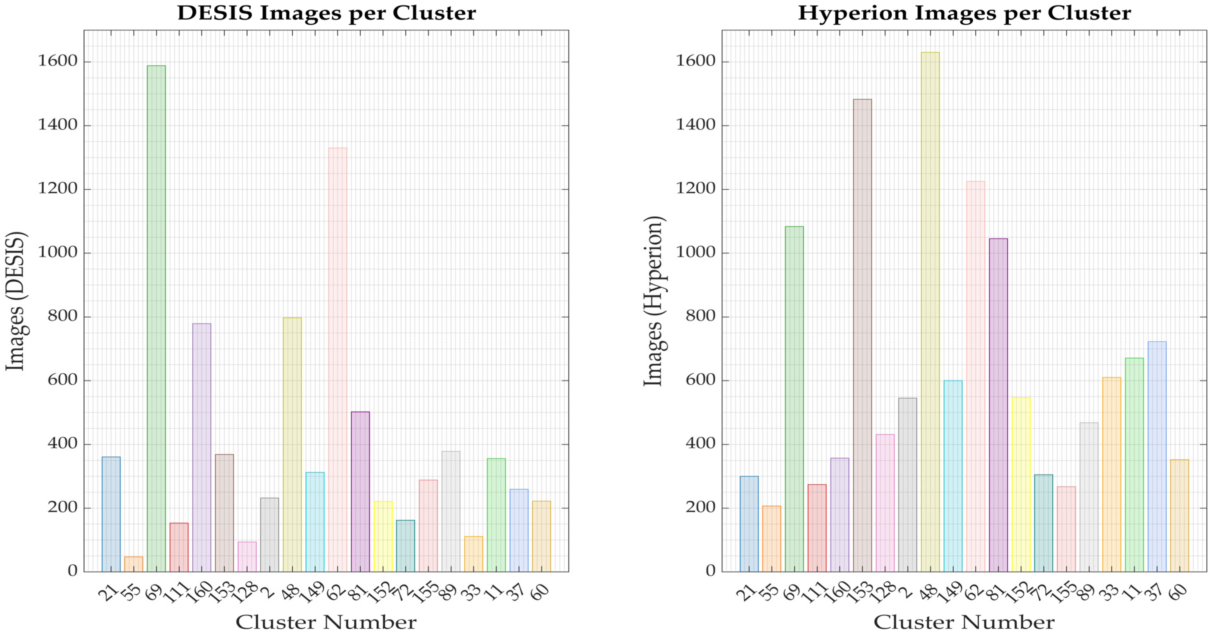
2.1. Selection of Optimal EPICS from Global Land Cover Clustering Analysis

As previously mentioned, Fajardo et al. [16] conducted a global land cover clustering analysis focused exclusively on temporally stable pixels to identify potential global EPICS. This analysis built on an earlier study by Fajardo et al. [24], which performed a per-pixel global stability assessment using various statistical tests to create a global mosaic of temporally stable pixels suitable for radiometric calibration. However, that initial study did not classify the stable pixels by land cover type or into specific spectral classes to identify calibration targets based on spectral characteristics. Building on this foundation, Fajardo et al. [16] used the global mosaic of stable pixels as a baseline and pre-filter in a new clustering analysis, grouping the temporally stable pixels into clusters with similar spectral characteristics using a k-means clustering algorithm.

To conduct this clustering analysis, the authors created data cubes from Landsat 8 Operational Land Imager OLI data, covering each 1° by 1° geographic grid between latitudes −43 and 43 and longitudes −180 and 180. Each data cube contained the temporal mean and standard deviation of TOA reflectance values from 2013 to 2022 across visible, near-infrared (VNIR), and short-wave infrared (SWIR) bands. After filtering with the global mosaic of stable pixels, only the most temporally stable pixels were retained. This filtered data served as input for the k-means clustering algorithm, which assigned each temporally stable pixel to 1 of 160 potential clusters based on temporal and spatial characteristics. The authors also presented the spectral response curves for these 160 clusters using Landsat 8 bands, including Coastal Aerosol, Blue, Green, Red, NIR, SWIR 1, and SWIR 2. Some of the resulting clusters exhibited substantial temporal standard deviations and were excluded as potential EPICS candidates. Based on a temporal standard deviation threshold of less than 0.06—set according to the 3-sigma range observed in previously identified EPICS with various spectral characteristics [15,23]—75 potential EPICS were identified.

To manage this large dataset, refine the selection based on temporal and spectral characteristics, and identify 20 potential EPICS for which spectral profiles were derived in this work; the initial set of clusters identified by Fajardo et al. [16] was further divided using a k-means clustering algorithm. This process resulted in 20 distinct groups. Each group was formed by aggregating the original clusters based on their spectral characteristics through the k-means, aiming to group similar clusters that likely represent comparable land cover types and ensuring a broad dynamic range among the potential EPICS. Within each of these 20 groups, the cluster with the smallest temporal standard deviation across all bands was selected as the optimal EPICS for that group. This approach ensured that each of the 20 chosen EPICS exhibited the most stable characteristics within its group. To verify that the optimal cluster within each group was indeed the best choice, and this process was repeated iteratively 1000 times. The final set of 20 EPICS comprises those that were selected most frequently within each group.

2.2. Data Collection

2.2.1. Earth Observing-1 (EO-1) Hyperion

The Earth Observing-1 (EO-1) satellite was launched from Vandenberg Air Force Base on 21 November 2000, as part of NASA’s New Millennium Program. This satellite is equipped with several advanced instruments, including the Advanced Land Imager (ALI), the Linear Etalon Imaging Spectral Array (LEISA), the Atmospheric Corrector (LAC), and the Hyperion Imaging Spectrometer. Hyperion is notable for being the first high spatial resolution imaging spectrometer in orbit, providing imagery across 196 calibrated spectral bands. It offers a spectral resolution of 10 nm from 400 to 2500 nm, with a spatial resolution of 30 m and a swath of 7.7 by 100 km. These capabilities enable Hyperion to deliver detailed hyperspectral data for a wide range of Earth observation applications [25,26]. This sensor was operational until 2017 when it was decommissioned in March of that year.

The Image Processing Laboratory (IP LAB) holds in its archive all images collected by the Hyperion sensor over its lifetime over North Africa, the RadCalNet site used in this study, and parts of Asia. Figure 1 shows all the locations where hyperspectral data are available and used for this study.

2.2.2. DLR Earth Sensing Imaging Spectrometer (DESIS)

The German Aerospace Center’s Earth Sensing Imaging Spectrometer (DESIS), launched in June 2018 aboard the International Space Station (ISS), is a pushbroom hyperspectral imaging system developed in collaboration with Teledyne Brown Engineering. DESIS captures data across 235 spectral bands in the 400–1000 nm range with a spectral resolution of 2.55 nm. It has a ground sample distance of 30 m and a swath width of 30 km, with a field of view of 4.4 degrees. Operating from the ISS at an altitude of approximately 405 km, DESIS provides observations from 55°N to 52°S latitudes [27].

The IP LAB holds all the L1C data collected by DESIS since its launch until November of 2023 between 36°N and 15°N latitude and 18°W to 35°E longitude over North Africa, and data collected over the RadCalNet sites used for this study as shown in Figure 1.

2.3. Data Processing

2.3.1. EPICS Zonal Masks for EPICS Processing

The output of the global land cover clustering achieved by Fajardo et al. [16] consists of binary continental-scale mosaics, where ones represent pixels identified as part of the same cluster. To enhance data processing efficiency, smaller, more localized masks were created for each location for each sensor and used to retrieve the mean TOA reflectance for each cluster across all sensors employed in this study.

Figure 2 illustrates the continental mosaic output of Cluster 69 over North Africa from Fajardo et al.’s [16] global land cover clustering. In this figure, purple pixels indicate EPICS pixels. Additionally, the figure shows the created binary mask for a DESIS tile located at latitude 28 longitude 23. Green pixels in this mask represent EPICS pixels belonging to Cluster 69 and extracted from the continental mosaic. This mask (green) was subsequently used to retrieve the TOA reflectance of the EPICS pixels at that location.

The masks were generated using GDAL, an open-source geospatial library for reading and writing raster and vector data formats [28]. Each mask was specifically designed to align with the spatial resolution and projection systems of the sensors used in this study.

2.3.2. TOA Reflectance Retrieval of Hyperspectral Data

Mean TOA reflectance of Hyperion was retrieved using Equation (1).

$${\rho }_{\lambda TOA}={\displaystyle \frac{\frac{{DN}_{Cal}}{h}\times \pi \times d^2}{E_{sun}\times sin\varphi \times cos\theta }}$$

(1)

where ${DN}_{Cal}$ represents the calibrated digital number (DN) of the pixel, $h$ is the scaling factor, $d^2$ denotes the Earth-to-Sun distance measured in astronomical units (AU), $E_{sun}$ is the radiance calibration converted to reflectance using the Thuillier’s solar spectrum, $\varphi$ is the solar elevation angle, and $\theta$ is the sensor’s viewing angle [26].

On the other hand, mean TOA reflectance of DESIS was estimated using Equation (2).

$${\rho }_{\lambda TOA}={\displaystyle \frac{ \pi L_{TOA}{d}^2}{\mathit{cos}SZAE0}}$$

(2)

where $L_{TOA}$ is the DESIS-measured radiance, $d$ is the Earth-to-Sun in astronomical units, E0 represents the solar spectral irradiance from Thuillier’s model, and $SZA$ is the solar zenith angle [29].

2.3.3. Cloud Filtering and Outlier Rejection

Unlike sensors such as Landsat or Sentinel, Hyperion and DESIS do not provide pre-defined products or masks for directly removing pixels contaminated by clouds. However, due to the hyperspectral nature of these sensors, measurements in absorption regions can be used to identify clouds. In this study, cloud masks for both DESIS and Hyperion were derived using atmospheric transmittance, as shown in Figure 3, following the methodology in the study performed by Monali Adrija [30]. The authors indicate that transmittance is influenced by various atmospheric molecules, including aerosols such as smoke and dust, as well as gasses like carbon dioxide and water vapor. The water vapor absorption regions were specifically used to develop the cloud filtering masks for these hyperspectral sensors.

As previously mentioned, DESIS has a spectral resolution of 2.55 nm in the 400 to 1000 nm range. Given this, the region between 900 and 1000 nm was selected to identify a suitable spectral band for cloud filtering due to its pronounced absorption features in the DESIS spectral range. The band chosen for cloud filtering within this region was 934 nm, as shown by the red dashed line in Figure 3.

In contrast, Hyperion, with a spectral resolution of 10 nm, extends beyond 1000 nm. An important absorption region, from approximately 1300 to 1500 nm, is highly sensitive to atmospheric absorption and is thus suitable for deriving a cloud filter. For Hyperion, the 1386 nm wavelength was selected because it is one of the bands with low transmittance in this region, as shown by the green dashed line in Figure 3.

For generating the cloud binary masks, a threshold approach was implemented. Pixels in DESIS with a TOA reflectance lower than 0.2 were considered cloudy and marked as zero, while those above this threshold were classified as cloud-free. Similarly, for Hyperion, pixels with a TOA reflectance lower than 0.02 were marked as cloudy, and those above this threshold were considered cloud-free and used for the study.

In addition to the cloud filtering, potential outliers may remain; therefore, to ensure that the hyperspectral profiles for each EPICS derived in this work were not affected by outliers, a 3-sigma threshold was used to remove any other potential outliers remaining. An example of this is shown in Figure 4. In this figure, it is possible to see that mainly the Hyperion data have some potential outliers that fall outside of the threshold and therefore are not considered in the hyperspectral profile estimation.

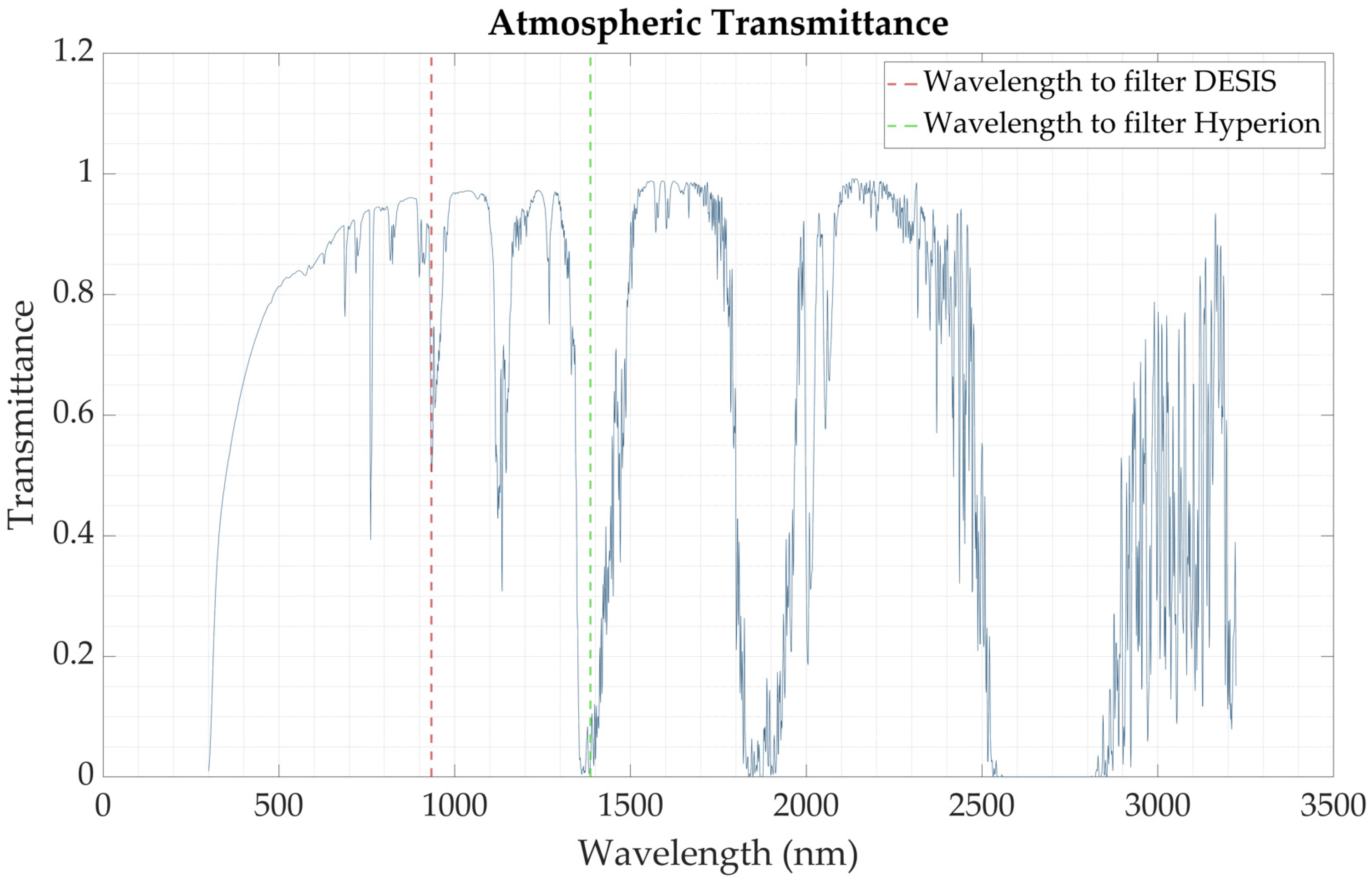
2.3.4. Correction of Hyperspectral Data

Hyperion

The stability of Hyperion was evaluated over the years, for instance, Biggar [31] evaluated the radiometric calibration of Hyperion. The study on Hyperion focused on vicarious radiometric calibration using high-reflectance ground targets. Hyperion, a hyperspectral sensor covering 400 to 2500 nm with 220 spectral bands, was calibrated by referencing ground targets such as Ivanpah Playa and Railroad Valley. The study found that the pre-flight calibration was inconsistent with the sensor’s in-flight performance, revealing a calibration shift of about 8% in the VNIR and 18% in SWIR regions compared to the pre-flight calibration. As a result, new calibration coefficients were adopted in December 2001, which significantly improved the consistency of the data with vicarious calibration results better than 5%.

More recently, Jing et al. [32] aimed to evaluate and correct the lifetime radiometric calibration of the Hyperion sensor. The study analyzed data from the Libya 4 PICS site collected from 2004 until the sensor’s decommissioning in 2017 to detect and correct any temporal drifts in sensor response. Significant drifts were observed in specific bands, notably in bands 8 to 16 and bands 206, 209, and 210. These drifts were corrected, and the corrected data were then validated against ground-based vicarious calibration sites, including those at South Dakota State University (SDSU) and the Radiometric Calibration Network (RadCalNet) Railroad Valley site. The results showed that after applying the drift corrections, the sensor’s calibration was stable across most bands, with statistically significant calibration correction coefficients provided for those that required them. The study also included cross-comparisons with Landsat 7 data, confirming the effectiveness of the drift and calibration corrections. For this study the drift and bias for the radiometric calibration of Hyperion was corrected using the calibration coefficients reported by Jing et al. as follows:

Drift per-year was considered as a linear function of days in a calendar year.

$${\displaystyle \frac{{\%drift}_{\lambda }}{year}}={\displaystyle \frac{{slope}_{\lambda }\ast 365\ast 100}{{intercept}_{\lambda }}}$$

(3)

where the %drift per-year in reflectance is the per-year per-band degradation expressed in percentage, and slope and intercept are the coefficients obtained through a linear regression on the TOA reflectance for each spectral band. With this, the correction of any potential drifts for each band was obtained as follows:

$${\rho }_{\lambda driftCorr}={\rho }_{\lambda }-{\displaystyle \frac{\frac{{\%drift}_{\lambda }}{year}\times Dy}{100}}$$

(4)

where ${\mathit{\rho }}_{\mathit{\lambda }\mathit{c}\mathit{o}\mathit{r}\mathit{r}}$ is the Hyperion drift-corrected mean TOA reflectance, ${\rho }_{\lambda }$ is the Hyperion mean TOA reflectance, and $Dy$ is the decimal year calculated for each collection based on the register overpass time stamp. Finally, the gain and bias correction is applied using Equation (5) and the calibration coefficients obtained by Jing et al.

$${\rho }_{corrected}={gain}_{\lambda }\ast {\rho }_{\lambda driftCorr}+{bias}_{\lambda }$$

(5)

where ${gain}_{\lambda }$ and ${bias}_{\lambda }$ are the calibration coefficients for each spectral band, and ${\rho }_{corrected}$ is the Hyperion drift gain and bias-corrected mean TOA reflectance.

DESIS

The radiometric calibration of DESIS was reported by Alonso et al. [29]. The authors performed the radiometric calibration of DESIS through a combination of vicarious calibration and cross-calibration techniques including the Committee on Earth Observation Satellites (CEOS) PICS and the RadCalNet sites. These ground sites enabled accurate updates to the radiometric coefficients and minor adjustments to the spectral characterization of the sensor. In addition, the DESIS instrument underwent cross-calibration with well-calibrated sensors like Landsat 8 and Sentinel-2. This ensured that DESIS data maintained consistency and accuracy when compared to other satellite measurements

However, a recent study by Monali Adrija et al. [30] identified temporal changes in the mean TOA reflectance of DESIS over an EPICS known as Cluster 13-GTS, previously identified by Fajardo et al. [16]. The authors assessed the temporal stability of the EPICS using Landsat 7 and Landsat 8 data for a temporal evaluation between 1999 and 2024 to rule out any site-related changes, confirming that the observed variations were due to DESIS’s response.

Due to the changes in DESIS, the authors developed a detailed methodology to perform vicarious absolute calibration of DESIS, correcting for temporal changes seen in that same study. First, the authors developed a temporal de-trending model to address sensor-specific drift observed over a stable reference site, Cluster13-GTS, which showed temporal changes attributable to sensor degradation rather than actual target changes. A fourth-order polynomial regression model was selected for temporal correction after testing four potential models (linear, exponential, and second- and fourth-order polynomials). The fourth-order polynomial was chosen based on statistical criteria, residual standard error, F-statistics, p-values, and coefficient significance, showing the best fit for the temporal trend observed.

The polynomial de-trending model is expressed as follows:

$${\rho }_{\lambda ,predicted}={\beta }_0+{\beta }_{1}X+{\beta }_2{X}^2+{\beta }_3{X}^3+{\beta }_4{X}^4$$

(6)

where ${\beta }_0$ to ${\beta }_4$ are model coefficients, ${\rho }_{\lambda ,predicted}$ is the predicted TOA reflectance, and X is the decimal year since launch. The temporal de-trended reflectance ${\rho }_{\lambda ,tempDESIS}$ was then calculated as follows:

$${\rho }_{\lambda ,tempDESIS}={\displaystyle \frac{{\rho }_{\lambda ,reference}}{{\rho }_{\lambda ,predicted}}}\times {\rho }_{\lambda ,BRDF Normalized DESIS}$$

(7)

where ${\rho }_{\lambda ,reference}$ is the reflectance at launch and ${\rho }_{\lambda ,BRDF Normalized DESIS}$ is the BRDF-normalized data.

For absolute calibration, the RadCalNet sites were used as ground truth. DESIS data were filtered to match RadCalNet acquisition geometry, keeping view zenith angles below 11° to limit BRDF-induced error to 1%. The absolute calibration was performed by calculating a gain factor using a Monte Carlo simulation with 1000 iterations, applying weighted 1:1 linear regression on DESIS and RadCalNet data. The absolute corrected reflectance, ${\rho }_{\lambda ,absDESIS}$, was determined by the following:

$${\rho }_{\lambda ,absDESIS}={\rho }_{\lambda ,tempDESIS}\ast gain$$

(8)

where gain is the calibration factor derived from the Monte Carlo simulation and ${\mathit{\rho }}_{\mathit{\lambda },\mathit{a}\mathit{b}\mathit{s}\mathit{D}\mathit{E}\mathit{S}\mathit{I}\mathit{S}}$ is the absolute corrected reflectance used in this study for the estimation of hyperspectral profiles of the different EPICS.

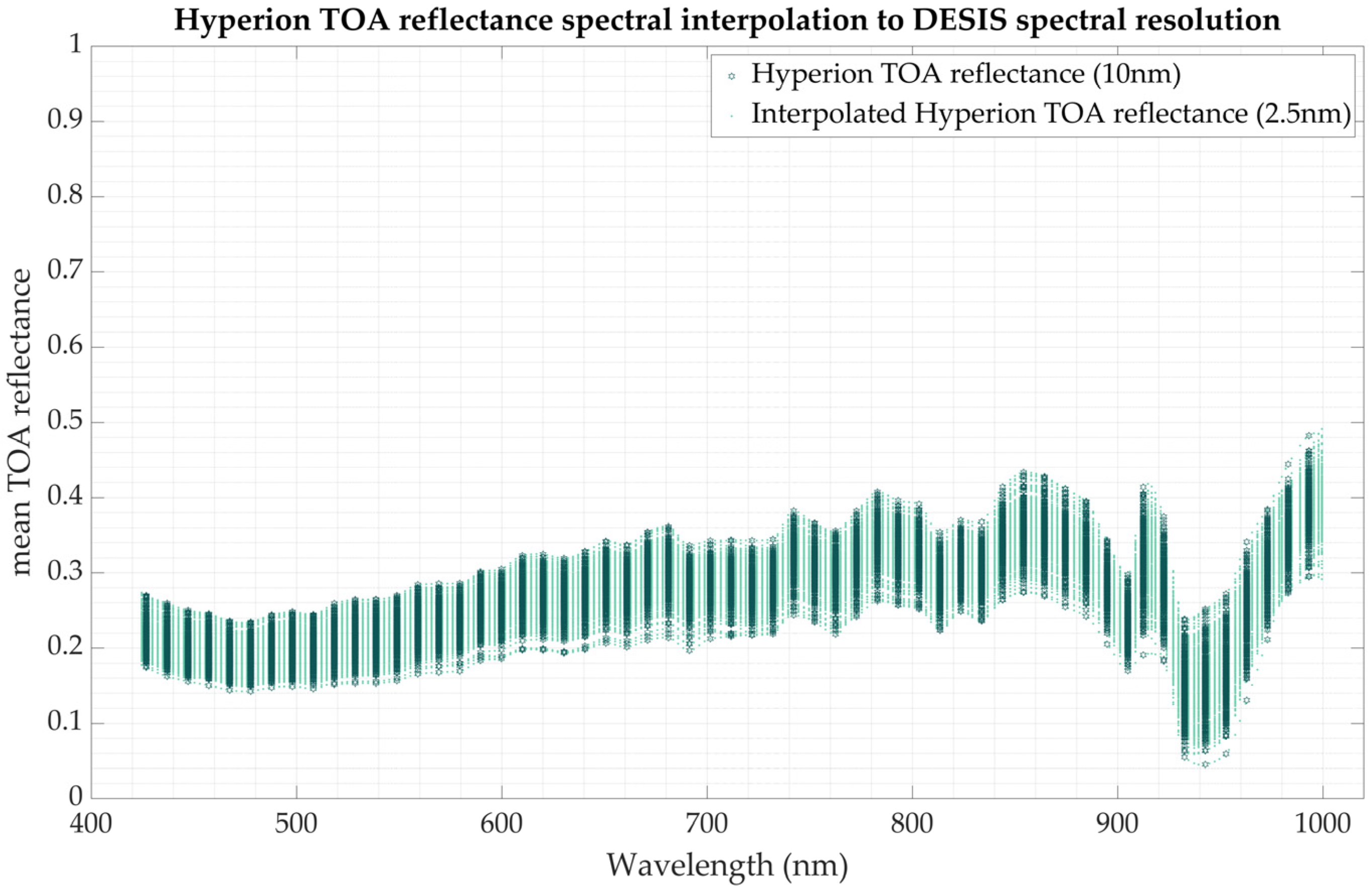
2.3.5. Spectral Interpolation of Hyperion Data

Considering that DESIS and Hyperion have different spectral resolutions, with DESIS having a finer resolution of 2.5 nm compared to Hyperion’s 10 nm, spectral interpolation was performed on the Hyperion data to match DESIS’s spectral resolution over the 425 to 1000 nm range and be able to combine both datasets for the EPICS hyperspectral profile generation. This interpolation was achieved using a modified Akima cubic Hermite method (MAKIMA). The interpolated reflectance values were obtained through a piecewise polynomial function of three degrees. This method provides smooth interpolation that preserves monotonicity and reduces overshoots [23]. This interpolation was performed to the Hyperion TOA reflectance of all 20 EPICS considered in this study. An example of this interpolation can be seen in Figure 5. The dark green data shows the mean TOA reflectance over Cluster 160 from the global land cover clustering retrieved from all locations available in the IP LAB archive that intercepted with this cluster, and the light green data are the Hyperion spectrally interpolated to match the 2.5 nm DESIS spectral resolution used later for the hyperspectral profile derivation. This was carried out for all of the EPICS for the VNIR bands.

2.4. BRDF Normalization

For satellite sensor data, seasonal effects driven primarily by the sun’s position throughout the year can impact reflectance from different targets due to variations in acquisition geometry. This is described by the Bidirectional Reflectance Distribution Function (BRDF). To address this seasonality effect in the mean TOA reflectance of the sensors used in this study, a BRDF model incorporating solar and view geometries developed by Farhad et al. [33] was used. This model accounts for the quadratic behavior of the BRDF, as detailed by Shrestha et al. [34], and transforms the view and solar angles from spherical to linear Cartesian coordinates, providing a TOA reflectance of the surface as a continuous function of independent variables. Kaewmanee et al. [35] further enhanced this BRDF model by adding an interaction term, extending Farhad’s model for a more accurate estimate. The final BRDF model used in this study is as follows:

$$\begin{array}{c}{\rho }_{predicted}={\beta }_0+{\beta }_1{X}_1+{\beta }_2{Y}_2+ {\beta }_3{X}_2+ {\beta }_4{Y}_2+ {\beta }_5{X}_1{Y}_1+{\beta }_6{X}_1{X}_2+{ \beta }_7{X}_1{Y}_2+{\beta }_8{Y}_1{X}_2+{\beta }_9{Y}_1{Y}_2\\ +{\beta }_{10}{X}_2{Y}_2+{\beta }_{11}{X_1}^2+{\beta }_{12}{Y_1}^2+{\beta }_{13}{X_2}^2+{\beta }_{14}{Y_2}^2\end{array}$$

(9)

In this model, $X_1$, $X_2$, $Y_1$, $Y_2$ represent the Cartesian coordinates derived from the spherical coordinates. The coefficients ${\beta }_{0\text{–}14}$ are the coefficients in the model, and ${\rho }_{predicted}$ indicates the predicted TOA reflectance. The Cartesian coordinates used in the development of the model are as follows:

$$X_1=\sin \left(SZA\right)\ast \cos \left(SAA\right)$$

(10)

$$Y_1=\sin \left(SZA\right)\ast \sin \left(SAA\right)$$

(11)

$$X_2=\mathit{sin}\left(VZA\right)\ast \mathit{cos}\left(VAA\right)$$

(12)

$$Y_1=\mathit{sin}\left(VZA\right)\ast \mathit{sin}\left(VAA\right)$$

(13)

where $(VZA$) and $\left(VAA\right)$ refer to the view zenith and azimuth angles, while $\left(SZA\right)$ and $\left(SAA\right)$ denote the solar zenith and azimuth angles.

With this, the BRDF-normalized TOA reflectance is calculated using the following equation:

$${\rho }_{BRDF Normalized}={\displaystyle \frac{{\rho }_{observed}}{{\rho }_{predicted}}}\ast {\rho }_{reference}$$

(14)

where the ${\rho }_{reference}$ is the reference TOA reflectance estimated as the mean TOA reflectance for all spectral bands for each of the 20 EPICS considered in this study. This ensures that the data are normalized to a reference reflectance within each EPICS reflectance range. In addition, ${\rho }_{observed}$ is the sensor’s recorded TOA reflectance of the EPICS pixels for a given day, while the ${\rho }_{predicted}$ is the mean TOA reflectance predicted by the BRDF model for the same day. The BRDF model generated for each EPICS in this study was generated based on the aggregation of both Hyperion and DESIS data for a global single BRDF model of the target, where the shorter wavelengths (VNIR) are comprised by the fusion of Hyperion and DESIS data, whereas the longer wavelength SWIR regions of the electromagnetic spectrum were estimated using hyperion data due to the fact that DESIS only covers the range from 400 to 1000 nm.

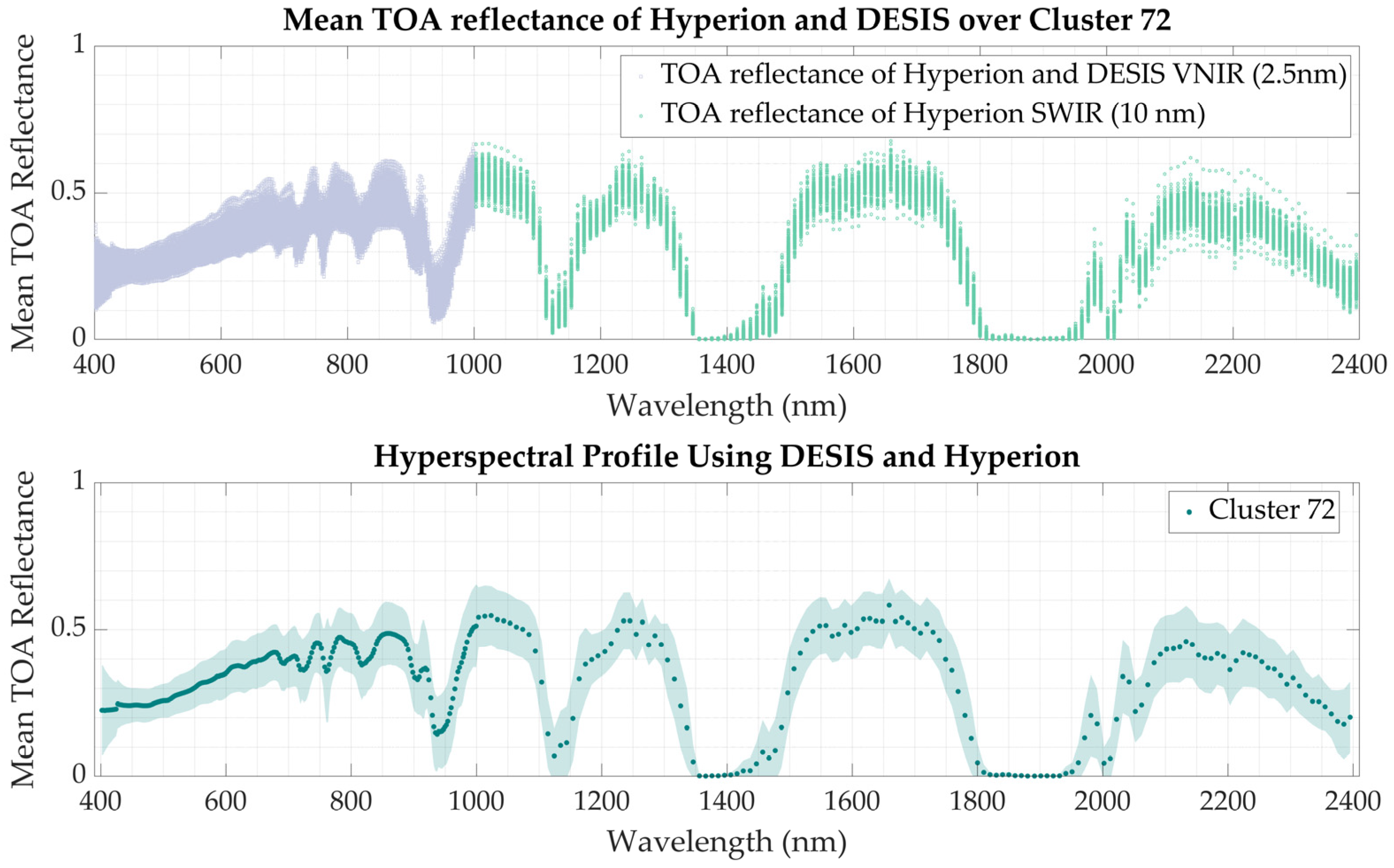
2.5. EPICS Hyperspectral Profile Estimation

For each of the 20 EPICS selected in this study, a hyperspectral profile representing the target’s spectral signature was derived by averaging all hyperspectral observations collected over time from all available locations in the IP LAB archive for each EPICS clusters. For the visible region VIS (400 to 425 nm), DESIS was used, in addition, for the VNIR region (426 nm to 1000 nm), the hyperspectral profile was obtained using both the DESIS data collected for each EPICS and the spectrally interpolated Hyperion data for the same range (2.55 nm). For longer wavelengths (1001 nm to 2400 nm), only the Hyperion data at its native spectral resolution were used, as it was the sole hyperspectral data source available for this region in the study. An example of this can be seen in Figure 6. The top chart illustrates the BRDF-normalized mean TOA reflectance of DESIS and Hyperion for the 400 to 1000 nm range (blue), as well as Hyperion data from 1000 nm to 2400 nm (green). The bottom chart displays the hyperspectral profile derived from the data collected by these sensors over Cluster 72.

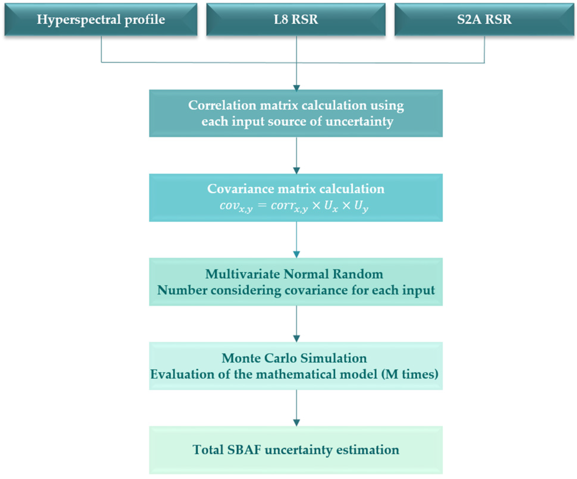
2.6. EPICS Hyperspectral Profile Uncertainty Estimation

To estimate the uncertainty in the hyperspectral profiles derived in this work, the Guide to the Expression of Uncertainty in Measurement (ISO-GUM) methodology was applied. The sources of uncertainty in this analysis include the temporal and spatial variability of the site ${U^2}_{temporal-spatial}$, quantified as the temporal coefficient of variation (CV). This CV is defined as the ratio of the temporal standard deviation to the temporal mean of the TOA reflectance, based on data collected by DESIS and Hyperion over the EPICS in this study. Additional sources include the BRDF ${U^2}_{BRDF}$, which captures the difference between observed and predicted TOA reflectance while accounting for seasonal effects, calculated as the Root Mean Square Error (RMSE) as well as sensor-related uncertainties, ${U^2}_{DESIS}$ and ${{+U}^2}_{Hyperion}$.

In the 400 to 425 nm range, DESIS was the only sensor used; therefore, only DESIS uncertainty is included in Equation (15). For the 425 to 1000 nm range, both DESIS and Hyperion were used, so uncertainties from both sensors are incorporated into the calculation for Equation (16). For the SWIR channels beyond 1000 nm, Hyperion was the only source of hyperspectral data, and thus only Hyperion’s uncertainty is considered for that part of the spectrum in Equation (17). The absolute calibration accuracy of Hyperion is reported at 5% [36], while DESIS has an estimated absolute calibration range of 2.5–5%, with slightly higher uncertainties noted in the absorption wavelength bands [30].

$${\mathrm{U}}_{\mathrm{t}\mathrm{o}\mathrm{t}\mathrm{a}{\mathrm{l}}_{\mathrm{V}\mathrm{I}\mathrm{S}}}\sqrt{{{\mathrm{U}}^2}_{\mathrm{t}\mathrm{e}\mathrm{m}\mathrm{p}\mathrm{o}\mathrm{r}\mathrm{a}\mathrm{l}-\mathrm{s}\mathrm{p}\mathrm{a}\mathrm{t}\mathrm{i}\mathrm{a}\mathrm{l}}+{{\mathrm{U}}^2}_{\mathrm{B}\mathrm{R}\mathrm{D}\mathrm{F}}+{{\mathrm{U}}^2}_{\mathrm{D}\mathrm{E}\mathrm{S}\mathrm{I}\mathrm{S}}}$$

(15)

$${\mathrm{U}}_{\mathrm{t}\mathrm{o}\mathrm{t}{\mathrm{a}\mathrm{l}}_{\mathrm{V}\mathrm{N}\mathrm{I}\mathrm{R}}}\sqrt{{{\mathrm{U}}^2}_{\mathrm{t}\mathrm{e}\mathrm{m}\mathrm{p}\mathrm{o}\mathrm{r}\mathrm{a}\mathrm{l}-\mathrm{s}\mathrm{p}\mathrm{a}\mathrm{t}\mathrm{i}\mathrm{a}\mathrm{l}}+{{\mathrm{U}}^2}_{\mathrm{B}\mathrm{R}\mathrm{D}\mathrm{F}}+{{\mathrm{U}}^2}_{\mathrm{D}\mathrm{E}\mathrm{S}\mathrm{I}\mathrm{S}}{{+\mathrm{U}}^2}_{\mathrm{H}\mathrm{y}\mathrm{p}\mathrm{e}\mathrm{r}\mathrm{i}\mathrm{o}\mathrm{n}}}$$

(16)

$${\mathrm{U}}_{\mathrm{t}\mathrm{o}\mathrm{t}\mathrm{a}{\mathrm{l}}_{\mathrm{S}\mathrm{W}\mathrm{I}\mathrm{R}}}\sqrt{{{\mathrm{U}}^2}_{\mathrm{t}\mathrm{e}\mathrm{m}\mathrm{p}\mathrm{o}\mathrm{r}\mathrm{a}\mathrm{l}-\mathrm{s}\mathrm{p}\mathrm{a}\mathrm{t}\mathrm{i}\mathrm{a}\mathrm{l}}+{{\mathrm{U}}^2}_{\mathrm{B}\mathrm{R}\mathrm{D}\mathrm{F}}+{{\mathrm{U}}^2}_{\mathrm{H}\mathrm{y}\mathrm{p}\mathrm{e}\mathrm{r}\mathrm{i}\mathrm{o}\mathrm{n}}}$$

(17)

2.7. Hyperpectral Profile Validation Methodology

The hyperspectral profile validation methodology consisted of three stages. The first stage involved validating the hyperspectral profile for one of the clusters derived in this work, specifically the GONA-EPICS cluster, where pixels intersected with the RadCalNet Gobabeb (RadCalNet GONA) ROI.

The second stage focused on validating the SBAFs derived from the hyperspectral profile of the GONA-EPICS cluster generated in this work by comparing it to the SBAFs derived directly from the RadCalNet GONA site. SBAF was calculated using a Monte Carlo simulation for three hyperspectral profiles in this comparison: the hyperspectral profile of the RadCalNet GONA site (10 nm), the hyperspectral profile of GONA-EPICS derived using both Hyperion and DESIS data (2.55 nm for VNIR and 10 nm for SWIR), and the hyperspectral profile of GONA-EPICS using only Hyperion data (10 nm). This comparison aimed not only to assess whether the SBAFs derived from the hyperspectral profile of the EPICS is statistically the same as that measured on the ground but also to examine the impact of enhanced spectral resolution—from Hyperion’s 10 nm to DESIS’s 2.55 nm—on SBAF estimation.

The final stage assessed applicability, demonstrating the potential of the EPICS derived by Fajardo et al. [16] and the hyperspectral profiles generated in this work for cross-calibrating Landsat 8 and Sentinel-2A. Results from this stage were then compared to cross-calibration outcomes achieved using traditional PICS, such as Libya 4, with Hyperion serving as the hyperspectral data source, as was traditionally conducted.

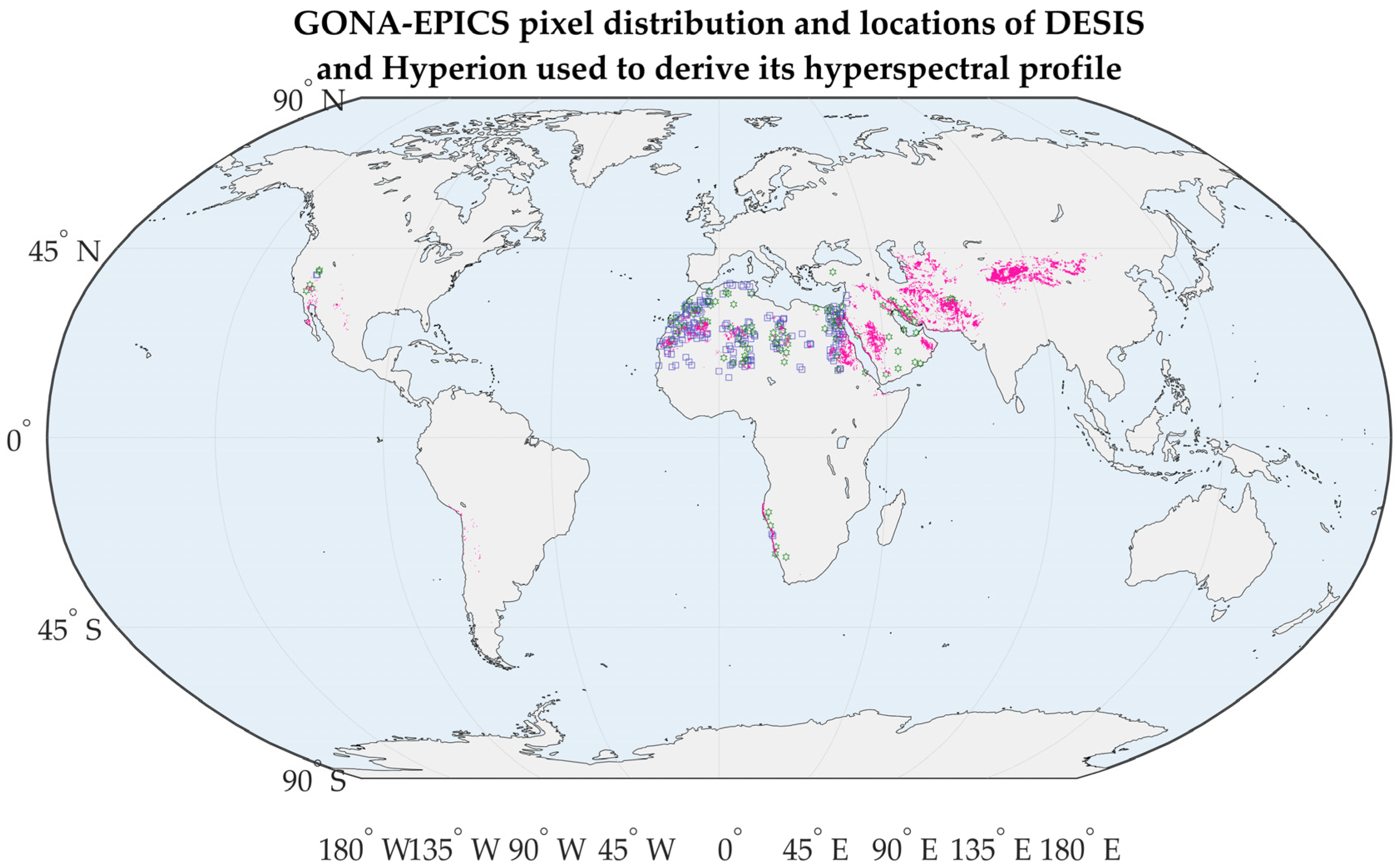
2.7.1. Hyperspectral Profile Validation Targets

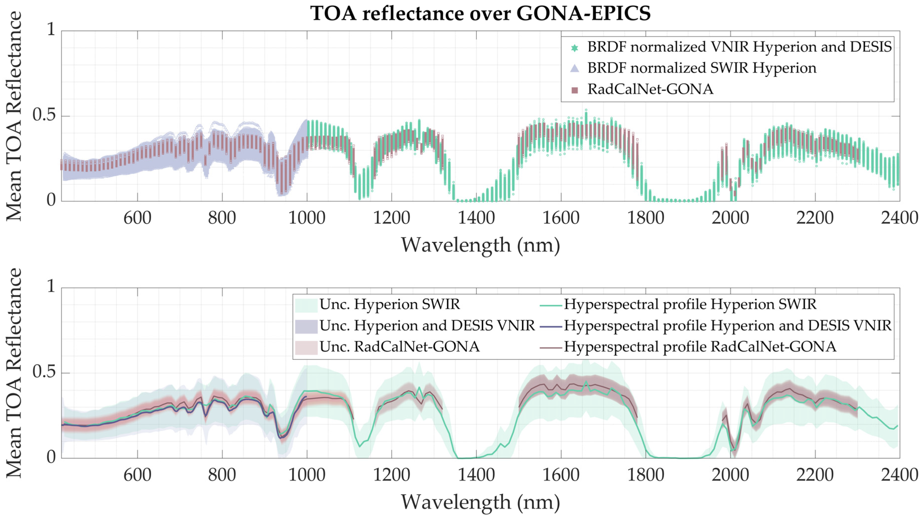
GONA-EPICS

Figure 7 shows the distribution of scenes used to derive this hyperspectral profile, along with the global distribution of GONA-EPICS pixels, shown in magenta. As previously mentioned, this cluster was selected because it includes pixels that overlap with the RadCalNet GONA site. Most of the DESIS and Hyperion images in the IP LAB archive used in this study were collected over North Africa. For the derivation of the GONA-EPICS hyperspectral profile, a total of 779 scenes from DESIS and 357 scenes from Hyperion were used.

RadCalNet-GONA

RadCalNet, operational since 2018, is a network of automated sites that measure various parameters essential for the radiometric calibration of optical sensors onboard satellites for Earth observation. These sites ensure that radiometric calibrations are traceable to the International System of Units (SI). Data collected at these automated sites is recorded in 30 min intervals for nadir-viewing sensors, with a spectral resolution of 10 nm and a range of 400 nm to 2400 nm for some sites, and from 400 nm to 1000 nm for others [37].

This network comprises five locations: Railroad Valley Playa (RVUS) in the United States, La Crau (LCFR) in France, Gobabeb (GONA) in Namibia, and Baotou (BTCN-BSCN) in China, which contains both artificial and sand targets. For validating the hyperspectral profile of the GONA-EPICS derived in this work, RadCalNet-GONA was chosen as the RadCalNet site for EPICS validation, considering that the GONA-EPICS includes pixels from the RadCalNet-recommended ROI.

The RadCalNet-GONA site in Gobabeb, Namibia, collects measurements every 30 min using an ASD FieldSpec spectroradiometer, which has a spectral range of 400 nm to 2400 nm and a spectral resolution of 10 nm. The TOA reflectance product represents a 30 m radius located at latitude 23.6002°S and longitude 15.11956°E [38,39].

2.7.2. RadCalNet-GONA vs. GONA-EPICS Hyperspectral Signature Validation Methodology

As mentioned earlier, the GONA-EPICS hyperspectral profile was derived from images collected by DESIS and Hyperion over this EPICS on a global scale. Additionally, to evaluate potential differences introduced by including DESIS data, the hyperspectral profile of GONA-EPICS was also computed using only Hyperion scenes.

The validation of GONA-EPICS involved assessing whether the hyperspectral profiles derived in this work—the profile obtained from the combination of DESIS and Hyperion data (2.55 nm for VNIR and 10 nm for SWIR) and the profile derived using only Hyperion scenes (10 nm)—align with the hyperspectral profile obtained from RadCalNet data (10 nm), within their respective uncertainties.

Validation of GONA-EPICS against RadCalNet-GONA at the multispectral level was previously conducted by Fajardo et al. [16], who used RadCalNet-GONA data collected at 9 UTC and Landsat 8. Their study indicated that the mean TOA reflectance of RadCalNet-GONA and GONA-EPICS was statistically indistinguishable within the EPICS uncertainty. In this work, the same RadCalNet-GONA TOA reflectance was used to validate the hyperspectral profile derived for the EPICS, utilizing the hyperspectral data provided by RadCalNet and its corresponding uncertainty.

Finally, the mean TOA reflectance of the RadCalNet-GONA site was normalized using the same BRDF model generation methodology applied to the EPICS, as described in Section 2.4. This BRDF-normalized mean TOA reflectance of the RadCalNet-GONA site was then averaged to produce a hyperspectral profile for RadCalNet.

Welch’s Test

To evaluate whether the hyperspectral profile of the GONA-EPICS cluster, derived from DESIS and Hyperion data, is statistically equivalent to the RadCalNet GONA ROI hyperspectral profile obtained from ground measurements, a Welch’s test was applied. This test compares two means while taking their associated uncertainties into account.

For a per-band comparison, the RadCalNet profile, with its uniform 10 nm resolution, was used as the reference for the evaluation, as the hyperspectral profile in this study has a spectral resolution of 2.5 nm in the VNIR region and 10 nm in the SWIR region. The GONA-EPICS hyperspectral profile was therefore spectrally interpolated, following the methodology detailed in Section 2.3.5, to match the wavelengths and spectral resolution of the RadCalNet GONA profile. The Welch’s test is as follows [40]:

The hypotheses of Welch’s t-test are the following:

Null Hypothesis:

$$H_0={\mu }_{RCN-GON{A}_{hyperspectral}}={\mu }_{GONA-EPIC{S}_{hyperspectral}}$$

(18)

Alternative Hypothesis:

$$H_1={\mu }_{RCN-GON{A}_{hyperspectral}}\ne {\mu }_{GONA-EPIC{S}_{hyperspectral}}$$

(19)

Welch’s t-test assesses whether the difference between the sample means is statistically significant, taking into account unequal variances—in this case, the uncertainty of each dataset. The t-test is performed between the samples as follows:

$$t={\displaystyle \frac{{\mu }_{RCN-GON{A}_{hyperspectral}}-{\mu }_{GONA-EPIC{S}_{hyperspectral}}}{\sqrt{{U^2}_{RCN-GON{A}_{hyperspectral}}+{U^2}_{GONA-EPIC{S}_{hyperspectral}}}}}$$

(20)

where ${\mu }_{RCN-GON{A}_{hyperspectral}}$ represents the RadCalNet GONA hyperspectral profile, ${\mu }_{GONA-EPIC{S}_{hyperspectral}}$ denotes the GONA-EPICS hyperspectral profile at 10 nm spectral resolution, ${U^2}_{RCN-GON{A}_{hyperspectral}}$ is the reported uncertainty for the RadCalNet GONA profile, and ${U^2}_{GONA-EPIC{S}_{hyperspectral}}$ is the uncertainty associated with the hyperspectral profile derived for this cluster, as described in Section 2.6. The null hypothesis assumes that the two population means are equal; the significance level used in this study is 0.05. The p-value indicates the probability of observing the data, or something more extreme, under the condition that the null hypothesis is true. A p-value higher than the significance level suggests that the observed differences are likely due to random chance rather than a meaningful effect, providing insufficient evidence to reject the null hypothesis.

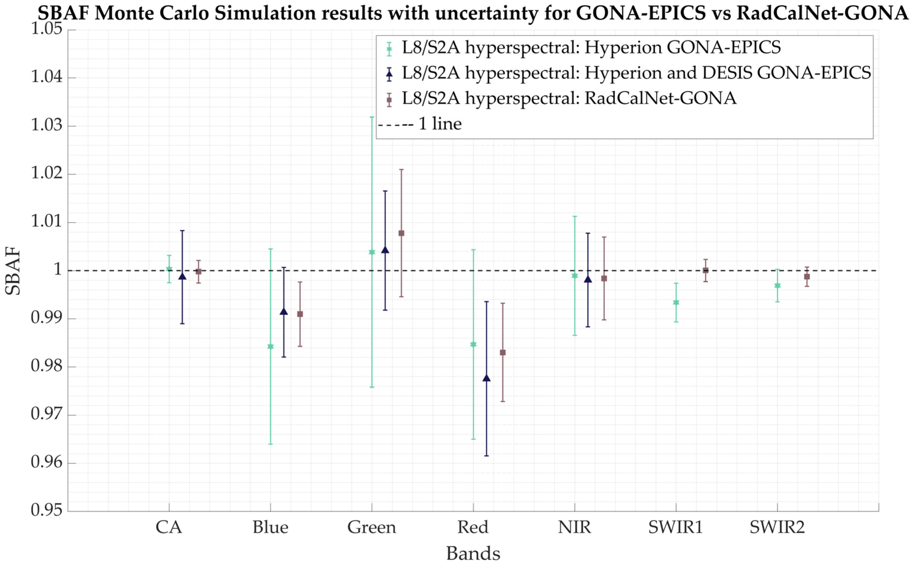
2.7.3. Validation of SBAFs Derived from RadCalNet-GONA vs. GONA-EPICS Methodology

To further validate the applicability of these EPICS and their hyperspectral profiles derived in this work, a comparison was made between the SBAF obtained using the RadCalNet-GONA hyperspectral profile and the SBAF derived from the GONA-EPICS, using Landsat 8 and Sentinel-2A sensors.

SBAF is a crucial element when using data from different platforms and agencies. It is particularly important because even when sensors observe the same target under identical acquisition geometries, the recorded TOA reflectance can vary due to the relative spectral response of each sensor. SBAF accounts for these spectral differences and is essential for cross-calibration efforts, among other applications. SBAF was calculated using Equation (21).

$$SBAF={\displaystyle \frac{{\rho \lambda }_{ref}}{{\rho \lambda }_{cal}}}={\displaystyle \frac{\frac{\int {\rho }_{\lambda h} {RSR}_{\lambda \left(ref\right)}d\lambda }{\int {RSR}_{\lambda \left(ref\right)}d\lambda }}{\frac{\int {\rho }_{\lambda h} {RSR}_{\lambda \left(cal\right)}d\lambda }{\int {RSR}_{\lambda \left(cal\right)}d\lambda }}}$$

(21)

where ${\rho \lambda }_{ref}$ and ${\rho \lambda }_{cal}$ are, respectively, the simulated TOA reflectance for the reference sensor and the sensor to be calibrated; ρλh is the hyperspectral profile of the surface; and ${RSR}_{\lambda \left(ref\right)}$ and ${RSR}_{\lambda \left(cal\right)}$ are the relative spectral responses of the reference sensor and the sensor to be calibrated [19].

For this comparison, the hyperspectral profile of the surface is the GONA-EPICS hyperspectral profile and the RadCalNet-GONA hyperspectral profile. Traditionally, SBAF is calculated by obtaining an SBAF for each observation acquired over time. The final SBAF is then computed as the mean of the individual SBAFs, with the uncertainty represented by the temporal standard deviation of these values [22]. However, in addition to the temporal standard deviation, which captures the variability of the target over time, other sources of uncertainty should be considered. One source is the RSR of the sensors, which also has an associated uncertainty that can impact the overall SBAF uncertainty.

To calculate an SBAF that accounts for both the uncertainty associated with the hyperspectral profiles and the uncertainty of the sensors’ RSRs, the SBAF derived from the GONA-EPICS hyperspectral profile and the RadCalNet-GONA site was estimated using a Monte Carlo simulation approach, as illustrated in Figure 8. In this simulation, the input data includes the hyperspectral profile and the sensors’ RSRs along with their corresponding uncertainties. The RSR for Landsat 8 was obtained from the USGS Spectral Characteristics Viewer (https://landsat.usgs.gov/spectral-characteristics-viewer, accessed on 1 May 2024), while the RSR for Sentinel-2A was downloaded from the Copernicus website (https://sentinels.copernicus.eu/web/sentinel/user-guides/sentinel-2-msi/document-library/-/asset_publisher/Wk0TKajiISaR/content/sentinel-2a-spectral-responses, accessed on 1 May 2024).

Unlike Landsat 8, the Sentinel-2A RSR did not include an associated uncertainty; therefore, for this work, a 5% uncertainty was assigned to Sentinel-2A RSR, in line with the design for absolute radiometric calibration of Sentinel-2A [41,42]. Figure 9 illustrates the input to the Monte Carlo simulation for Cluster 72. The markers represent the sensors’ RSRs and hyperspectral profiles, while the shaded areas indicate the uncertainty associated with each input parameter. For the Monte Carlo simulation, the probability density function (PDF) of the input quantities is necessary to propagate uncertainties through the mathematical model, which in this case is the SBAF.

Teixeira Pinto et al. [43] demonstrated that correlation can significantly impact the final uncertainty of the SBAF. In their study, the authors showed that a correlation of zero yields the “worst-case scenario”, resulting in the highest uncertainty, whereas a correlation of one leads to the lowest uncertainty. For this study, a correlation of zero was assumed, as this condition represents the maximum possible uncertainty thereby minimizing the risk of underestimating uncertainty.

The covariance matrix required for generating the PDFs was estimated using the correlation matrix (which has ones on the main diagonal and zeros elsewhere), along with the uncertainties of the RSRs and the hyperspectral profile, as outlined in Figure 8. The PDF of the input variables was then generated, and a Monte Carlo simulation was conducted for 1000 iterations. SBAF and total uncertainty were calculated as the mean of the SBAF values obtained from the Monte Carlo simulation, while the uncertainty was determined by the standard deviation of those SBAF values.

2.8. Cross-Calibration Using Derived SBAF from New Hyperspectral Profiles with EPICS Versus Traditional Cross-Calibration

To evaluate the capabilities of the EPICS, the hyperspectral profiles derived in this work, the SBAF methodology applied in this study, and the potential of the EPICS derived by Fajardo et al. [16], for cross-calibration efforts, the EPICS and hyperspectral profile of a cluster containing the Libya CNES ROI, known as Cluster 13-GTS, were used for comparison. Details about the cross-calibration methodology followed for each target are described in the upcoming subsections.

2.8.1. Traditional Cross-Calibration and Its Uncertainty

In this work, traditional cross-calibration used the Libya 4 CNES ROI as the target. The mean TOA reflectance of Landsat 8 and Sentinel-2A was extracted using the methodology followed by Farhad et al. [33] The temporal mean TOA reflectance obtained from the Libya 4 CNES ROI for both sensors was then BRDF-normalized according to the methodology described in Section 2.4.

For cross-calibration of sensors, it is necessary to adjust for differences in spectral responses; in this case, the RSRs of Landsat 8 and Sentinel-2A. The SBAF was derived following the methodology described in Section 2.7.3, using the hyperspectral profile of the Libya 4 CNES ROI, calculated as the mean TOA reflectance of Hyperion data collected over the same ROI.

To determine the gain between Landsat 8 and Sentinel-2A over this target and following PICSCAR methodology for cross-calibration, BRDF-normalized TOA reflectance data for both sensors were collected for each month within a 6-month interval. The gain for each monthly mean TOA reflectance was estimated as the ratio of Landsat 8 to Sentinel-2A, with Landsat 8 as the reference sensor and Sentinel-2A as the sensor to be calibrated. The 6-month cross-calibration gain was then calculated as the average of these monthly gains. The total cross-calibration gain was determined as the mean of these 6-month gains over the years.

In the traditional cross-calibration method used, the uncertainty of the total gain is estimated as the average of the standard deviations of each 6-month gain over the available period. For example, if two years of data provide four 6-month gains, the uncertainty is calculated as the average of the standard deviations of these four gains [44]. However, this approach does not adhere to the ISO-GUM uncertainty estimation methodology.

2.8.2. EPICS T2T Cross-Calibration and Its Uncertainty

For the cross-calibration of Landsat 8 and Sentinel- 2A using EPICS, Cluster 69 was selected because it includes pixels from the Libya 4 CNES PICS. This EPICS, referred to as Cluster 13-GTS in Fajardo et al. [16], demonstrated significant potential as a calibration and stability monitoring target, providing more than 50 calibration points per Landsat 8 cycle. Therefore, in this work, Cluster 13-GTS was selected as the target for cross-calibration analysis.

The T2T cross-calibration technique is a methodology used for cross-calibration when employing EPICS as targets [18]. This technique allows for daily cross-calibration gain calculation by first normalizing BRDF effects, following the methodology described in Section 2.4. After the BRDF normalization process, the SBAF was applied to the sensor to be calibrated (Sentinel-2A). In this work, the SBAF derived from the hyperspectral profile obtained for Cluster 69 (Cluster 13-GTS), using Hyperion and DESIS data, was used to correct the Sentinel-2A data.

The next step in the T2T methodology involves temporal interpolation and smoothing of the BRDF-normalized TOA reflectance over the EPICS for each sensor, using a modified Savitzky–Golay (MSG) filter. This filter employs a polynomial fitting approach to the time series data, fitting a polynomial of order three within a moving window of 120 days. The resulting trends represent the daily changes in sensor measurements and can be used to evaluate the sensors’ calibrations on a daily basis.

Once the smoothed trends for each sensor are extracted using the MSG filter, the next step in the T2T cross-calibration technique is to calculate the cross-calibration gain. This involves determining the ratio of the trends obtained from the mean TOA reflectance between a reference sensor (Landsat 8) and the sensor to be calibrated (Sentinel-2A). For each day, the gain is computed by dividing the trend of the reference sensor by the trend of the sensor being calibrated. This technique provides a daily measure of the calibration differences between the two sensors. The T2T method can detect discrepancies and variations in sensor calibration over time, enabling more frequent and detailed evaluations of sensor performance. This continuous assessment allows for the identification of calibration drifts and ensures that the sensors remain aligned to a common radiometric scale.

The uncertainty for the cross-calibration of sensors using EPICS and the T2T methodology follows the ISO-GUM methodology. Four sources of uncertainty were considered in computing the uncertainty on the cross-calibration gain obtained using the T2T technique.

The first source of uncertainty is the uncertainty associated with the site, computed as the CV, as mentioned earlier. This CV accounts for both the temporal variability of the site and the potential variability between different portions of the cluster (e.g., Path/Row to Path/Row). Another source of uncertainty considered is the SBAF. In this case, the uncertainty calculated through the Monte Carlo simulation approach, as explained in Section 2.7.3, was used. Additionally, the BRDF uncertainty, calculated as RMSE measuring the difference between the observed and predicted TOA reflectance, was included. Finally, the absolute uncertainty of the reference sensor, Landsat 8, was also considered, with an uncertainty of 3%. The total uncertainty on the gain was computed using Equation (22).

$$U_{total}\sqrt{{U^2}_{temporal-spatial}+{U^2}_{SBAF}+{U^2}_{BRDF}+{U^2}_{sensor}}$$

(22)

3. Results and Analysis

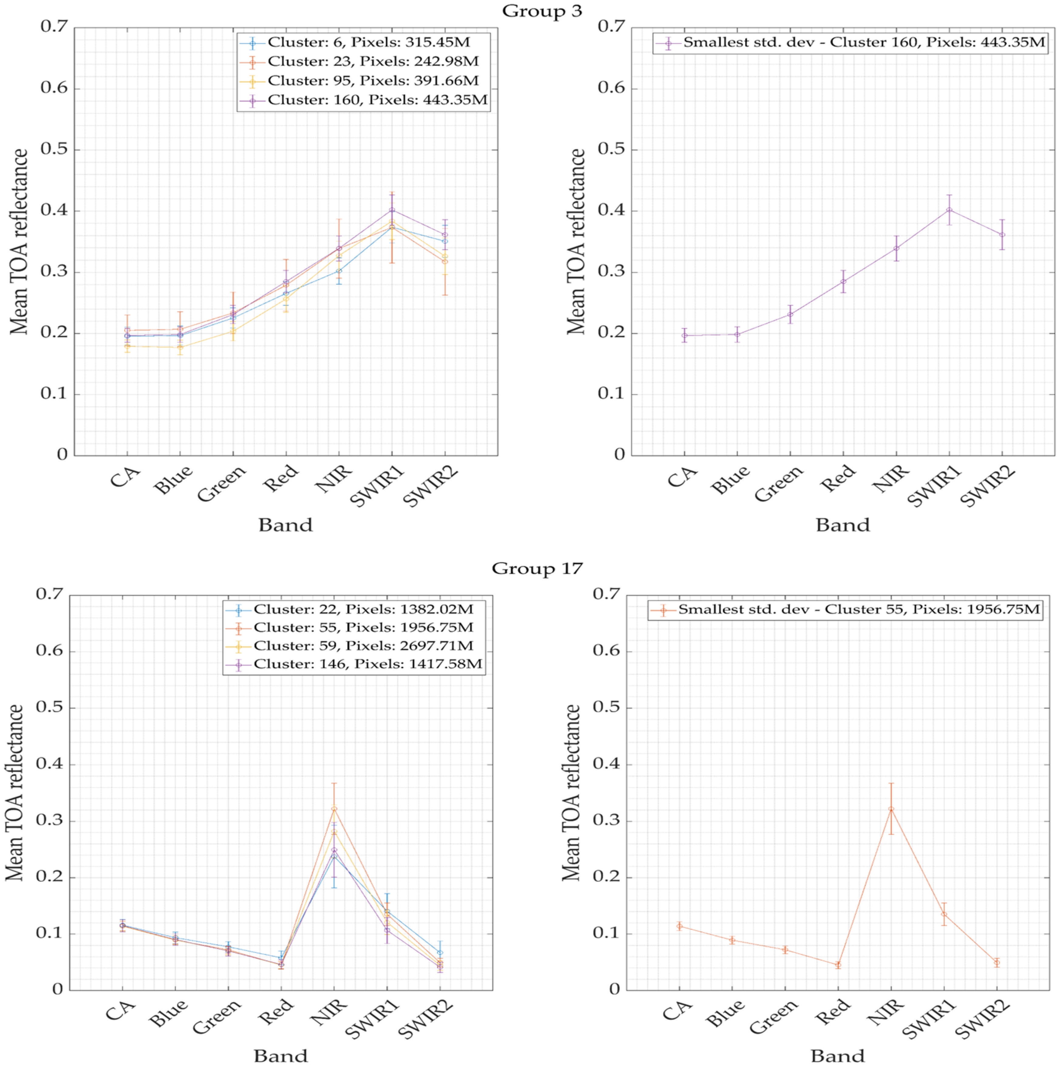
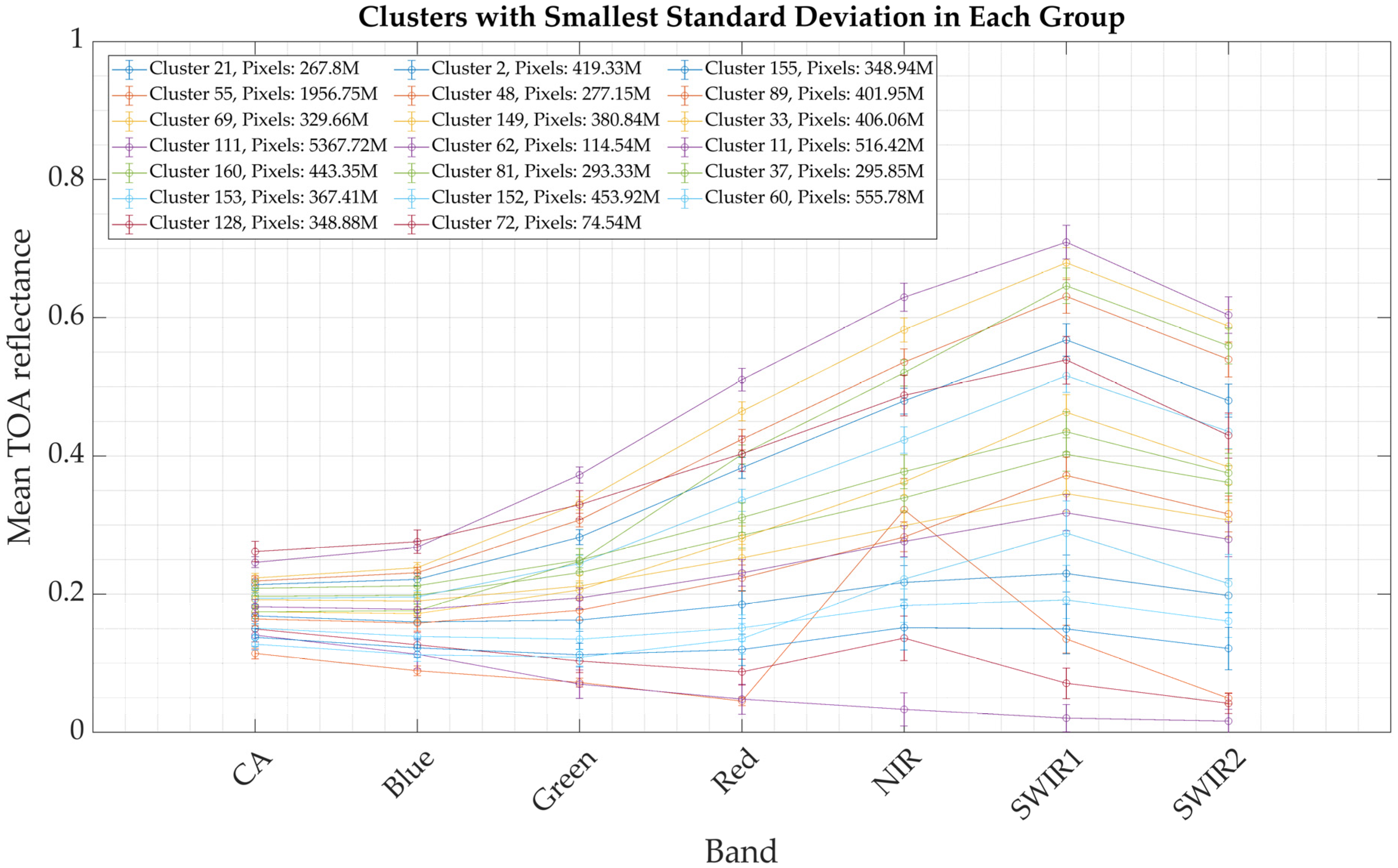
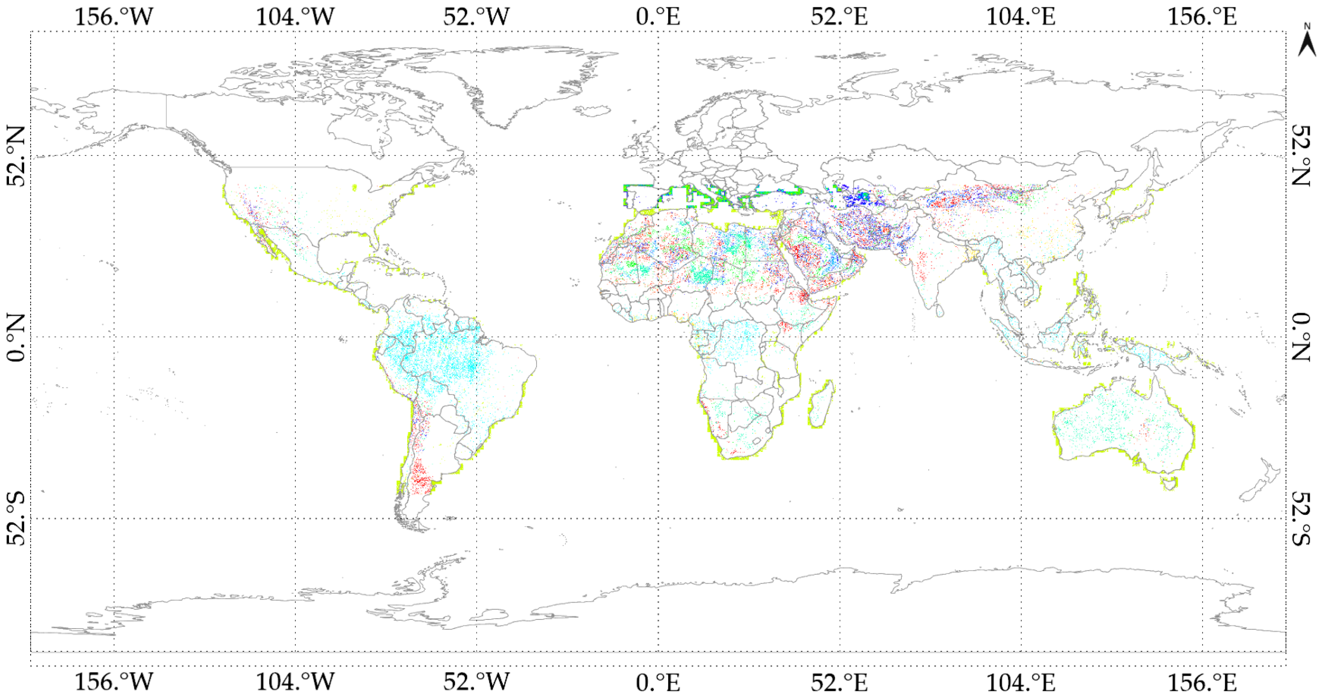
3.1. Results of 20 EPICS Selected

As outlined in Section 2.1, the 75 clusters produced by Fajardo et al.’s [16] global land cover clustering were further divided using a k-means clustering algorithm. This process identified 20 groups of clusters with distinct spectral characteristics. Within each of these 20 groups, clusters with similar spectral properties were grouped together. The cluster within each group that exhibited the smallest temporal standard deviation across all 20 bands was selected as 1 of the 20 EPICS.

Figure 10 provides an example of the results for Group 3 and Group 17. As shown, Clusters 6, 23, 95, and 160 from Group 3 were grouped based on their similar spectral characteristics. Cluster 160 was chosen as the representative cluster due to its smallest temporal variability across all bands. This cluster, which is a sand target with over 443 million pixels, corresponds to the GONA-EPICS cluster reported by Fajardo et al. [16] and includes pixels from the RadCalNet-GONA ROI. Its selection confirms the cluster’s temporal stability and reduced variability compared to other clusters with similar spectral characteristics.

In addition, Group 17 displays a response that aligns with the spectral signature of vegetation. Clusters 22, 55, 59, and 146 were grouped in Group 17 based on their similar spectral characteristics. However, due to its lower temporal standard deviation compared to other clusters in this group, Cluster 55 was selected as the EPICS for Group 17. This cluster, encompassing more than 1.9 billion pixels and spanning South America, Central Africa, East Asia, among others, is likely representative of tropical forests. This assessment was further confirmed by visual inspection.

Figure 11 displays the 20 EPICS multispectral profiles selected based on the grouping described above. These clusters represent various spectral characteristics and exhibit the smallest standard deviation within their respective groups. These EPICS have the potential to serve as calibration targets, providing a global distribution that reduces dependence on single calibration sites and offers a broader dynamic range for radiometric calibration.

In addition, Figure 12 illustrates the pixel distribution of these clusters, showcasing their global coverage. The cluster with the highest number of pixels is Cluster 111, which has over 5.3 billion pixels and represents ocean water around the world, as captured in the data cubes created for coastal regions. Among land representations, Cluster 55 has the highest pixel count, expanding across the Amazon rainforest, central Africa, and East Asia, with over 1.9 billion pixels. Other clusters with significant pixel counts include Cluster 60 with over 500 million pixels representing rock formations around the world in North America, South America, South Africa, and others. Other clusters with a large number of pixels are Cluster 160 with over 440 million pixels and also contains pixels from the RadCalNet-GONA ROI. Conversely, Cluster 72 contains the fewest pixels, with only 74 million pixels in it, representing very bright pixels around the world but mainly in North Africa and Middle East.

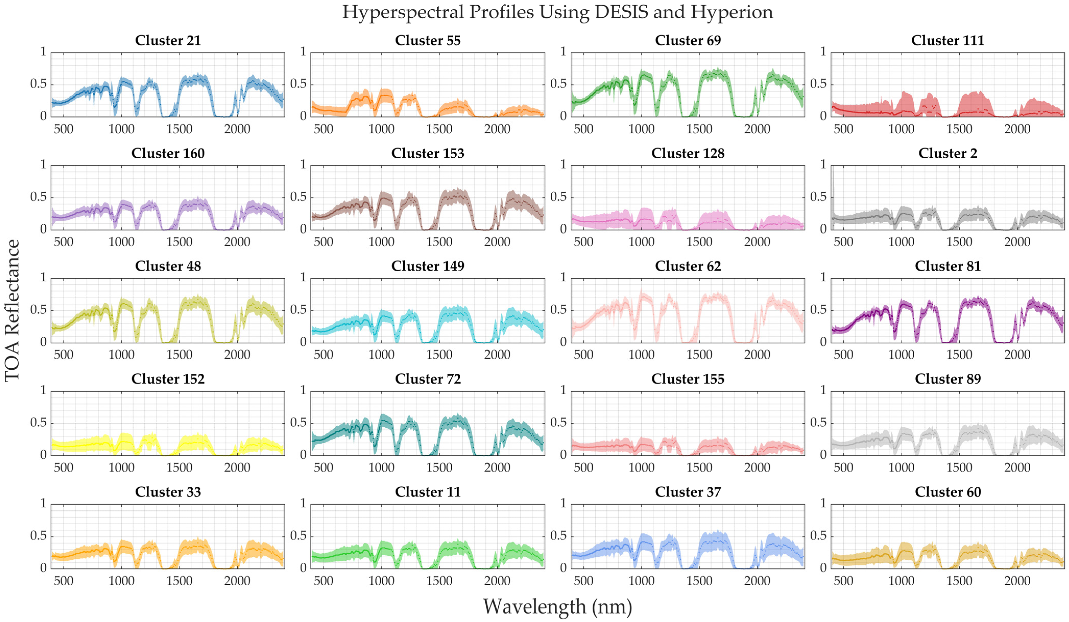
3.2. Hyperspectral Profiles of 20 EPICS

As previously mentioned, several applications, including cross-calibration, require the spectral signature of the target. In this work, and for the first time, the hyperspectral profiles of each of the 20 selected EPICS were estimated. This was achieved using both Hyperion and DESIS data. This new approach not only provides an additional source of hyperspectral information but also enhances the spectral resolution of the resulting signatures due to DESIS’s 2.55 nm resolution in the VNIR region.

For calculating the hyperspectral profiles, the methodology outlined in Section 2.5 was followed. Figure 13 displays the number of observations used for each sensor for each EPICS. Figure 13 (left) shows the number of scenes from DESIS used to derive the hyperspectral profile for the VNIR region. Figure 13 (right) illustrates the scenes from Hyperion, which were used not only for the VNIR region (spectrally interpolated to 2.55 nm) but also for the SWIR regions, as Hyperion was the sole available hyperspectral data source for these bands in this study.

The bar plots illustrate the distribution of DESIS and Hyperion images across the 20 EPICS. In the left plot, which represents the DESIS images used in the analysis, it is evident that Cluster 69 contains the highest number of images, nearly reaching 1600. This is expected, as Cluster 69 includes pixels from the well-known and frequently imaged Libya 4 PICS. Other clusters, such as 160, 48, and 62, also exhibit high image counts, ranging from over 700 to more than 1200 observations. Several clusters, including 21, 153, 149, 89, and 81, show moderate image counts between 200 and 400 scenes. Conversely, clusters like 55, 128, and 33 have notably fewer images, with counts below 150.

The right plot, displaying Hyperion results, shows that Cluster 69 again stands out with the highest image count, around 1600. Clusters 48 and 153 also demonstrate a large number of images, with counts close to 1400. Clusters such as 62, 81, 11, and 37 present substantial counts ranging from 600 to over 1000. In contrast, Clusters 55, 111, and 155 have fewer images, mirroring the pattern observed in the DESIS plot, with counts below 300.

A comparative analysis of both plots reveals a similar trend, with certain clusters like 69, 48, 62, and 81 showing significantly higher image counts. This pattern suggests that these clusters represent spectral characteristics that are prevalent or commonly observed by both sensors, potentially including other PICS. Additionally, the presence of clusters with low image counts, such as 55, 155, and 111, in both sensors indicates these clusters correspond to less frequently observed spectral characteristics, potentially related to vegetation or targets with darker spectral features, such as water.

Figure 14 shows the resulting hyperspectral profiles of the 20 EPICS selected in this work, estimated using DESIS and Hyperion. The shaded area in these hyperspectral profiles represents the uncertainty for each band for each EPICS (3-sigma level). It can be seen that Clusters 62, 69, 21, 81 and 48 are some of the brightest clusters across all bands; these clusters also exhibit smaller uncertainties compared to some of the darkest clusters such as 128, 111, and 152. There are however other clusters such as Cluster 55 and Cluster 2 with dark spectral characteristics but with higher uncertainty. These EPICS hyperspectral profiles are valuable for cross-calibration and absolute model development, offering the advantages of global coverage with a broader dynamic range compared to traditional PICS thus providing multiple alternative targets for the calibration and monitoring of optical satellite sensors.

3.3. Validation Results

3.3.1. RadCalNet-GONA vs. GONA-EPICS

Welch’s Test Results

Figure 15 displays the TOA reflectance and hyperspectral profile of the GONA-EPICS cluster. The top chart illustrates the DESIS and Hyperion data collected across all GONA-EPICS locations, while the bottom chart presents the resulting hyperspectral profile obtained using both DESIS and Hyperion data (2.5 nm for VNIR, 10 nm for SWIR), compared to the RadCalNet-GONA hyperspectral profile (10 nm) and the GONA-EPICS profile derived using only Hyperion data (10 nm).

In the bottom chart, it can be observed that the VNIR portion of the GONA-EPICS hyperspectral profile—derived from the combination of DESIS and Hyperion data—closely follows the RadCalNet-GONA hyperspectral profile, especially in comparison to the profile obtained using only Hyperion data. For longer wavelengths, where the hyperspectral profile was derived solely from Hyperion data, there is a slight divergence between the RadCalNet-GONA and GONA-EPICS profiles; however, they remain within each other’s uncertainties.

To validate whether the RadCalNet GONA hyperspectral profile and the hyperspectral profile of the GONA-EPICS derived in this work are statistically the same, Welch’s test was applied following the methodology described in Section 2.7.2. The top chart in Figure 16 displays the non-absorption coincident bands between RadCalNet GONA mean TOA reflectance and GONA-EPICS mean TOA reflectance at 10 nm spectral resolution. Absorption bands were excluded from this analysis due to their higher uncertainty reported by RadCalNet. The bottom chart shows the p-values from Welch’s test for each band in the top chart, with a horizontal line indicating the significance level of 0.05.

As seen in the bottom chart in Figure 16 displaying the p-values from Welch’s test, the mean TOA reflectance of the GONA-EPICS cluster and the RadCalNet GONA site are statistically the same across most wavelengths (p-value > 0.05), except at 1270 nm, 1990 nm, and 2000 nm, which correspond to bands near absorption feature regions. This indicates that, for the majority of wavelengths, the GONA-EPICS cluster and the RadCalNet GONA site yield statistically comparable TOA reflectance, confirming that GONA-EPICS produces a spectral signature statistically indistinguishable from that measured on the ground—not only at the multispectral level, as demonstrated by Fajardo et al. [16] using Landsat 8, but also at the hyperspectral level.

Additionally, the global distribution of GONA-EPICS allows for multiple daily collections from various sensors with different orbital paths and temporal resolutions, supporting fast and reliable sensor performance evaluations at both multispectral and hyperspectral levels.

To further evaluate the hyperspectral profiles derived in this work, SBAFs derived from GONA-EPICS and RadCalNet GONA sites were compared. Figure 17 presents the SBAF results of the Monte Carlo simulation for the three hyperspectral profiles considered in this comparison: the hyperspectral profile of the RadCalNet-GONA site (10 nm), the hyperspectral profile of the GONA-EPICS derived using both Hyperion and DESIS data (2.55 nm for VNIR and 10 nm for SWIR), and the hyperspectral profile of GONA-EPICS using Hyperion data only (10 nm). All profiles were calculated following the same Monte Carlo simulation methodology outlined in Figure 8 and Section 2.7.3.

The SBAF calculated from the GONA-EPICS hyperspectral profile derived from DESIS and Hyperion data, as well as the profile derived using Hyperion data only, is statistically indistinguishable from the SBAF obtained using the RadCalNet GONA hyperspectral profile considering their uncertainties, except for the SWIR1 band. Furthermore, the SBAFs derived from the hyperspectral profile using DESIS and Hyperion data demonstrate lower uncertainty across all bands compared to the SBAF computed from the GONA-EPICS profile derived using only Hyperion data, with the exception of the coastal aerosol band. In addition, the Hyperspectral profile derived from DESIS and Hyperion closely aligns with the SBAF and its associated uncertainty derived from the RadCalNet-GONA data.

The discrepancies between the SBAFs obtained from the GONA-EPICS profile using only Hyperion data and the profile derived from both DESIS and Hyperion data, particularly in the blue and red bands, can likely be attributed to the difference in spectral resolution. The VNIR bands in the profile derived from DESIS and Hyperion have a 2.5 nm spectral resolution compared to Hyperion’s 10 nm resolution. A similar observation was made in a study by Pinto et al. [45] where the authors demonstrated statistically significant differences between the SBAF values obtained for two platforms using hyperspectral signatures at 1 nm versus 10 nm resolution, highlighting the impact of spectral resolution on SBAFs between sensors. This effect is also evident in this study.

This finding suggests that including DESIS data in the hyperspectral profile estimation of GONA-EPICS helps reduce SBAF uncertainty and better captures differences between sensors. The fine spectral resolution of DESIS, improving from Hyperion’s 10 nm to 2.55 nm, enhances the profile’s detail not only by increasing data volume but also by providing finer spectral resolution.

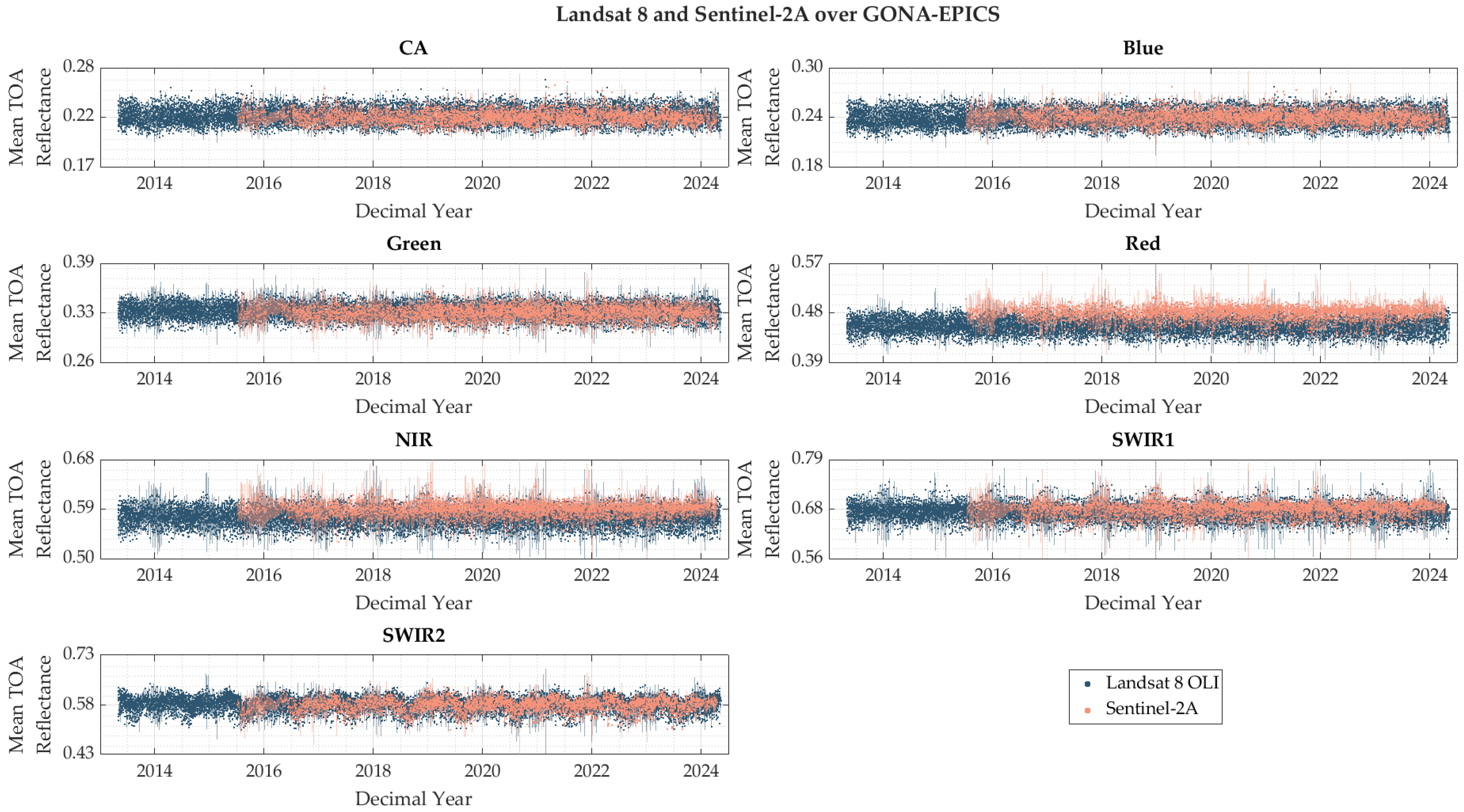
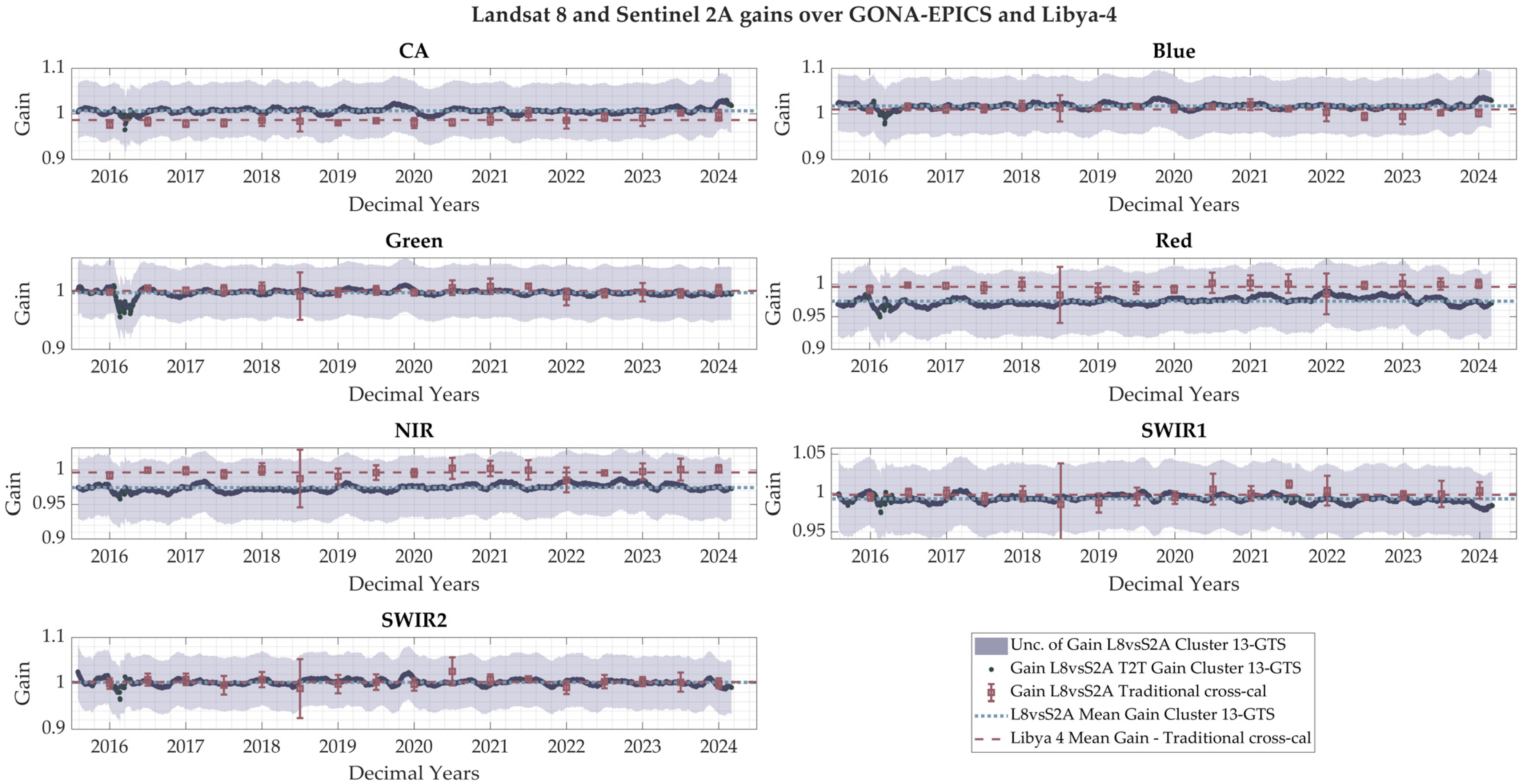
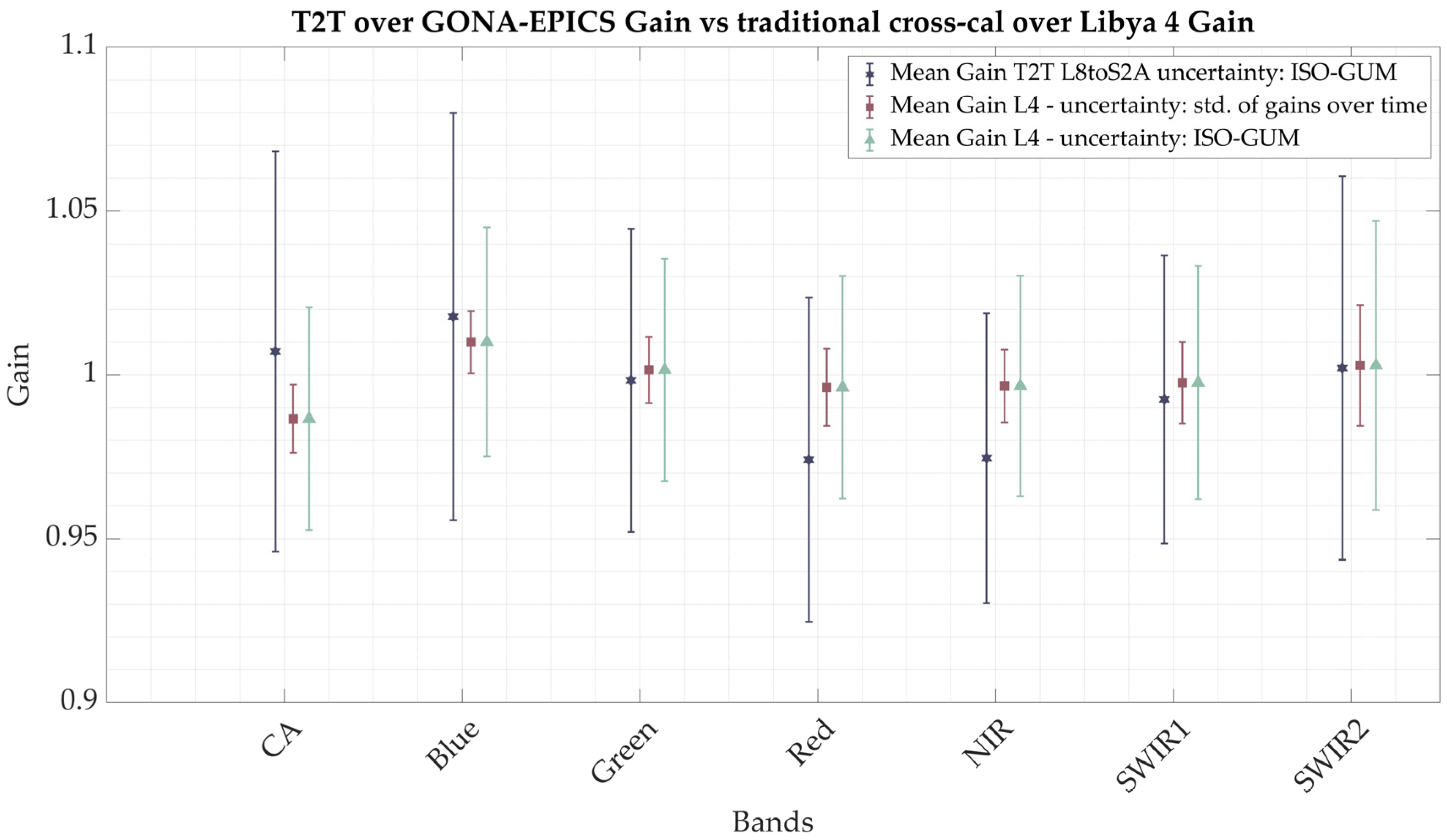
3.3.2. Results of Cross-Calibration: Traditional vs. T2T

To evaluate the applicability of the hyperspectral profiles derived in this work and the potential of EPICS identified by Fajardo et al. [16] in their cluster analysis, a cross-calibration between Landsat 8 and Sentinel-2A was conducted using Cluster 13-GTS as the calibration target. The hyperspectral profile derived in this work for that target was used to obtain the SBAF, correcting for RSR differences between the two sensors to calculate cross-calibration gain values. These results were then compared to those obtained using Libya 4 CNES ROI as the calibration target and Hyperion as the hyperspectral data source, as traditionally conducted. Cluster 13-GTS was selected for this comparison because it includes pixels from the Libya 4 CNES ROI.

Figure 18 shows the mean TOA reflectance of Cluster 13-GTS for both Landsat 8 and Sentinel-2A, used for the T2T cross-calibration. For this analysis, all locations in the IP LAB archive containing Cluster 13-GTS pixels were processed. As a result, a total of 32 tiles were used for Sentinel-2A, while 58 Path/Rows were used for Landsat 8.

Cloud filtering was performed using the quality control band provided as part of the Level 1 Collection 2 product, following the methodology detailed in Fajardo et al. [16]. Additionally, BRDF normalization was applied according to the methodology explained in Section 2.4. As described above, an MSG filter was applied to the data shown in Figure 18, and the resulting trends from this filtering are illustrated in Figure 19. In this figure, the most substantial differences are observed in the red and NIR bands. The ratio of these trends (L8/S2A) was computed to obtain a per-day gain, and the means of these gains over time represents the total gain for each band between the two sensors.

After obtaining the gains described above, a comparison was made between these gains and those derived from a more traditional cross-calibration methodology over the Libya 4 CNES ROI, as described in Section 2.8.1. This comparison is illustrated in Figure 20. In this figure, the blue data represents the gain obtained over GONA-EPICS using the T2T cross-calibration methodology, with the associated uncertainty indicated by the blue shaded area. The gains obtained through the traditional approach over the Libya 4 ROI are shown with error bars representing the average of temporal standard deviation of the gains.

As seen in the figure, the uncertainty of the GONA-EPICS encompasses the gains obtained through the traditional cross-calibration, making them statistically indistinguishable. However, the error bars for the traditional cross-calibration gains appear substantially smaller compared to the uncertainty reported for GONA-EPICS. To evaluate how the uncertainties of the traditional cross-calibration method would change if estimated using the methodology applied for GONA-EPICS following the ISO-GUM methodology, as shown in Equation (22), the sources of uncertainty for the Libya 4 CNES ROI were calculated. The total uncertainty was then computed, which included estimating SBAF uncertainty through the Monte Carlo simulation approach detailed in Section 2.7.3.

Figure 21 displays the total gain obtained for the T2T methodology, which is the mean of the gains calculated over time, alongside the gain obtained through the traditional approach, also represented as the mean of the gains over time. The uncertainties, as previously mentioned, differ and can be observed in the figure. The blue data indicates the total gain and its associated uncertainty obtained through the T2T technique, while the red and green data represent the total gain obtained through the traditional cross-calibration approach.

The error bar for the red data reflects the average of temporal standard deviations of the gains collected every six months, whereas the error bar for the green data represents the uncertainty for the traditional cross-calibration approach but calculated using the ISO-GUM methodology applied to the T2T cross-calibration, as shown in Equation (22). It is evident that the gain uncertainty may be underestimated when only the standard deviation of the gains over time is considered as the uncertainty. This approach overlooks other significant sources of uncertainty, such as SBAF uncertainty, BRDF effects, and sensor-specific uncertainties.

Furthermore, while the uncertainty of the gain obtained through the T2T technique is higher than that from the traditional Libya 4 method, following the same methodology for uncertainty calculation, the difference is less than 2.6% across all bands. The EPICS provide an uncertainty on the gain of less than 6% across all bands, compared to less than 4.4% provided by Libya 4. This indicates that the T2T cross-calibration methodology not only offers an alternative approach for cross-calibrating sensors, providing numerous calibration opportunities per cycle based on sensor cycles and orbital paths due to its global coverage, but also allows for daily calibration and monitoring, yielding statistically the same results to traditional cross-calibration methods. Additionally, this work demonstrates improvements and develops a methodology for more reliable SBAF estimation with enhanced spectral resolution, capturing the target’s signature in greater detail. This provides not only a more accurate estimate of SBAF and its uncertainty but also an improvement in the total gain uncertainty estimation. By considering all relevant sources of uncertainty—such as SBAF, BRDF effects, and sensor-specific uncertainties—this methodology enables the inclusion and proper consideration of these factors in the final gain estimate.

4. Conclusions

This work selected and derived the hyperspectral profiles of 20 EPICS, obtained from an unsupervised global land cover clustering of temporally stable pixels performed by Fajardo et al. [16]. These EPICS were chosen based on their low temporal variability through a k-means clustering algorithm, which grouped the 75 clusters from the global land cover clustering into 20 distinct groups with varying spectral characteristics. From these groups, the cluster with the smallest temporal standard deviation was selected as the EPICS. Consequently, 20 EPICS were identified, and their hyperspectral profiles were estimated using Hyperion and DESIS data.

For the hyperspectral profile generation, all available scenes in the IP LAB archive for DESIS and Hyperion sensors were used, and the validation of one of these profiles was achieved through comparison with ground truth measurements. Specifically, the mean TOA reflectance of the GONA-EPICS cluster, which contains pixels from the RadCalNet GONA site ROI, was compared to the mean TOA reflectance collected over the RadCalNet GONA site. A Welch’s test was conducted for this comparison, and the results demonstrated that the hyperspectral profile of the GONA-EPICS derived in this work is statistically indistinguishable from that derived from ground truth measurements, within their respective uncertainties.

To further validate the reliability and applicability of the hyperspectral profiles derived in this work, the SBAF between Landsat 8 and Sentinel-2A was generated through a Monte Carlo simulation using the GONA-EPICS hyperspectral profile and the profile derived from RadCalNet-GONA. This simulation accounted for the temporal variability of the hyperspectral profile for each band and the uncertainties in each sensors’ RSR. The SBAF results for the GONA-EPICS cluster and RadCalNet-GONA were statistically indistinguishable, demonstrating that the hyperspectral profiles for the 20 EPICS selected in this work yield SBAF results consistent with those obtained from ground truth measurements. Additionally, the inclusion of DESIS data reduced the SBAF uncertainty calculated using EPICS. This improvement was attributed not only to the increased number of observations but also to the enhanced spectral resolution provided by DESIS, improving from Hyperion’s 10 nm to DESIS’s 2.55 nm spectral resolution in the VNIR region.

Finally, the applicability and reliability of these EPICS and their hyperspectral profiles were demonstrated through a cross-calibration between Landsat 8 and Sentinel-2A. This was achieved using the hyperspectral profile and the SBAF methodology derived in this work, with one of the 20 selected EPICS serving as the target. For cross-calibration using EPICS, the T2T methodology was applied, and the gain obtained over Cluster 13-GTS (the EPICS target), which includes pixels from the Libya 4 traditional PICS, was compared to the gain obtained using the traditional cross-calibration methodology over the well-known Libya 4 CNES ROI. The gain results from both targets and methodologies were statistically similar, with EPICS uncertainty better than 6% across all bands, compared to 4.4% for the traditional cross-calibration methodology. Additionally, these EPICS provide the advantage of enabling daily cross-calibration analysis between the two sensors under study due to their global coverage, in contrast to the limited observations provided by traditional PICS (

Table 1. Total Gain obtained using Cluster 13-GTS and Libya 4. The table includes uncertainty values calculated using the traditional method and those calculated following the ISO-GUM methodology for Libya 4.

	CA	Blue	Green	Red	NIR	SWIR1	SWIR2
Gain T2T	1.01	1.02	1	0.97	0.97	0.99	1
Unc. T2T (%)	6.08	6.07	4.61	5.1	4.54	4.4	5.71
Gain L4	0.98	1.01	0.99	0.99	0.99	0.99	1
Std. L4 (%)	1.04	0.95	1.01	1.17	1.11	1.24	1.84
Gain L4	0.98	1.01	0.99	0.99	0.99	0.99	1
Unc. L4 (%)	3.45	3.46	3.39	3.41	3.38	3.57	4.4

).

This analysis also highlighted that gain uncertainty may be underestimated when only the temporal variability of the site is considered, as is traditionally conducted. Other sources of uncertainty—including SBAF uncertainty, BRDF uncertainty, and the reference sensor’s absolute uncertainty—should also be included in uncertainty calculations. The methodology presented in this work incorporates these sources, offering a more comprehensive and accurate uncertainty estimation.

The outcome of this work provides the scientific community with a set of targets suitable for radiometric calibration and stability monitoring, offering daily cross-calibration opportunities for any sensor in any orbital path due to their global coverage. These targets also support calibration and stability monitoring for sensors with varying spatial resolutions, as EPICS are composed of aggregated pixels with similar spectral characteristics that span vast regions and are globally distributed. These unique characteristics make them suitable for both high and coarse spatial resolution sensors. This can be an advantage for the calibration of future hyperspectral missions such as SI-Traceable Satellites (SITSats) like CLARREO-Pathfinder and other future missions. One limitation of these space-based methods is their operational necessity to maintain consistent geometric positioning relative to the satellite being calibrated. This requirement often results in a limited number of coincident data collections. While these collections provide a robust anchoring for calibration, the quantity of observations and the flexibility in timing and location are constrained. The targets presented in this work could complement these space-based efforts by bridging the temporal gaps left by the limited coincident collections of SITSats. By leveraging EPICS, which can gather data more frequently and flexibly than any traditional PICS or RadCalNet sites, a more continuous calibration timeline is possible. This allows for an increased number of cross-calibration opportunities, enhancing the robustness and reliability of the calibration over time.

This study not only provides potential EPICS as global calibration targets but also introduces EPICS with a wider spectral range with defined uncertainties, enabling their use for calibration across different reflectance levels, in contrast to traditional methodologies. Additionally, this work presents, for the first time, the derivation of hyperspectral profiles assigned to the global EPICS. These profiles facilitate more efficient sensor calibration and monitoring on a global scale, offering improved spectral resolution and capturing finer details crucial for future missions with a focus on hyperspectral capabilities.

Future work may build upon the methodology presented in this study to derive hyperspectral profiles for additional targets and enhance the existing profiles by integrating new hyperspectral data sources with improved spectral resolution and reduced uncertainties, such as those expected from missions like the ones mentioned above. In addition, given that the total uncertainty of EPICS hyperspectral profiles includes the sensors’ absolute uncertainties, the introduction of missions with lower uncertainties could further reduce the final uncertainty of these profiles. However, while these advancements are anticipated, the profiles and sensors from which hyperspectral data were collected in this study currently meet the need for hyperspectral information until other sensors with advanced technologies become available.

References

1. Zhang, X.; Friedl, M.A.; Schaaf, C.B.; Strahler, A.H.; Hodges, J.C.; Gao, F.; Reed, B.C.; Huete, A. Monitoring vegetation phenology using MODIS. Remote Sens. Environ. 2003, 84, 471–475. [Google Scholar] [CrossRef]
2. Wiedinmyer, C.; Quayle, B.; Geron, C.; Belote, A.; McKenzie, D.; Zhang, X.; O’Neill, S.; Wynne, K.K. Estimating emissions from fires in North America for air quality modeling. Atmos. Environ. 2006, 40, 3419–3432. [Google Scholar] [CrossRef]
3. Youssef, A.; Pradhan, B.; Tarabees, E. Integrated evaluation of urban development suitability based on remote sensing and GIS techniques: Contribution from the analytic hierarchy process. Arab. J. Geosci. 2011, 4, 463–473. [Google Scholar] [CrossRef]
4. Aiken, J.; Moore, G.F.; Hotligan, P.M. Remote sensing of oceanic biology in relation to global climate change. J. Phycol. 1992, 28, 579–590. [Google Scholar] [CrossRef]
5. Czapla-Myers, J.; McCorkel, J.; Anderson, N.; Thome, K.; Biggar, S.; Helder, D.; Aaron, D.; Leigh, L.; Mishra, N. The ground-based absolute radiometric calibration of Landsat 8 OLI. Remote Sens. 2015, 7, 600–626. [Google Scholar] [CrossRef]
6. Wyatt, C. Radiometric Calibration: Theory and Methods; Elsevier: Amsterdam, The Netherlands, 2012. [Google Scholar]
7. Helder, D.L.; Karki, S.; Bhatt, R.; Micijevic, E.; Aaron, D.; Jasinski, B. Radiometric calibration of the Landsat MSS sensor series. IEEE Trans. Geosci. Remote Sens. 2011, 50, 2380–2399. [Google Scholar] [CrossRef]
8. Xiong, X.; Barnes, W. An overview of MODIS radiometric calibration and characterization. Adv. Atmos. Sci. 2006, 23, 69–79. [Google Scholar] [CrossRef]
9. Chander, G.; Meyer, D.J.; Helder, D.L. Cross calibration of the Landsat-7 ETM+ and EO-1 ALI sensor. IEEE Trans. Geosci. Remote Sens. 2004, 42, 2821–2831. [Google Scholar] [CrossRef]
10. Teillet, P.; Barker, J.; Markham, B.; Irish, R.; Fedosejevs, G.; Storey, J. Radiometric cross-calibration of the Landsat-7 ETM+ and Landsat-5 TM sensors based on tandem data sets. Remote Sens. Environ. 2001, 78, 39–54. [Google Scholar] [CrossRef]
11. Lacherade, S.; Fougnie, B.; Henry, P.; Gamet, P. Cross calibration over desert sites: Description, methodology, and operational implementation. IEEE Trans. Geosci. Remote Sens. 2013, 51, 1098–1113. [Google Scholar] [CrossRef]
12. Barsi, J.A.; Alhammoud, B.; Czapla-Myers, J.; Gascon, F.; Haque, M.O.; Kaewmanee, M.; Leigh, L.; Markham, B.L. Sentinel-2A MSI and Landsat-8 OLI radiometric cross comparison over desert sites. Eur. J. Remote Sens. 2018, 51, 822–837. [Google Scholar] [CrossRef]
13. Angal, A.; Mishra, N.; Xiong, X.; Helder, D. Cross-calibration of Landsat 5 TM, and Landsat 8 OLI with Aqua MODIS using PICS. In Proceedings of the Earth Observing Systems XIX, San Diego, CA, USA, 18–20 August 2014; pp. 171–179. [Google Scholar]
14. Mishra, N.; Haque, M.O.; Leigh, L.; Aaron, D.; Helder, D.; Markham, B. Radiometric cross calibration of Landsat 8 operational land imager (OLI) and Landsat 7 enhanced thematic mapper plus (ETM+). Remote Sens. 2014, 6, 12619–12638. [Google Scholar] [CrossRef]
15. Fajardo Rueda, J.; Leigh, L.; Teixeira Pinto, C.; Kaewmanee, M.; Helder, D. Classification and Evaluation of Extended PICS (EPICS) on a Global Scale for Calibration and Stability Monitoring of Optical Satellite Sensors. Remote Sens. 2021, 13, 3350. [Google Scholar] [CrossRef]
16. Fajardo Rueda, J.; Leigh, L.; Teixeira Pinto, C. Identification of Global Extended Pseudo Invariant Calibration Sites (EPICS) and Their Validation Using Radiometric Calibration Network (RadCalNet). Remote Sens. 2024, 16, 4129. [Google Scholar] [CrossRef]
17. Khakurel, P.; Leigh, L.; Kaewmanee, M.; Pinto, C.T. Extended pseudo invariant calibration site-based trend-to-trend cross-calibration of optical satellite sensors. Remote Sens. 2021, 13, 1545. [Google Scholar] [CrossRef]
18. Shah, R.; Leigh, L.; Kaewmanee, M.; Pinto, C.T. Validation of Expanded Trend-to-Trend Cross-Calibration Technique and Its Application to Global Scale. Remote Sens. 2022, 14, 6216. [Google Scholar] [CrossRef]
19. Rengarajan, R.; Schott, J.R. Evaluation of sensor and environmental factors impacting the use of multiple sensor data for time-series applications. Remote Sens. 2018, 10, 1678. [Google Scholar] [CrossRef]
20. Folkman, M.A.; Pearlman, J.; Liao, L.B.; Jarecke, P.J. EO-1/Hyperion hyperspectral imager design, development, characterization, and calibration. Hyperspectral Remote Sens. Land Atmos. 2001, 4151, 40–51. [Google Scholar]
21. Krutz, D.; Müller, R.; Knodt, U.; Günther, B.; Walter, I.; Sebastian, I.; Säuberlich, T.; Reulke, R.; Carmona, E.; Eckardt, A. The instrument design of the DLR earth sensing imaging spectrometer (DESIS). Sensors 2019, 19, 1622. [Google Scholar] [CrossRef] [PubMed]
22. Chaity, M.D.; Kaewmanee, M.; Leigh, L.; Teixeira Pinto, C. Hyperspectral Empirical Absolute Calibration Model Using Libya 4 Pseudo Invariant Calibration Site. Remote Sens. 2021, 13, 1538. [Google Scholar] [CrossRef]
23. Karki, P.B.; Kaewmanee, M.; Leigh, L.; Pinto, C.T. The Development of Dark Hyperspectral Absolute Calibration Model Using Extended Pseudo Invariant Calibration Sites at a Global Scale: Dark EPICS-Global. Remote Sens. 2023, 15, 2141. [Google Scholar] [CrossRef]
24. Fajardo Rueda, J.; Leigh, L.; Pinto, C.T. A Global Mosaic of Temporally Stable Pixels for Radiometric Calibration of Optical Satellite Sensors Using Landsat 8. Remote Sens. 2024, 16, 2437. [Google Scholar] [CrossRef]
25. Ungar, S.G.; Pearlman, J.S.; Mendenhall, J.A.; Reuter, D. Overview of the earth observing one (EO-1) mission. IEEE Trans. Geosci. Remote Sens. 2003, 41, 1149–1159. [Google Scholar] [CrossRef]
26. Franks, S.; Neigh, C.S.; Campbell, P.K.; Sun, G.; Yao, T.; Zhang, Q.; Huemmrich, K.F.; Middleton, E.M.; Ungar, S.G.; Frye, S.W. EO-1 data quality and sensor stability with changing orbital precession at the end of a 16 year mission. Remote Sens. 2017, 9, 412. [Google Scholar] [CrossRef]
27. Shrestha, M.; Sampath, A.; Chandra, S.N.R.; Christopherson, J.; Shaw, J.; Anderson, C. System Characterization Report on the German Aerospace Center (DLR) Earth Sensing Imaging Spectrometer (DESIS); US Geological Survey: Reston, VA, USA, 2021; ISSN 2331-1258. [Google Scholar]
28. Frank Warmerdam, E.R. GDAL Documentation. Available online: http://www.gdal.org/ (accessed on 5 March 2024).
29. Alonso, K.; Bachmann, M.; Burch, K.; Carmona, E.; Cerra, D.; De los Reyes, R.; Dietrich, D.; Heiden, U.; Hölderlin, A.; Ickes, J. Data products, quality and validation of the DLR earth sensing imaging spectrometer (DESIS). Sensors 2019, 19, 4471. [Google Scholar] [CrossRef] [PubMed]
30. Monali Adrija, H.; Larry, L.; Kaewmanee, M.; Rueda, J.F.; Pathiranage, D.S.; Pinto, C.T. Absolute Vicarious Calibration, Extended PICS (EPICS) based De-trending and Validation of Hyperspectral Hyperion, DESIS, and EMIT. 2025; unpublished. [Google Scholar]
31. Biggar, S.F.; Thome, K.J.; Wisniewski, W. Vicarious radiometric calibration of EO-1 sensors by reference to high-reflectance ground targets. IEEE Trans. Geosci. Remote Sens. 2003, 41, 1174–1179. [Google Scholar] [CrossRef]
32. Jing, X.; Leigh, L.; Helder, D.; Pinto, C.T.; Aaron, D. Lifetime absolute calibration of the EO-1 Hyperion sensor and its validation. IEEE Trans. Geosci. Remote Sens. 2019, 57, 9466–9475. [Google Scholar] [CrossRef]
33. Farhad, M.M.; Kaewmanee, M.; Leigh, L.; Helder, D. Radiometric cross calibration and validation using 4 angle BRDF model between landsat 8 and sentinel 2A. Remote Sens. 2020, 12, 806. [Google Scholar] [CrossRef]
34. Shrestha, M. Bidirectional Reflectance Distribution Function of Algodones Dunes. Master’s Thesis, South Dakota State University, Brookings, SD, USA, 2016. [Google Scholar]
35. Kaewmanee, M. Pseudo invariant calibration sites: PICS evolution. In Proceedings of the CALCON 2018, Logan, UT, USA, 18–20 June 2018. [Google Scholar]
36. McCorkel, J.; Thome, K.; Ong, L. Vicarious calibration of EO-1 Hyperion. IEEE J. Sel. Top. Appl. Earth Observ. Remote Sens. 2012, 6, 400–407. [Google Scholar] [CrossRef]
37. Bouvet, M.; Thome, K.; Berthelot, B.; Bialek, A.; Czapla-Myers, J.; Fox, N.P.; Goryl, P.; Henry, P.; Ma, L.; Marcq, S. RadCalNet: A radiometric calibration network for Earth observing imagers operating in the visible to shortwave infrared spectral range. Remote Sens. 2019, 11, 2401. [Google Scholar] [CrossRef]
38. Marcq, S.; Meygret, A.; Bouvet, M.; Fox, N.; Greenwell, C.; Scott, B.; Berthelot, B.; Besson, B.; Guilleminot, N.; Damiri, B. New RadCalNet site at Gobabeb, Namibia: Installation of the instrumentation and first satellite calibration results. In Proceedings of the IGARSS 2018—2018 IEEE International Geoscience and Remote Sensing Symposium, Valencia, Spain, 22–27 July 2018; pp. 6444–6447. [Google Scholar]
39. RadCalNet. RadCalNet Quick Start Guide. Available online: https://www.radcalnet.org (accessed on 18 June 2024).
40. Lu, Z.; Yuan, K.-H. Welch’st test. Encycl. Res. Des. 2010, 1, 1620–1623. [Google Scholar]
41. Revel, C.; Lonjou, V.; Marcq, S.; Desjardins, C.; Fougnie, B.; Coppolani-Delle Luche, C.; Guilleminot, N.; Lacamp, A.-S.; Lourme, E.; Miquel, C. Sentinel-2A and 2B absolute calibration monitoring. Eur. J. Remote Sens. 2019, 52, 122–137. [Google Scholar] [CrossRef]
42. Gascon, F.; Bouzinac, C.; Thépaut, O.; Jung, M.; Francesconi, B.; Louis, J.; Lonjou, V.; Lafrance, B.; Massera, S.; Gaudel-Vacaresse, A. Copernicus Sentinel-2A calibration and products validation status. Remote Sens. 2017, 9, 584. [Google Scholar] [CrossRef]
43. Pinto, C.T.; Ponzoni, F.J.; Castro, R.M.; Leigh, L.; Kaewmanee, M.; Aaron, D.; Helder, D. Evaluation of the uncertainty in the spectral band adjustment factor (SBAF) for cross-calibration using Monte Carlo simulation. Remote Sens. Lett. 2016, 7, 837–846. [Google Scholar] [CrossRef]
44. Berthelot, B.; Meygret, A.; Desjardins, C. Monitoring the Intercalibration of L8/OLI with S2A/MSI over Libya4 PICS in the Frame of PICSCAR CEOS/IVOS Initiative. 2021. Available online: https://az659834.vo.msecnd.net/eventsairwesteuprod/production-nikal-public/27b62454333f4236a59b7574911d76d8 (accessed on 18 June 2024).
45. Pinto, C.T.; Shrestha, M.; Hasan, N.; Leigh, L.; Helder, D. SBAF for cross-calibration of Landsat-8 OLI and Sentinel-2 MSI over North African PICS. In Proceedings of the Earth Observing Systems XXIII, San Diego, CA, USA, 21–23 August 2018; pp. 294–304. [Google Scholar]
Figure 1. Inventory of all scenes available in IP LAB archive for DESIS (yellow) and Hyperion (green).
Remotesensing 17 00216 g001
Figure 2. Pixel distribution of Cluster 69 across North Africa. Green data represents pixels extracted in mask for latitude 028, longitude 023.
Remotesensing 17 00216 g002
Figure 3. Atmospheric transmittance and band selection for cloud mask derivation for DESIS and Hyperion.
Remotesensing 17 00216 g003
Figure 4. An example of the dynamic 3-sigma outlier rejection threshold. The shaded area indicates the threshold.
Remotesensing 17 00216 g004
Figure 5. Example of spectral interpolation of Hyperion data to match DESIS 2.55 nm for 400 nm to 1000 nm range.
Remotesensing 17 00216 g005
Figure 6. An example of the data used for the hyperspectral profile generation of Cluster 72 (top chart) and the resulting hyperspectral profile for Cluster 72 (bottom chart).
Remotesensing 17 00216 g006
Figure 7. Pixel distribution of GONA-EPICS on global scale, shown in magenta. Blue squares represent DESIS locations utilized, while green stars indicate Hyperion locations used.
Remotesensing 17 00216 g007
Figure 8. A flow chart of the methodology used to perform the Monte Carlo simulation to obtain the SBAF and its uncertainty.
Remotesensing 17 00216 g008
Figure 9. The top chart shows the Landsat 8 RSR along with its uncertainty. The middle chart displays the Sentinel-2 RSR and its uncertainty, while the bottom chart presents the hyperspectral profile derived using DESIS and Hyperion data.
Remotesensing 17 00216 g009
Figure 10. An example of the k-means results for the 20 groups. The charts on the left display the clusters aggregated in each group, while the charts on the right show the selected EPICS for each group based on their temporal standard deviation.
Remotesensing 17 00216 g010
Figure 11. EPICS selected through k-means clustering algorithm.
Remotesensing 17 00216 g011
Figure 12. The pixel distribution of the 20 EPICS selected in this work. Each color represents the pixels belonging to a specific EPICS. For example, cyan indicates Cluster 55, while yellow represents Cluster 128.
Remotesensing 17 00216 g012
Figure 13. Scene count for derivation of hyperspectral profiles for each cluster: DESIS (left) and Hyperion (right).
Remotesensing 17 00216 g013
Figure 14. Hyperspectral profiles derived in this work using DESIS and Hyperion data for 20 EPICS selected.
Remotesensing 17 00216 g014
Figure 15. Validation of mean TOA reflectance of GONA-EPICS versus RadCalNet. Uncertainties of both datasets are represented as shaded areas.
Remotesensing 17 00216 g015
Figure 16. The top chart displays the mean TOA reflectance of GONA-EPICS and RadCalNet GONA, with the corresponding uncertainties represented as shaded areas, used as inputs for Welch’s test. The bottom chart presents the p-values resulting from this test, with a horizontal line indicating the significance level of 0.05.
Remotesensing 17 00216 g016
Figure 17. The SBAF results obtained from the hyperspectral profiles in this study. The SBAF derived from the hyperspectral profile using Hyperion data over GONA-EPICS is shown in light green. The SBAF derived from the hyperspectral profile using both DESIS and Hyperion data over GONA-EPICS is represented in blue. The SBAF derived from RadCalNet-GONA data is indicated in brown.
Remotesensing 17 00216 g017
Figure 18. BRDF-normalized mean TOA reflectance of Landsat 8 and Sentinel-2A over GONA-EPICS.
Remotesensing 17 00216 g018
Figure 19. Trends obtained for Landsat 8 and Sentinel-2A data over GONA-EPICS.
Remotesensing 17 00216 g019
Figure 20. Comparison of gain (L8/S2A) obtained through T2T cross-calibration approach versus traditional cross-calibration gain over Libya 4.
Remotesensing 17 00216 g020
Figure 21. Gain obtained using T2T cross-calibration (blue) with error bars computed using ISO-GUM. Gain obtained through traditional approach (brown) with error bars calculated as temporal standard deviation. Gain obtained through traditional method (light green) with error bars computed using ISO-GUM.
Remotesensing 17 00216 g021