Highlights
What are the main findings?
- Developed 3DV-Unet, an end-to-end deep learning framework that reconstructs eddy-resolving three-dimensional (3D) essential ocean variables (temperature, salinity, and zonal/meridional velocities) from multi-source satellite observations.
- Demonstrated high-resolution 3D reconstructions with RMSEs of ~0.30 °C (temperature), 0.11 psu (salinity), and ~0.05 m/s (currents), all with R2 > 0.93. Comprehensive error and spectral analyses reveal good agreement at the 100-km scale, though systematic deviations occur in dynamically complex regions (e.g., Kuroshio Extension) and within the 20–100 km band.
What is the implication of the main finding?
- The reconstructed 3D fields can reproduce mesoscale eddy structures and their life cycle and evolution, enabling detailed investigation of ocean dynamics.
- The high-resolution EOV reconstructions generated by 3DV-Unet provide a valuable resource for physical oceanography and climate studies, supporting analyses of energy transport, mixing processes, and regional variability.
Abstract
Three-dimensional (3D) ocean physical fields are essential for understanding ocean dynamics, but reconstructing them solely from sea-surface remote sensing remains challenging. We present 3DV-Unet, an end-to-end deep learning framework that reconstructs eddy-resolving three-dimensional essential ocean variables (temperature, salinity, and currents) from multi-source satellite data. The model employs a 3D Vision Transformer bottleneck to capture cross-depth and cross-variable dependencies, ensuring physically consistent reconstruction. Trained on 2011–2019 reanalysis and satellite data, 3DV-Unet achieves RMSEs of ~0.30 °C for temperature, 0.11 psu for salinity, and 0.05 m/s for currents, with all R2 values above 0.93. Error analyses further indicate higher reconstruction errors in dynamically complex regions such as the Kuroshio Extension, while spectral analysis indicates good agreement at 100 km+ but systematic deviation in the 20–100 km band. Independent validation against 6113 Argo profiles confirms its ability to reproduce realistic vertical thermohaline structures. Moreover, the reconstructed 3D fields capture mesoscale eddy structures and their life cycle, offering a valuable basis for investigating ocean circulation, energy transport, and regional variability. These results demonstrate the potential of end-to-end volumetric deep learning for advancing high-resolution 3D ocean reconstruction and supporting physical oceanography and climate studies.
1. Introduction
Ocean temperature, salinity, and current velocity are essential variables characterizing marine dynamical systems, ecosystems, and climate [1,2,3,4]. Modeling the 3D fields of these variables is indispensable for investigating critical topics such as marine heatwaves [4,5], ocean stratification [6], El Niño–Southern Oscillation (ENSO) [7,8], and global energy and material transport [9,10].
However, acquiring subsurface ocean data remains a formidable challenge. In situ platforms such as Argo floats, moorings, and ship-based measurements provide accurate subsurface observations, but their coverage is still limited compared to the vast global ocean, and existing profiles are insufficient to fully resolve the multi-scale structures of the ocean interior [11,12,13,14]. Consequently, developing robust methods for reconstructing 3D ocean physical fields from limited observations is essential [6,15,16].
Compared with in situ observations, satellite data offer high temporal–spatial resolution and broad coverage but are mainly restricted to surface or near-surface variables (e.g., SLA, SST, SSS), which cannot directly provide information about the ocean interior. Studies have shown that subsurface properties can be inferred from them [17,18,19]. Therefore, leveraging the physical linkages between the surface and subsurface ocean to reconstruct 3D subsurface physical fields from satellite observations has emerged as a viable technical pathway.
To reconstruct 3D ocean fields, methods can be grouped into four types: (i) physics-driven, (ii) empirical statistical, (iii) machine learning, and (iv) deep learning [20]. Physics-driven methods use local physical conditions but struggle to generalize in the ocean’s complex environment [21,22,23,24]. Empirical statistical methods link surface and subsurface variables through linear or weakly nonlinear relationships and are widely used for temperature and salinity reconstruction [25,26,27], but their performance drops in data-sparse regions [28]. Machine learning methods model more complex nonlinear relationships, paving the way for advanced deep learning approaches [29,30,31].
In recent years, deep learning has advanced 3D ocean reconstruction in three main aspects: (i) model architectures, (ii) spatial resolution, and (iii) output dimensionality.
Convolutional Neural Networks (CNN) have long served as the backbone for their strong spatial feature extraction [32]. With the rise of Transformers, Vision Transformer (ViT) employs global self-attention over patch tokens, whereas Swin Transformer introduces window-based hierarchical attention with shifted windows and patch merging for multi-scale representations [33,34,35]. U-Net remains widely used for regional reconstruction due to its ability to integrate multi-scale features and preserve fine details [36].
Training data resolution strongly affects reconstruction capability. Low resolution labels (e.g., 1°) mainly capture large-scale circulation, while medium-resolution products like ARMOR3D (1/4°) resolve mesoscale variability [37,38,39,40,41,42]. High-resolution reanalysis datasets such as HYCOM and GLORYS12 (1/12°) partially represent submesoscale signatures but demand greater model capacity and computational resources [43,44,45,46,47].
Model outputs have evolved from single-point vertical profiles [48,49,50] to 2D horizontal slices [46,51,52,53], and now to full 3D volumetric reconstruction. Existing approaches, however, often emphasize either single-variable fields at high resolution or multi-variable reconstructions at lower resolution, which may fail to capture submesoscale and other fine-scale variability [42,45,54]. The 3D ocean physical field is a highly coupled system with complex nonlinear dependencies among different variables, across depth levels, and between horizontal locations. Current model architectures still face challenges in explicitly representing these comprehensive “3D plus multi-variable” correlations, which remain a frontier issue in the field [51,52,53,54]. To address this gap, we propose 3DV-Unet, a high-resolution, multi-variable reconstruction model centered on a 3D Vision Transformer (ViT-3D) with dual attention: one path captures horizontal interactions, and the other captures vertical dependencies and inter-variable relationships such as temperature–salinity coupling. This design enables explicit and efficient modeling of the coupled “3D + multi-variable” correlations in complex ocean systems.
The paper is structured as follows: Section 2 describes the study area, datasets, and preprocessing; Section 3 details the 3DV-Unet architecture—especially the ViT-3D core; Section 4 reports results, including baseline comparisons, spatiotemporal analysis, and Argo validation; Section 5 discusses the findings; Section 6 concludes and outlines future work.
2. Study Area and Data
2.1. Study Area
The study area is the Northwest Pacific Ocean and the South China Sea (0°N–60°N, 100°E–160°E), encompassing marginal seas, open ocean, and narrow straits. The area encompasses semi-enclosed marginal seas, eddy-active zones, and an energetic western-boundary current region, producing pronounced mixed-layer and thermocline variability within the upper 0–500 m. This diversity forms a stringent testbed for end-to-end 3D reconstruction, allowing us to evaluate model performance in different environments and to probe the generalization–specialization balance of the pretrain–fine-tune strategy.
To isolate and compare the effects of these distinct regional factors, the study area was strategically partitioned into four 20° × 20° sub-regions (Figure 1). This partitioning framework allows for a multifaceted comparison addressing the following objectives:
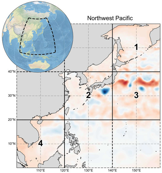
Figure 1.
The study area in this work is the Northwest Pacific (100°E–160°E, 0°N–60°N), which has been partitioned into the four sub-regions that are marked by solid lines in the figure (Sub-regions 1–4). The background displays the Sea Level Anomaly (SLA) field for 1 January 2016.
- Ensuring adequate coverage and representativeness of the dataset for training and evaluation;
- An investigation into the coupling between model performance and geographic location, which assesses the feasibility of developing a generalized regional reconstruction model;
- Evaluating the generalization capability of a unified model when it is applied to the distinct oceanographic regimes of each sub-region;
- An analysis of the impact of specific dominant factors (e.g., western boundary currents, coastal processes) on the model’s reconstruction accuracy.
Specifically, the spatial extents and main oceanographic characteristics of the four sub-regions are as follows:
- Sub-region 1 (40–60°N, 140–160°E): the Sea of Okhotsk, a semi-enclosed marginal sea with broad shelves and relatively low eddy kinetic energy (EKE).
- Sub-region 2 (20–40°N, 120–140°E): the upstream Kuroshio and adjacent shelf seas, influenced by monsoon forcing and exhibiting moderate eddy activity.
- Sub-region 3 (20–40°N, 140–160°E): the Kuroshio Extension, an energetic western boundary current system with strong fronts, meanders, and the highest EKE among the four regions.
- Sub-region 4 (0–20°N, 100–120°E): the South China Sea, where complex bathymetry, monsoon forcing, and strait exchanges produce highly variable circulation.
2.2. Data
This study utilizes a comprehensive suite of multi-source satellite remote sensing products, reanalysis data, and in situ observations to construct and evaluate the 3D ocean reconstruction model. The input variables were specifically selected to enable the reconstruction of three-dimensional ocean physical fields from satellite observations, all of which can be derived from satellite-based products and directly influence the evolution of temperature, salinity, and ocean circulation. Each dataset was therefore chosen for both its high quality and its direct physical relevance to the oceanic processes being modeled. A summary of all datasets used in this study is provided in Table 1, detailing the data types, temporal coverage, spatial resolution, variables, and sources.

Table 1.
Information on data products and sources used in this study. All data sources were accessed on 1 August 2025.
2.2.1. Remote Sensing Data
Surface inputs comprised Sea Level Anomaly (SLA) and absolute geostrophic currents (UGOS/VGOS) from the CMEMS Global Ocean Gridded L4 Sea Surface Heights and Derived Variables (reprocessed); Sea Surface Salinity (SSS) from the CMEMS Multi-Observation SSS/SSD product; Sea Surface Temperature (SST) from GHRSST L4 REMSS MW_IR_OI_GLOB v2.0; 10 m winds (UWND/VWND) from CCMP v3.1; and precipitation from the Global Multi-source Merging-and-Calibration Precipitation (GMCP) dataset.
2.2.2. Reanalysis Data
We use the 3D temperature, salinity, and horizontal current (U, V) fields from the CMEMS GLORYS12v1 “Global Ocean Physics Reanalysis” product as the ground truth data for model training. This dataset provides daily global data at a high spatial resolution of 1/12° grid.
2.2.3. In Situ Data
To independently validate our model, we use Argo temperature and salinity profile data for comparison with the model outputs. Profiles located within the Northwest Pacific region during 2011–2019 are first selected, and only those with an optimal quality control flag for the entire profile are retained. Each retained profile is then matched to the nearest model grid point within a 4 km radius and the closest available time step using a nearest-neighbor search algorithm, ensuring spatial–temporal consistency between observations and model data.
2.2.4. Ancillary Data
This study uses the ETOPO 2022v1 global relief model to generate a land–sea mask for the input data, to ensure that only oceanic grid cells are considered in the calculations.
2.3. Data Preprocessing
To prepare the datasets listed in Table 1 for model training and evaluation, a series of preprocessing steps was systematically performed. The data processing is described below:
- All datasets were interpolated to a daily temporal resolution and a spatial resolution of 1/12° using bilinear interpolation, consistent with GLORYS12.
- All input and output data are processed using sea–land masking to ensure that model errors are calculated only on valid ocean data, thereby ensuring fair and consistent evaluation.
- All input and label data have undergone min–max normalization, scaling their values to a uniform range of [0, 1] to ensure stability in model training and consistency in result evaluation.
3. Methods
3.1. Overall Architecture
To reconstruct 3D ocean physical fields from multi-source 2D sea surface observations, we propose the 3DV-Unet (Figure 2), which integrates Convolutional Neural Networks (CNNs), Vision Transformers (ViTs), and a U-Net backbone. CNN modules capture local spatial features and fine-scale patterns, as demonstrated to be effective in previous subsurface reconstructions [53,55]. The ViT component introduces self-attention to model long-range dependencies and global relationships, which has been emphasized in recent Transformer-based approaches [46]. The U-Net structure, with its encoder–decoder design and skip connections, enables multi-scale feature fusion and accurate volumetric restoration, and has been widely applied in thermohaline and eddy reconstructions [13,41,50]. By combining these complementary modules, the 3DV-Unet balances local detail preservation and global contextual understanding, consistent with recent advances in hybrid CNN–Transformer architectures for oceanographic applications.
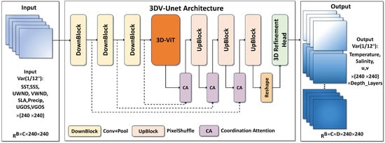
Figure 2.
Architecture of the proposed 3DV-Unet model. The network takes multi-source 2D surface variables as input, processes them through an encoder, ViT-3D block, and decoder with Coordinate Attention (CA), and outputs high-resolution 3D reconstructions of temperature, salinity, and velocity fields.
3.1.1. Input Layer
The model is fed with daily averaged 2D sea surface variable fields with a spatial resolution of 1/12°. The input data comprises eight physical quantities: Sea Surface Temperature (SST), Sea Surface Salinity (SSS), Sea Level Anomaly (SLA), Precipitation (Precip), Geostrophic Currents (UGOS, VGOS), zonal and meridional 10 m winds (UWND, VWND).
3.1.2. Encoder
As shown in Figure 2, the input data is first processed by a CNN encoder composed of three cascaded down-sampling blocks (DownBlock). Each DownBlock, containing convolution (Conv) and pooling (Pool) operations, is responsible for hierarchically extracting multi-scale spatial features from the input 2D feature maps.
3.1.3. Bottleneck
The network’s bottleneck features the ViT-3D module, which transforms 2D feature maps into a latent space capable of representing 3D structural information. Leveraging the self-attention mechanism of Transformers, it effectively captures long-range dependencies and builds physical connections between surface observations and subsurface structures—an ability that conventional CNNs lack. This is the core design of the model, with details presented in Section 3.2.
3.1.4. Skip Connections with Coordinate Attention
To ensure that high-resolution spatial details captured in the shallow layers of the encoder are faithfully transmitted to the decoder, the model employs classical skip connections. This design is crucial for preventing gradient vanishing and for recovering fine-grained structures. Notably, we integrate a CA module into the skip connection pathways. The CA module introduces a spatially aware adaptive weighting mechanism prior to feature fusion. By explicitly modeling and leveraging the spatial coordinate information of the features, it enables the network to differentiate the importance of features at various locations. Consequently, it selectively enhances crucial feature signals that contribute significantly to the 3D reconstruction task (e.g., gradients associated with ocean fronts and eddies) while effectively suppressing background or redundant information. This transition from simple concatenation to weighted fusion facilitates more efficient and precise cross-level feature utilization, ultimately leading to a significant improvement in the model’s capability for the representation and restoration of fine ocean structures.
3.1.5. Decoder
The decoder section adopts a symmetric U-Net structure, consisting of three up-sampling blocks (UpBlock), as illustrated in Figure 2. It progressively restores the spatial resolution of the feature maps through sub-pixel convolution upsampling (PixelShuffle) operations to reconstruct the 3D structure [56].
3.1.6. Output Layer
Following the decoder and reshape, features are fed to a 3D Refinement Head implemented as five stacked 3D convolutional layers. This head applies final correction and smoothing in the native 3D (x–y–z) space to enhance physical coherence across depths and variables. The model then outputs high-resolution 3D fields—temperature, salinity, and the zonal (u) and meridional (v) velocity components.
3.2. Core Bottleneck Module
A core challenge in inferring 3D ocean structures from 2D sea surface data is to effectively model the complex variations in physical quantities. To overcome this limitation, we designed the ViT-3D module as the model’s bottleneck. It is important to note that while we term it a ViT-3D module for its function of processing 3D information, our core bottleneck does not rely on 3D convolutions. Instead, it ingeniously embeds spatial depth and variable information into the channel dimension of 2D feature maps and subsequently applies channel and spatial attention mechanisms alternately. This design facilitates the interaction of information across different spatial locations, depth levels, and variables, thereby capturing contextual dependencies in both the 3D spatial and variable domains. The architecture of the ViT-3D module is illustrated in Figure 3, which consists of the following three main components:

Figure 3.
Architecture of the ViT-3D Module, consisting of depth extension, patch encoding, 3D Transformer processing, and multi-stage attention modeling.
3.2.1. Depth-Aware Positional Encoding and Feature Initialization
The primary objective of this stage is to elevate the 2D features into an initial 3D feature volume, wherein the representation of each depth layer is unique based on its spatial position. First, the 2D feature tensor received from the encoder is expanded along a predefined depth dimension. Concurrently, a matching 3D coordinate sub-region is constructed and fed into a small MLP network to generate a unique, position-dependent 3D Spatial Encoding matrix. Finally, this spatial encoding is fused with the expanded 3D feature volume via element-wise addition. This design injects absolute 3D positional information into the initial feature value of each voxel, ensuring the model possesses a preliminary awareness of the vertical structure before entering the core processing module, thereby laying a solid foundation for accurately modeling the 3D ocean field.
3.2.2. Structured Tokenization
The information from the D depth layers is embedded into the channel dimension in the preprocessing stage. This is achieved by expanding the C feature channels into D × C channels, effectively transforming the conceptual 3D data into a 2D feature map format. Subsequently, the data is converted into a sequence through patch and embedding operations. This process is realized by a convolution-based patch embedding layer, which partitions the feature map into a series of non-overlapping patches and linearly projects each patch into a flattened vector, i.e., a token. As a result of this design, each token encapsulates the information from all depth layers and all variables at its specific spatial location.
3.2.3. Dual-Attention Transformer Block Processing
The generated token sequence is then fed into a series of ViT-3D blocks for deep processing. The core of the ViT-3D block is a Dual-Attention Mechanism, which achieves comprehensive feature modeling by alternately applying two orthogonal self-attention operations: Spatial Attention and Channel Attention.
Spatial Attention performs self-attention calculations within non-overlapping local windows. Its primary function is to capture short-range spatial dependencies between tokens, thereby accurately modeling and representing fine-grained structures and texture information within local regions.
Channel Attention, complementary to spatial attention, operates on the transposed features [57]. In this mode, each feature channel is treated as an individual “channel token,” which itself contains global information from the entire spatial domain. Self-attention is then computed among these channel tokens, aiming to model the global correlations and inter-dependencies among different physical features at different depths.
By integrating these two attention mechanisms within a single processing block, the ViT-3D can simultaneously model dependencies between different variables and 3D spatial feature relationships. This produces a latent representation that is both information-rich and structurally consistent, providing a high-quality input for subsequent 3D field reconstruction.
3.3. Loss Function Design
In the 3D reconstruction of oceanographic data, a land–sea masking mechanism is standard practice to prevent landmasses from influencing model training. This ensures that the loss computation is confined exclusively to valid oceanic domains. The mechanism employs a binary mask (), where pixels over the ocean are assigned a value of 1, and those over land or other invalid areas are set to 0. The resulting masked loss is calculated as follows:
In this formula, is a point-wise dissimilarity metric between the ground-truth and the prediction . The denominator, representing the count of valid pixels, includes a small constant for numerical stability.
To evaluate reconstruction accuracy, we use Root Mean Squared Error (RMSE) as the training loss. By squaring residuals, RMSE emphasizes larger errors, serving as a smooth, sensitive objective that promotes overall fidelity across the 3D field:
where and denote the ground-truth and predicted values, respectively, and is the number of voxels over all variables and depth levels.
In addition to RMSE, Mean Absolute Error (MAE), coefficient of determination (R2), and Structural Similarity Index Measure (SSIM) are also used in this study to evaluate the reconstruction performance. MAE provides the average magnitude of prediction errors without considering their direction, R2 measures the proportion of variance in the observations explained by the model, and SSIM evaluates the perceived similarity between reconstructed and reference fields by considering luminance, contrast, and structure. The specific formulas are as follows:
where for SSIM, and are the mean values of and , and are the variances, is the covariance, and , are constants to stabilize the division. For MAE and R2, and denote the ground-truth and predicted values, respectively, and is the number of voxels over all variables and depth levels.
3.4. Training Strategy
The training process adopts a two-stage design to examine whether regional–seasonal specialization can surpass a general model trained on pooled data. We first construct a foundational model using a comprehensive dataset from Sub-regions 1–4 spanning 2011–2019 (13,140 samples). This model is trained for 200 epochs with the Adam optimizer (initial learning rate 1 × 10⁻⁴, weight decay 1 × 10⁻⁵), a cosine-annealing learning-rate schedule, and RMSE loss to capture general oceanographic patterns and ensure stable convergence. Training is conducted on a single NVIDIA V100 GPU (32 GB) with mixed-precision (FP16) and a batch size of 4.
In the second stage, we fine-tune the foundational model separately for each sub-region and month, yielding 48 specialized models (4 sub-regions × 12 months). Each specialized model is trained for up to 100 epochs on the corresponding spatiotemporally specific subset using the same optimization settings, with an early-stopping strategy to prevent overfitting. Comparative performance is evaluated using RMSE and R2; aggregated results and diagnostics are reported in Section 4 and summarized in Figure 4.
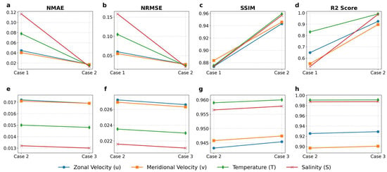
Figure 4.
Comparative validation of different models. (a–d) Comparison between Case 1 and Case 2 for performance changes in different variables (NMAE, NRMSE, SSIM, R2). (e–h) Comparison between Case 2 and Case 3 for performance changes in different variables.
3.5. Model Configuration
The dataset compiled for training, validation, and testing encompasses data from Sub-regions 1 to 4 from 2011 to 2019, comprising a total of 13,140 samples. Following stringent quality control, the dataset was divided according to its spatiotemporal structure into a training set (80%), a validation set (10%), and a test set (10%).
Previous studies on three-dimensional ocean reconstruction have shown that errors are predominantly concentrated in the upper ocean, particularly within the mixed layer and thermocline [45,46,50,53]. The 0–500 m depth range largely encompasses the mixed layer and thermocline across the study regions and was therefore adopted as the selected depth range to specifically evaluate the performance of the reconstruction model. To enable consistent cross-regional comparison, ten representative depth layers (0.49 m, 5.08 m, 13.47 m, 25.21 m, 40.34 m, 65.81 m, 92.33 m, 155.85 m, 318.13 m, and 453.94 m) were uniformly selected, ensuring adequate representation of the three-dimensional ocean structure.
4. Results
4.1. Model Performance of 3DV-Unet
4.1.1. Overall Reconstruction Performance
The 3DV-Unet, trained in two stages, accurately reconstructed temperature (T), salinity (S), and zonal/meridional velocities (u, v) on the full test set. Quantitatively, salinity achieved an RMSE of 0.1123psu with R2 = 0.9698; temperature, an RMSE of 0.3028 °C with R2 = 0.9832; and the zonal and meridional velocities, RMSEs of 0.053m/s and 0.054 m/s with R2 values of 0.9360 and 0.9330, respectively. These results indicate that the model effectively resolves fine-scale oceanic features at eddy-resolving resolution.
To better highlight the superiority of 3DV-Unet, we compared it with recent 3D reconstruction approaches, and the results are summarized in Table 2. Compared with the studies, the proposed 3DV-Unet advances both data specifications and modeling methodology. First, it delivers daily, 3D reconstructions of temperature, salinity, and two horizontal velocity components at 1/12° spatial resolution. Earlier 3D approaches, such as those reported by Jiang et al. (2024), operate at 1° resolution and monthly intervals, which are insufficient for resolving submesoscale processes [51]. Relative to the latest reconstructions by the 2D depth layer at comparable resolution [46,47], 3DV-Unet attains 3D outputs while maintaining competitive accuracy, achieving RMSE values of 0.30 °C for temperature, 0.11 psu for salinity, and 0.054 m/s for both velocity components (all with R2 ≥ 0.93). Secondly, the ViT-3D bottleneck alternately captures dependencies across regions, depths, and variables, improving reconstruction performance. This supports high-resolution 3D reconstruction of multiple ocean variables and serves as a reference for fine-scale coupling analysis.

Table 2.
Recent deep-learning studies and output characteristics of reconstructed ocean physical fields. T: temperature; S: salinity; u: zonal velocity; v: meridional velocity. RMSE and R2 are from the test set. The data for Song et al. (2024) was calculated by averaging the metrics provided for each depth layer in their paper [53].
Analysis of the fine-tuned model further reveals pronounced spatiotemporal heterogeneity in performance across sub-regions and months: errors are larger in dynamically energetic areas such as the South China Sea (Sub-region 4) and smaller in relatively quiescent environments such as the Sea of Okhotsk (Sub-region 1). Examples of representative daily surface field reconstructions are shown in Figure 9.
4.1.2. Ablation Study of Model Components
To evaluate the impact of key architectural components, we conducted an ablation study with three progressively enhanced configurations (Table 3). Case 1 employs a conventional 2D-ViT bottleneck with standard skip connections. Case 2 replaces it with the proposed ViT-3D module, while Case 3 further adds a CA mechanism [57].

Table 3.
Model configurations used in the ablation study, differing in bottleneck structure, skip connections, and input shape; CA stands for Coordinate Attention.
As shown in Figure 4, switching from the 2D-ViT to the ViT-3D (Case 2 vs. Case 1) markedly reduces NRMSE and increases R2 across all variables, indicating lower reconstruction errors and higher predictive skill. Incorporating CA (Case 3) yields additional, though smaller, improvements, confirming that both modules enhance reconstruction performance, with the ViT-3D providing the primary gains.
4.1.3. Analysis of the Multi-Stage Training
We adopted a multi-stage training strategy, first pretraining a fundamental model on all sub-regions and seasons, and then fine-tuning it for specific regions and months. As shown in Figure 5, fine-tuning markedly improves performance in the more stable regimes—Sub-region 1 (Sea of Okhotsk; Figure 5a) and Sub-region 2 (Sea of Japan; Figure 5b)—where median NRMSE drops from 0.020 to 0.015 and R2 increases from 0.96 to above 0.98 for temperature (T) and salinity (S). In these areas, lower eddy kinetic energy and coherent background circulation allow better generalization.
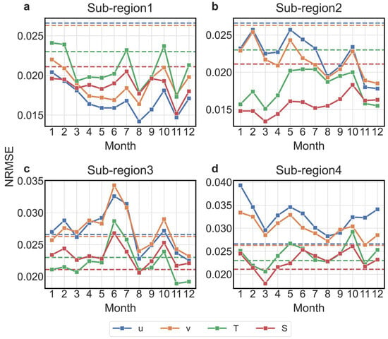
Figure 5.
Monthly variations in normalized RMSE (NRMSE) for reconstructed essential ocean variables in the four sub-regions during 2011–2019. Panels show zonal velocity (u), meridional velocity (v), temperature (T), and salinity (S). Solid lines indicate the results of the fine-tuned 3DV-Unet model, while dashed lines denote the baseline model without multi-stage training. The comparison highlights both regional contrasts and seasonal fluctuations in reconstruction performance.
Sub-region 3 (Kuroshio Extension; Figure 5c) and Sub-region 4 (South China Sea; Figure 5d)—the effect is mixed: salinity and zonal velocity (u) occasionally improve, but meridional velocity (v) and temperature often degrade, with NRMSE exceeding 0.030 and a wider month-to-month spread. The limited size and representativeness of fine-tuning subsets fail to capture complex multi-scale dynamics, leading to higher errors than the fundamental model.
Figure 6 further highlights a consistent disparity between thermohaline and velocity fields. Across all regions, T and S achieve R2 > 0.96 (often > 0.98), indicating robust mass-field reconstruction driven by geostrophic and hydrostatic balance with surface observables. By contrast, u and v yield lower R2 (0.85–0.95) and greater variability, reflecting the challenge of resolving high-frequency, ageostrophic processes. These results suggest a practical paradigm: pretrain on multi-region, multi-season data to establish general priors, and apply fine-tuning selectively where diagnostics indicate likely benefit.
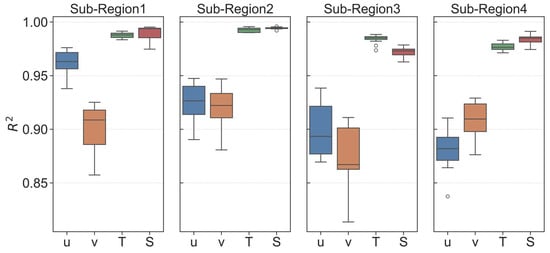
Figure 6.
Monthly R2 values for zonal velocity (u), meridional velocity (v), temperature (T), and salinity (S) across four sub-regions. Each point represents one month.
4.2. Reconstruction Analysis
The annual-mean NRMSE (log10 scale) maps at the surface (Figure 7) reveal geographically coherent error patterns aligned with major circulation regimes. A consistent hierarchy is observed across variables—velocity (u, v) > temperature (T) ≥ salinity (S)—with errors increasing from quiescent basin interiors toward energetic western boundary currents, frontal zones, and shelf regions.
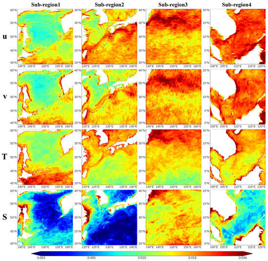
Figure 7.
Annual mean NRMSE spatial distribution for four variables over four sub-regions using a log10 scale of NRMSE; surface (0.49 m) layer.
Sub-region 1 (Sea of Okhotsk) exhibits the lowest errors overall, with uniformly low values in the interior and localized velocity error increases along coasts and the shelf break.
Sub-region 2 (Sea of Japan) shows similarly low, homogeneous errors, with only mild coastal maxima. The relatively stable circulation in these basins supports accurate surface-based inference.
Sub-region 3 (Kuroshio Extension) records the highest errors, especially in velocity, following the jet and its meanders. Strong baroclinic instability, sharp fronts, and frequent positional shifts reduce predictability, while salinity remains more constrained than velocity and temperature.
Sub-region 4 (South China Sea) displays complex patterns, with elevated velocity errors over shelves, straits, and upwelling corridors, and lower errors in the offshore basin. Temperature and salinity errors remain moderate except near dynamic boundaries and freshwater inputs.
Vertically (Figure 8), the RMSE profiles reveal distinct depth-dependent patterns across variables. Errors of zonal and meridional velocities are largest near the surface (~0.05–0.06 m/s) and decrease steadily with depth. Salinity errors are small (<0.1 psu) and reach minima below 300 m. Temperature exhibits a clear subsurface maximum around the thermocline (~50–150 m) before declining at greater depths. Below 200 m, all four variables show weak vertical gradients and consistent minima, indicating strong vertical coherence and the ability of the model to preserve depth-dependent structures.
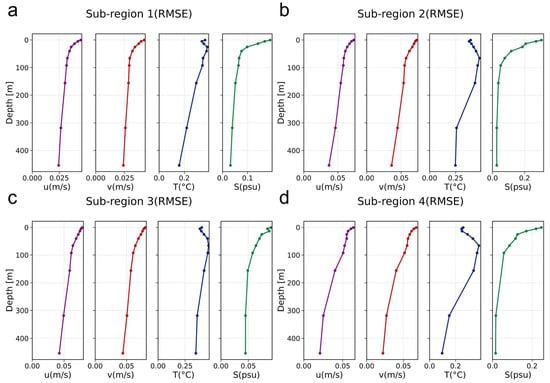
Figure 8.
Annual mean vertical RMSE profiles of reconstructed essential ocean variables (u, v, T, S) for the four sub-regions. Depth-dependent errors are averaged over 2011–2019.
Daily reconstructions for a representative region—the Kuroshio Extension (Figure 9)—further illustrate these patterns. In the Kuroshio Extension, the model reproduces the jet, meanders, and mesoscale eddies with realistic structure, while residuals appear mainly as narrow bands along the jet, indicating positional rather than amplitude errors. Temperature reconstructions retain key frontal and eddy signatures, while salinity remains the most stable variable with generally low residuals offshore. Bias in Figure 9 reveals submesoscale-like features, with filaments aligning with jets and eddy edges. These patterns highlight the challenge of resolving submesoscale processes using only surface observations. Figure 10 compares KE wavenumber spectra for Sub-region 3 (2011–2019) between GLORYS and 3DV-Unet. For both the surface (0.49 m) and the tenth layer (453.94 m), the spectral analysis shows a consistent pattern: the two fields agree at wavelengths > 200 km; over 100–200 km, the model shows a slight negative bias; and in the 20–100 km band, it underestimates energy. The submesoscale discrepancy likely reflects limits of the inputs: the 1/12° daily data provide little information below ~30–40 km, so submesoscale variability is weakly represented in the training signals.
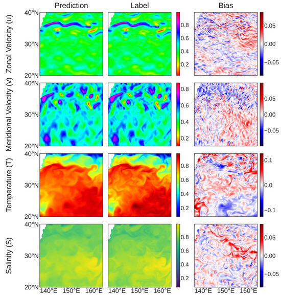
Figure 9.
Comparison of predicted (3DV-Unet) and ground truth (GLORYS12) at the surface layer (0.49 m) on 15 July 2019 in Sub-region 3 (Kuroshio Extension).
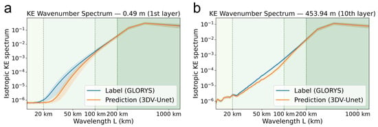
Figure 10.
Kinetic energy (KE) wavenumber spectra at two depths in Sub-region 3; both axes are logarithmic. Blue and orange curves denote the GLORYS and Prediction (3DV-Unet) isotropic KE spectra, and the shaded areas show day-to-day ±1σ variability over 2011–2019. Background shading indicates wavelength regimes (<20 km, 20–100 km, 100–200 km, >200 km), with vertical dashed lines marking the 20, 100, and 200 km transitions. The x-axis is wavelength L (km), and the y-axis is the isotropic KE spectrum. Panels: (a) 0.49 m (1st layer); (b) 453.94 m (10th layer).
To further verify the reconstruction performance, we used 6113 Argo profiles distributed across the four sub-regions for independent validation (Figure 10). To enable direct comparison, a bilinear interpolation scheme was employed to extract values from both the reconstructed fields and the GLORYS reanalysis at the exact spatial positions of each Argo profile.
Compared with Argo observations, the model achieved an R2 of 0.9335 and RMSE of 1.1252 °C for temperature, and an R2 of 0.8784 and RMSE of 0.1378 psu for salinity. The RMSE profiles show close agreement with those of GLORYS across all sub-regions (Figure 10), with temperature errors mainly concentrated near the thermocline and salinity errors remaining low and stable within the upper 500 m. Table 4 further indicates that 3DV-Unet performs on par with or slightly better than GLORYS in most regions, particularly for salinity in Sub-regions 1 and 2, while larger errors in Sub-region 4 reflect the complexity of local dynamics. For comparison, Xie et al. (2025) validated the DUViT model against Argo profiles and obtained temperature RMSEs of 0.257–0.799 °C and salinity RMSEs of 0.045–0.068 psu [46]. Wang et al. (2024) reported RMSEs of 0.590 °C and 0.101 psu using EN4 profiles with CGKDN [42]. Both studies evaluated performance to 2000 m depth, whereas our analysis is restricted to the upper 500 m; since reconstruction errors typically decrease with depth, the results of 3DV-Unet remain highly competitive.

Table 4.
Statistical comparison of 3DV-Unet and GLORYS against Argo profiles across the global domain and four sub-regions, including R2 and RMSE for temperature (°C) and salinity (psu).
As shown in Figure 11, Figure 12 and Figure 13, analysis of error characteristics reveals that most discrepancies between 3DV-Unet and Argo profiles are inherited from the GLORYS reference fields. The similarity in vertical error distributions between the model and GLORYS suggests that while 3DV-Unet achieves strong consistency with the reanalysis product, its reconstructions are also partially constrained by the systematic biases and uncertainties inherent to GLORYS.
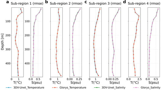
Figure 11.
Depth-dependent RMSE profiles of temperature (T, left) and salinity (S, right) for 3DV-Unet reconstructions (blue and green solid lines) and GLORYS reanalysis (red and magenta dashed lines) in the four sub-regions: (a) Sub-region 1, (b) Sub-region 2, (c) Sub-region 3, and (d) Sub-region 4. The number of Argo profiles used for validation in each region is 97, 1170, 3513, and 1333, respectively.

Figure 12.
Spatial distribution of 6113 Argo profiles used for independent validation in the four sub-regions. Blue dots indicate the locations of all profiles included in the statistical evaluation, and yellow stars mark the positions of the example profiles shown in Figure 13. All Argo profile information used for independent validation, including metadata and matching details, is provided in the Supplementary Materials.
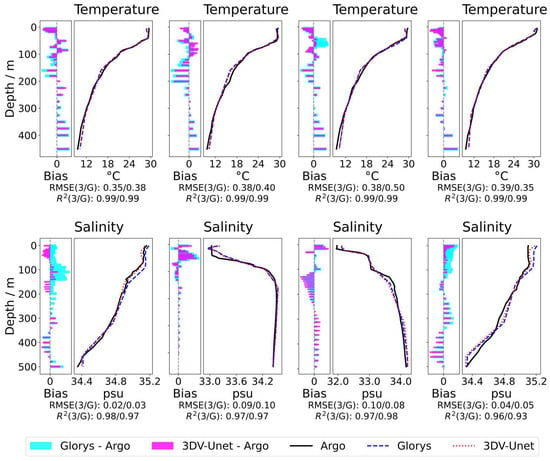
Figure 13.
Example Argo profiles of temperature (top) and salinity (bottom) from the four sub-regions (locations shown in Figure 10). Black lines denote in situ Argo observations, blue dashed lines denote GLORYS reanalysis, and red dotted lines denote 3DV-Unet reconstructions. Left panels show biases (cyan: GLORYS–Argo; magenta: 3DV-Unet–Argo). RMSE and R2 values (3DV-Unet/GLORYS) are reported for each profile.
4.3. Three-Dimensional Eddy Reconstruction
As a case study, we analyzed a representative eddy event to evaluate the ability of 3DV-Unet in reconstructing mesoscale dynamical processes. Figure 13, Figure 14, Figure 15 and Figure 16 depict the sea surface evolution and three-dimensional structure of the same eddy from 1 to 25 March 2015.
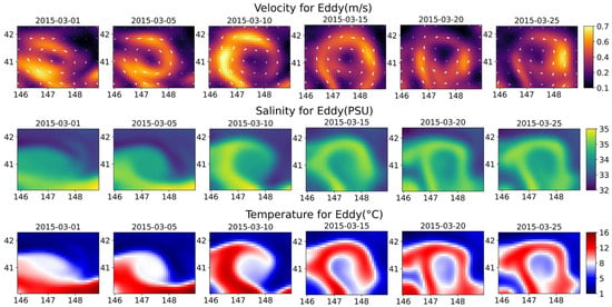
Figure 14.
Sea surface evolution of the eddy from 1 to 25 March 2015. Panels show velocity magnitude with vectors (top), salinity (middle), and temperature (bottom).

Figure 15.
Three-dimensional salinity fields of the same eddy on 1, 10, and 20 March 2015.
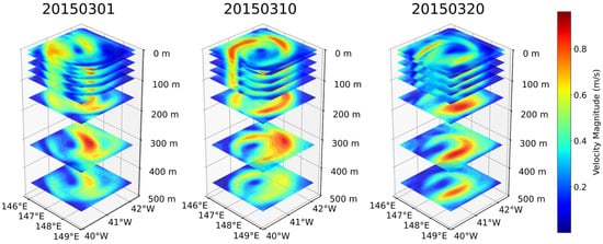
Figure 16.
Three-dimensional velocity magnitude fields of the same eddy on 1, 10, and 20 March 2015.
At the sea surface (Figure 14), the reconstructions clearly reproduce the circulation pattern and the associated temperature and salinity anomalies throughout the eddy’s life cycle, capturing its intensification, maintenance, and decay. In the vertical dimension (Figure 15, Figure 16 and Figure 17), the model reconstructs the penetration of the eddy circulation into the upper 500 m, the doming of isotherms indicative of thermocline displacement, and surface-intensified salinity anomalies that attenuate with depth.
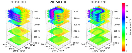
Figure 17.
Three-dimensional temperature fields of the same eddy on 1, 10, and 20 March 2015.
These structural features are consistent with the canonical signatures of mesoscale eddies reported in previous observational and modeling studies, confirming that 3DV-Unet is capable of reconstructing realistic three-dimensional eddy structures and thereby providing a physically consistent representation of mesoscale ocean dynamics.
5. Discussion
The model output results show that errors are primarily concentrated in weak signal features at the submesoscale—such as eddy filaments and submesoscale eddies. The limiting factors are as follows: (i) constraints on ocean remote sensing data: traditional altimeters can only effectively resolve mesoscale signals at the O (100 km) scale, while high-resolution sea surface temperature (SST) data often degrade due to cloud interference and atmospheric noise. Therefore, the input data itself does not contain information about submesoscale dynamic processes; (ii) the model lacks physical mechanism constraints and guidance, making it unable to infer submesoscale fine structures from mesoscale signals. Additionally, due to the blurring effect of the loss function, the model tends to average out submesoscale fine structures rather than capture their details.
In the future, improvements will be made in the following two areas: (i) coupling physical mechanisms, such as adding consistency constraints to the model based on the correlation between variables; (ii) using higher-resolution satellite inputs, such as high-resolution SSH data provided by SWOT, to improve the modeling of submesoscale details.
6. Conclusions
We presented 3DV-Unet, a high-resolution, multi-variable 3D ocean reconstruction model with a dual-attention ViT-3D core. On the full test set, the model achieved RMSEs of 0.3028 °C for temperature (T), 0.1123 psu for salinity (S), 0.0536 m/s for zonal velocity (u), and 0.0543 m/s for meridional velocity (v), with corresponding R2 values of 0.9832, 0.9698, 0.9360, and 0.9330, respectively. Independent validation using 6113 Argo profiles yielded an R2 of 0.933 and RMSE of 1.125 °C for temperature, and an R2 of 0.8784 and RMSE of 0.1378 psu for salinity, demonstrating the model’s capability to reproduce realistic vertical thermohaline structures. These results highlight the potential of 3DV-Unet as a robust framework for high-resolution, physically consistent 3D ocean field reconstruction, with future work focusing on integrating physical-consistency constraints and exploiting higher-resolution satellite observations to further enhance performance.
Supplementary Materials
The following supporting information can be downloaded at: https://www.mdpi.com/article/10.3390/rs17193394/s1. The Supplementary Materials provide basic information of the 6113 Argo profiles used for independent validation, including profile ID, observation date, longitude, and latitude.
Author Contributions
Conceptualization, Q.Z. and H.L.; methodology, Q.Z.; software, Q.Z.; validation, Q.Z.; formal analysis, Q.Z.; investigation, Q.Z.; resources, H.L.; data curation, Z.H. and X.W.; writing—original draft preparation, Q.Z.; writing—review and editing, Q.Z., H.L., H.S., and T.X.; visualization, Q.Z.; supervision, H.L.; project administration, H.L.; funding acquisition, H.L. All authors have read and agreed to the published version of the manuscript.
Funding
This research received no external funding. The APC was funded by the corresponding author’s institutional account.
Data Availability Statement
All data used in this study are publicly available. The SLA, UGOS, VGOS, and SSS datasets are provided by the Copernicus Marine Service (CMEMS; https://marine.copernicus.eu/, accessed on 1 August 2025), SST data are available from NOAA (https://www.ncei.noaa.gov/, accessed on 1 August 2025), and wind data (UWND, VWND) are obtained from the REMSS CCMP Wind Analysis portal (https://www.remss.com/, accessed on 1 August 2025). Precipitation data come from the GMCP dataset (https://data.tpdc.ac.cn/, accessed on 1 August 2025). The GLORYS12v1 reanalysis data used as ground truth are also available via CMEMS. Argo profile data for independent validation are available at https://argo.ucsd.edu/, accessed on 1 August 2025. All datasets are detailed in Table 1 of the manuscript.
Acknowledgments
The authors would like to thank the Copernicus Marine Service, NOAA, REMSS, the National Tibetan Plateau Data Center, and the Argo program for providing open-access datasets used in this research. During the preparation of this manuscript, the authors used ChatGPT (OpenAI, 2024 version) for language editing and text refinement. The authors have reviewed and edited the output and take full responsibility for the content of this publication.
Conflicts of Interest
The authors declare no conflicts of interest.
References
- Intergovernmental Panel on Climate Change (IPCC). The Ocean and Cryosphere in a Changing Climate: Special Report of the Intergovernmental Panel on Climate Change, 1st ed.; Cambridge University Press: Cambridge, UK, 2022; ISBN 978-1-009-15796-4. [Google Scholar]
- Jing, Z.; Fox-Kemper, B.; Cao, H.; Zheng, R.; Du, Y. Submesoscale Fronts and Their Dynamical Processes Associated with Symmetric Instability in the Northwest Pacific Subtropical Ocean. J. Phys. Oceanogr. 2021, 51, 83–100. [Google Scholar] [CrossRef]
- Stewart, R.H. Introduction to Physical Oceanography; Orange Grove Texts Plus: Tucson, AZ, USA, 2009; ISBN 978-1-61610-045-2. [Google Scholar]
- Guo, X.; Gao, Y.; Zhang, S.; Cai, W.; Chen, D.; Leung, L.R.; Zscheischler, J.; Thompson, L.; Davis, K.; Qu, B.; et al. Intensification of Future Subsurface Marine Heatwaves in an Eddy-Resolving Model. Nat. Commun. 2024, 15, 10777. [Google Scholar] [CrossRef]
- Oliver, E.C.J.; Donat, M.G.; Burrows, M.T.; Moore, P.J.; Smale, D.A.; Alexander, L.V.; Benthuysen, J.A.; Feng, M.; Sen Gupta, A.; Hobday, A.J.; et al. Longer and More Frequent Marine Heatwaves over the Past Century. Nat. Commun. 2018, 9, 1324. [Google Scholar] [CrossRef]
- Li, G.; Cheng, L.; Zhu, J.; Trenberth, K.E.; Mann, M.E.; Abraham, J.P. Increasing Ocean Stratification over the Past Half-Century. Nat. Clim. Change 2020, 10, 1116–1123. [Google Scholar] [CrossRef]
- Chen, Y.; Jin, Y.; Liu, Z.; Shen, X.; Chen, X.; Lin, X.; Zhang, R.-H.; Luo, J.-J.; Zhang, W.; Duan, W.; et al. Combined Dynamical-Deep Learning ENSO Forecasts. Nat. Commun. 2025, 16, 3845. [Google Scholar] [CrossRef]
- Kang, N.-Y.; Kim, D.; Elsner, J.B. The Contribution of Super Typhoons to Tropical Cyclone Activity in Response to ENSO. Sci. Rep. 2019, 9, 5046. [Google Scholar] [CrossRef]
- Dong, C.; McWilliams, J.C.; Liu, Y.; Chen, D. Global Heat and Salt Transports by Eddy Movement. Nat. Commun. 2014, 5, 3294. [Google Scholar] [CrossRef]
- Ni, Q.; Zhai, X.; LaCasce, J.H.; Chen, D.; Marshall, D.P. Full-Depth Eddy Kinetic Energy in the Global Ocean Estimated From Altimeter and Argo Observations. Geophys. Res. Lett. 2023, 50, e2023GL103114. [Google Scholar] [CrossRef]
- Wang, A.; Su, H. Spatio-Temporal Neighbors Adaptive Learning with Two-Point Differences for Ocean Subsurface Temperature Reconstruction from 1960 to 2022. Int. J. Digit. Earth 2025, 18, 2500525. [Google Scholar] [CrossRef]
- Zhang, L.; Ma, X.; Wan, X.; Weishuai, X.; Sun, X. Three-Dimensional Thermohaline Reconstruction of Mesoscale Eddies under Remote Sensing Observation: From the Perspective of Deep Learning of Layer Depth Sequences with Fusion of Physical Mechanisms. J. Sea Res. 2025, 205, 102593. [Google Scholar] [CrossRef]
- Duan, Y.; Zhang, H.; Ma, C. Intelligent Inversion of Mesoscale Eddy Temperature Anomaly Profiles Based on Multi-Source Remote Sensing Data. Int. J. Appl. Earth Obs. Geoinf. 2024, 132, 104025. [Google Scholar] [CrossRef]
- Talley, L.D.; Pickard, G.L.; Emery, W.J. (Eds.) Descriptive Physical Oceanography: An Introduction, 6th ed.; Academic Press: Amsterdam, The Netherlands; Boston, MA, USA, 2011; ISBN 978-0-7506-4552-2. [Google Scholar]
- Zhang, Z.; Wang, G.; Wang, H.; Liu, H. Three-Dimensional Structure of Oceanic Mesoscale Eddies. Ocean.-Land-Atmos. Res. 2024, 3, 51. [Google Scholar] [CrossRef]
- Shan, K.; Lin, Y.; Chu, P.-S.; Yu, X.; Song, F. Seasonal Advance of Intense Tropical Cyclones in a Warming Climate. Nature 2023, 623, 83–89. [Google Scholar] [CrossRef]
- Yan, X.; Okubo, A. Three-dimensional Analytical Model for the Mixed Layer Depth. J. Geophys. Res. Oceans 1992, 97, 20201–20226. [Google Scholar] [CrossRef]
- Nian, R.; Zhang, Z.; Ji, Y.; Wang, Y.; Yang, H.; Fu, Z.; Xu, H.; Shi, K.; He, B. Different Types of Surface Chlorophyll Patterns of Oceanic Mesoscale Eddies Identified by AI Framework. J. Geophys. Res. Oceans 2024, 129, e2024JC021176. [Google Scholar] [CrossRef]
- Ding, X.; He, X.; Bai, Y.; Ma, W.; Li, J.; Ye, F.; Yu, S.; Hu, Q.; Gong, F.; Wang, D.; et al. Geostationary Ocean Color Satellite Observations Reveal the Fine Structure of Mesoscale Eddy Dynamics. Remote Sens. Environ. 2025, 320, 114652. [Google Scholar] [CrossRef]
- Meijers, A.J.S.; Bindoff, N.L.; Rintoul, S.R. Estimating the Four-Dimensional Structure of the Southern Ocean Using Satellite Altimetry. J. Atmos. Ocean. Technol. 2011, 28, 548–568. [Google Scholar] [CrossRef]
- Guinehut, S.; Dhomps, A.-L.; Larnicol, G.; Le Traon, P.-Y. High Resolution 3-D Temperature and Salinity Fields Derived from in Situ and Satellite Observations. Ocean Sci. 2012, 8, 845–857. [Google Scholar] [CrossRef]
- Liu, L.; Peng, S.; Wang, J.; Huang, R.X. Retrieving Density and Velocity Fields of the Ocean’s Interior from Surface Data. J. Geophys. Res. Oceans 2014, 119, 8512–8529. [Google Scholar] [CrossRef]
- Wang, J.; Flierl, G.R.; LaCasce, J.H.; McClean, J.L.; Mahadevan, A. Reconstructing the Ocean’s Interior from Surface Data. J. Phys. Oceanogr. 2013, 43, 1611–1626. [Google Scholar] [CrossRef]
- Akbari, E.; Alavipanah, S.; Jeihouni, M.; Hajeb, M.; Haase, D.; Alavipanah, S. A Review of Ocean/Sea Subsurface Water Temperature Studies from Remote Sensing and Non-Remote Sensing Methods. Water 2017, 9, 936. [Google Scholar] [CrossRef]
- Holloway, J.; Mengersen, K. Statistical Machine Learning Methods and Remote Sensing for Sustainable Development Goals: A Review. Remote Sens. 2018, 10, 1365. [Google Scholar] [CrossRef]
- Jeong, Y.; Hwang, J.; Park, J.; Jang, C.J.; Jo, Y.-H. Reconstructed 3-D Ocean Temperature Derived from Remotely Sensed Sea Surface Measurements for Mixed Layer Depth Analysis. Remote Sens. 2019, 11, 3018. [Google Scholar] [CrossRef]
- Maes, C.; Behringer, D.; Reynolds, R.W.; Ji, M. Retrospective Analysis of the Salinity Variability in the Western Tropical Pacific Ocean Using an Indirect Minimization Approach. J. Atmos. Ocean. Technol. 2000, 17, 512–524. [Google Scholar] [CrossRef]
- Chapman, C.; Charantonis, A.A. Reconstruction of Subsurface Velocities from Satellite Observations Using Iterative Self-Organizing Maps. IEEE Geosci. Remote Sens. Lett. 2017, 14, 617–620. [Google Scholar] [CrossRef]
- Rumelhart, D.E.; Hinton, G.E.; Williams, R.J. Learning Representations by Back-Propagating Errors. Nature 1986, 323, 533–536. [Google Scholar] [CrossRef]
- Ke, G.; Meng, Q.; Finley, T.; Wang, T.; Chen, W.; Ma, W.; Ye, Q.; Liu, T.-Y. LightGBM: A Highly Efficient Gradient Boosting Decision Tree. In Proceedings of the Advances in Neural Information Processing Systems; Curran Associates, Inc.: Red Hook, NY, USA, 2017; Volume 30. [Google Scholar]
- Zhang, S.; Deng, Y.; Niu, Q.; Zhang, Z.; Che, Z.; Jia, S.; Mu, L. Multivariate Temporal Self-Attention Network for Subsurface Thermohaline Structure Reconstruction. IEEE Trans. Geosci. Remote Sens. 2023, 61, 4507116. [Google Scholar] [CrossRef]
- Lecun, Y.; Bottou, L.; Bengio, Y.; Haffner, P. Gradient-Based Learning Applied to Document Recognition. Proc. IEEE 1998, 86, 2278–2324. [Google Scholar] [CrossRef]
- Vaswani, A.; Shazeer, N.; Parmar, N.; Uszkoreit, J.; Jones, L.; Gomez, A.N.; Kaiser, Ł.; Polosukhin, I. Attention Is All You Need. In Proceedings of the 31st International Conference on Neural Information Processing Systems; Curran Associates Inc.: Red Hook, NY, USA, 2017; pp. 6000–6010. [Google Scholar]
- Dosovitskiy, A.; Beyer, L.; Kolesnikov, A.; Weissenborn, D.; Zhai, X.; Unterthiner, T.; Dehghani, M.; Minderer, M.; Heigold, G.; Gelly, S.; et al. An Image Is Worth 16 × 16 Words: Transformers for Image Recognition at Scale. arXiv 2020, arXiv:2010.11929. [Google Scholar]
- Liu, Z.; Lin, Y.; Cao, Y.; Hu, H.; Wei, Y.; Zhang, Z.; Lin, S.; Guo, B. Swin Transformer: Hierarchical Vision Transformer Using Shifted Windows. In Proceedings of the 2021 IEEE/CVF International Conference on Computer Vision (ICCV), Montreal, QC, Canada, 10–17 October 2021; IEEE: Piscataway, NJ, USA, 2021; pp. 9992–10002. [Google Scholar]
- Ronneberger, O.; Fischer, P.; Brox, T. U-Net: Convolutional Networks for Biomedical Image Segmentation. In Proceedings of the Medical Image Computing and Computer-Assisted Intervention–MICCAI 2015, Munich, Germany, 5–9 October 2015; Springer: Cham, Switzerland, 2015; Volume 9351, pp. 234–241. [Google Scholar]
- Dong, D.; Brandt, P.; Chang, P.; Schütte, F.; Yang, X.; Yan, J.; Zeng, J. Mesoscale Eddies in the Northwestern Pacific Ocean: Three-Dimensional Eddy Structures and Heat/Salt Transports. J. Geophys. Res. Oceans 2017, 122, 9795–9813. [Google Scholar] [CrossRef]
- Xie, H.; Xu, Q.; Cheng, Y.; Yin, X.; Jia, Y. Reconstruction of Subsurface Temperature Field in the South China Sea from Satellite Observations Based on an Attention U-Net Model. IEEE Trans. Geosci. Remote Sens. 2022, 60, 4209319. [Google Scholar] [CrossRef]
- Su, H.; Jiang, J.; Wang, A.; Zhuang, W.; Yan, X.-H. Subsurface Temperature Reconstruction for the Global Ocean from 1993 to 2020 Using Satellite Observations and Deep Learning. Remote Sens. 2022, 14, 3198. [Google Scholar] [CrossRef]
- Mao, K.; Liu, C.; Zhang, S.; Gao, F. Reconstructing Ocean Subsurface Temperature and Salinity from Sea Surface Information Based on Dual Path Convolutional Neural Networks. J. Mar. Sci. Eng. 2023, 11, 1030. [Google Scholar] [CrossRef]
- Liu, Y.; Wang, H.; Jiang, F.; Zhou, Y.; Li, X. Reconstructing 3-D Thermohaline Structures for Mesoscale Eddies Using Satellite Observations and Deep Learning. IEEE Trans. Geosci. Remote Sens. 2024, 62, 4203916. [Google Scholar] [CrossRef]
- Wang, A.; Su, H.; Huang, Z.; Yan, X.-H. Knowledge-Informed Deep Learning Model for Subsurface Thermohaline Reconstruction from Satellite Observations. IEEE Trans. Geosci. Remote Sens. 2024, 62, 4213416. [Google Scholar] [CrossRef]
- Meng, L.; Yan, C.; Zhuang, W.; Zhang, W.; Geng, X.; Yan, X.-H. Reconstructing High-Resolution Ocean Subsurface and Interior Temperature and Salinity Anomalies from Satellite Observations. IEEE Trans. Geosci. Remote Sens. 2022, 60, 4104114. [Google Scholar] [CrossRef]
- Meng, Y.; Rigall, E.; Chen, X.; Gao, F.; Dong, J.; Chen, S. Physics-Guided Generative Adversarial Networks for Sea Subsurface Temperature Prediction. IEEE Trans. Neural Netw. Learn. Syst. 2023, 34, 3357–3370. [Google Scholar] [CrossRef]
- Zhang, J.; Zhang, X.; Wang, X.; Ning, P.; Zhang, A. Reconstructing 3D Ocean Subsurface Salinity (OSS) from T–S Mapping via a Data-Driven Deep Learning Model. Ocean Model. 2023, 184, 102232. [Google Scholar] [CrossRef]
- Xie, H.; Dong, C.; Xu, Q. Dual U–Vision–Transformer for Reconstructing the Three-Dimensional Eddy-Resolving Oceanic Physical Parameters from Satellite Observations. Int. J. Appl. Earth Obs. Geoinf. 2025, 136, 104382. [Google Scholar] [CrossRef]
- Wang, Q.; Zhang, X.; Wu, X.; Zhang, D.; Qi, J.; Ning, P.; Qiao, X. Deep Learning–Based Eddy-Resolving Reconstruction of Subsurface Temperature and Salinity in the South China Sea. Adv. Atmos. Sci. 2025, 42, 1675–1692. [Google Scholar] [CrossRef]
- Tian, T.; Cheng, L.; Wang, G.; Abraham, J.; Wei, W.; Ren, S.; Zhu, J.; Song, J.; Leng, H. Reconstructing Ocean Subsurface Salinity at High Resolution Using a Machine Learning Approach. Earth Syst. Sci. Data 2022, 14, 5037–5060. [Google Scholar] [CrossRef]
- Chen, Y.; Liu, L.; Chen, X.; Wei, Z.; Sun, X.; Yuan, C.; Gao, Z. Data Driven Three-Dimensional Temperature and Salinity Anomaly Reconstruction of the Northwest Pacific Ocean. Front. Mar. Sci. 2023, 10, 1121334. [Google Scholar] [CrossRef]
- Zhuang, Z.; Zhang, Y.; Zhang, L.; Ruan, W.; Lyu, D.; Yu, J. Reconstructing the Three-Dimensional Thermohaline Structure of Mesoscale Eddies in the South China Sea Using in Situ Measurements and Multi-Sensor Satellites. Remote Sens. 2024, 17, 22. [Google Scholar] [CrossRef]
- Jiang, J.; Wang, J.; Liu, Y.; Feng, L.; Jiang, Q.; Huang, C.; Xiang, L.; Zhang, X. SWO: A Lightweight Window Spatiotemporal Attention Network Reconstructs Subsurface Temperature Structure. IEEE J. Sel. Top. Appl. Earth Obs. Remote Sens. 2024, 17, 19274–19287. [Google Scholar] [CrossRef]
- Su, H.; Zhang, F.; Teng, J.; Wang, A.; Huang, Z. Reconstructing High-Resolution Subsurface Temperature of the Global Ocean Using Deep Forest with Combined Remote Sensing and in Situ Observations. ISPRS J. Photogramm. Remote Sens. 2024, 218, 389–404. [Google Scholar] [CrossRef]
- Song, T.; Xu, G.; Yang, K.; Li, X.; Peng, S. Convformer: A Model for Reconstructing Ocean Subsurface Temperature and Salinity Fields Based on Multi-Source Remote Sensing Observations. Remote Sens. 2024, 16, 2422. [Google Scholar] [CrossRef]
- Su, H.; Qiu, J.; Tang, Z.; Huang, Z.; Yan, X.-H. Retrieving Global Ocean Subsurface Density by Combining Remote Sensing Observations and Multiscale Mixed Residual Transformer. IEEE Trans. Geosci. Remote Sens. 2024, 62, 4201513. [Google Scholar] [CrossRef]
- Sharma, S.; Chaudhari, L. Chapter 9—Vision Transformers and Multi-Sensor Earth Observation. In Deep Learning for Multi-sensor Earth Observation; Saha, S., Ed.; Earth Observation; Elsevier: Amsterdam, The Netherlands, 2025; pp. 201–210. ISBN 978-0-443-26484-9. [Google Scholar]
- Shi, W.; Caballero, J.; Huszar, F.; Totz, J.; Aitken, A.P.; Bishop, R.; Rueckert, D.; Wang, Z. Real-Time Single Image and Video Super-Resolution Using an Efficient Sub-Pixel Convolutional Neural Network. In Proceedings of the 2016 IEEE Conference on Computer Vision and Pattern Recognition (CVPR), Las Vegas, NV, USA, 27–30 June 2016; IEEE: Amsterdam, The Netherlands, 2016; pp. 1874–1883. [Google Scholar]
- Hou, Q.; Zhou, D.; Feng, J. Coordinate Attention for Efficient Mobile Network Design. In Proceedings of the 2021 IEEE/CVF Conference on Computer Vision and Pattern Recognition (CVPR), Nashville, TN, USA, 20–25 June 2021; IEEE: Amsterdam, The Netherlands, 2021; pp. 13708–13717. [Google Scholar]
Disclaimer/Publisher’s Note: The statements, opinions and data contained in all publications are solely those of the individual author(s) and contributor(s) and not of MDPI and/or the editor(s). MDPI and/or the editor(s) disclaim responsibility for any injury to people or property resulting from any ideas, methods, instructions or products referred to in the content. |
© 2025 by the authors. Licensee MDPI, Basel, Switzerland. This article is an open access article distributed under the terms and conditions of the Creative Commons Attribution (CC BY) license (https://creativecommons.org/licenses/by/4.0/).