Seamless Reconstruction of MODIS Land Surface Temperature via Multi-Source Data Fusion and Multi-Stage Optimization

Highlights

What are the main findings?

• A multi-stage framework enables seamless reconstruction of MODIS LST.
• The method ensures high accuracy while retaining spatial–temporal fidelity.

What is the implication of the main finding?

• It offers a generalizable solution for large-scale LST gap-filling.
• It facilitates advanced studies in land–atmosphere and urban climate research.

Abstract

Land Surface Temperature (LST) is a critical variable for understanding land–atmosphere interactions and is widely applied in urban heat monitoring, evapotranspiration estimation, near-surface air temperature modeling, soil moisture assessment, and climate studies. MODIS LST products, with their global coverage, long-term consistency, and radiometric calibration, are a major source of LST data. However, frequent data gaps caused by cloud contamination and atmospheric interference severely limit their applicability in analyses requiring high spatiotemporal continuity. This study presents a seamless MODIS LST reconstruction framework that integrates multi-source data fusion and a multi-stage optimization strategy. The method consists of three key components: (1) topography- and land cover-constrained spatial interpolation, which preliminarily fills orbit-induced gaps using elevation and land cover similarity criteria; (2) pixel-level LST reconstruction via random forest (RF) modeling with multi-source predictors (e.g., NDVI, NDWI, surface reflectance, DEM, land cover), coupled with HANTS-based temporal smoothing to enhance temporal consistency and seasonal fidelity; and (3) Poisson-based image fusion, which ensures spatial continuity and smooth transitions without compromising temperature gradients. Experiments conducted over two representative regions—Huainan and Jining—demonstrate the superior performance of the proposed method under both daytime and nighttime scenarios. The integrated approach (Step 3) achieves high accuracy, with correlation coefficients (CCs) exceeding 0.95 and root mean square errors (RMSEs) below 2K, outperforming conventional HANTS and standalone interpolation methods. Cross-validation with high-resolution Landsat LST further confirms the method’s ability to retain spatial detail and cross-scale consistency. Overall, this study offers a robust and generalizable solution for reconstructing MODIS LST with high spatial and temporal fidelity. The framework holds strong potential for broad applications in land surface process modeling, regional climate studies, and urban thermal environment analysis.

1. Introduction

Land Surface Temperature (LST) is a key variable governing the exchange of energy and moisture at the land–atmosphere interface [1,2]. It plays a critical role in a wide range of applications, including urban heat island assessment, evapotranspiration estimation, near-surface air temperature retrieval, soil moisture monitoring, and global climate change studies [3,4]. Due to the heterogeneous nature of land surface types and the complex spatiotemporal variability of LST, the temperature field often exhibits significant fluctuations across both space and time [5,6,7]. Although ground-based measurements offer high-accuracy local data, their limited spatial coverage and high deployment costs render them impractical for large-scale, spatially consistent, and temporally continuous monitoring [8,9,10].

By contrast, thermal infrared remote sensing provides an efficient means of acquiring long-term, multi-scale LST time series. Among available products, MODIS LST has become a mainstream data source for regional and global studies, owing to its broad spatial coverage, long observational record, and stable radiometric calibration [11,12,13]. However, MODIS LST is fundamentally constrained by its reliance on optical sensing under clear-sky conditions. Surface thermal signals are frequently obscured by cloud cover and atmospheric interference, leading to widespread data gaps. On a global scale, cloudy conditions occur nearly 50% of the time [14,15,16], resulting in substantial portions of the data lacking valid LST observations. These incomplete data severely hinder applications in meteorology, hydrology, and ecology that require high-resolution spatiotemporal continuity.

To mitigate these limitations, numerous LST reconstruction methods have been developed, typically falling into four categories:

(1) Data Fusion-Based Methods. This type of method typically performs spatiotemporal fusion of multi-source remote sensing products (e.g., MODIS, Landsat, and reanalysis data) to simultaneously achieve high temporal and spatial resolutions [17,18]. For instance, Yu et al. [19] utilized pixel-level fusion of MODIS and Landsat, combined with auxiliary ground-based longwave radiation data, to generate daily LST at 100 m resolution with good accuracy and spatial detail in heterogeneous regions. Similarly, Li et al. [20] employed XGBoost to merge MODIS products (TOA and surface radiation-related variables) with multiple reanalysis datasets, producing a global 1 km all-weather instantaneous and daily mean LST dataset (2000–2020) to fill long-term gaps. These methods effectively mitigate the shortcomings of single-source products; however, differences in sensor calibration, observation geometry, and atmospheric conditions often introduce systematic biases or inter-source inconsistencies, reducing the physical consistency of the results.

(2) Empirical Relationship-Based Methods. This category of methods estimates missing LST values by establishing statistical or empirical relationships between LST and environmental variables such as vegetation indices, meteorological factors, and surface reflectance [21,22]. For example, Shiff et al. [23] employed empirical relationships based on climatic seasonality and model anomalies to combine MODIS LST with reanalysis model temperatures (CFSv2), thereby estimating missing pixels caused by cloud cover and generating a global 1 km gap-free LST dataset (including daytime, nighttime, and daily mean). This product exhibits good temporal continuity for long-term trend and climate studies, although residual errors remain under weather and cloud disturbances. Wang et al. [24] observed a seasonal nonlinear relationship between MODIS LST and NDVI in regions such as Lanzhou, and regressed LST against NDVI and NDBI to estimate LST in mixed land-cover pixels. Bartkowiak et al. [25] incorporated meteorological factors (e.g., air temperature, relative humidity, precipitation) and topographic parameters, and applied multiple regression and random forest models to reconstruct MODIS LST gaps at a regional scale, achieving high accuracy under diverse surface conditions. These methods are intuitive in modeling and relatively easy to implement, often delivering high accuracy in local studies. However, they are sensitive to the choice of input factors and model parameters, and may lose generalizability when applied across regions or over long time periods. Moreover, their computational cost can become prohibitive at fine spatial resolutions, limiting their applicability to large-scale, long-term LST reconstruction.

(3) Spatiotemporal Interpolation Methods. This category of methods mainly relies on spatial neighborhood information or temporal series characteristics to fill missing data [26,27,28,29]. Typical techniques include Kriging interpolation, inverse distance weighting (IDW), and the harmonic analysis of time series (HANTS) algorithm. The former leverages spatial autocorrelation for estimation; for example, Guo et al. [30] applied IDW, Kriging, and co-Kriging to fill missing MODIS daytime LST pixels, incorporating DEM and vegetation indices as auxiliary variables to improve interpolation accuracy. The latter restores trends under cloud contamination through time-series fitting; for instance, Xu et al. [31] employed HANTS to remove cloud effects and fill gaps, reconstructing LST time series while effectively preserving seasonal and diurnal variations. The advantage of these methods is that they maintain good spatiotemporal continuity and perform well when the proportion of missing data is relatively low. However, when the missing range is large (e.g., during long-term persistent cloud cover), interpolation methods may produce physically implausible estimates and even cause abnormal fluctuations in the temperature field. Moreover, pure interpolation approaches lack constraints from external environmental factors, making it difficult to reflect the underlying physical processes.

(4) Hybrid Methods. Hybrid approaches attempt to combine two or more strategies to leverage their respective strengths and enhance overall performance [32,33]. For example, Xu et al. [34] proposed a TIR–passive microwave (PMW) data fusion framework, using random forest (RF) as a learning algorithm to merge the all-weather capability of PMW with the spatial detail of TIR, thereby producing high-resolution all-weather LST. Similarly, Gong et al. [35] addressed cloud-contaminated MODIS LST by integrating spatial/temporal constraints with statistical learning, significantly improving the usability of 1 km LST. Such methods can partially overcome the limitations of single strategies and improve reconstruction accuracy under high missing-data scenarios. Nevertheless, due to the lack of strict constraints between different model components, hybrid methods are prone to error accumulation and propagation across stages. In addition, model integration increases complexity and computational burden, limiting the stability and generalizability of these approaches.

In summary, although the above four categories of methods have achieved progress in different scenarios, they still share several common limitations: (1) physical consistency is often difficult to guarantee; (2) reconstruction accuracy tends to be unstable under high missing-data conditions; and (3) errors are prone to accumulate and amplify in integrated approaches. These shortcomings indicate that existing methods still face significant limitations in large-scale, daily LST reconstruction [32,36,37].

To this end, unlike the flexible strategy of Afsharipour et al. [38], our approach adopts a physically constrained, staged pipeline—land cover/elevation-constrained spatial interpolation–complementary RF + HANTS modeling–Poisson equation-based fusion—aimed at controlling error propagation and ensuring boundary seamlessness. This study proposes a multi-stage optimization framework for LST reconstruction. Rather than a simple stacking of multiple models, the framework is designed based on a stepwise progression and physical plausibility. The overall workflow consists of three main stages: (1) Spatial neighborhood interpolation (constrained by land cover and elevation): Under similar environmental conditions, neighboring pixels are used to preliminarily fill short-term or small-scale gaps, thereby improving the physical plausibility of the interpolation results and providing reliable initial inputs for subsequent modeling. (2) Dual modeling (RF + HANTS): Random forest (RF) integrates multiple environmental predictors such as NDVI, NDWI, surface reflectance, DEM, and land cover to capture complex nonlinear relationships of LST and enhance pixel-level reconstruction accuracy; meanwhile, the HANTS algorithm performs harmonic fitting on pixel-level time series, strengthening the seasonal consistency and temporal continuity of the reconstruction results while avoiding unrealistic fluctuations or gaps. (3) Poisson equation-based image fusion: By leveraging gradient constraints and boundary conditions, outputs from different stages are organically combined to ensure smooth transitions and seamless stitching across regions and boundaries, thereby enhancing the overall consistency and visual quality of the reconstructed data.

To validate this framework, we selected Huainan and Jining as representative case study areas. Simulated missing data were generated from MODIS daily LST imagery, and high-resolution Landsat LST products were incorporated as a reference for both qualitative and quantitative assessments.

The design of this multi-stage optimization framework follows a logical sequence of “physical plausibility → temporal stability and pixel-level accuracy → spatial seamlessness,” which effectively reduces the risk of cumulative errors under high missing-data conditions and enhances both interpretability and robustness of the results. Compared with existing integrated methods, the main innovations of this study lie in three aspects: incorporating land cover and elevation constraints into spatial interpolation, proposing complementary modeling with RF and HANTS, and applying a Poisson equation-based fusion approach for seamless integration. In summary, by introducing physically informed spatial constraints and combining machine learning with multi-source remote sensing data, this study advances the traditional reconstruction framework. The proposed method enables seamless and high-accuracy LST reconstruction with strong spatiotemporal consistency, thereby providing a more robust and reliable data foundation for monitoring and analyzing land surface thermal environments.

The structure of this paper is organized as follows: Section 2 introduces the datasets used in this study; Section 3 details the proposed integrated methodology; Section 4 presents experimental results and qualitative/quantitative evaluations; Section 5 discusses the findings; and Section 6 summarizes the main conclusions.

2. Study Area and Data

This study utilized the MODIS Land Surface Temperature product (MOD11A1), the MOD09GA Surface Reflectance product, the Landsat LST product, the CLCD land cover dataset, and the Shuttle Radar Topography Mission (SRTM) Digital Elevation Model (DEM) to conduct high-precision, seamless reconstruction of MODIS LST data from 2016 to 2024. Specifically, MOD11A1 served as the target dataset requiring reconstruction; MODIS Surface Reflectance (SR) and their derived indices were employed to enhance the accuracy, temporal consistency, and spatial continuity of the reconstructed LST data. The CLCD land cover dataset and SRTM DEM were used to impose spatial constraints related to land cover and topography, thereby improving the reconstruction accuracy.

2.1. Study Area

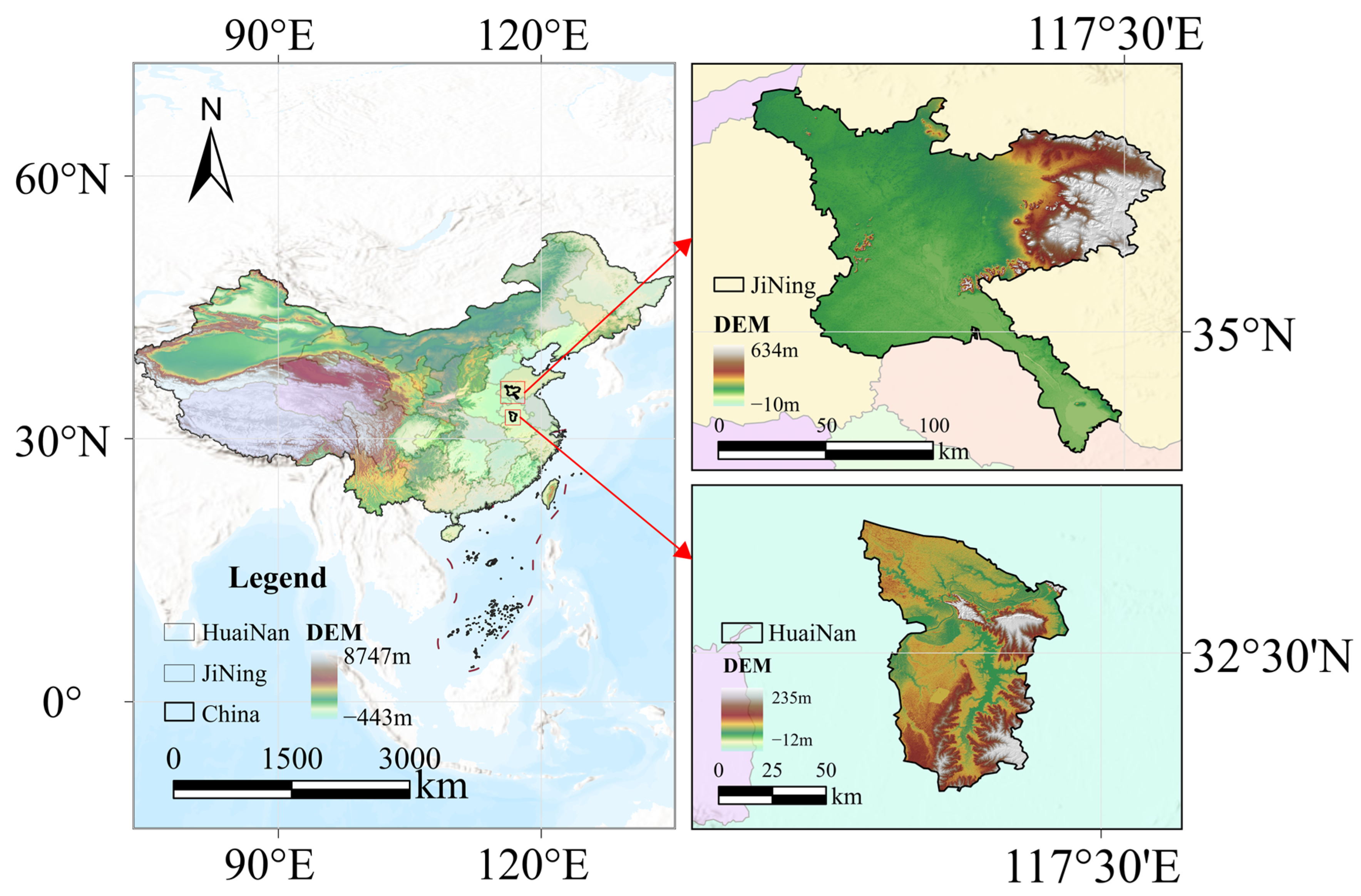
Huainan City in Anhui Province (HN) and Jining City in Shandong Province (JN) are both typical high-groundwater-level regions. Due to their representativeness and pronounced regional differences, they were selected as the study areas (Figure 1).

Huainan (116.36–117.21°E, 31.90–33.01°N) is located in the Huai River Basin in east-central China. It features a humid monsoon climate in the transitional zone between subtropical and warm temperate regions, characterized by hot, rainy summers and cold, dry winters. The area has an average annual temperature of 15.2 °C and an average annual precipitation of approximately 970 mm. Jining (115.53–117.39°E, 34.26–35.57°N) is situated in the southwestern plain of Shandong Province in eastern China. It has a temperate monsoon climate with four distinct seasons, marked by hot, humid summers and cold, dry winters. The average annual temperature ranges from 13 °C to 14.4 °C, with annual precipitation between 597 mm and 819.47 mm.

The two regions differ significantly in terms of geographic location, climate conditions, vegetation cover, and human activity intensity. These disparities result in distinct spatiotemporal patterns of LST and also directly affect the spatial distribution and frequency of cloud cover, further modulating the diurnal and seasonal variations in LST.

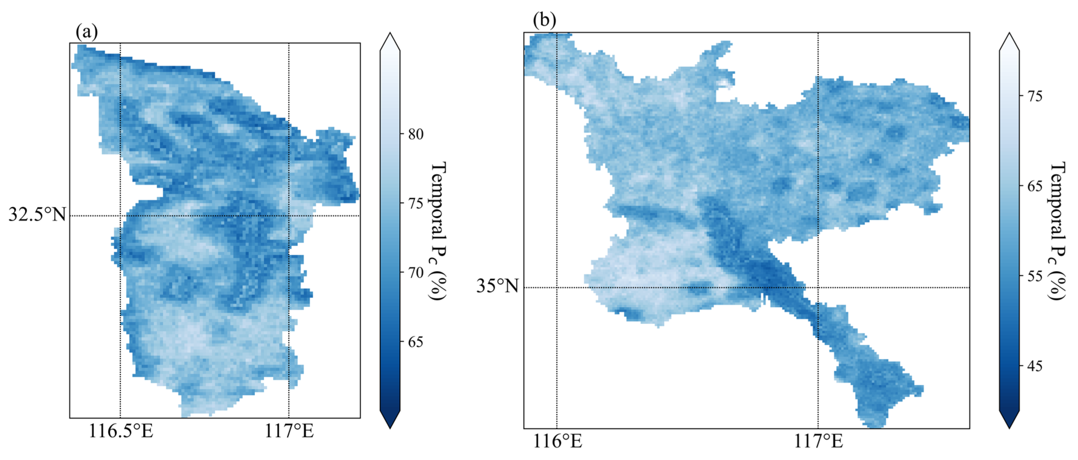
This study computed the daily spatial cloud cover percentage (spatial Pc) and the annual percentage of cloudy days for each pixel (temporal Pc). Cloud pixels were identified based on MODIS daytime LST data.

Figure 2 illustrates the monthly average spatial Pc for both regions in 2018. In Huainan, the monthly spatial Pc ranged from 60.35% to 89.21%, with 237 days exceeding 80% cloud cover. In contrast, the Jining region showed lower values, with spatial Pc ranging from 43.84% to 81.14%, and only 155 days throughout the year had cloud cover above 80%.

Figure 3 displays the distribution of temporal Pc in both regions for 2018. Overall, there was a clear spatial disparity in cloud coverage between the two areas. In Huainan, cloudy conditions were more frequent in the southern part than in the northeast. Jining had an average temporal Pc of 62.68, which is significantly lower than Huainan’s 78.95%.

These notable climatic differences between the two regions provide an ideal comparative context for assessing the performance of LST reconstruction methods under varying cloud cover conditions.

2.2. Data

To map the spatiotemporal distribution of LST from 2016 to 2024, this study integrated multi-source remote sensing data, including the MODIS Land Surface Temperature product (MOD11A1), Surface Reflectance product (MOD09GA), Landsat-based LST, the CLCD land cover product, and the DEM provided by NASA’s Shuttle Radar Topography Mission (SRTM). A summary of the datasets is presented in

Table 1. Data sources.

Data Source	Temporal Resolution	Spatial Resolution	Time Range	Data Type/Usage
MOD11A1	Daily	1 km	2016–2024	Land Surface Temperature (day/night), with QC flag
MOD09GA	Daily	50 0m	2016–2024	Surface Reflectance (Bands 1–7), with QC flag
Landsat LST	16d	100 m	2016–2024	High-resolution LST for validation
CLCD LCC	Year	30 m	2016–2024	Land Cover Classification
SRTM DEM	-	30 m	-	Digital Elevation Model for topographic factors

.

The MOD11A1 product provides daily LST data at a 1 km spatial resolution, covering both daytime and nighttime observations, along with accompanying Quality Control (QC) information. The MODIS sensor onboard the Terra satellite passes over at approximately 10:30 a.m. (daytime) and 10:30 p.m. (nighttime) local time. The QC band is used to assess the usability of the LST data: QC = 00 indicates high-quality data; QC = 01 indicates lower quality or potentially unreliable data; QC = 10 means the data could not be retrieved due to cloud contamination; and QC = 11 signifies other data acquisition failures. To ensure data quality and analytical reliability, this study retained only pixels with QC = 00 [39].

The MOD09GA product provides MODIS surface reflectance data for bands 1–7 at a 500 m resolution, with per-band quality flags. Pixels with QC = 0 (i.e., all bands in ideal condition) were selected to generate daily reflectance composite data. From this, the Normalized Difference Vegetation Index (NDVI) and the Normalized Difference Water Index (NDWI) were calculated to capture vegetation and water body characteristics.

Additionally, 30 m resolution SRTM DEM data and land cover data from the China Land Cover Dataset (CLCD) were used as auxiliary variables for LST reconstruction and analysis.

Landsat LST products were also introduced as an external validation reference for the MODIS LST reconstruction results. The Landsat satellites provide higher spatial resolution (approximately 100 m) LST data, which help assess the accuracy and spatial detail recovery of the MODIS-based reconstruction.

All remote sensing data acquisition and preprocessing were conducted on the Google Earth Engine (GEE) platform. To ensure consistency in spatial resolution, all continuous variables (such as LST, reflectance, and elevation) were resampled to 1 km using bilinear interpolation, matching the resolution of MODIS LST products [40]. For the categorical land cover data, nearest neighbor interpolation was used to preserve classification accuracy [41].

3. Methods

3.1. LST Reconstruction

The daily MODIS LST product is frequently affected by high cloud cover in both time and space, leading to widespread pixel gaps and continuous missing values in the time series. This significantly limits its applicability in spatiotemporally continuous monitoring. Therefore, incorporating auxiliary data to improve the completeness and accuracy of LST reconstruction is of great importance.

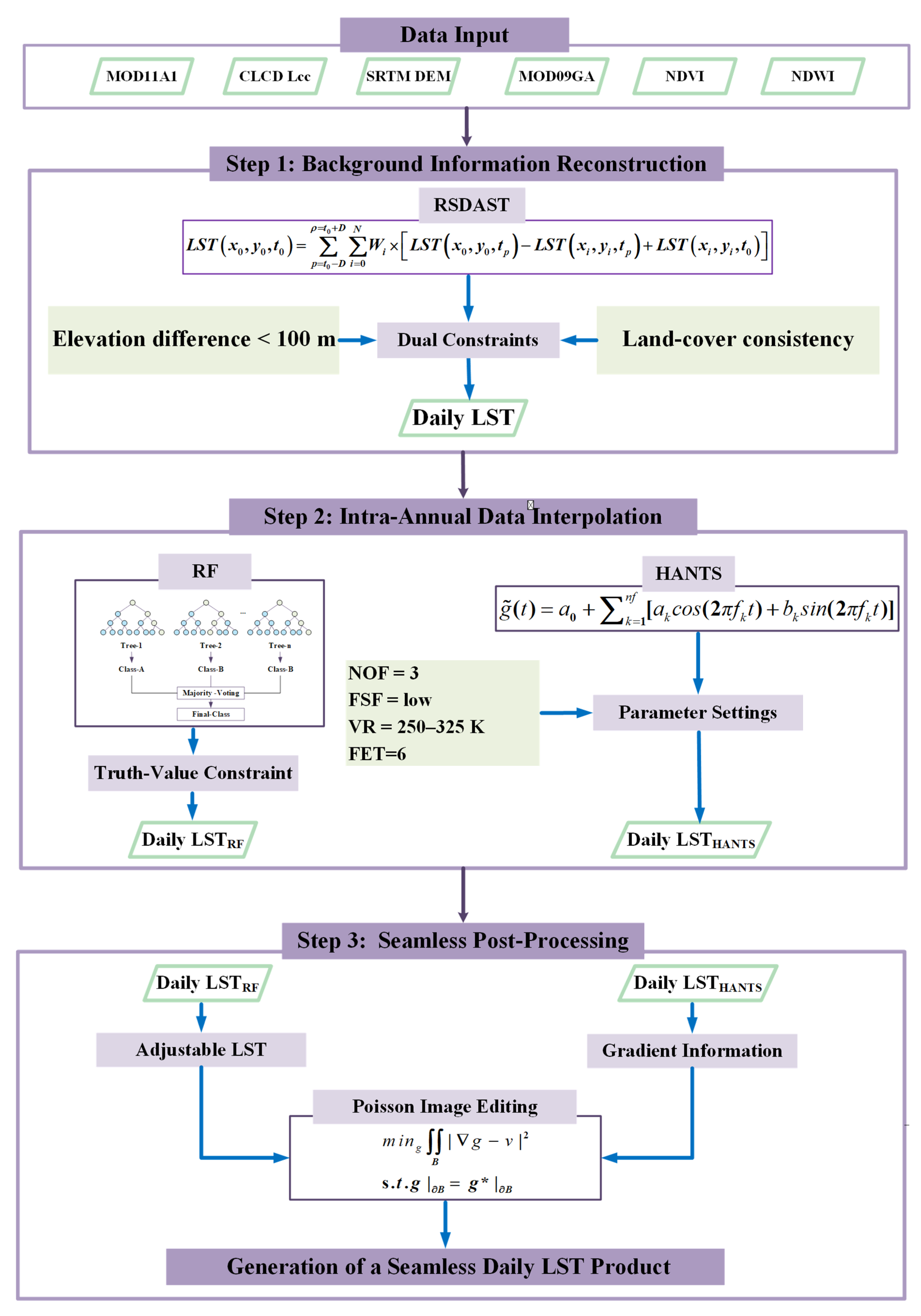
Given that LST is highly sensitive to terrain features—especially elevation—and is influenced by changes in land cover types, this study integrates a range of auxiliary datasets to support high-quality daily LST reconstruction. These include the MODIS Surface Reflectance product (MOD09GA), SRTM DEM, multi-year daily mean LST, CLCD land cover classification (LCC), NDVI, and NDWI. Their high temporal resolution, multispectral information, and good availability provide strong support for spatiotemporal interpolation of LST, and the overall technical roadmap is illustrated in Figure 4.

3.1.1. Background Information Reconstruction

The background information reconstruction process is shown in Figure 4 (Step 2). In geographic space, the relationship between two spatial units is closely linked to their spatial distance. According to the First Law of Geography, nearby pixels tend to exhibit more similar surface characteristics. When two pixels are sufficiently close, they are typically subjected to similar weather conditions—such as solar radiation, air temperature, and precipitation—resulting in enhanced synchrony in Land Surface Temperature (LST) variation.

Based on this principle, Sun et al. [42] proposed a model assuming that the temperature difference between a cloud-contaminated pixel and its neighboring clear-sky pixels remains stable over time, expressed as follows:

$$LST\left(x_0,y_0,t_0\right)-\mathrm{L}\mathrm{S}\mathrm{T}\left(x_i,y_i,t_0\right)=\mathrm{L}\mathrm{S}\mathrm{T}\left(x_0,y_0,t_p\right)-\mathrm{L}\mathrm{S}\mathrm{T}\left(x_i,y_i,t_p\right)$$

(1)

where ${(x}_0,y_0)$ denote the coordinates of the target pixel to be reconstructed, while $(x_i,y_i)$ represent the coordinates of its valid neighboring clear-sky pixels. $t_0$and $t_p$ are the current time and the reference time, respectively.

Building on this assumption, they developed the RSDAST model (Reconstruction based on Spatial and Temporal Adjustment of Surface Temperature differences) [43,44], which is expressed as follows:

$$LST\left(x_0,y_0,t_0\right)={\sum }_{p=t_0-D}^{\rho =t_0+D} {\sum }_{i=0}^N W_i\times \left[LST\left(x_0,y_0,t_p\right)-LST\left(x_i,y_i,t_p\right)+LST\left(x_i,y_i,t_0\right)\right]$$

(2)

where $LST\left(x_0,y_0,t_0\right)$ is the pixel to be reconstructed, $\left(x_i,y_i\right)$ are the coordinates of valid neighboring pixels, $t_0$and $t_p$ represent the current and reference times, respectively, $D$ is the half-width of the temporal window, $N$ is the number of candidate pixels, and $Wi$ is the weight assigned to each neighboring pixel, calculated as follows:

$$W_i={\displaystyle \frac{1}{D_i\cdot S_i}}/{\sum }_{i=1}^N \left({\displaystyle \frac{1}{D_i\cdot S_i}}\right)$$

(3)

In this formula, $D_i=\sqrt{{\left(x_i-x_0\right)}^2+{\left(y_i-y_0\right)}^2}$ represents the spatial distance (distance factor), and $S_i=\left|LST\left(x_0,y_0,t_p\right)-LST\left(x_i,y_i,t_p\right)\right|+1$ represents the similarity factor, with the addition of 1 to avoid division by zero when similarity is perfect. A smaller $S_i$implies higher similarity between the surface conditions of the candidate and target pixels at the reference time, thus contributing a higher weight.

To enhance the model’s adaptability in heterogeneous landscapes and complex terrains, this study introduced dual constraints—land cover and elevation—as prior conditions for selecting candidate pixels: (1) Land Cover Consistency: Candidate pixels must have the same land cover type as the central pixel, determined using the CLCD land cover product through per-pixel registration and matching. (2) Elevation Difference Constraint: The elevation difference between the candidate and the central pixel must not exceed $\pm 100 \mathrm{m}$. SRTM DEM data were resampled to match the spatial resolution of the LST imagery. Weight calculation and temperature interpolation were only performed when at least five valid neighboring pixels $N\ge 5$ satisfied both constraints. Otherwise, reconstruction for that pixel was skipped.

For pixels that failed to meet the reconstruction conditions, a backup filling method was applied using “stable pixels”—areas where land cover remained unchanged over multiple years, as identified from the CLCD dataset. For these areas, multi-year daily mean LST composites were used as auxiliary data to fill gaps. This approach utilizes spatiotemporal patterns embedded in long-term average LST, thereby enhancing the continuity and robustness of the reconstructed dataset.

3.1.2. Intra-Annual Information Reconstruction

To fully leverage the respective advantages of temporal smoothing and high-resolution spatial reconstruction, this study designed two different types of reconstruction outputs.

First, the time-series interpolated data generated by the HANTS algorithm [45,46,47] is primarily used to fill continuous gaps in the time series and eliminate random noise, making the LST data more continuous and smooth in the temporal dimension. This allows them to accurately reflect seasonal and periodic variation patterns, and their performance and applicability have been evaluated across regional to global scales [48,49]. Second, spatially reconstructed data generated by the random forest (RF) model focus on capturing the complex nonlinear relationships between multi-source auxiliary features and Land Surface Temperature, thereby improving the spatial prediction accuracy and enhancing the representation of missing pixels.

The combination of both approaches not only avoids the limitations of using a single method in either the temporal or spatial domain but also uses the smoothed time-series data produced by HANTS as gradient adjustment information to assist in optimizing the spatial distribution of LST reconstructed by RF. This enhances the overall temporal consistency and spatial accuracy of the reconstruction results, achieving a more comprehensive and reliable filling of missing LST values.

(1) HANTS Interpolation

The background information reconstruction process can only provide an initial filling of missing values. When reference data are missing across all years, gaps still remain in the results. Therefore, at the pixel level, the HANTS algorithm was introduced based on intra-annual time information to achieve more thorough gap filling.

HANTS (Harmonic ANalysis of Time Series) is based on Fourier transformation and has been widely used for reconstructing remote sensing quantitative product time series, with over 20 years of application history. Its reconstruction mechanism involves removing random noise caused by atmospheric interference and sensor issues.

Mathematically, it is expressed as the sum of a constant term and multiple sine and cosine functions, as follows:

$$\tilde{g}(t)=a_0+{\sum }_{k=1}^{nf}[a_{k}cos(2\pi f_{k}t)+b_{k}sin(2\pi f_{k}t)]$$

(4)

$$g(t)=\tilde{g}(t)+\epsilon (t), \mathrm{t}=1,\dots ,N$$

(5)

In this context, $g(t)$ represents the original time series, $\tilde{g}(t)$ is the reconstructed series, and $\epsilon (t)$denotes the error sequence. $t$ is the time point, and $N$ is the length of the time series. $aₖ$and$bₖ$are the coefficients of the trigonometric functions with frequency $fₖ$, and $nf$ is the number of harmonics involved in the fitting.

HANTS is an iterative process, with its core steps as follows: (1) The pixels whose values fall outside the valid range are excluded. For example, for LST data, the valid range is typically 250–325 K; pixel values outside this range will be excluded. (2) For the remaining valid pixels, the least squares method is applied to fit the above equation. (3) This process is repeated until the termination criteria are met. The termination conditions include the following: the maximum error between the current fitted curve and the input data is smaller than a predefined threshold, or the remaining valid observations are insufficient to support the fitting process.

Numerous studies have demonstrated that LST exhibits pronounced seasonal periodicity. Therefore, this study applied the HANTS algorithm to reconstruct the time series. For parameter configuration, we first referred to the settings proposed by Y. Xu and Y. Shen [50], and set the valid value range to 250–325 K with the FET fixed at 6 K. Since the number of frequencies (NOFs) has the most significant impact on reconstruction accuracy, a sensitivity analysis was further conducted. Following the approach of Yang et al. [16], two high-quality (QA = 00) LST scenes from the HN and JN regions (30 March and 12 October 2018) were selected. Artificial gaps were generated through simulated cloud contamination, and the missing pixels were reconstructed using HANTS. Reconstruction accuracy was then evaluated by comparing reconstructed and original values using RMSE and AAD. The results showed that both metrics decreased as NOF increased from 1 to 3, indicating improved reconstruction accuracy, but increased again when NOF exceeded 3. Notably, at NOF = 3, RMSE and AAD reached their minimum values, suggesting that this configuration achieves the best balance between fitting accuracy and robustness. Therefore, the final HANTS parameter settings were determined as NOF = 3 and FET = 6 (see

Table 2. Parameter settings of the HANTS algorithm.

Parameters	Description	Values
NOF	Number of frequencies	3
SF	The suppression flag indicating whether high or low values should be rejected during curve fitting	low
low	Low threshold	250
high	High threshold	325
FET	Fit error tolerance	6

), ensuring both accuracy and reliability of the reconstructed LST data.

(2) Pixel-wise Reconstruction Using Random Forest

Random forest (RF) is a non-parametric regression algorithm based on the principle of ensemble learning. It constructs a multitude of decision trees, each trained on a subset of the input data, and aggregates their predictions to enhance overall accuracy while effectively mitigating the risk of overfitting. During model training, RF applies bootstrap sampling with replacement to generate diverse training subsets and randomly selects a subset of features at each node to determine the optimal split. This strategy improves the model’s generalization ability and robustness. Owing to its strong adaptability to high-dimensional and multi-source inputs, as well as its inherent tolerance to missing values, RF has been widely adopted for spatiotemporal reconstruction and parameter retrieval in remote sensing applications [51,52].

In this study, we implemented the RF-based reconstruction framework using the scikit-learn library in Python 3.10 to address data gaps in daily MODIS LST products. To ensure spatial consistency, the original MODIS LST data and auxiliary datasets—including NDVI, NDWI, land cover (CLCD), elevation (DEM), and MOD09GA surface reflectance—were resampled to a common spatial resolution of 1 km. This alignment step ensured that all input variables were spatially co-registered.

Invalid and noisy pixels were excluded based on a combination of LST value range constraints and the vector boundary of the study area, supported by MODIS quality control flags. This pre-filtering step substantially reduced the influence of anomalous observations on model performance.

For feature construction, a comprehensive set of physically meaningful predictors was assembled by integrating DEM, CLCD, NDVI, NDWI, and multiple MODIS reflectance bands. In addition, multi-year daily mean LST was incorporated as a prior input to provide background thermal context. Considering the varying temporal sensitivities of individual spectral bands to LST dynamics, a band-wise modeling strategy was adopted, whereby separate RF models were trained for each spectral band to meet the demands of annual-scale reconstruction.

To further improve model performance and generalization ability, the dataset was randomly divided into training and validation subsets with an 80:20 ratio. In the optimization of random forest hyperparameters, this study focused on key parameters including the number of trees (n_estimators), maximum depth (max_depth), and minimum samples required for splitting (min_samples_split). A grid search (GridSearchCV) combined with three-fold cross-validation was employed to systematically explore the predefined parameter space, using the negative mean squared error (MSE) as the scoring metric, together with RMSE and MAE on the validation set for comprehensive evaluation. The results indicated that model accuracy stabilized when n_estimators exceeded 200, while a maximum depth around 20 provided the best balance between fitting capacity and generalization ability; the optimal value for min_samples_split was 2. Accordingly, the final configuration was set to n_estimators = 200, max_depth = 20, and min_samples_split = 2. This configuration ensured high predictive accuracy while maintaining computational efficiency and robustness. The optimized models exhibited strong predictive performance and stability across multiple independent test regions, further confirming the effectiveness and scalability of the RF approach for reconstructing missing MODIS LST pixels.

This subsection produces two outputs: (1) the LST data reconstructed using HANTS; and (2) the LST data reconstructed using RF. Both datasets serve as inputs to Step 3, where the RF results provide modifiable LST constrained by real observations, while the HANTS results provide the gradient vector field.

3.1.3. Seamless Post-Processing

Through intra-annual time-series reconstruction, LST data with improved spatiotemporal continuity were obtained. However, gaps still exist at the boundaries between original valid regions and reconstructed areas, which affect the overall seamlessness of the dataset. To address this issue, this study introduces a seamless fusion algorithm based on the Poisson equation. This algorithm solves a Poisson partial differential equation with Dirichlet boundary conditions, aiming to find a function whose gradient field is closest to a target vector field under given boundary gradient information and boundary values, thereby achieving smooth transitions at the boundary and seamless data stitching.

The core of this algorithm is the Poisson partial differential equation with Dirichlet boundary conditions. These boundary conditions define the Laplacian of the unknown function over the region of interest, as well as its values on the boundary. Essentially, this is a minimization problem under the L2 norm, where the goal is to find a function whose gradient best approximates a given target vector field under the specified boundary constraints.

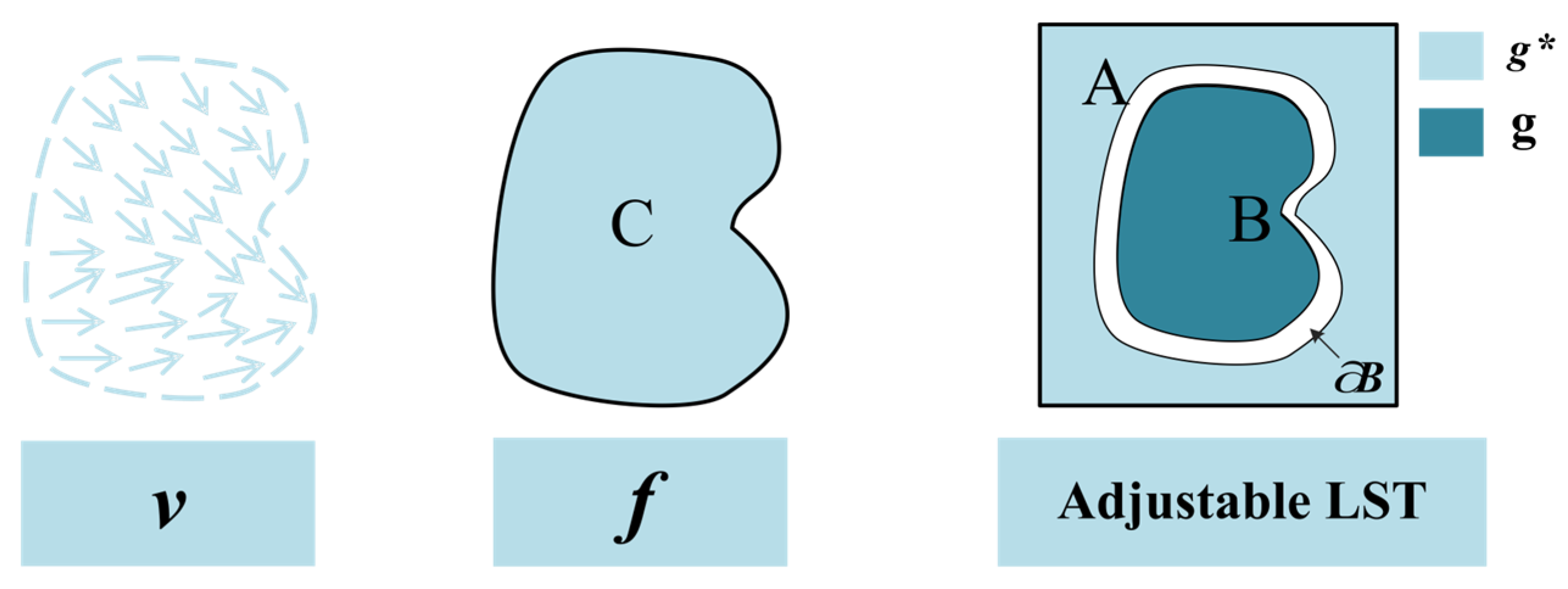
To facilitate understanding, Figure 4 and Figure 5 (Step 3) illustrate the meaning of various symbols: B denotes the reconstructed region to be fused, with its boundary represented by ∂B. g is the unknown function to be solved. g* is the known function defined in the valid region A. v is the guidance vector field derived from a function f in the source region C.

The basic requirement of image fusion is to ensure that the merged image is as smooth as possible without visible boundaries. Therefore, the interpolant g within region B is obtained by solving the following optimization problem:

$${min}_g{\iint }_B|\nabla g-\mathit{v}{|}^2$$

(6)

$$\begin{array}{c}{s.t.g|}_{\partial B}=g^{\ast }{|}_{\partial B}.\end{array}$$

(7)

where ∇ = (∂/∂x,∂/∂y) is the gradient operator. The corresponding Euler–Lagrange equation leads to the classical Poisson formulation with Dirichlet boundary conditions:

$$\Delta g=divv$$

(8)

$$s.t.{g|}_{\partial B}={g^{\ast }|}_{\partial B}$$

(9)

where Δ is the Laplacian operator; $div v = (\partial u/\partial x + \partial v/\partial y)$, where $v = (u, v)$ represents the two components of the guidance vector field. This forms the fundamental machinery of Poisson editing.

This procedure is applied to all reconstructed images, since boundary seams are unavoidable. A binary mask file generated during preprocessing is used to identify the fusion region: Pixels in the reconstructed area are assigned a value of 1, while those in the original valid area are assigned a value of 0. If the mask contains only 0 s or only 1 s, the corresponding image is excluded from this step. The transition between 0 and 1 defines the boundary ∂B, which corresponds to the seam location.

In this step, B represents the region reconstructed by RF and constrained by valid observations, where pixel values need further adjustment. The guidance vector field v is derived from region C, which does not necessarily contain true values but must provide reliable gradient information. For example, the intermediate product reconstructed by HANTS in Step 2 can be used to construct v. Although the absolute values of HANTS reconstruction may deviate, its gradient structure is generally robust and suitable for guidance.

In summary, this step performs a secondary adjustment of pixel values in the reconstructed region. By enforcing gradient constraints and Dirichlet boundary conditions, it effectively smooths the boundary transition and achieves seamless integration between original and reconstructed areas.

3.2. Evaluation Metrics

The first evaluation metric is the Pearson correlation coefficient (CC), which is used to measure the degree of similarity between the reconstructed values and the original values. It is defined as follows:

$$CC={\displaystyle \frac{{\sum }_{j=1}^M(g_{re(j)}-g_{\bar{r}e})(g_{or(j)}-g_{\bar{o}r})}{\sqrt{{\sum }_{j=1}^M(g_{re(j)}-g_{\bar{r}e}{)}^2(g_{or(j)}-g_{\bar{o}r}{)}^2}}}$$

(10)

Here, $g_{re(j)}$ and $g_{or(j)}$ represent the reconstructed and original values of the $j$ contaminated pixel, respectively. $g_{\bar{r}e}$ and $g_{or}$ denote their corresponding mean values, and $M$ is the total number of contaminated pixels. A higher $CC$ value indicates a stronger similarity between the two sets of data.

The second evaluation metric is Bias, which measures the systematic deviation between the reconstructed values and the original values. It is defined as follows:

$$Bias ={\displaystyle \frac{1}{M}}{\sum }_{j=1}^M(gre(j)-gor(j))$$

(11)

A Bias value closer to zero indicates that the reconstruction results do not systematically overestimate or underestimate the original values.

The third evaluation metric is the root mean square error (RMSE), which quantifies the overall deviation between the reconstructed values and the original values. It is defined as follows:

$$RMSE=\sqrt{{\sum }_{j=1}^M(g_{re(j)}-g_{or(j)}{)}^2/(M-1)}$$

(12)

Here, M denotes the total number of contaminated pixels, and $g_{\mathrm{r}\mathrm{e}(j)}$ and $g_{\mathrm{o}\mathrm{r}(j)}$ represent the reconstructed and original values of the $j$ missing pixel, respectively. A smaller RMSE value indicates that the reconstructed results are closer to the original data, implying better reconstruction performance.

4. Results

4.1. Visual Assessment of Reconstruction in Simulated Missing Regions

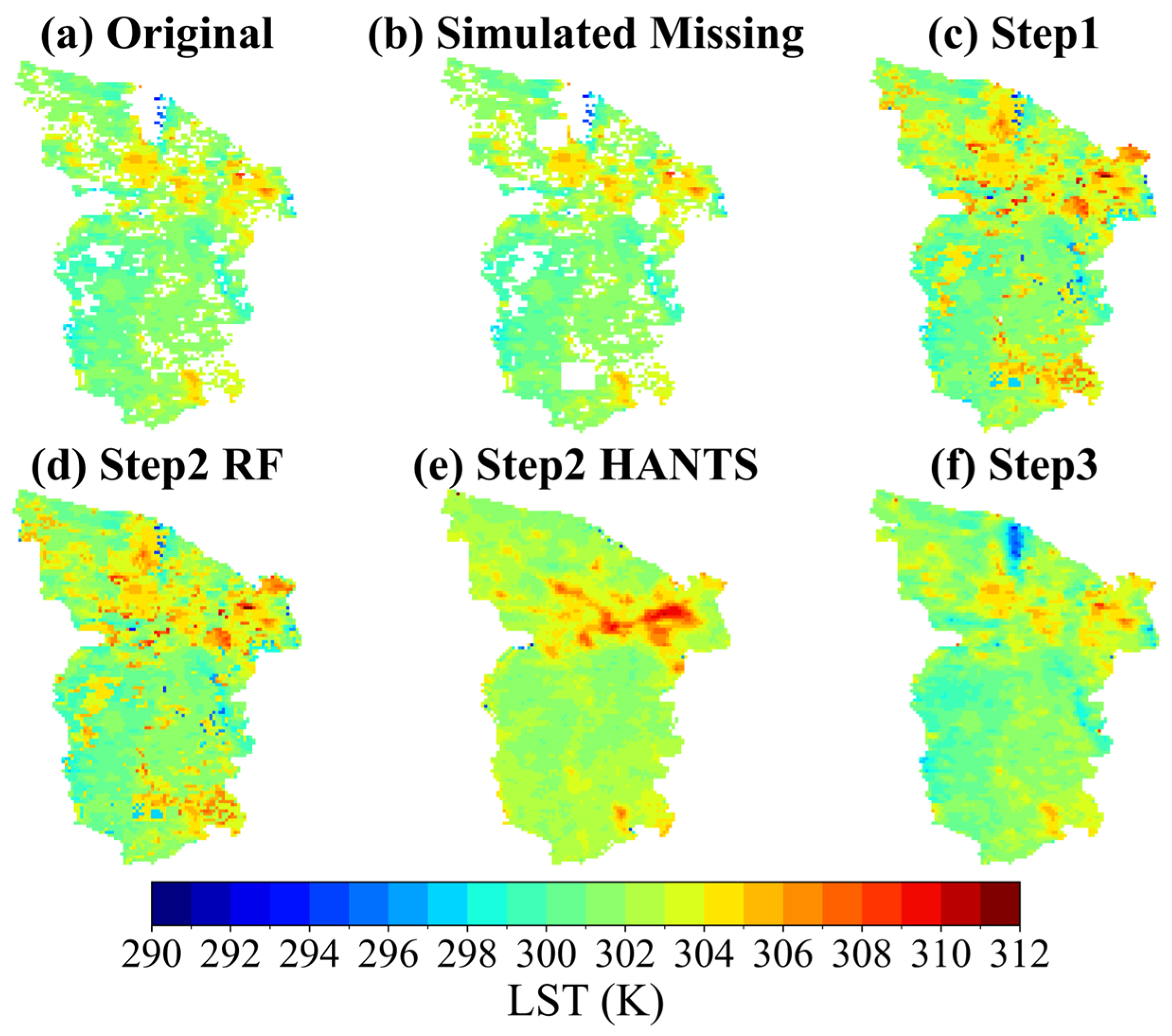
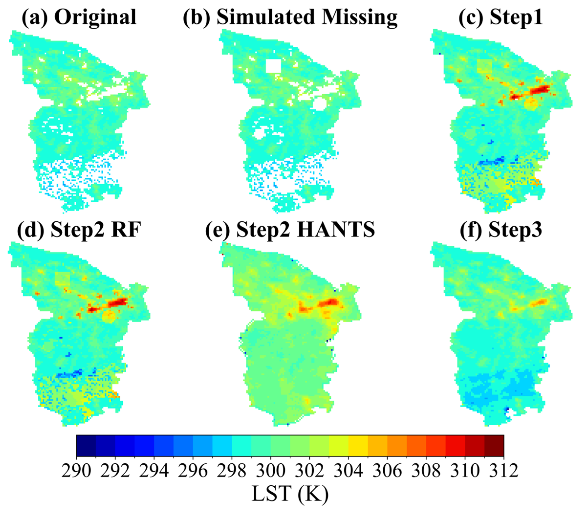
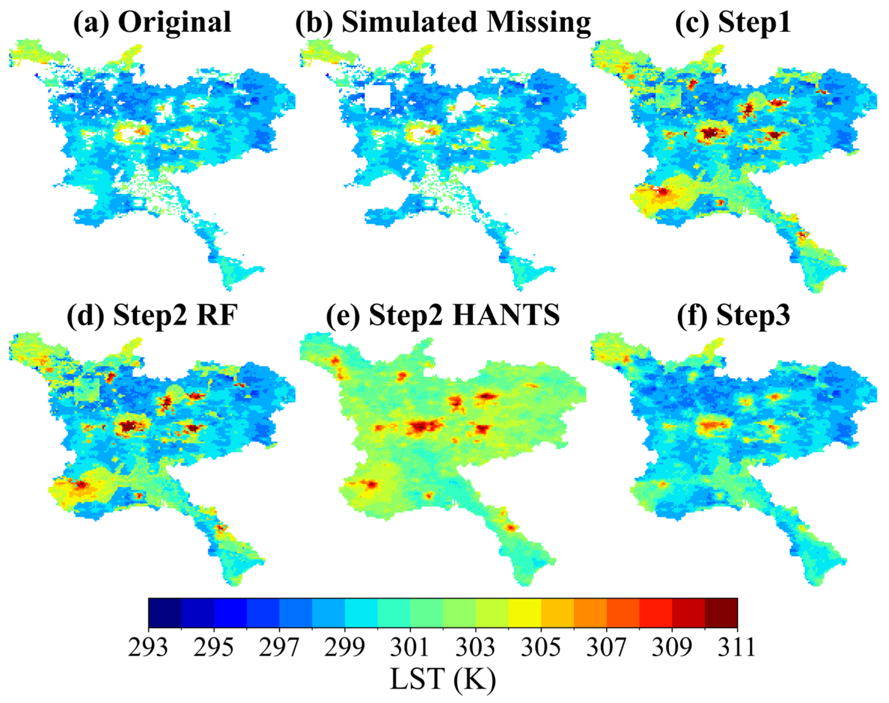
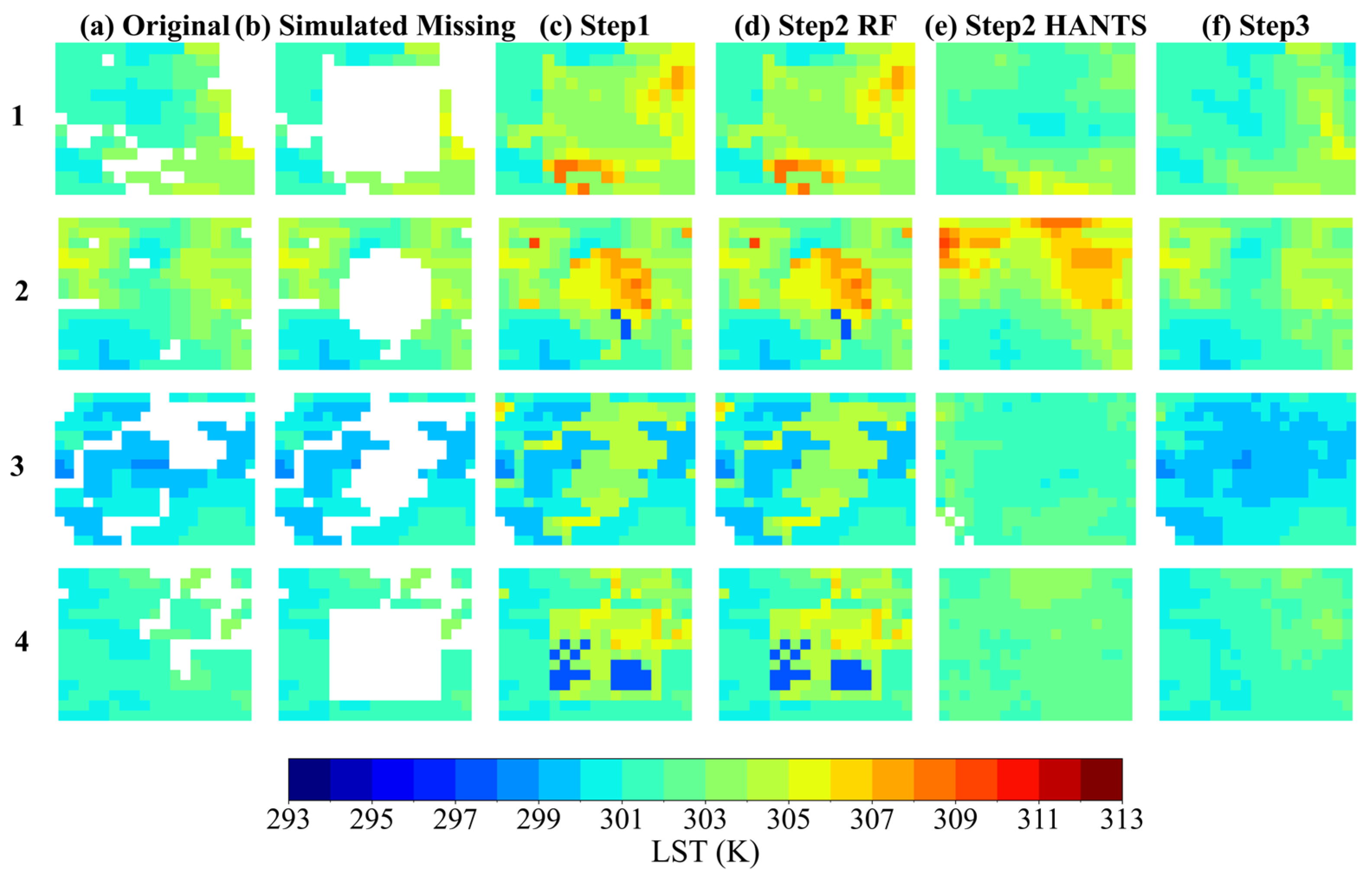
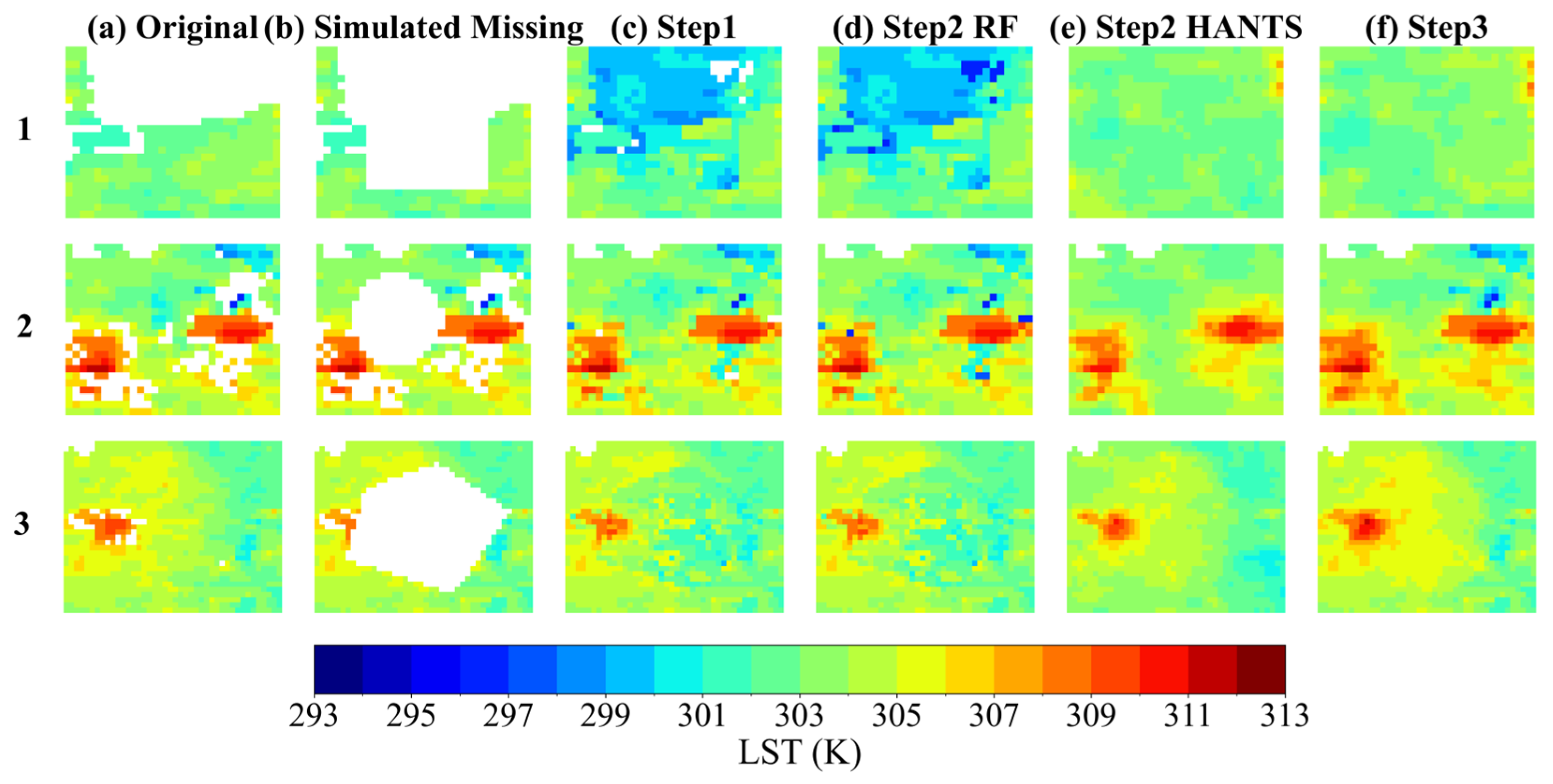
To comprehensively evaluate the effectiveness of the proposed integrated LST reconstruction method, this study selected HN and JN as representative regions. Under clear-sky conditions, typical daytime and nighttime MODIS LST images were analyzed from both qualitative and quantitative perspectives. The selected images were acquired on 12 August (HN-Day), 24 August (HN-Night), 26 August (JN-Day), and 25 August (JN-Night) in 2018. For evaluation, simulated missing areas were generated by intentionally masking portions of high-quality MODIS pixels, ensuring that reliable reference data remained available for comparison. This design not only guarantees the credibility of the reference dataset but also enables a rigorous assessment of the robustness of the reconstruction method under various missing patterns. Figure 6, Figure 7, Figure 8 and Figure 9 illustrate the full-scene reconstruction performance at each step, while Figure 10, Figure 11, Figure 12 and Figure 13 provide zoomed-in comparisons of three or four representative missing regions.

Table 3. Evaluation metrics for reconstructed daytime LST (12 and 26 August 2018).

Day	HN (12 August 2018)			JN (26 August 2018)
	CC	Bias	RMSE	CC	Bias	RMSE
Step 1	0.727	−0.295	1.195	0.715	−1.154	1.634
Step 2 HANTS	0.713	−0.814	1.417	0.922	−0.113	0.561
Step 2 RF	0.721	−0.283	1.094	0.720	−1.134	1.600
Step 3	0.932	0.049	0.599	0.925	0.426	0.718

and

Table 4. Evaluation metrics for reconstructed nighttime LST (24 and 25 August 2018).

Night	HN (24 August 2018)			JN (25 August 2018)
	CC	Bias	RMSE	CC	Bias	RMSE
Step 1	0.620	3.111	3.282	0.776	3.806	3.898
Step 2 HANTS	0.664	2.150	2.380	0.759	3.580	3.630
Step 2 RF	0.645	3.001	2.958	0.785	3.704	3.248
Step 3	0.926	0.150	0.408	0.823	0.206	0.564

summarize the accuracy metrics (CC, Bias, and RMSE) for simulated missing areas across each reconstruction step.

As shown in Figure 6, Figure 7, Figure 8 and Figure 9, the original LST images (Panel a) contain a large number of low-quality pixels due to the QA mask. Simulated missing areas (Panel b) are constructed with regular geometric shapes (e.g., rectangles and circles), intentionally masking some high-quality pixels to test the robustness of the reconstruction algorithm under various missing patterns. Step 1 (Panel c), which uses neighborhood mean imputation constrained by both land cover and elevation, partially restores spatial LST structures. However, it suffers from evident boundary artifacts and color band discontinuities—especially in areas with sharp LST gradients, such as the central high-temperature zone in HN or the northern mining belt in JN. These artifacts manifest as abrupt transitions (e.g., Region 2 in Figure 10 and Region 3 in Figure 12).

In Step 2, pixel-wise time series are reconstructed using either the RF model (Panel d) or HANTS (Panel e). The RF method excels in capturing image details but tends to overfit, producing abnormal patches or even discrete texture noise in certain local areas (e.g., Region 1 in Figure 11), particularly in nighttime scenes (Figure 9d). In contrast, HANTS provides better temporal consistency and spatial smoothness, with more natural transitions at the boundaries between reconstructed and original areas—especially stable during nighttime (Figure 7e and Figure 9e). However, in high-frequency temperature variation zones (e.g., Region 3 in Figure 13), it may introduce over-smoothing and local distortions.

The final fused result, Step 3 (Panel f), integrates the strengths of both RF and HANTS. It consistently achieves superior reconstruction continuity and spatial coherence across various missing patterns. Boundary discontinuities are significantly reduced, and transitions appear more natural. Whether in regions with sharp thermal gradients or blocky missing zones, Step 3 restores the temperature distribution more faithfully, delivering both visually pleasing and physically plausible results. The zoomed-in comparisons in Figure 10, Figure 11, Figure 12 and Figure 13 further confirm the stable performance of Step 3 across different regions and missing scenarios.

Table 3 and Table 4 present the reconstruction accuracy metrics of different methods in the simulated missing areas. Overall, Step 3 consistently outperforms all other approaches across all images, significantly surpassing individual methods.

In the daytime images (Table 3), Step 3 achieved the best performance. In the Huainan region (12 August 2018), it yielded a CC of 0.932, a Bias of only 0.049 K, and the lowest RMSE of 0.599 K. Similarly, in the Jining region (26 August 2018), Step 3 achieved a CC of 0.925 and an RMSE of 0.718 K, indicating that under high-temperature conditions, Step 3 produces reconstruction results most closely aligned with the original values.

In the nighttime images (Table 4), although the overall errors are higher than during the day, Step 3 still demonstrates clear superiority over other methods. For instance, in the Huainan nighttime image (24 August 2018), Step 1 shows a large Bias of 3.111 K, whereas Step 3 reduces it to just 0.150 K. The RMSE drops significantly from 3.282 K to 0.408 K, highlighting the integrated method’s strong robustness and stability even under low-temperature scenarios.

It is worth noting that while Step 2 HANTS outperforms Step 1 in some metrics, it generally exhibits larger Bias and weaker capability in preserving image details. Step 2 RF sometimes achieves comparable RMSE, but suffers from significant local noise and instability. Step 3 effectively combines the strengths of both through an integration strategy, balancing spatial structure preservation with temporal consistency.

In summary, based on both visual and quantitative evaluations, Step 1 offers a rapid initial gap-filling solution but with limited accuracy—more suitable for preprocessing stages. Step 2 RF captures localized complex patterns but is prone to overfitting, while Step 2 HANTS preserves global trends but tends to oversmooth. Step 3, by fusing the two, delivers high accuracy, stability, and adaptability, making it a promising solution for LST gap reconstruction tasks.

4.2. Quantitative Error Analysis and Validation over Simulated Missing Regions

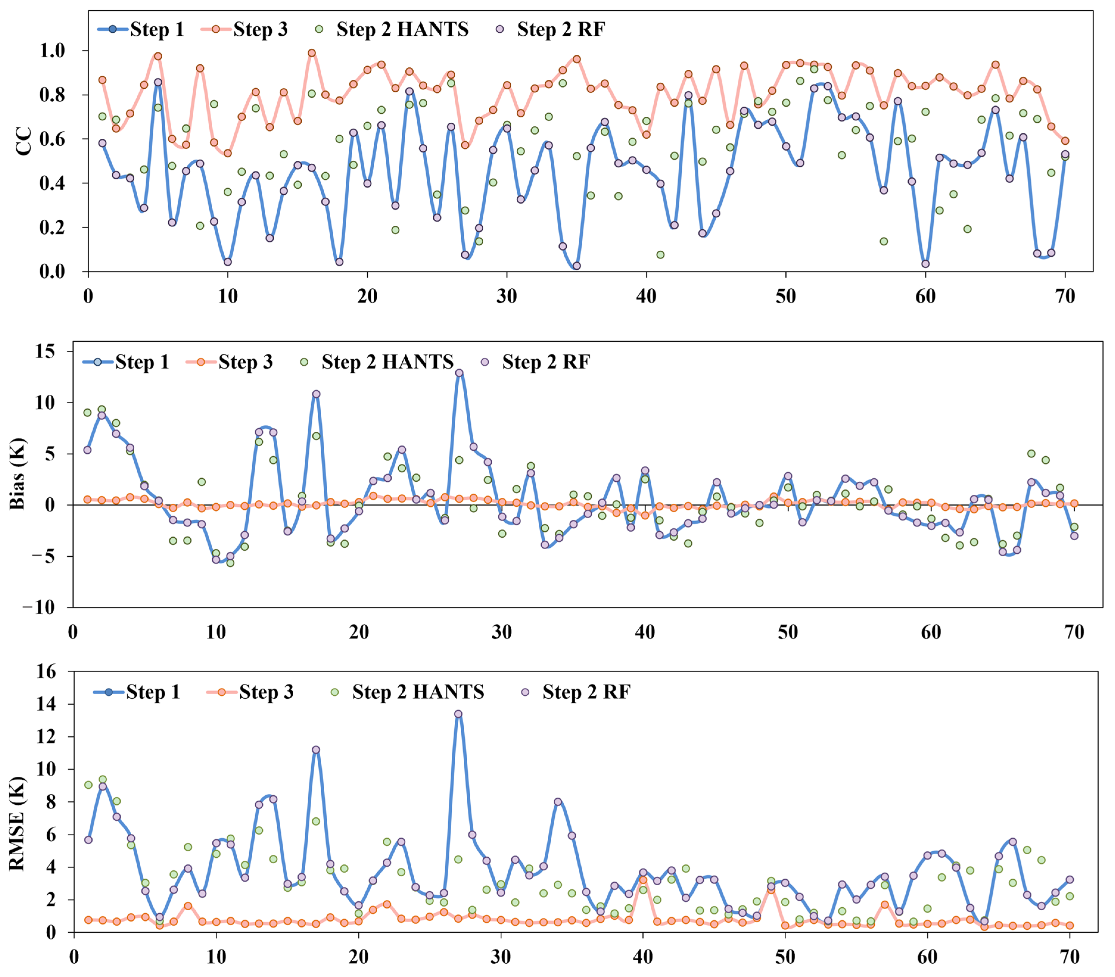
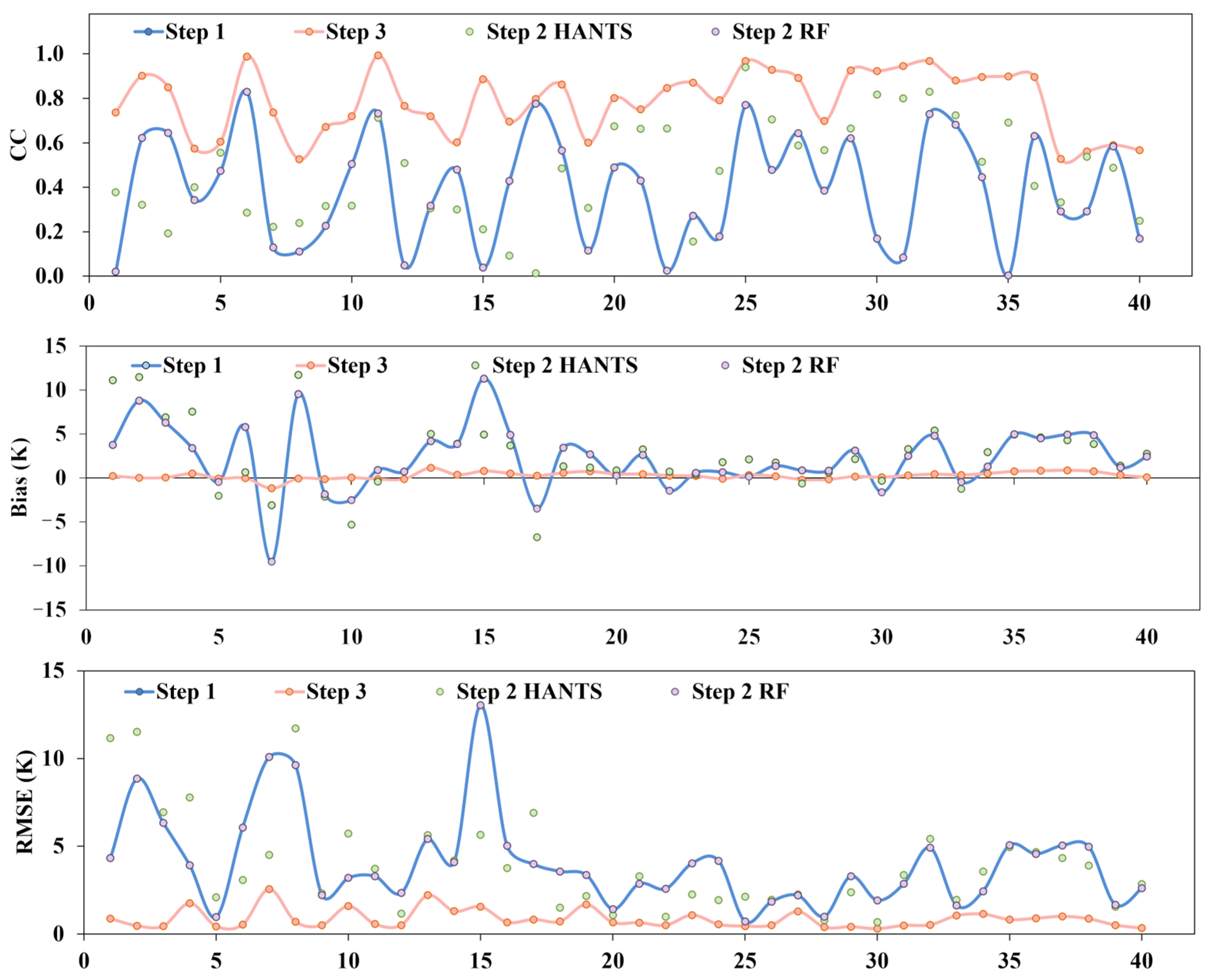
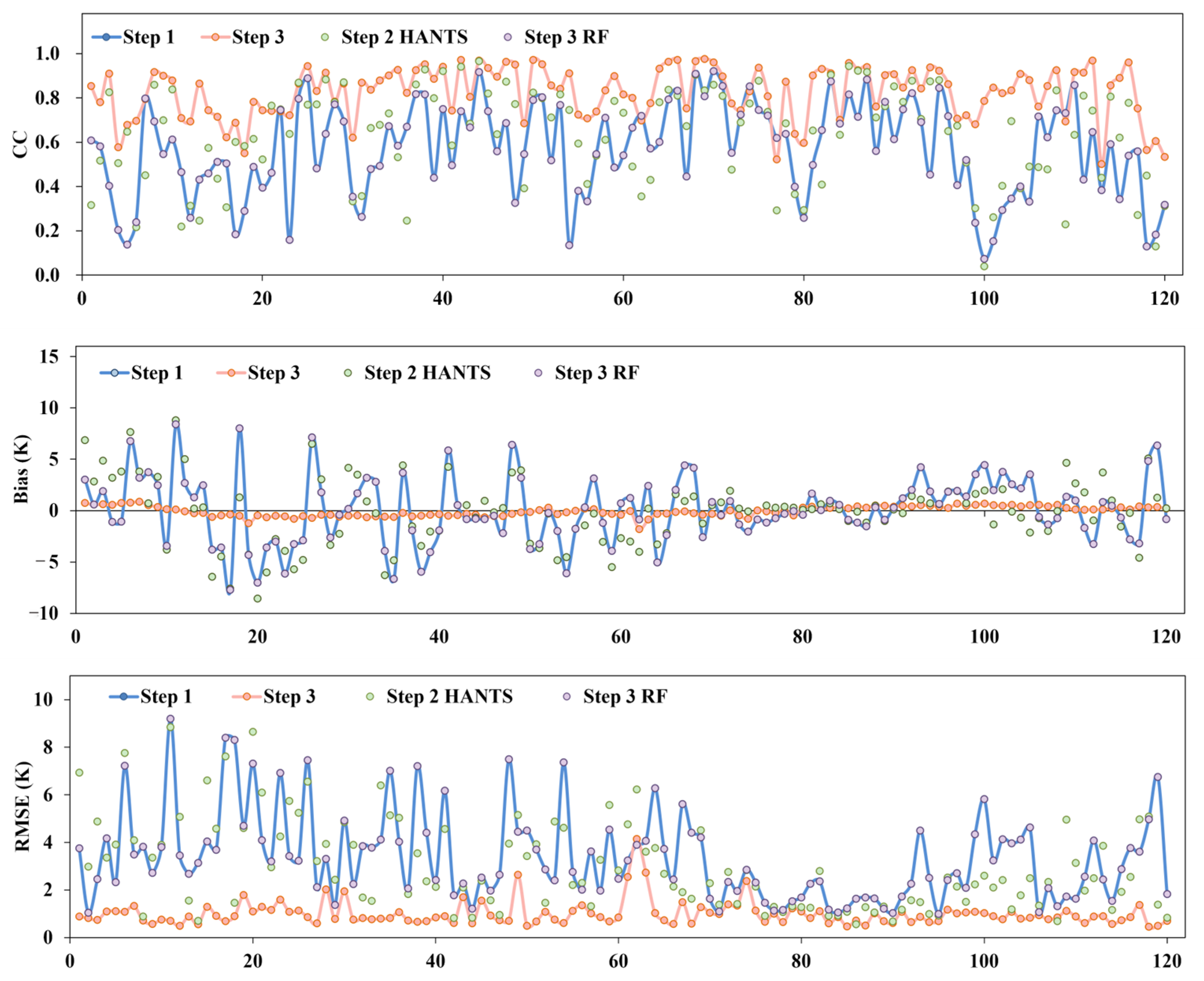
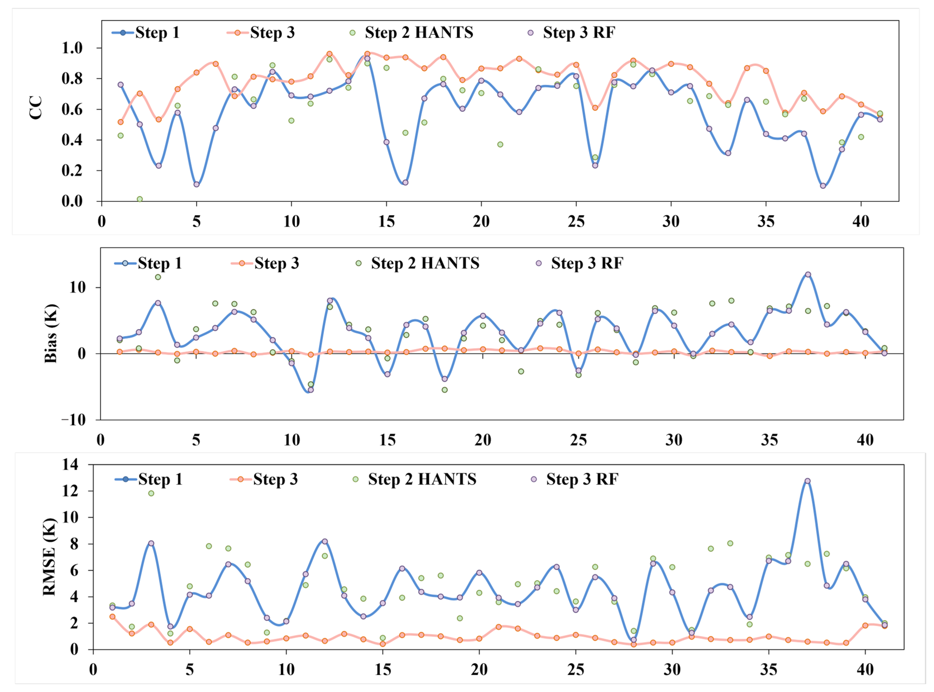
This study conducted a systematic quantitative evaluation of reconstruction accuracy for LST under clear-sky conditions. A large number of daily MODIS LST images from two representative regions—Huainan and Jining—were selected, covering both daytime and nighttime periods. In each image, multiple simulated missing patterns were created by masking pixels at varying proportions, representing diverse gap scenarios. A multi-stage integrated reconstruction framework was applied sequentially, including the following: (1) Step 1: initial gap filling based on background information; (2) Step 2: HANTS and RF, representing interannual time-series interpolation and multivariate modeling, respectively; and (3) Step 3: the final integrated reconstruction, combining the strengths of previous stages. The reconstruction results at each step were compared against the original pixel values using three key metrics: correlation coefficient (CC), Bias (K), and root mean square error (RMSE, K). Detailed results are shown in Figure 14, Figure 15, Figure 16 and Figure 17 and

Table 5. Statistical evaluation of reconstruction accuracy for missing pixels in selected daytime LST images.

Day	HN (71 Images)			JN (121 Images)
	CC	Bias (K)	RMSE (K)	CC	Bias (K)	RMSE (K)
Step 1	0.900	0.714	4.448	0.886	2.310	5.003
Step 2 HANTS	0.937	0.901	3.967	0.901	2.584	5.088
Step 2 RF	0.902	0.701	4.389	0.887	2.270	5.053
Step 3	0.996	0.147	0.861	0.995	0.251	1.021

and

Table 6. Overall quantitative evaluation of missing pixel reconstruction in selected nighttime images.

Night	HN (40 Images)			JN (41 Images)
	CC	Bias (K)	RMSE (K)	CC	Bias (K)	RMSE (K)
Step 1	0.886	2.310	5.003	0.908	3.023	5.194
Step 2 HANTS	0.901	2.584	5.088	0.908	3.206	5.327
Step 2 RF	0.898	2.230	4.998	0.907	3.018	5.104
Step 3	0.995	0.251	1.021	0.994	0.274	1.155

.

For daytime LST images, a total of 71 (Huainan) and 121 (Jining) simulated missing samples were evaluated. As seen in Figure 14 and Figure 16, reconstruction accuracy improves significantly as the process advances. Step 1, being an initial approximation, performs poorly overall—CC typically remains at a low level between 0.4 and 0.6, with sharp drops on several dates. Bias can reach ±10 K, and RMSE peaks near 14 K, indicating substantial reconstruction errors. In contrast, Step 3 maintains CC values consistently above 0.85, with most cases exceeding 0.95. Bias remains within ±2 K, and RMSE is generally below 2 K, reflecting excellent consistency and robustness. Although Step 2 HANTS and Step 2 RF occasionally improve performance, they still suffer from issues such as large biases or detail loss, and fail to match the quality of the final integrated result.

The statistical summary in Table 5 further supports this trend. Taking the Huainan region as an example, Step 3 achieves a CC of 0.996—significantly better than Step 1 (0.900), Step 2 HANTS (0.937), and Step 2 RF (0.902). Its Bias and RMSE are only 0.147 K and 0.861 K, respectively, whereas Step 1 shows much higher errors at 0.714 K (Bias) and 4.448 K (RMSE). The Jining region exhibits a similar pattern: Step 3 yields an RMSE of just 1.021 K, while HANTS exceeds 5 K—nearly five times larger—demonstrating Step 3’s strong generalization ability across multiple images and large spatial scales.

Moreover, the scatter plots in Figure 18 and Figure 19 further validate the reconstruction consistency of each method. Pixel values reconstructed by Step 3 are highly concentrated along the 1:1 diagonal, with the regression slope close to 1 and a coefficient of determination (R²) of 0.991, indicating minimal error and excellent spatial agreement. In contrast, the point clouds from Step 1 and HANTS are visibly dispersed and deviate significantly from the ideal line, revealing evident systematic biases and error stretching artifacts.

In nighttime LST reconstruction tasks (see Figure 15 and Figure 17 and Table 6), the inherently weaker surface temperature signals and stronger atmospheric interference make the reconstruction process more challenging and prone to amplified errors. Nevertheless, even under such complex conditions, Step 3, as the final stage of the integrated reconstruction framework, demonstrates clear and significant advantages.

As shown in Figure 15 and Figure 17, both Step 1 and Step 2 HANTS exhibit considerable volatility across many nighttime images: Bias values can reach up to ±12 K, and RMSE exceeds 10 K in certain cases, indicating that reconstruction errors are substantially amplified under low signal-to-noise conditions. For instance, between the 10th and 20th images in the Huainan dataset, HANTS results fluctuate dramatically, showing poor stability. In contrast, Step 3 delivers markedly more stable reconstructions, with both Bias and RMSE consistently remaining at low levels and exhibiting minimal fluctuation, without notable outliers. The CC values for Step 3 are stably maintained within the 0.95–0.99 range, significantly higher than the 0.7–0.9 range observed for Step 1 and HANTS, indicating superior consistency and reliability.

The statistics in Table 6 further validate these observations. For the nighttime data in Huainan, Step 3 achieves a CC of 0.995, a Bias of 0.251 K, and an RMSE of 1.021 K—substantially outperforming Step 1 (CC = 0.886, Bias = 2.310 K, RMSE = 5.003 K) and HANTS (RMSE = 5.088 K). In the Jining region, Step 3 also shows the best performance, with an RMSE of just 1.155 K, compared to 5.327 K for HANTS and 5.194 K for Step 1—more than four times higher. These results highlight the strong adaptability and robustness of Step 3’s optimization-based integration mechanism, even under challenging nighttime conditions.

Scatter plots in Figure 20 and Figure 21 provide additional confirmation. The pixel values reconstructed by Step 3 closely match the original values, with scatter points densely aligned along the 1:1 reference line. The linear fit slope is nearly 1, and the coefficient of determination (R²) exceeds 0.99 in both cases, reflecting dual advantages in spatial consistency and numerical accuracy. By contrast, the reconstructions from HANTS and Step 1 are more dispersed, with more outliers and clear systematic deviations from the reference line, resulting in reduced overall fit quality.

Taken together, the daytime and nighttime quantitative evaluations confirm that Step 3 is not merely a single algorithm, but rather a hybrid strategy that combines spatial constraints, temporal modeling, and residual correction. It progressively suppresses errors and enhances consistency across all reconstruction stages. Whether under high-temperature gradients during the day or weak-signal conditions at night, Step 3 consistently outperforms other methods in terms of correlation, error control, and stability.

Especially in nighttime scenarios—which are inherently more difficult—Step 3’s superior accuracy and robustness underscore its broad applicability and strong generalization capability. Therefore, it can be considered a preferred solution for large-scale, multi-temporal MODIS LST gap-filling tasks, outperforming conventional methods such as pure temporal interpolation (e.g., HANTS) and spatial averaging approaches.

4.3. Visual Spatial Validation of MODIS Reconstruction Against Landsat LST

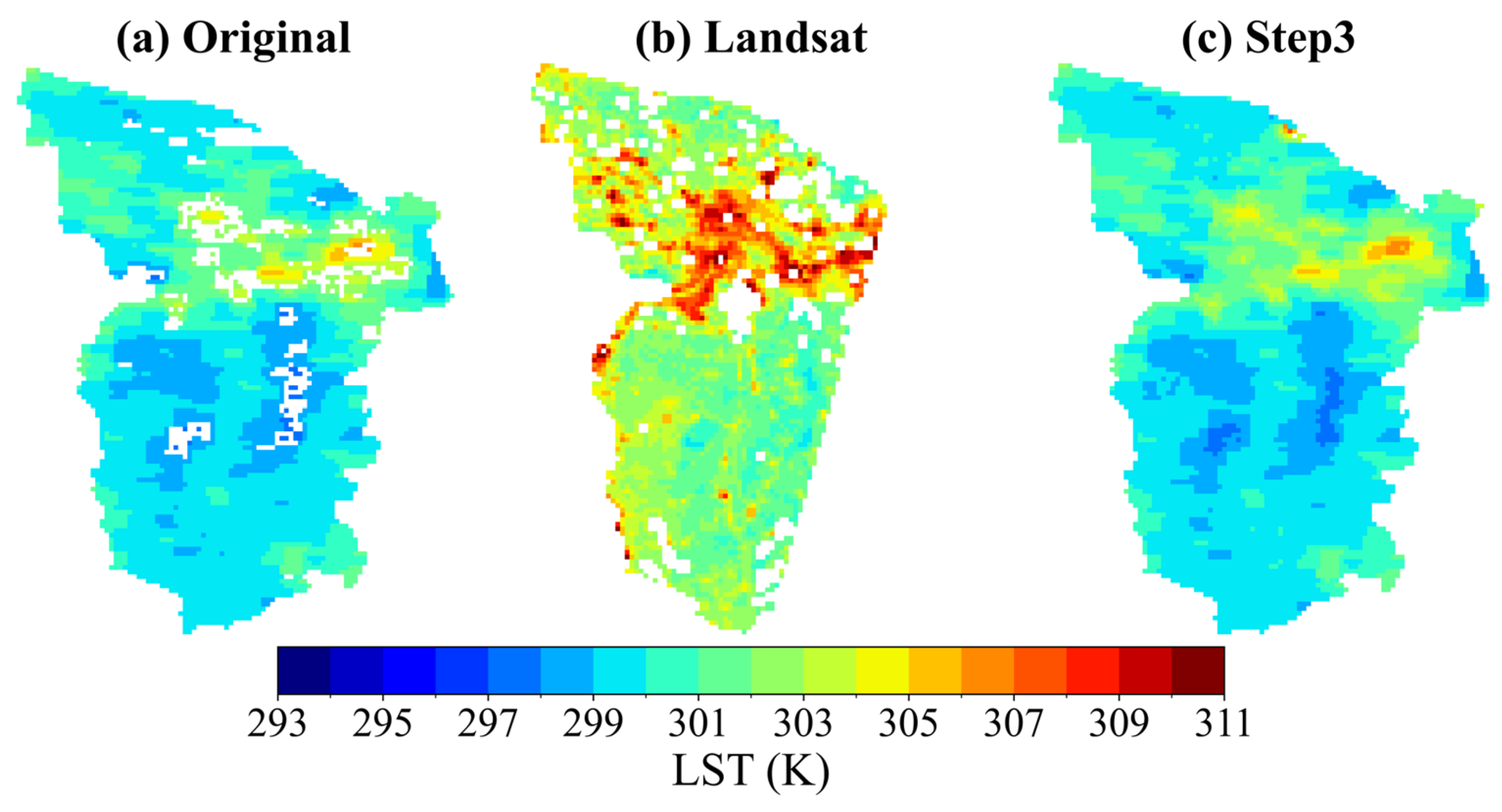
To further validate the spatial adaptability and cross-scale accuracy of the proposed Step 3 integrated reconstruction method, two representative daytime scenes from the Huainan and Jining regions (acquired on 8 September and 23 August 2018, respectively) were selected for analysis. Landsat LST data were used as a reference to visually and quantitatively compare the original MODIS LST, the Step 3 reconstruction results, and the Landsat LST, as illustrated in Figure 22 and Figure 23 and summarized in

Table 7. Quantitative evaluation of MODIS and reconstructed LST against Landsat reference for two selected images.

* vs. Landsat	HN (8 September 2018)			JN (23 September 2018)
	CC	Bias	RMSE	CC	Bias	RMSE
Modis	0.765	−3.015	3.203	0.720	−2.792	3.013
Reconstructed	0.751	−2.465	2.657	0.822	−1.920	2.100

* denotes MODIS LST and reconstructed LST.

.

From the spatial distribution maps in Figure 22 and Figure 23, it is evident that the original MODIS LST images (Panel a) provide broad regional coverage but suffer from extensive missing areas due to cloud contamination or other quality-related issues. These gaps are particularly prominent in regions with sparse vegetation or complex terrain. Landsat LST images (Panel b), with their higher spatial resolution, are capable of capturing fine-scale thermal anomalies but are limited in coverage, making them unsuitable for large-scale continuous monitoring.

The Step 3 reconstruction results (Panel c) effectively retain the wide-area coverage of MODIS while significantly enhancing spatial continuity and the recovery of local thermal details. In the Huainan scene (Figure 22), the reconstructed LST appears smoother and it aligns well with high-temperature zones observed in the Landsat imagery—for example, in the central urban area and northern bare land, where thermal hotspots are clearly restored. Similarly, in the Jining scene (Figure 23), Step 3 successfully captures the temperature gradient structures evident in the Landsat image, particularly in transitional zones around the urban edge and agricultural areas. The boundaries between hot and cool zones become more distinct, mitigating the spatial discontinuities caused by missing data in the original MODIS images.

Quantitative analysis further confirms the advantages of Step 3 in restoring spatial details. As shown in Table 7, the reconstruction results yield lower RMSE and Bias values when compared against Landsat LST in both regions, indicating that Step 3 effectively reduces both systematic and absolute errors relative to the original MODIS data. In the Huainan region, RMSE decreased from 3.203 K (MODIS) to 2.657 K, and Bias reduced from –3.015 K to –2.465 K, showing a marked improvement. In Jining, the performance was even more notable: the correlation coefficient (CC) increased from 0.720 to 0.822, and RMSE dropped from 3.013 K to 2.100 K. These results demonstrate that Step 3 not only improves consistency with Landsat data but also significantly enhances the spatial accuracy of temperature estimation.

In summary, the Step 3 integrated reconstruction method exhibits excellent cross-scale adaptability. It preserves the spatiotemporal characteristics of MODIS while incorporating Landsat-level spatial detail, enabling high-accuracy reconstruction of large-scale LST data. This approach provides a feasible pathway for applying MODIS LST to high-resolution applications and shows strong potential for broader adoption in studies of surface processes in thermally sensitive areas such as urban heat islands and energy development zones.

4.4. Quantitative Error Validation Through Comparison with Landsat LST

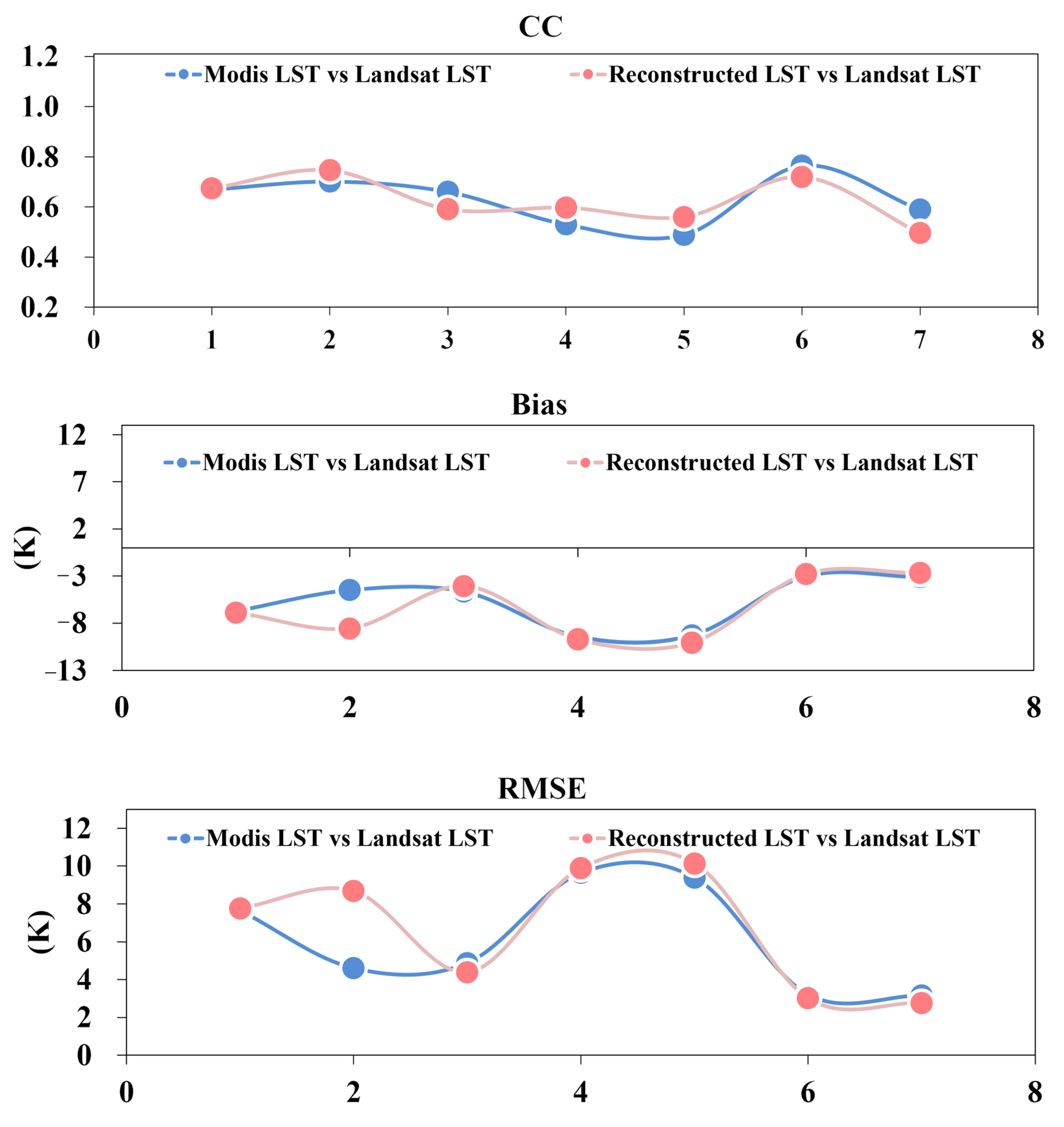
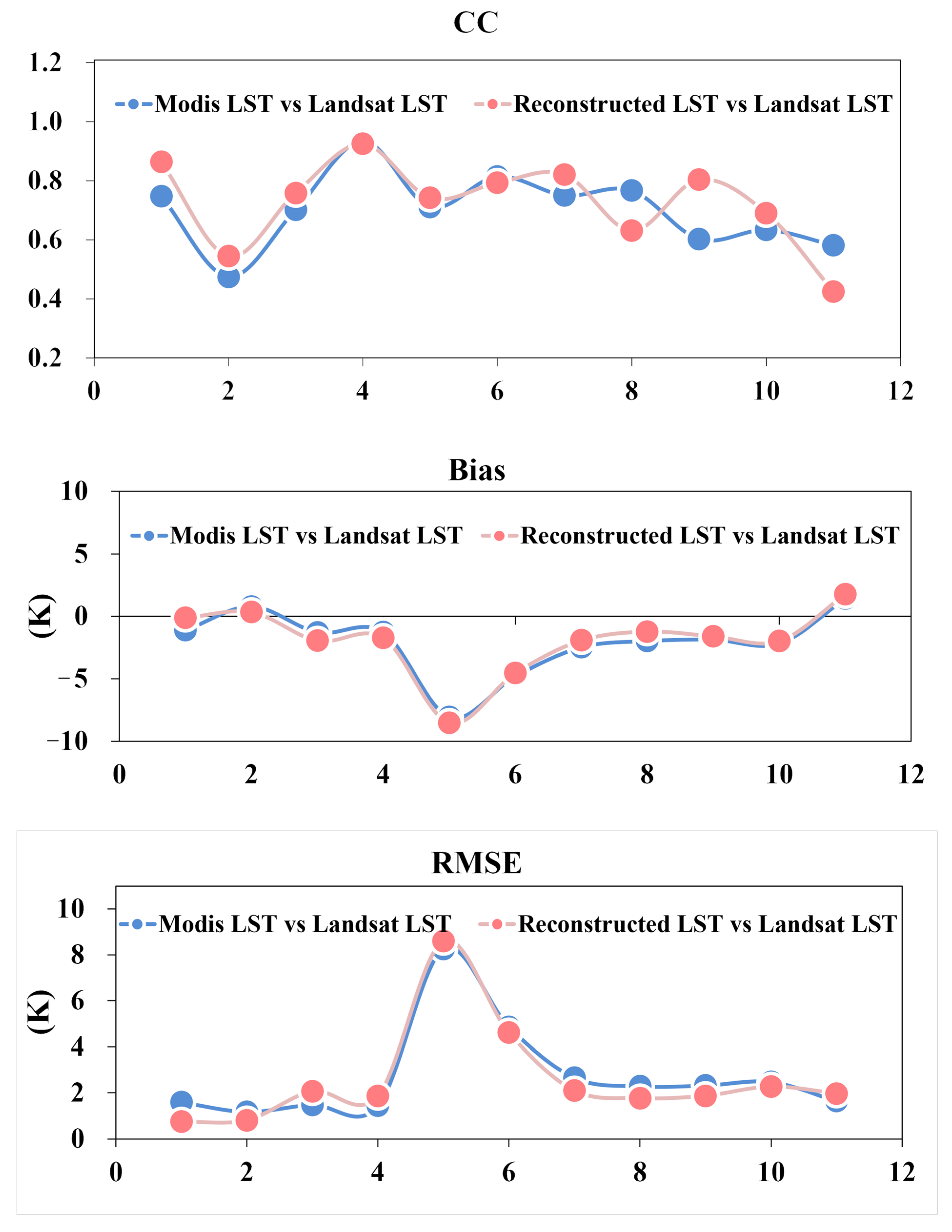
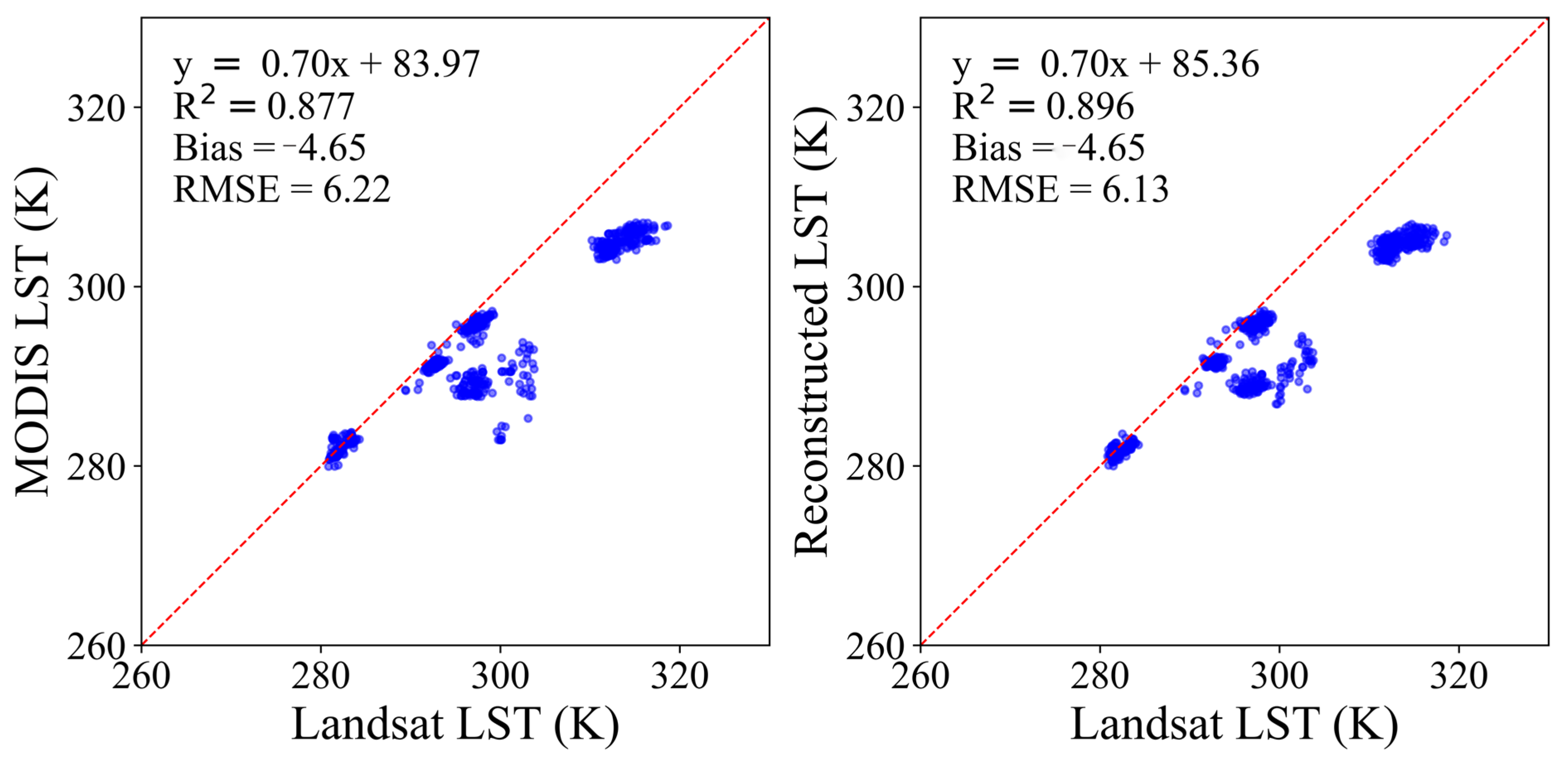
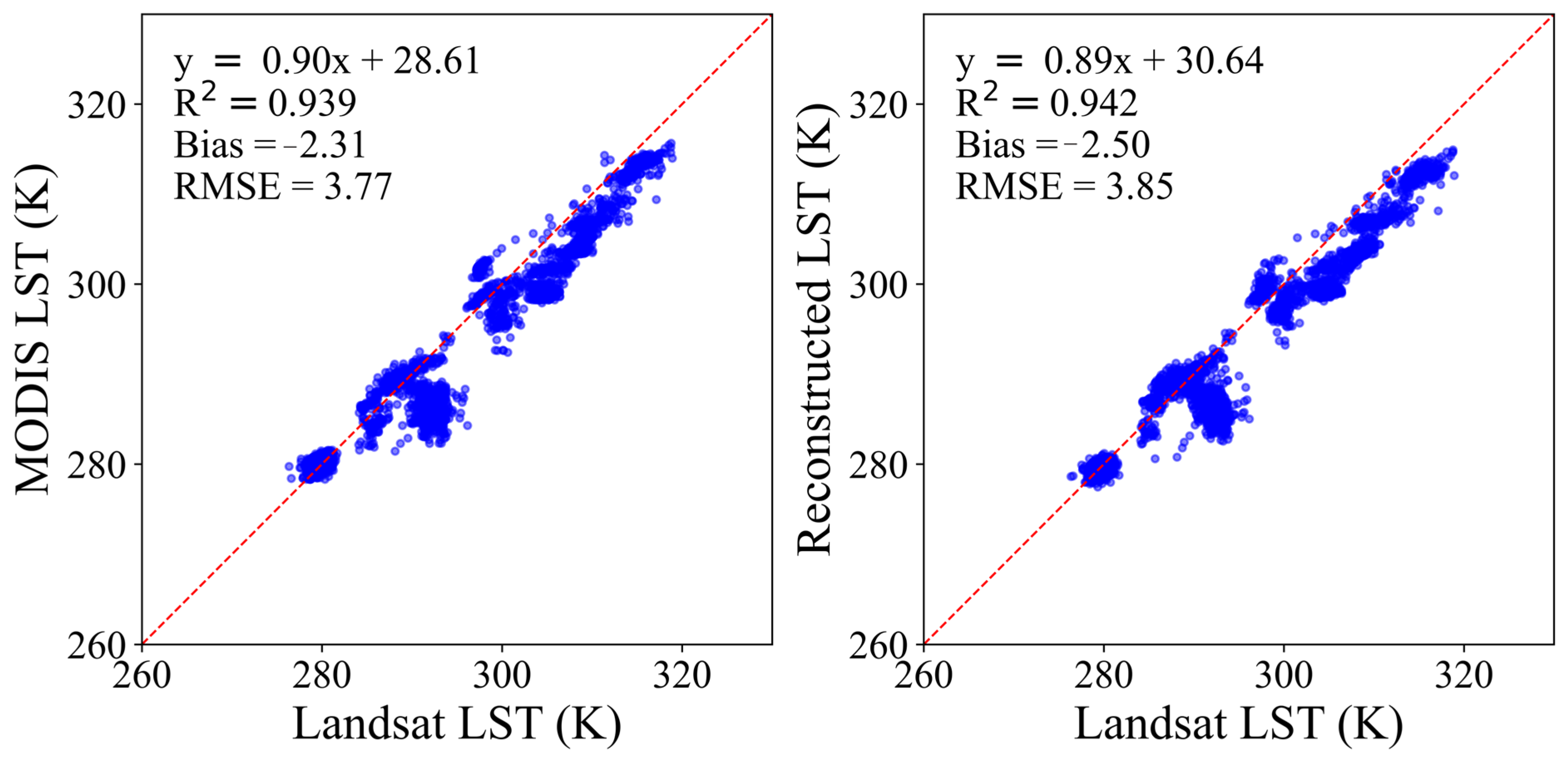
Based on the results shown in Figure 24, Figure 25, Figure 26 and Figure 27 and

Table 8. Overall quantitative evaluation of missing pixel reconstruction in selected images (36 images in Huainan and 64 in Jining during 2018, with 7 and 11 matched with Landsat, respectively; ~50% match rate).

* vs. Landsat	HN (7 Images)			JN (11 Images)
	CC	Bias (K)	RMSE (K)	CC	Bias (K)	RMSE (K)
Modis	0.867	−5.988	7.159	0.981	−1.828	3.052
Reconstructed	0.846	−5.950	7.275	0.984	−1.677	2.978

* denotes MODIS LST and reconstructed LST.

, a further quantitative validation was conducted using Landsat LST as a high-resolution reference to assess the spatial consistency and accuracy of both the original MODIS LST and the Step 3-reconstructed values.

In Figure 24 and Figure 25, seven images from each of the Huainan and Jining regions were selected, and three key evaluation metrics—correlation coefficient (CC), Bias, and RMSE—were compared across scenes. Overall, the Step 3-reconstructed LST shows comparable or even better correlation with Landsat LST than the original MODIS data in most cases. For instance, in the Huainan region (Figure 24), CC values for both datasets remain generally stable between 0.6 and 0.8, with a consistent trend. Step 3 also tends to yield slightly lower Bias in many scenes, suggesting improved deviation control. In terms of RMSE, the Step 3 curve falls below that of MODIS in several instances, with errors reduced by more than 0.5 K in scenes 3 and 5. In the Jining region (Figure 25), the improvement is more evident: Step 3 achieves higher CC values in many images, with a peak close to 0.95. Both Bias and RMSE are also consistently lower than those of MODIS, especially in scenes 6 through 10, where error control is significantly enhanced.

Table 8 summarizes the quantitative results for all missing pixels across the seven Huainan and eleven Jining scenes. The findings further confirm that the reconstruction accuracy of Step 3 does not deteriorate compared to original MODIS values; in fact, some metrics even show improvements. For example, in the Jining region, the CC between reconstructed LST and Landsat reaches 0.984, slightly higher than 0.981 for MODIS; Bias is reduced to –1.68 K and RMSE is reduced to 2.978 K, both lower than the MODIS values (Bias = –1.83 K; RMSE = 3.052 K). In the Huainan region, performance is slightly lower but still comparable: the reconstructed CC is 0.846 versus 0.867 for MODIS, but Bias improves from –5.988 K to –5.950 K, and RMSE remains around 7.3 K.

Scatter plots in Figure 26 and Figure 27 further support these findings at the pixel level. In the comparison between MODIS LST and Landsat, the scatter distributions are relatively dispersed, with regression lines deviating from the ideal 1:1 reference line. The slope is approximately 0.70–0.81, and R² values are 0.877 (HN) and 0.963 (JN). By contrast, Step 3 reconstructions show slightly improved regression slope and intercepts; in Jining, R² increases to 0.967, and both Bias and RMSE are reduced. These results suggest that the Step 3 integrated method produces reconstructions that are more spatially consistent with Landsat observations and exhibit higher physical plausibility and adaptability.

In summary, this comparison indicates that although MODIS LST inherently suffers from lower spatial resolution and certain systematic biases, the Step 3 integrated reconstruction method can significantly enhance spatial consistency and accuracy while retaining the strong temporal coverage of MODIS. This makes Step 3 a highly applicable and scalable solution for high-precision LST analysis, especially in applications requiring reliable spatial detail.

5. Discussion

The multi-stage integrated reconstruction method proposed in this study demonstrates excellent adaptability and accuracy for clear-sky MODIS LST reconstruction. Both simulated missing-data experiments and comparisons with in situ high-resolution references confirm that the proposed approach exhibits strong spatial consistency across large-scale regions and significantly outperforms the conventional HANTS method and the original MODIS LST product in error control. Particularly in the Step 3 integration phase, the method effectively combines the spatial constraint of Step 1, the temporal continuity of Step 2 HANTS, and the multivariate learning capability of Step 2 RF, enabling high-quality reconstruction of missing pixels while preserving both spatial structure and physical process consistency.

Quantitative results (Figure 14, Figure 15, Figure 16 and Figure 17, Table 6 and Table 7) show that Step 3 maintains RMSE within 2 K and correlation coefficients (CCs) generally above 0.95 under both daytime and nighttime conditions. The scatter plot analyses (Figure 18, Figure 19, Figure 20 and Figure 21) further reveal that reconstructed values are densely clustered along the 1:1 reference line, indicating high pixel-level agreement. However, certain reconstruction errors remain under specific conditions or in particular regions, which can be attributed to the following factors:

(1) Model errors and feature representation limitations

The Step 2 RF and Step 3 phases incorporate multiple remote sensing features (e.g., NDVI, NDWI, DEM, land cover, and LST time series). However, the nonlinear relationships between these variables and LST can vary by region and temporal phase, making them difficult to fully capture. This is especially evident in mining areas and urban fringes, where the correlation between vegetation indices and surface temperature weakens. In such cases, the random forest model may overfit during training, leading to artifacts such as anomalous hotspots or blurred boundaries. In addition, Land Surface Temperature is also significantly influenced by temporal and radiative driving factors such as day of year (DOY) and solar radiation, which were not explicitly incorporated into the current framework. Although the multi-year daily mean LST partly reflects DOY and seasonal patterns, and MODIS reflectance can indirectly characterize radiative properties, future studies should consider integrating DOY, total solar radiation, or meteorological reanalysis data (e.g., ERA5) to enhance the temporal consistency and physical rationality of the reconstruction results.

(2) Error propagation from the spatial interpolation stage

The initial interpolation (Step 1) uses a neighborhood mean constrained by land cover and elevation, which is efficient for filling small gaps in homogeneous areas. However, in heterogeneous environments such as mountainous regions, river valleys, or urban–rural transition zones, this method cannot ensure structural continuity and may cause boundary discontinuities or banding artifacts (see Region 2 and Region 3 in Figure 10, Figure 11, Figure 12 and Figure 13). These structural errors can be learned and retained by subsequent modeling, resulting in systematic biases in the final output.

(3) Smoothing bias in temporal reconstruction

Although HANTS is robust for capturing seasonal LST patterns and suitable for large-scale, long-term gap filling, its inherent smoothing mechanism can suppress extreme temperature events or rapid fluctuations. This limitation is especially apparent in summer or in high-disturbance areas such as mining zones (e.g., Region 3 in Figure 13). In such cases, although Step 2 HANTS may achieve high CC values, it still exhibits relatively high Bias and RMSE, indicating a weakness in detecting anomalies and short-term variability.

(4) Source data errors and edge pixel effects

Despite rigorous filtering of MODIS QA = 00 pixels for training and reconstruction, and application of morphological erosion at image boundaries, the accuracy of MODIS QA flags in detecting cloud shadows, bright surfaces, or high-humidity regions remains limited. Some low-quality pixels may be mistakenly retained, leading to biased model learning and over- or underestimation of LST. Additionally, auxiliary variables such as NDVI or land cover may contain classification errors or temporal mismatches, thereby introducing noise and affecting model stability in localized areas.

(5) Resolution effects

The spatial resolution of MODIS LST is only 1 km, which tends to enhance pixel-level consistency over large-scale regions. As a result, the R² values reported in this study may be somewhat inflated, while RMSE may be underestimated. Although comparison with Landsat LST demonstrates that the proposed method performs well in terms of spatial consistency and error control, its applicability and robustness at higher resolutions (e.g., Sentinel-3, Landsat, ECOSTRESS) still require further investigation.

(6) Validation limitations

The validation in this study mainly relied on MODIS internal QA high-quality pixels and cross-comparisons with Landsat LST. While this provides useful reference information, direct support from ground-based observations is still lacking. Even in the absence of such data, this limitation should be explicitly acknowledged. Future research could benefit from incorporating meteorological station observations or ground-based radiometer measurements, which would provide stronger constraints on the reconstruction results and significantly enhance their credibility and application value.

In summary, the proposed multi-stage integrated reconstruction strategy demonstrates significant advantages in terms of spatial consistency, temporal continuity, and error suppression. It maintains high accuracy and robustness even under complex scenarios such as diurnal alternation and strong regional heterogeneity. Nevertheless, future studies should address the above limitations, particularly by incorporating additional temporal and radiative driving factors, testing at higher spatial resolutions, and conducting multi-source validation with ground-based observations, in order to further enhance the physical consistency, transferability, and application potential of this approach for large-scale MODIS LST reconstruction tasks.

6. Conclusions

This study addresses the problem of missing value reconstruction in clear-sky MODIS LST data by proposing a multi-stage integrated method that combines spatial structural constraints, temporal fitting, and multivariate modeling. Based on extensive simulated and real remote sensing imagery from two representative regions—Huainan and Jining—the reconstruction accuracy, stability, and spatial adaptability of the proposed approach were systematically evaluated. The main conclusions are as follows:

The multi-stage integrated method significantly improves LST reconstruction accuracy and stability. The proposed Step 3 fusion strategy effectively combines the neighborhood-based spatial information from Step 1, the temporal continuity of Step 2 HANTS, and the multivariate feature learning of Step 2 RF. This integration suppresses the respective limitations of individual methods. In simulated missing data experiments, the method consistently achieved high correlation and low reconstruction error, with RMSE generally below 2 K and CC exceeding 0.95 for both daytime and nighttime scenes. Overall performance clearly surpasses that of HANTS and the original MODIS product, demonstrating strong robustness and generalization capability.

The method remains effective under complex missing patterns and low signal-to-noise conditions. Even under challenging scenarios such as nighttime scenes with weak thermal signals and high spatial heterogeneity, Step 3 maintains stable reconstruction output. It effectively reduces boundary artifacts present in Step 1 and suppresses over-smoothing effects from HANTS. The RMSE and Bias are significantly reduced, and issues such as local anomalies or discontinuities are avoided. These results indicate the method’s applicability to a wide range of complex remote sensing reconstruction tasks.

Cross-scale validation confirms Step 3’s adaptability to high-resolution spatial features. Spatial comparisons with Landsat LST demonstrate that Step 3 not only outperforms the original MODIS data in terms of RMSE and Bias, but also better restores medium-to-high temperature areas and boundary structures. Correlation analysis and pixel-level scatter plots further verify its dual advantages in spatial consistency and physical realism, making it well-suited for LST studies that require a balance between spatial coverage and estimation accuracy.

References

1. Yan, J.; Chen, H.; Wu, H.; Wang, N.; Ma, L. A Method for Estimating 1 Km All-Weather Hourly Land Surface Temperature. In Proceedings of the 2022 IEEE International Geoscience and Remote Sensing Symposium (IGARSS 2022), Kuala Lumpur, Malaysia, 17–22 July 2022; IEEE: New York, NY, USA, 2022; pp. 3664–3667. [Google Scholar]
2. Wang, M.; He, C.; Zhang, Z.; Hu, T.; Duan, S.-B.; Mallick, K.; Li, H.; Liu, X. Evaluation of Three Land Surface Temperature Products from Landsat Series Using in Situ Measurements. IEEE Trans. Geosci. Remote Sens. 2023, 61, 5000119. [Google Scholar] [CrossRef]
3. Han, X.-J.; Tang, H.; Lie, Z.-L.; Duan, S.-B.; Wu, Y.; Leng, P.; Chen, X. Retrieval of Land Surface Temperature and Soil Moisture from Passive Microwave Observations. In Proceedings of the 2021 IEEE International Geoscience and Remote Sensing Symposium Igarss, Brussels, Belgium, 11–16 July 2021; IEEE: New York, NY, USA, 2021; pp. 6190–6193. [Google Scholar]
4. Meng, X.; Cheng, J.; Guo, H.; Guo, Y.; Yao, B. Accuracy Evaluation of the Landsat 9 Land Surface Temperature Product. IEEE J. Sel. Top. Appl. Earth Observ. Remote Sens. 2022, 15, 8694–8703. [Google Scholar] [CrossRef]
5. Pan, Y.; Gao, Y.; Li, S. Impacts of Land Use/Land Cover Distributions and Vegetation Amount on Land Surface Temperature Simulation in East China. Earth Space Sci. 2021, 8, e2020EA001544. [Google Scholar] [CrossRef]
6. Nega, W.; Balew, A. The Relationship between Land Use Land Cover and Land Surface Temperature Using Remote Sensing: Systematic Reviews of Studies Globally over the Past 5 Years. Environ. Sci. Pollut. Res. 2022, 29, 42493–42508. [Google Scholar] [CrossRef] [PubMed]
7. Al Shawabkeh, R.; AlHaddad, M.; Al-Fugara, A.; Al-Hawwari, L.; Al-Hawwari, M.I.; Omoush, A.; Arar, M. Modeling the Impact of Urban Land Cover Features and Changes on the Land Surface Temperature (LST): The Case of Jordan. Ain Shams Eng. J. 2024, 15, 102359. [Google Scholar] [CrossRef]
8. Du, W.; Li, Z.-L.; Qin, Z.; Fan, J.; Liu, X.; Zhao, C.; Cao, K. Reconstruction of Cloudy Land Surface Temperature by Combining Surface Energy Balance Theory and Solar-Cloud-Satellite Geometry. IEEE Trans. Geosci. Remote Sens. 2025, 63, 5001513. [Google Scholar] [CrossRef]
9. Li, Y.; He, Q.; Liu, Y.; Yan, Y.; Zhang, H.; Tan, J. A Physically Constrained Downscaling Framework for Hourly, All-Sky Land Surface Temperature in Mountainous Regions. IEEE J. Sel. Top. Appl. Earth Observ. Remote Sens. 2025, 18, 8151–8174. [Google Scholar] [CrossRef]
10. Zhang, X.; Zhou, J.; Dong, W.; Song, L. Estimation of 1-Km All-Weather Land Surface Temperature Over the Tibetan Plateau. In Proceedings of the IGARSS 2018—2018 IEEE International Geoscience and Remote Sensing Symposium, Valencia, Spain, 22–27 July 2018; IEEE: New York, NY, USA, 2018; pp. 3430–3433. [Google Scholar]
11. Nguyen, O.V.; Kawamura, K.; Dung, P.T.; Gong, Z.; Suwandana, E. Temporal Change and Its Spatial Variety on Land Surface Temperature and Land Use Changes in the Red River Delta, Vietnam, Using MODIS Time-Series Imagery. Environ. Monit. Assess. 2015, 187, 464. [Google Scholar] [CrossRef]
12. Wan, Z.M.; Zhang, Y.L.; Zhan, Q.C.; Li, Z.L. The MODIS Land-Surface Temperature Products for Regional Environmental Monitoring and Global Change Studies. In Proceedings of the IGARSS 2002: IEEE International Geoscience and Remote Sensing Symposium and 24th Canadian Symposium On Remote Sensing, Vols I-Vi, Proceedings: Remote Sensing: Integrating Our View Of The Planet, Toronto, ON, Canada, 24–28 June 2002; IEEE: New York, NY, USA, 2002; pp. 3683–3685. [Google Scholar]
13. Wang, J.; Tang, R.; Jiang, Y.; Liu, M.; Li, Z.-L. A Practical Method for Angular Normalization of Global MODIS Land Surface Temperature over Vegetated Surfaces. ISPRS-J. Photogramm. Remote Sens. 2023, 199, 289–304. [Google Scholar] [CrossRef]
14. Long, D.; Yan, L.; Bai, L.; Zhang, C.; Li, X.; Lei, H.; Yang, H.; Tian, F.; Zeng, C.; Meng, X.; et al. Generation of MODIS-like Land Surface Temperatures under All-Weather Conditions Based on a Data Fusion Approach. Remote Sens. Environ. 2020, 246, 111863. [Google Scholar] [CrossRef]
15. Wang, Z.; Yang, Y.; Hu, P.; Dai, Y.; Meng, X. A Hybrid Method for Temporal Normalization of Land Surface Temperature Under All-Sky Conditions. IEEE J. Sel. Top. Appl. Earth Observ. Remote Sens. 2024, 17, 16139–16153. [Google Scholar] [CrossRef]
16. Yang, G.; Sun, W.; Shen, H.; Meng, X.; Li, J. An Integrated Method for Reconstructing Daily MODIS Land Surface Temperature Data. IEEE J. Sel. Top. Appl. Earth Obs. Remote Sens. 2019, 12, 1026–1040. [Google Scholar] [CrossRef]
17. Duan, S.-B.; Han, X.-J.; Huang, C.; Li, Z.-L.; Wu, H.; Qian, Y.; Gao, M.; Leng, P. Land Surface Temperature Retrieval from Passive Microwave Satellite Observations: State-of-the-Art and Future Directions. Remote Sens. 2020, 12, 2573. [Google Scholar] [CrossRef]
18. Zhao, W.; Duan, S.-B. Reconstruction of Daytime Land Surface Temperatures under Cloud-Covered Conditions Using Integrated MODIS/Terra Land Products and MSG Geostationary Satellite Data. Remote Sens. Environ. 2020, 247, 111931. [Google Scholar] [CrossRef]
19. Yu, Y.; Renzullo, L.J.; McVicar, T.R.; Malone, B.P.; Tian, S. Generating Daily 100 m Resolution Land Surface Temperature Estimates Continentally Using an Unbiased Spatiotemporal Fusion Approach. Remote Sens. Environ. 2023, 297, 113784. [Google Scholar] [CrossRef]
20. Li, B.; Liang, S.; Ma, H.; Dong, G.; Liu, X.; He, T.; Zhang, Y. Generation of Global 1 km All-Weather Instantaneous and Daily Mean Land Surface Temperatures from MODIS Data. Earth Syst. Sci. Data 2024, 16, 3795–3819. [Google Scholar] [CrossRef]
21. Fu, P.; Xie, Y.; Weng, Q.; Myint, S.; Meacham-Hensold, K.; Bernacchi, C. A Physical Model-Based Method for Retrieving Urban Land Surface Temperatures under Cloudy Conditions. Remote Sens. Environ. 2019, 230, 111191. [Google Scholar] [CrossRef]
22. Jin, M.L. Interpolation of Surface Radiative Temperature Measured from Polar Orbiting Satellites to a Diurnal Cycle 2. Cloudy-Pixel Treatment. J. Geophys. Res.-Atmos. 2000, 105, 4061–4076. [Google Scholar] [CrossRef]
23. Shiff, S.; Helman, D.; Lensky, I.M. Worldwide Continuous Gap-Filled MODIS Land Surface Temperature Dataset. Sci. Data 2021, 8, 74. [Google Scholar] [CrossRef]
24. Wang, R.; Gao, W.; Peng, W. Downscale MODIS Land Surface Temperature Based on Three Different Models to Analyze Surface Urban Heat Island: A Case Study of Hangzhou. Remote Sens. 2020, 12, 2134. [Google Scholar] [CrossRef]
25. Bartkowiak, P.; Castelli, M.; Notarnicola, C. Downscaling Land Surface Temperature from MODIS Dataset with Random Forest Approach over Alpine Vegetated Areas. Remote Sens. 2019, 11, 1319. [Google Scholar] [CrossRef]
26. Arslan, N.; Sekertekin, A. Application of Long Short-Term Memory Neural Network Model for the Reconstruction of MODIS Land Surface Temperature Images. J. Atmos. Sol.-Terr. Phys. 2019, 194, 105100. [Google Scholar] [CrossRef]
27. Ke, L.; Ding, X.; Song, C. Reconstruction of Time-Series MODIS LST in Central Qinghai-Tibet Plateau Using Geostatistical Approach. IEEE Geosci. Remote Sens. Lett. 2013, 10, 1602–1606. [Google Scholar] [CrossRef]
28. Weiss, D.J.; Atkinson, P.M.; Bhatt, S.; Mappin, B.; Hay, S.I.; Gething, P.W. An Effective Approach for Gap-Filling Continental Scale Remotely Sensed Time-Series. ISPRS-J. Photogramm. Remote Sens. 2014, 98, 106–118. [Google Scholar] [CrossRef]
29. Zhang, G.; Xiao, X.; Dong, J.; Kou, W.; Jin, C.; Qin, Y.; Zhou, Y.; Wang, J.; Menarguez, M.A.; Biradar, C. Mapping Paddy Rice Planting Areas through Time Series Analysis of MODIS Land Surface Temperature and Vegetation Index Data. ISPRS-J. Photogramm. Remote Sens. 2015, 106, 157–171. [Google Scholar] [CrossRef]
30. Guo, D.; Wang, C.; Zang, S.; Hua, J.; Lv, Z.; Lin, Y. Gap-Filling of 8-Day Terra MODIS Daytime Land Surface Temperature in High-Latitude Cold Region with Generalized Additive Models (GAM). Remote Sens. 2021, 13, 3667. [Google Scholar] [CrossRef]
31. Xu, D.; Li, X.; Chen, J.; Li, J. Research Progress of Soil and Vegetation Restoration Technology in Open-Pit Coal Mine: A Review. Agriculture 2023, 13, 226. [Google Scholar] [CrossRef]
32. Gao, J.; Sun, H.; Xu, Z.; Zhang, T.; Xu, H.; Wu, D.; Zhao, X. CPMF: An Integrated Technology for Generating 30-m, All-Weather Land Surface Temperature by Coupling Physical Model, Machine Learning, and Spatiotemporal Fusion Model. IEEE Trans. Geosci. Remote Sens. 2024, 62, 5008216. [Google Scholar] [CrossRef]
33. Wang, Q.; Tang, Y.; Tong, X.; Atkinson, P.M. Filling Gaps in Cloudy Landsat LST Product by Spatial-Temporal Fusion of Multi-Scale Data. Remote Sens. Environ. 2024, 306, 114142. [Google Scholar] [CrossRef]
34. Xu, S.; Cheng, J.; Zhang, Q. A Random Forest-Based Data Fusion Method for Obtaining All-Weather Land Surface Temperature with High Spatial Resolution. Remote Sens. 2021, 13, 2211. [Google Scholar] [CrossRef]
35. Gong, Y.; Li, H.; Shen, H.; Meng, C.; Wu, P. Cloud-Covered MODIS LST Reconstruction by Combining Assimilation Data and Remote Sensing Data through a Nonlocality-Reinforced Network. Int. J. Appl. Earth Obs. Geoinf. 2023, 117, 103195. [Google Scholar] [CrossRef]
36. Ke, Y.; Im, J.; Park, S.; Gong, H. Spatiotemporal Downscaling Approaches for Monitoring 8-Day 30m Actual Evapotranspiration. ISPRS J. Photogramm. Remote Sens. 2017, 126, 79–93. [Google Scholar] [CrossRef]
37. Wu, P.; Yin, Z.; Zeng, C.; Duan, S.-B.; Gottsche, F.-M.; Ma, X.; Li, X.; Yang, H.; Shen, H. Spatially Continuous and High-Resolution Land Surface Temperature Product Generation: A Review of Reconstruction and Spatiotemporal Fusion Techniques. IEEE Geosci. Remote Sens. Mag. 2021, 9, 112–137. [Google Scholar] [CrossRef]
38. Afsharipour, S.; Jia, L.; Menenti, M. A New Flexible Approach for Reconstructing Satellite-Based Land Surface Temperature Images: A Case Study With MODIS Data. IEEE J. Sel. Top. Appl. Earth Obs. Remote Sens. 2025, 18, 7451–7467. [Google Scholar] [CrossRef]
39. Kustura, K.; Conti, D.; Sammer, M.; Riffler, M. Harnessing Multi-Source Data and Deep Learning for High-Resolution Land Surface Temperature Gap-Filling Supporting Climate Change Adaptation Activities. Remote Sens. 2025, 17, 318. [Google Scholar] [CrossRef]
40. Asaly, S.; Gottlieb, L.-A.; Inbar, N.; Reuveni, Y. Using Support Vector Machine (SVM) with GPS Ionospheric TEC Estimations to Potentially Predict Earthquake Events. Remote Sens. 2022, 14, 2822. [Google Scholar] [CrossRef]
41. Li, P.; Wang, Y.; Wang, C.; Tian, L.; Lin, M.; Xu, S.; Zhu, C. A Comparison of Recent Global Time-Series Land Cover Products. Remote Sens. 2025, 17, 1417. [Google Scholar] [CrossRef]
42. Sun, L.; Chen, Z.; Gao, F.; Anderson, M.; Song, L.; Wang, L.; Hu, B.; Yang, Y. Reconstructing Daily Clear-Sky Land Surface Temperature for Cloudy Regions from MODIS Data. Comput. Geosci. 2017, 105, 10–20. [Google Scholar] [CrossRef]
43. Yao, R.; Wang, L.; Huang, X.; Sun, L.; Chen, R.; Wu, X.; Zhang, W.; Niu, Z. A Robust Method for Filling the Gaps in MODIS and VIIRS Land Surface Temperature Data. IEEE Trans. Geosci. Remote Sens. 2021, 59, 10738–10752. [Google Scholar] [CrossRef]
44. Yongqian, W.; Dejun, Z.; Liang, S.; Shiqi, Y.; Tang, S.; Yanghua, G.; Qinyu, Y.; Hao, Z. Evaluating FY3C-VIRR Reconstructed Land Surface Temperature in Cloudy Regions. Eur. J. Remote Sens. 2021, 54, 266–280. [Google Scholar] [CrossRef]
45. Menenti, M.; Azzali, S.; Verhoef, W.; Van Swol, R. Mapping Agroecological Zones and Time Lag in Vegetation Growth by Means of Fourier Analysis of Time Series of NDVI Images. Adv. Space Res. 1993, 13, 233–237. [Google Scholar] [CrossRef]
46. Verhoef, W. Application of Harmonic Analysis of NDVI Time Series (HANTS). In Fourier Analysis of Temporal NDVI in the Southern African and American Continents; Wageningen University & Research: Wageningen, The Netherlands, 1996; pp. 19–24. [Google Scholar]
47. Roerink, G.J.; Menenti, M.; Verhoef, W.; Roerink, G.J.; Menenti, M.; Verhoef, W. Reconstructing Cloudfree NDVI Composites Using Fourier Analysis of Time Series. International Journal of Remote Sensing. Int. J. Remote Sens. 2000, 21, 1911–1917. [Google Scholar] [CrossRef]
48. Zhou, J.; Jia, L.; Menenti, M. Reconstruction of Global MODIS NDVI Time Series: Performance of Harmonic ANalysis of Time Series (HANTS). Remote Sens. Environ. 2015, 163, 217–228. [Google Scholar] [CrossRef]
49. Zhou, J.; Jia, L.; Hu, G.; Menenti, M. Evaluation of Harmonic Analysis of Time Series (HANTS): Impact of Gaps on Time Series Reconstruction. In Proceedings of the 2012 Second International Workshop on Earth Observation and Remote Sensing Applications, Shanghai, China, 8–11 June 2012. [Google Scholar] [CrossRef]
50. Xu, Y.; Shen, Y. Reconstruction of the Land Surface Temperature Time Series Using Harmonic Analysis. Comput. Geosci. 2013, 61, 126–132. [Google Scholar] [CrossRef]
51. Liu, K.; Su, H.; Li, X.; Chen, S. Development of a 250-m Downscaled Land Surface Temperature Data Set and Its Application to Improving Remotely Sensed Evapotranspiration Over Large Landscapes in Northern China. IEEE Trans. Geosci. Remote Sens. 2022, 60, 5000112. [Google Scholar] [CrossRef]
52. Zhang, G.; Yin, G.; Zhao, W.; Wang, M.; Verger, A. A Deep Learning Method for Generating Gap-Free FAPAR Time Series from Landsat Data. Remote Sens. Environ. 2025, 326, 114783. [Google Scholar] [CrossRef]
Figure 1. Location map of the two study areas.
Remotesensing 17 03374 g001
Figure 2. Monthly average spatial Pc for the two regions in 2018.
Remotesensing 17 03374 g002
Figure 3. Annual temporal Pc in 2018 for Huainan (a) and Jining (b).
Remotesensing 17 03374 g003
Figure 4. Technical framework.
Remotesensing 17 03374 g004
Figure 5. The typical flowchart of the Poisson equation method.
Remotesensing 17 03374 g005
Figure 6. Reconstructed daily LST for 12 August 2018 (day) in the Huainan region using each step of the integrated method. Simulated missing areas are represented by blank regions in rectangular, circular, and polygonal shapes. (a) Original daily LST; (b) simulated missing daily LST; (c) background-constrained reconstructed daily LST; (d) RF-reconstructed daily LST; (e) HANTS-reconstructed daily LST; (f) Poisson image reconstruction of daily LST.
Remotesensing 17 03374 g006
Figure 7. Reconstructed daily LST for 24 August 2018 (night) in the Huainan region using each step of the integrated method. Simulated missing areas are represented by blank regions in rectangular, circular, and polygonal shapes. (a) Original daily LST; (b) simulated missing daily LST; (c) background-constrained reconstructed daily LST; (d) RF-reconstructed daily LST; (e) HANTS-reconstructed daily LST; (f) Poisson image reconstruction of daily LST.
Remotesensing 17 03374 g007
Figure 8. Reconstructed daily LST for 26 August 2018 (day) in the Jining region using each step of the integrated method. Simulated missing areas are represented by blank regions in rectangular, circular, and polygonal shapes. (a) Original daily LST; (b) simulated missing daily LST; (c) background-constrained reconstructed daily LST; (d) RF-reconstructed daily LST; (e) HANTS-reconstructed daily LST; (f) Poisson image reconstruction of daily LST.
Remotesensing 17 03374 g008
Figure 9. Reconstructed daily LST for 25 August 2018 (night) in the Jining region using each step of the integrated method. Simulated missing areas are represented by blank regions in rectangular, circular, and polygonal shapes. (a) Original daily LST; (b) simulated missing daily LST; (c) background-constrained reconstructed daily LST; (d) RF-reconstructed daily LST; (e) HANTS-reconstructed daily LST; (f) Poisson image reconstruction of daily LST.
Remotesensing 17 03374 g009
Figure 10. Zoomed-in views of the first to fourth simulated missing areas in the Huainan region (day, 12 August 2018).
Remotesensing 17 03374 g010
Figure 11. Zoomed-in views of the first to fourth simulated missing areas in the Huainan region (night, 24 August 2018).
Remotesensing 17 03374 g011
Figure 12. Zoomed-in views of the first to third simulated missing areas in the Jining region (day, 26 August 2018).
Remotesensing 17 03374 g012
Figure 13. Zoomed-in views of the first to third simulated missing areas in the Jining region (night, (25 August 2018).
Remotesensing 17 03374 g013
Figure 14. Temporal comparison of CC, Bias, and RMSE across 71 daytime LST images in the Huainan region, reconstructed using Step 1, Step 2 RF, Step 2 HANTS, and Step 3.
Remotesensing 17 03374 g014
Figure 15. Temporal comparison of CC, Bias, and RMSE across 40 nighttime LST images in the Huainan region, reconstructed using Step 1, Step 2 RF, Step 2 HANTS, and Step 3.
Remotesensing 17 03374 g015
Figure 16. Temporal comparison of CC, Bias, and RMSE across 121 daytime LST images in the Jining region, reconstructed using Step 1, Step 2 RF, Step 2 HANTS, and Step 3.
Remotesensing 17 03374 g016
Figure 17. Temporal comparison of CC, Bias, and RMSE across 41 nighttime LST images in the Jining region, reconstructed using Step 1, Step 2 RF, Step 2 HANTS, and Step 3.
Remotesensing 17 03374 g017
Figure 18. Scatter plot comparisons between reconstructed and original values of all simulated missing pixels across 71 selected daytime images in the Huainan region (Day). Results are shown for Step 1-reconstructed daily LST, Step 2 HANTS-reconstructed daily LST, Step 2 RF-reconstructed daily LST, and Step 3-reconstructed daily LST. (Note: R denotes the correlation coefficient, i.e., CC).
Remotesensing 17 03374 g018
Figure 19. Scatter plot comparisons between reconstructed and original values of all simulated missing pixels across 121 selected daytime images in the Jining region (Day). Results are shown for Step 1-reconstructed daily LST, Step 2 HANTS-reconstructed daily LST, Step 2 RF-reconstructed daily LST, and Step 3-reconstructed daily LST. (Note: R denotes the correlation coefficient, i.e., CC).
Remotesensing 17 03374 g019
Figure 20. Scatter plot comparisons between reconstructed and original values of all simulated missing pixels across 40 selected nighttime images in the Huainan region (Night). Results are shown for Step 1-reconstructed daily LST, Step 2 HANTS-reconstructed daily LST, Step 2 RF-reconstructed daily LST, and Step 3-reconstructed daily LST.
Remotesensing 17 03374 g020
Figure 21. Scatter plot comparisons between reconstructed and original values of all simulated missing pixels across 41 selected nighttime images in the Jining region (Night). Results are shown for Step 1-reconstructed daily LST, Step 2 HANTS-reconstructed daily LST, Step 2 RF-reconstructed daily LST, and Step 3-reconstructed daily LST.
Remotesensing 17 03374 g021
Figure 22. Spatial comparison between reconstructed daily LST and original MODIS daily LST with Landsat LST for 8 September 2018, in the Huainan region. (a) Original daily LST; (b) Landsat daily LST; (c) Step 3-reconstructed daily LST.
Remotesensing 17 03374 g022
Figure 23. Spatial comparison between reconstructed daily LST and original MODIS daily LST with Landsat LST for 23 August 2018, in the Jining region. (a) Original daily LST; (b) Landsat daily LST; (c) Step 3-reconstructed daily LST.
Remotesensing 17 03374 g023
Figure 24. Comparison curves of three evaluation metrics (CC, Bias, and RMSE) for seven selected daytime images in the Huainan region. Results are shown for both original MODIS LST vs. Landsat LST and Step 3-reconstructed LST vs. Landsat LST.
Remotesensing 17 03374 g024
Figure 25. Comparison curves of three evaluation metrics (CC, Bias, and RMSE) for seven selected daytime images in the Jining region. Results are shown for both original MODIS LST vs. Landsat LST and Step 3 reconstructed LST vs. Landsat LST.
Remotesensing 17 03374 g025
Figure 26. Scatter plot comparisons between reconstructed and original MODIS LST values and Landsat LST for all simulated missing pixels across seven selected images in the Huainan region.
Remotesensing 17 03374 g026
Figure 27. Scatter plot comparisons between reconstructed and original MODIS LST values and Landsat LST for all simulated missing pixels across eleven selected images in the Jining region.
Remotesensing 17 03374 g027