Tree Health Assessment Using Mask R-CNN on UAV Multispectral Imagery over Apple Orchards

Highlights

What are the main findings?

• A one-step Mask R-CNN with a ResNeXt-101 backbone on 5-band UAV multispectral imagery best distinguishes healthy vs. unhealthy apple trees (F1 = 85.70%, mIoU = 92.85%).
• Multispectral (including Red-Edge & NIR bands) consistently outperforms RGB and PCA-compressed inputs; adding vegetation indices via 3PCs did not surpass 5-band performance.

What is the implication of the main finding?

• The 5-band approach enables accurate, single-step orchard health assessment suitable for precision agriculture.
• Handling class imbalance with class weights + focal loss substantially improves minority class detection (AP for the unhealthy class: 39.32% → 42.76%; Macro-F1: 76.22% → 83.10%; Weighted-F1: 93.60% → 94.76%; TP for unhealthy doubled: 12 → 24).

Abstract

Accurate tree health monitoring in orchards is essential for optimal orchard production. This study investigates the efficacy of a deep learning-based object detection single-step method for detecting tree health on multispectral UAV imagery. A modified Mask R-CNN framework is employed with four different backbones—ResNet-50, ResNet-101, ResNeXt-101, and Swin Transformer—on three image combinations: (1) RGB images, (2) 5-band multispectral images comprising RGB, Red-Edge, and Near-Infrared (NIR) bands, and (3) three principal components (3PCs) computed from the reflectance of the five spectral bands and twelve associated vegetation index images. The Mask R-CNN, having a ResNeXt-101 backbone, and applied to the 5-band multispectral images, consistently outperforms other configurations, with an F1-score of 85.68% and a mean Intersection over Union (mIoU) of 92.85%. To address the class imbalance, class weighting and focal loss were integrated into the model, yielding improvements in the detection of the minority class, i.e., the unhealthy trees. The tested method has the advantage of allowing the detection of unhealthy trees over UAV images using a single-step approach.

1. Introduction

Tree health significantly influences orchard productivity and viability. When trees are unhealthy or stressed, they are more susceptible to pests, diseases, and adverse environmental conditions, which can degrade the quality and quantity of fruit harvests, leading to financial losses for growers. Consequently, it is essential to develop effective techniques for assessing and monitoring the tree health in orchards. Traditional techniques for evaluating tree health, such as manual inspection, are labor-intensive, prone to errors, and costly. The development of remote sensing technologies from satellites, airplanes, or Unmanned Aerial Vehicles (UAVs) platforms has introduced new tools that offer a faster, non-intrusive, and cost-effective way to monitor tree health [1,2]. UAV multispectral images are particularly useful as they have spatial resolution that allows a detailed analysis of tree conditions. However, such an assessment requires the development of advanced image processing, such as deep learning algorithms. Studies testing advanced image processing methods on UAV images are based either on 2-step methods that first detect the trees [3,4,5,6,7,8,9,10,11,12,13,14] (Section 1.1) and then assess their health status [15,16,17,18,19] (Section 1.2). A few studies apply a single-step method that directly detects the tree health status (Section 1.3).

1.1. Tree Detection

Table 1 compares F1-scores obtained by previous studies testing UAV imagery for tree identification. Most of the studies were based on RGB reflectance images. The best method was HOG-SVM, with an F1-score of 99.9% in the case of palm oil trees [20]. Another tested method was Mask R-CNN, which gives an F1-score higher than 90% in the case of apricot [21], almond [22], walnut [22], palm [23], fir [24], and olive trees [25]. However, the F1-score dropped to 75.61% when 13 cm pixel size images were used [25]. Lower F1-scores (84%) were also obtained with 1 cm pixel size images over walnut trees [22]. F1-scores higher than 90% were also achieved with FC-DenseNet in the case of cumbaru trees [26], with FCNN in the case of palm trees [27], and with U-Net in the case of apricot trees [21]. Using an ELM spectral–spatial classifier, [28] achieved an F1-score of 93.61% with banana trees, 85.12% with coconut trees, and 75.49% with mango trees. YOLO-based algorithms were also used. A F1-score of 92.40% was achieved with YOLOv5 in the case of fir trees [29] and with YOLOv7 in the case of apple trees [30]. Ref. [3] achieved a better F1-score with the DeepForest model (86.24%) than with a YOLOv5 model (84.81%) in the case of apple trees. The lowest F1-score (73.40%) was reported with the CART algorithm in the case of apricot trees [21]. Several studies achieved better F1-scores when adding ancillary data to the algorithm. By adding thermal bands, [31] achieved an F1-score of 96.5% for various tree species. When Canopy Height Model data were added to the analysis, [32] achieved an F1-score of 93% by applying an SVM classifier to RGB-based vegetation index images acquired over oak trees.

A few studies tested multispectral images, mainly in the form of vegetation index images. High F1-scores were achieved with a Circular Hough Transform approach (96%) in the case of palm trees [33] and with a CNN (99.8%) in the case of citrus trees [34]. Using a Mask R-CNN model, [25] achieved an F1-score of 82.58% with NVDI images and 77.38% with GNVDI images to identify olive trees. The same model was applied to hyperspectral images having a pixel size of 5.7 cm to detect pine trees with an accuracy of 83.51% [4].

Table 1. Comparison of F1-scores obtained in previous studies that tested UAV imagery for tree detection.

Imagery Type	Input Feature (*)	Method	F1-Score (%)	Species	Crown Size (m)	Pixel Size (cm)	Reference
RGB	Reflectance	CART	73.40	Apricot	8–12	1.955	[20]
		ELM spectral- spatial classifier	93.61	Banana	2–4	N/A	[28]
			85.12	Coconut	6–8
			75.49	Mango	10–15
		HOG-SVM	99.90	Oil Palm	12–18	5	[20]
		YOLOv5	92.40	Fir	4–8	3	[29]
		YOLOv5 with HNM	84.81	Apple	3–6	7	[3]
		YOLOv7	89.20				[30]
		DeepForest with HNM	86.24				[3]
		FC-DenseNet	96.10	Cumbaru	10–15	1	[26]
		FCNN	97.55	Oil Palm	3–4	4	[27]
			92.04	Palm	6
		U-Net	95.20	Apricot	8–12	1.955	[21]
		Mask R-CNN	99.10
			96.00	Almond	3–5	4	[22]
			95.00	Oil Palm	<12	5	[23]
			94.68	Fir	1–4	3	[24]
			94.51	Olive	6–10	3	[25]
			93.00	Walnut	10–15	6	[22]
			84.00	Olive	6–10	1
			75.61	Olive	6–10	13	[25]
RGB & CHM	GLI, VARI, NDTI, RGBVI, ExG, GLCM	SVM	93.00	Oak	6–9	N/A	[32]
RGB & TIR	Binary Map	U-Net	96.51	Various	N/A	RGB: 2.3 TIR: 10.8	[31]
Multispectral	NDVI	CNN	99.80	Citrus	3–6	5	[34]
		Circular Hough Transform	96.00	Palm	<12	30	[33]
		Mask R-CNN	82.58	Olive	6–10	13	[25]
	GNDVI	Mask R-CNN	77.38	Olive	6–10	13	[25]

(*) See details of the abbreviations in the abbreviation list.

Table 1. Comparison of F1-scores obtained in previous studies that tested UAV imagery for tree detection.

Imagery Type	Input Feature (*)	Method	F1-Score (%)	Species	Crown Size (m)	Pixel Size (cm)	Reference
RGB	Reflectance	CART	73.40	Apricot	8–12	1.955	[20]
		ELM spectral- spatial classifier	93.61	Banana	2–4	N/A	[28]
			85.12	Coconut	6–8
			75.49	Mango	10–15
		HOG-SVM	99.90	Oil Palm	12–18	5	[20]
		YOLOv5	92.40	Fir	4–8	3	[29]
		YOLOv5 with HNM	84.81	Apple	3–6	7	[3]
		YOLOv7	89.20				[30]
		DeepForest with HNM	86.24				[3]
		FC-DenseNet	96.10	Cumbaru	10–15	1	[26]
		FCNN	97.55	Oil Palm	3–4	4	[27]
			92.04	Palm	6
		U-Net	95.20	Apricot	8–12	1.955	[21]
		Mask R-CNN	99.10
			96.00	Almond	3–5	4	[22]
			95.00	Oil Palm	<12	5	[23]
			94.68	Fir	1–4	3	[24]
			94.51	Olive	6–10	3	[25]
			93.00	Walnut	10–15	6	[22]
			84.00	Olive	6–10	1
			75.61	Olive	6–10	13	[25]
RGB & CHM	GLI, VARI, NDTI, RGBVI, ExG, GLCM	SVM	93.00	Oak	6–9	N/A	[32]
RGB & TIR	Binary Map	U-Net	96.51	Various	N/A	RGB: 2.3 TIR: 10.8	[31]
Multispectral	NDVI	CNN	99.80	Citrus	3–6	5	[34]
		Circular Hough Transform	96.00	Palm	<12	30	[33]
		Mask R-CNN	82.58	Olive	6–10	13	[25]
	GNDVI	Mask R-CNN	77.38	Olive	6–10	13	[25]

(*) See details of the abbreviations in the abbreviation list.

1.2. Tree Health Status Assessment

Several studies used thresholds to map the tree health status from RGB imagery, such as [22] in the case of plum, apricot, walnut, olive, and almond trees, and [35] in the case of oil palm trees. The same method was applied to multispectral imagery in the case of oil palm trees [36] and vegetation index (NDVI, ExRE) images in the case of chestnut trees [37]. Only one study [38] applied a clustering technique, i.e., the Betweenness Centrality–Density Peak Clustering (BC-DPC) algorithm, to hyperspectral imagery to find the infected parts of jujube trees with an accuracy of 96.13%.

More sophisticated approaches that use classifiers were tested (

Table 2. Comparison of classification accuracies for detecting tree health status on UAV imagery.

Imagery Type	Input Feature (*)	Method (*)	Classification Accuracy (%)	Number of Classes	Species	Reference
RGB	Textural Features	Linear Dynamic System	93.80	3	Fir	[14]
	ExG, ExGR, NGRDI, NGB, NRB, VARI, WI, R/B, G/R	Random Forest	87.00	2	Various	[5]
Multispectral	DVI, GDVI, GNDVI, GRVI, NDAVI, NDVI, NDRE, NG, NR, NNIR	Random Forest	97.52	2	Apple	[3]
	NDVI, GNDVI, RENDVI, REGNDVI, RERNDVI, NGRVI, NLI, OSAVI, NDVI_GLCM	Logistic Regression	94.00	2	Various forest tree species	[6]
		Random Forest	91.00
	Blue, Green, Red, NIR, Mean, Variance, Entropy, Second Moment, NDVI, GNDVI	Naïve Bayes	91.20	4	Various	[7]
	VNIR, NDVI	Qualitative Classification	78.40	9	Norway spruce, Beech, Fir	[8]
	PG, ER, NDI, EGI, EGMRI, VARI, GLI, NCI, Bright, NDVI, NDRE	Random Forest	85.20	2	Lodgepole pine	[40]
			77.80		White spruce
			73.30		Trembling aspen
Hyperspectral	NDVI, ANOVA-based band selection, 22-band spectra	KNN	94.29	2	Norway spruce	[10]
	Reflectance (25 spectral bands)	Spectral Angle Mapper Classification	94.00	2	Citrus	[9]
	24 spectral bands, VI	SVM	93.00	2	Spruce	[11]
	Reflectance (125 spectral bands)	EPF + SVM	93.17	4	Pinus tabulaeformis	[12]
	Reflectance (8 spectral bands)	Prototypical Network Classification	74.89	4	Pine	[4]
	46 spectral bands, VI	Random Forest	40–55	3	Norway spruce	[13]

(*) See details of the abbreviations in the abbreviation list.

). Most studies classified the trees into two classes: healthy and unhealthy. Only two studies used RGB imagery. Ref. [5] achieved an accuracy of 87% by applying the Random Forest classifier to RGB vegetation index images acquired over various tree species to classify them into two classes. Ref. [39] achieved an F1-score of 89.86% by applying a CNN method to classify tree health in four classes with fir trees. Most studies used multispectral imagery and their associated vegetation indices. The best result was achieved by applying Random Forest. An accuracy of 97.52% was achieved by classifying images into two classes in the case of apple trees [3] and 85.2% in the case of lodgepole pine trees [40]. Ref. [6] achieved better accuracy with the Logistic Regression method (94%) than with Random Forests (91%) in the case of various forest tree species. Ref. [7] achieved an accuracy higher than 91% using Naïve Bayes on images acquired over various tree species. Over forest tree species, [8] achieved an accuracy of 78.40% with a qualitative classification method to classify images into nine classes, including dead trees.

With hyperspectral imagery, an accuracy higher than 93% was achieved when classifying in two classes with the Spectral Angle Mapper method in the case of citrus trees [9], and with KNN and SVM classifiers in the case of Norway spruce [10,11]. Similar accuracies were achieved when classifying into four classes with an SVM combined with an edge-preserving filter (EPF) in the case of pine trees [12]. However, a Random Forest classifier applied to hyperspectral colors, red-edge, NIR, and thermal bands produced only 40 to 55% accuracy in the case of Norway spruce trees [13]. Ref. [4] assessed tree health status with a Prototypical Network Classification model over hyperspectral imagery, but the accuracy was only 74.89%. Some studies also used the image textural information. Ref. [14] achieved an accuracy of 93.8% by applying a Linear Dynamical Systems method to textural features extracted from RGB images acquired over fir trees into three classes. Ref. [41] achieved an F1-score of 86.3% when applying an AdaBoost classifier to a combination of color and textural features to classify pine trees into four classes.

1.3. 1-Step Method

All the aforementioned studies were based on a two-step method where the tree is first identified and then its health status is determined. The trees were detected either manually, with CHM (canopy height model) or 3D fusion software to find dense point clouds [5,7,8,10,11,13,40] or using deep learning approaches [3,4]. There are a few studies that detect trees and their health status on UAV imagery using a single step (

Table 3. Comparison of F1-scores for tree health status detection on UAV RGB reflectance imagery.

Method (*)	F1-Score	Pixel Size (cm)	Species	Region	Reference
M-CR U-NET with OVCS	98.55	N/A	Oil Palm	Indonesia	[15]
Faster R-CNN	93.90	5.1	Broadleaved trees, Conifers	China	[16]
YOLOv5	70.80	1.5	Apple	Russia	[17]
	67–77	2–4	Pine	Germany	[18]
	61.46	3	Forest tree species	Norway	[19]

(*) see details of the abbreviations in the abbreviation list.

). All these studies used RGB raw reflectance images. F1-scores higher than 93% were obtained with M-CR U-NET with Overlapped Contour Separation (OVCS) in the case of oil palm trees [15] and with Faster R-CNN in the case of broadleaved trees and conifers, focusing exclusively on the detection of dead trees (trees with no leaves) [16]. The studies testing YOLOv5 had F1-scores lower than 71% with images acquired over apple trees [17], pine trees [18], and various forest tree species [19].

Previous studies have shown that two-step approaches (tree detection followed by health classification) can achieve good detection accuracy but often suffer from error propagation between stages and require additional preprocessing, which increases complexity. In contrast, one-step approaches integrate both tasks in a single model, simplifying the workflow and reducing preprocessing requirements. Mask R-CNN has been widely applied in previous tree detection studies [21,22,23,24,25]. However, its application to one-step tree health assessment has not been tested. In addition, methods to address class imbalance, such as focal loss or class weighting, have not been systematically investigated in this context.

Mask R-CNN can be applied using different backbones. ResNet-50, which is the default backbone, was used by Yu et al. (2022) [24], who achieved an F1-score of 94.68% for individual forest tree crown detection on RGB images. Iqbal et al. (2021) [42] used ResNet-101 and found that deeper models improve detection and segmentation with UAV images acquired over coconut trees. They achieved an F1-score of 92% using ResNet-101 in comparison to 89% using ResNet-50. Mo et al. (2021) [43] reported that in a relatively simple binary segmentation task, ResNet-101 offered no substantial improvement over ResNet-50, with performance gains remaining below 3%. ResNeXt-101 was already used by Elharrouss et al. (2024) [44] on the MS COCO dataset—a large-scale benchmark for object detection and segmentation comprising over 200,000 labeled images from 80 categories—for object detection and achieved a mAP of 40.8% using ResNeXt-101 compared to 39.1% using ResNet-101. With this backbone, Li et al. (2023) [45] achieved an AP50 of 81.27% on the DOTA (Dataset for Object Detection in Aerial Images) aerial dataset for small object detection. On the MS COCO 2017 dataset, the Swin Transformer outperformed ResNeXt-101, achieving an AP50 of 70.9% versus 66.5% [46]. Recent studies (e.g., Jeevan et al. (2024) [47]) have even suggested that CNNs may be preferable in low-data regimes due to better fine-tuning behavior.

This study tests a single-step approach that uses a Mask R-CNN deep learning algorithm to directly detect the health status of apple orchard trees on UAV multispectral imagery. Apple orchards are one of the most economically significant fruit crops. We will also compare Mask R-CNN performance with different backbones (ResNet-50, ResNet-101, ResNeXt-101, Swin Transformer) using RGB, multispectral, and Principal Component Analysis-based inputs, and investigate strategies for handling class imbalance during training. This research is original in many regards. First, the Mask R-CNN model was primarily tested on RGB images or one of the associated vegetation indices. However, the use of multispectral UAV imagery and a variety of associated vegetation indices has not yet been explored. Second, our imagery’s spatial resolution is lower than in previous studies (except for [3], which was applied on the same dataset). And third, the Mask R-CNN was used using different backbones to compare which one works better in this domain. Such a study will lead to innovative tree health assessment strategies with potential applications extending to other agricultural and forestry cases.

2. Materials and Methods

2.1. Study Area and UAV Imagery

The UAV multispectral images were acquired over an apple orchard in Souris, Prince Edward Island, Canada (Latitude 46.44633N, Longitude 62.08151W) (Figure 1). The surveyed orchard included 18 different apple tree cultivars, such as Cortland, Gala, Sunrise, Virginia Gold, Honey Gold, Jona Gold, Russet, Spygold, and a selection of mixed varieties, leading to a variety of crown shapes and sizes. The trees are in a wide range of ages, from very young to mature. The multispectral camera was mounted on a DJI Matrice 100 multirotor UAV platform, classified as a light unmanned aerial vehicle. This multirotor configuration enabled stable, low-altitude flights and flexible maneuvering, which were well-suited for orchard-scale image acquisition. The UAV images were captured during the summer of 2018 using a MicaSense multispectral camera (MicaSense Inc., Seattle, DC, USA) equipped with five sensors including Blue (central wavelength: 475 nm), Green (560 nm), Red (668 nm), Red-Edge (717 nm), and Near-Infrared (840 nm). The camera was mounted on a UAV designed by A&L Canada (London, ON, Canada), weighing just under 2 kg. Mission planning software was used to coordinate the UAV and camera operations, enabling flights at 100 m with 70% overlap between adjacent images. The ground sampling distance (GSD) of the image is 7 cm.

2.2. Methodology

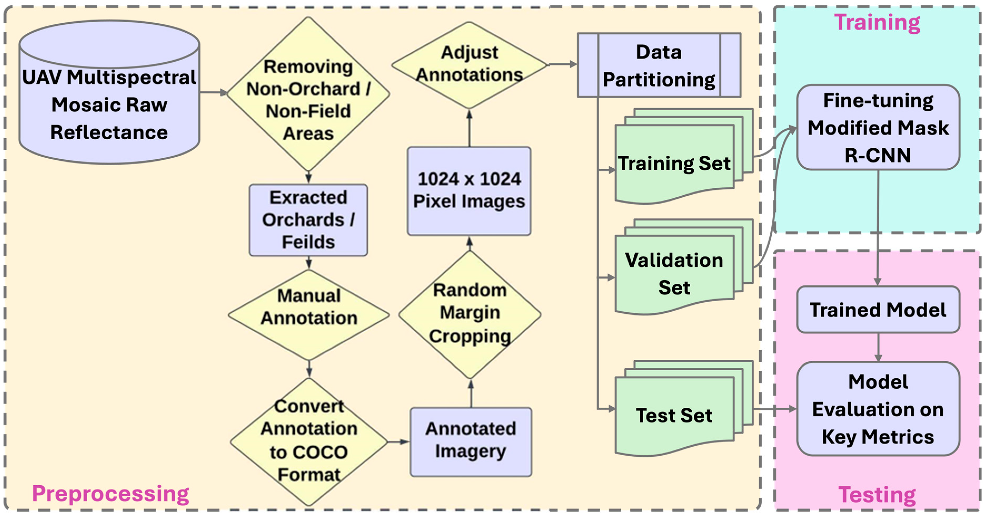
The acquired images were orthorectified and mosaicked using Pix4D photogrammetry software (Pix4D SA, Prilly, Switzerland). The resulting mosaics were processed using a methodology which has three main steps: Preprocessing, Model Training, and Evaluation (Figure 2).

2.2.1. Preprocessing

The preprocessing pipeline includes removing non-orchard areas, manual annotations of the trees with their health status, applying a random margin cropping method, and partitioning the dataset.

Removing Non-Orchard Areas

A non-orchard area removal step is introduced during preprocessing, given that the study’s objective was to assess orchard tree health on a UAV mosaic. Indeed, the UAV mosaic has portions of the landscape outside the orchards, such as roads or surrounding natural vegetation, or other crops. These irrelevant zones can dilute the model’s ability to learn features specific to apple orchards. In ArcGIS Pro, the orchard areas were manually delineated using “Polygon construction” and extracted using the “Extract by Mask” tool. Figure 3a shows the apple orchard UAV mosaic before removing non-orchard or non-field areas, and Figure 3b shows the cropped imagery showing only the four orchards.

Annotation

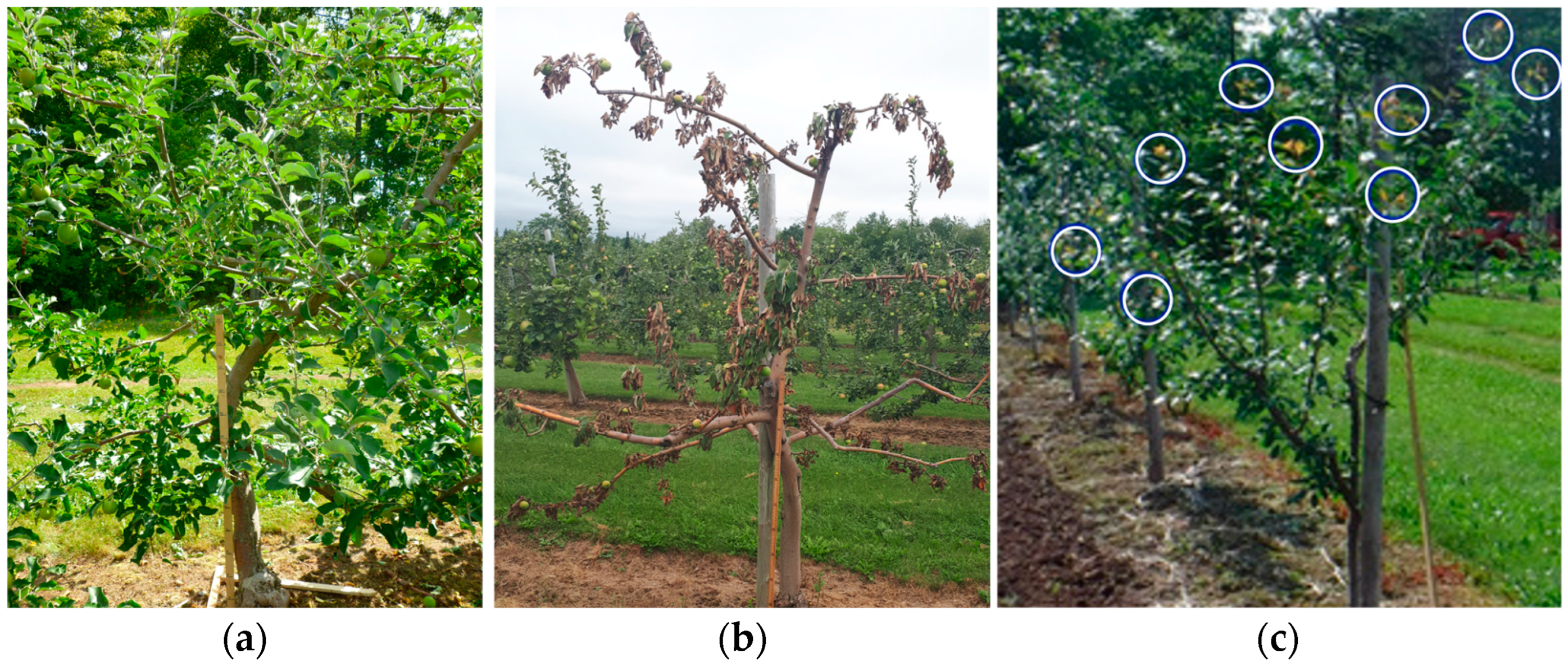
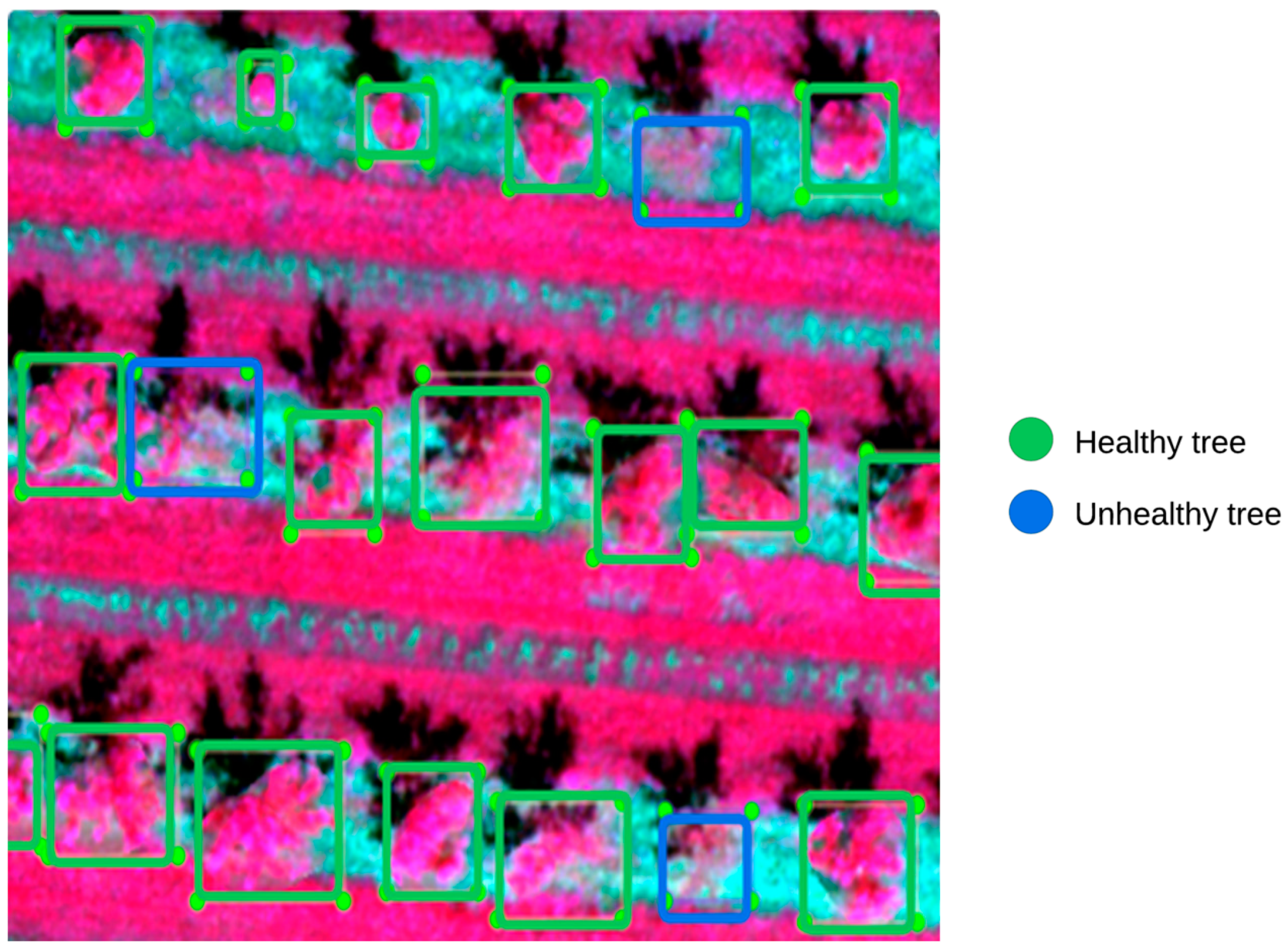
The images were manually annotated using an open-sourced software called LabelImg, which draws bounding boxes around each tree and labels each box according to the tree’s health status (healthy or unhealthy). Figure 4 shows ground pictures of a healthy and unhealthy trees, and Figure 5 shows the annotated UAV image. Manual annotation on the UAV imagery was chosen due to the lack of reliable pre-existing tree-level health labels for all trees. To improve visual separability between healthy and unhealthy trees, a NIR, Red and Green false-color composite was employed to enhance vegetation signals and facilitate more accurate photo-interpretation. Manual labeling ensures high-quality, interpretable ground truth necessary for training and evaluating the model. Automated methods such as unsupervised clustering or pretrained models were not feasible in our case, as they failed to capture subtle visual patterns related to tree health. The resulting annotations were converted into the COCO (Common Objects in Context) format to ensure compatibility with the Mask R-CNN framework.

Random Margin Cropping

Random Margin Cropping produces random margins around each bounding box on the annotated images. This process has the following objectives:

• Consistently targeted patch sizes of 1024 × 1024 pixels to be compatible with model input requirements. This ensures integration into the training without additional resizing that could cause distortion or preprocessing steps.
• Producing enough samples for a generalized model, minimizing bias during model training and validation.
• Including contextual information surrounding the trees.
• Supporting data augmentation by creating variability in the extracted patches and increasing sample diversity.

In Figure 6a, the yellow box represents a specific tree on the RGB composite. Figure 6b is a new image that results from the cropping process. All the tree annotations are then loaded on the cropped image, and their positions are adjusted to the cropped image (Figure 6c).

Data Partitioning

All the patches of 1024 × 1024 pixels were distributed among a training, validation, and test subset. The training and validation datasets were extracted from the same portion of the UAV imagery. The validation dataset was used during the training stage to monitor model performance on unseen data. The test dataset used in the study was extracted from another portion of the UAV imagery to guarantee it is truly unseen. As such, the evaluation results accurately represent the model’s ability to detect and classify objects in new and unseen environments. The UAV image covered a total orchard area of approximately 7.035 ha, which included about 4122 individual apple trees. Random margin cropping was applied to generate patches of 1024 × 1024 pixels around each tree, corresponding to a ground area of approximately 71.7 m × 71.7 m (≈0.51 ha) per patch. This process yielded a total of 4122 image patches. The cropping method itself produced augmentation, since the random margins around trees introduced variations in the extracted patches and increased dataset diversity. The dataset was divided into training, validation, and test sets following an approximate 70/15/15 split ratio. Specifically, the training and validation sets contained 2752 healthy and 785 unhealthy trees, while the test set contained 527 healthy and 58 unhealthy trees.

2.2.2. Model Training

The study used a Mask R-CNN model, which was first introduced by He et al. [48].

As shown in Figure 7, the baseline version uses, as an input image, an RGB image represented as X∈R^3×H×W, where H and W denote the image’s height and width. The model has two components: the Region of Interest (ROI) Alignment and a Detection Head.

Mask-R-CNN uses a two-stage detector, which was found to be better than one-stage alternatives, such as YOLO. As reported in Table 3, one-stage YOLOv5 models typically yield lower F1-scores (≈61.46 − 70.80%) compared to two-stage Faster R-CNN (≈93.90%) to detect trees on UAV imagery. Since our study focuses on a reliable detection of the minority class, which is made up of unhealthy trees that are both rare and difficult to detect, prioritizing accuracy over inference speed was essential. This motivated our choice of the Mask R-CNN framework despite the removal of the mask branch. Mask R-CNN has the advantage of incorporating ROI alignment (Figure 7), which improves feature alignment and benefits the detection head even when the mask branch is disabled (Figure 8, Figure 9 and Figure 10). Moreover, its modular design allowed us to incorporate multi-band (5-band) and PCA-based (3PCs) input configurations (Figure 9 and Figure 10), as well as implement class weighting and focal loss strategies during training.

A critical component of Mask R-CNN is the feature extraction backbone, which can greatly influence the model’s performance metrics. In this study, four backbones, i.e., ResNet-50, ResNet-101, ResNeXt-101, and Swin Transformer, were compared. ResNet-50 is the original backbone used in Mask R-CNN. It is a 50-layer convolutional neural network introduced by He et al. [48]. ResNet-50 has many advantages. It is known for its residual learning framework that eases the training of deep networks. It is simple, robust, fast, and has a good balance of accuracy and efficiency. Its moderate depth captures a mix of low-level and mid-level features useful for vegetation imagery (edges, textures, etc.) while keeping computational load manageable. It has approximately 26 million parameters with 3-band images [44], 41.30 million parameters with 5-band images, and requires roughly 424.85 GFLOPs for each of our 1024 × 1024 images (

Table 4. Parameters and GFLOPs of each backbone used in this study.

Backbone	Parameters (Million)		GFLOPs* Per 1024 × 1024-Pixel Image
	3-Band	5-Band
ResNet-50	26	41.30	424.85
ResNet-101	44	60.20	557.80
ResNeXt-101 (32 × 8d)	89	104.60	930.70
Swin Transformer (Base)	88	924.97	924.97

(*) GFLOPs = Giga FLOPs = billion floating-point operations (FLOPs) for a single forward pass of one image.

), making it a relatively lightweight yet powerful backbone [44]. Additionally, pretrained weights are readily available. The limitations of ResNet-50 are as follows. It may underfit small objects compared to deeper or more advanced backbones. Its downsampling stages can make very small objects harder to detect. In highly imbalanced class scenarios, ResNet-50′s feature capacity might not fully separate minority class features, potentially yielding lower recall on those minority classes.

ResNet-101 is a 101-layer version of the ResNet family, which has approximately 44 million parameters with 3-band images [44], and 60.20 million parameters with 5-band images. It has the same basic design as ResNet-50 but with additional layers. The extra layers allow it to learn more complex features, which can improve recall and precision for minority classes, which is critical for producing a high F1-score. While being more performant, ResNet-101 has an increased computation time and is more likely to overfit on limited data. ResNet-101 requires 557.80 GFLOPs per image on our test dataset (Table 4) and is slower than ResNet-50 in training the model. Its larger model size demands more GPU memory. Moreover, if the training dataset is small or poorly annotated, a deeper model might not generalize as easily as ResNet-50.

ResNeXt-101 is a complex version of ResNet [50] that introduces new parallel paths within each block called cardinalities. Unlike simply increasing depth (more layers) or width (more channels), cardinality allows the network to learn diverse, fine-grained feature representations without excessive computational cost. For this study, which has the aim of detecting small and subtle patterns such as the unhealthy trees, this diversity is crucial. Small targets occupy very few pixels in high-resolution UAV images, so subtle spectral–spatial variations may be easily lost with the standard ResNet backbones. ResNeXt’s grouped convolutions capture multiple complementary feature subspaces at different receptive fields, which enhances the model’s sensitivity to these local variations. In our study, the default ResNeXt-101 version was used, which has a 32 × 8d configuration and approximately 89 million parameters with 3-band images [42] and 104.60 million parameters with 5-band images. It can learn richer features without simply stacking more layers. The parallel convolutional channels allow capturing a variety of patterns, which is important for complex imagery like orchards, where trees may have different textures, shapes, sizes, and spectral values. Even the standard is noted to detect small objects better than ResNet 101, benefiting from multi-path feature extraction. The drawback of ResNeXt 101 is the increased complexity and resource usage. This can slow down training on large UAV datasets. Large ResNeXt models could overfit if the training data are limited or imbalanced. It needs 930.70 GFLOPs per image on our test dataset (Table 4). Overall, ResNeXt-101 is a strong candidate for high F1-score, especially when small object detection is critical and provided computational resources are available.

The Swin Transformer is a hierarchical vision transformer that replaces convolution with self-attention mechanisms applied within local image windows [46]. These windows shift across layers to allow cross-region interaction. The base Swin Transformer version has approximately 88 million parameters with 3-band images and 924.97 million parameters with 5-band images. The Swin Transformer processes features through hierarchical stages using patch partitioning and merging, functionally similar to the downsampling operations in true CNNs. This architecture allows the Swin Transformer to model long-range dependencies and multi-scale features efficiently, which is especially beneficial in complex scenes or when detecting subtle object differences. Despite its strengths, the Swin Transformer is computationally expensive, requiring 924.97 GFLOPs per image on our test dataset (Table 4). It also consumes more GPU memory and time per image compared to CNNs of similar parameter count. Swin Transformer models also tend to need larger datasets or stronger regularization, as their transformer-based architecture lacks spatial inductive biases inherent to CNNs. Without sufficient pretraining or data, performance may degrade due to overfitting. Moreover, hyperparameters such as window size and learning rate schedules are more complex to tune, and inference time may increase when applied to large UAV mosaics, even though Swin Transformer’s attention is linear in image size.

The Mask R-CNN architecture was used in three scenarios. The three scenarios differ by the input features as follows:

• Scenario 1 uses RGB images, such as in the case of the original Mask R-CNN;
• Scenario 2 is based on multispectral 5-band imagery;
• Scenario 3 involves three principal components that were computed using the multispectral 5-band reflectance images and their associated vegetation index images.

In all these scenarios, the Mask R-CNN architecture was first modified to remove the final segmentation step due to the absence of pixel-level segmentation annotations in the dataset. Indeed, given the 7 cm spatial resolution of the images, it was not feasible to determine with certainty whether a pixel belonged to a tree or not. Additionally, considering the high cost and limited benefit of producing segmentation masks under such conditions, this study focused on object detection. Although the mask branch of Mask R-CNN was removed in this work due to the lack of pixel-level annotations, the underlying framework still provides key benefits compared to directly employing Faster R-CNN.

Scenario 1: RGB Imagery

In this scenario, the original Mask R-CNN was used with the only modification of removing the segmentation step, as shown in Figure 8.

Scenario 2: Multispectral Imagery

In this scenario, the architecture was modified to handle the 5-band UAV multispectral imagery, as shown in Figure 9.

Mask R-CNN was adapted to 5-band multispectral inputs by re-parameterizing the first convolution of the backbone as follows:

• Conv1 channel expansion: The ImageNet conv1 weight tensor (64, 3, 7, 7) was replaced with (64, 5, 7, 7) so the backbone directly ingests 5 channels.
• Weight initialization: The RGB slices of conv1 were copied from the pretrained weights, and the two additional slices (Red-Edge, NIR) were initialized to zero. During fine-tuning, the network learns band-specific filters for these channels. This initialization was found stable in practice rather than adding random values to the added layers.
• Preprocessing and ordering: Bands are stacked in the order [B, G, R, RE, NIR] and standardized per band using training-set means and standard deviations.

Scenario 3: Multispectral Imagery & Vegetation Indices

In this scenario, the reflectance of all 5 multispectral bands was used along with the associated vegetation indices (VI) listed in

Table 5. Vegetation indices derived from UAV band reflectance.

Vegetation Index	Equation	Reference
Difference Vegetation Index	DVI = Near-infrared (NIR)-Red	[63]
Generalized Difference Vegetation Index	GDVI = NIR − Green	[64]
Green Normalized Difference Vegetation Index	GNDVI = (NIR − Green)/(NIR + Green)	[65]
Green-Red Vegetation Index	GRVI = NIR/Green	[64]
Normalized Difference Aquatic Vegetation Index	NDAVI = (NIR − Blue)/(NIR + Blue)	[66]
Normalized Difference Vegetation Index	NDVI = (NIR − Red)/(NIR + Red)	[63]
Normalized Difference Red-Edge	NDRE = (NIR − RedEdge)/(NIR + RedEdge)	[67]
Normalized Green	NG = Green/(NIR + Red + Green)	[62]
Normalized Red	NR = Red/(NIR + Red + Green)	[62]
Normalized NIR	NNIR = NIR/(NIR + Red + Green)	[62]
Red simple ratio Vegetation Index	RVI = NIR/Red	[68]
Water Adjusted Vegetation Index	WAVI = (1.5 × (NIR–Blue))/((NIR + Blue) + 0.5)	[66]

. These indices were selected based on their relationship with plant health [51,52,53,54]. Apple trees under stress typically show symptoms like a decrease in chlorophyll levels, red or brown spots on leaves, caused by bacterial or fungal infections [55,56], which affect the responses in specific spectral bands and thus on the related vegetation indices. The Difference Vegetation Index (DVI) and the Normalized Difference Vegetation Index (NDVI) were selected for their sensitivity to general vegetation stress indicators [57,58]. The Green NDVI (GNDVI) and the Normalized Difference Red-Edge Index (NDRE) were already shown to specifically capture chlorophyll variations [59,60,61]. The Normalized Green (NG), Normalized Red (NR), and Normalized NIR (NNIR) indices were already shown to mitigate the effects of soil background reflectance, atmospheric variation, and lighting inconsistencies [62].

Using directly the 5-band reflectance images and the associated 12 vegetation indices directly has several drawbacks: (i) it increases the dimensionality of the input, which can cause overfitting given the relatively small dataset; (ii) many indices are highly correlated (e.g., NDVI, GNDVI, RVI), leading to redundant information and additional noise; and (iii) higher input dimensionality increases the computational load. Therefore, all 17 features were transformed into three principal components in order to use only three input features. Principal Component Analysis (PCA) is a statistical technique that transforms high-dimensional data into a lower-dimensional space by selecting the principal components in the dataset. This transformation captures the maximum variance, keeping the uncorrelated features and allowing us to reduce the number of features while preserving as much of the original information as possible. PCA also helps with noise reduction by focusing on the most significant components [69].

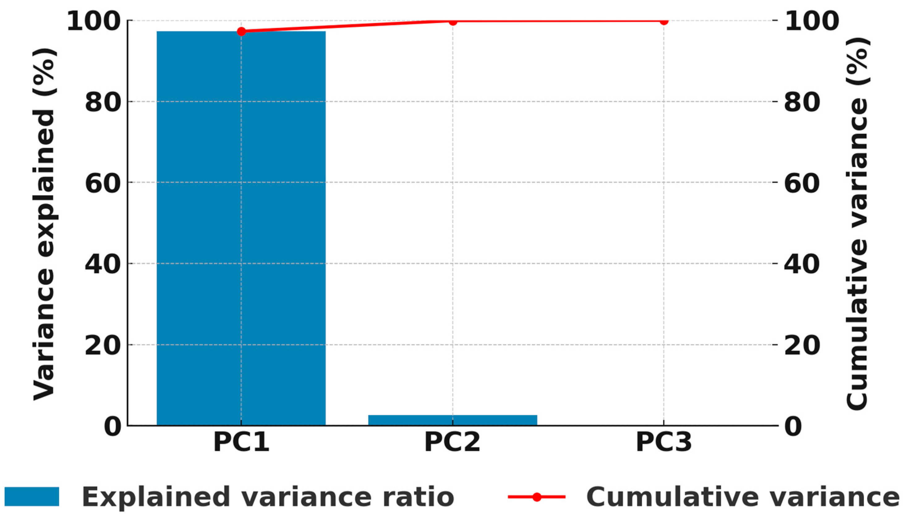
Given that vegetation indices and band reflectance can be correlated, PCA efficiently reduces their correlation and redundancy. Reducing the input channels from 17 (5 multispectral bands + 12 VIs) to 3 channels lowers the computational complexity and memory requirements for fine-tuning the Mask R-CNN model. It also lowers the computational complexity and memory requirements for fine-tuning the Mask R-CNN model, reduces the risk of overfitting, and enhances generalization to unseen images, especially when the dataset size is limited, like ours. Since PCA is sensitive to the scale of the data, PCA was applied after the standardization of the feature matrix to ensure that each feature contributes equally to the analysis. Standardization was performed by subtracting the mean and dividing by the standard deviation for each feature. The variance analysis shows that PC1 explains 97.35%, PC2 2.56%, and PC3 0.08%, leading to a cumulative variance of 99.99% (Figure 10). Therefore, nearly all discriminative information from the original 17 indices is preserved in just three components, while dimensionality reduction mitigates overfitting and reduces computation.

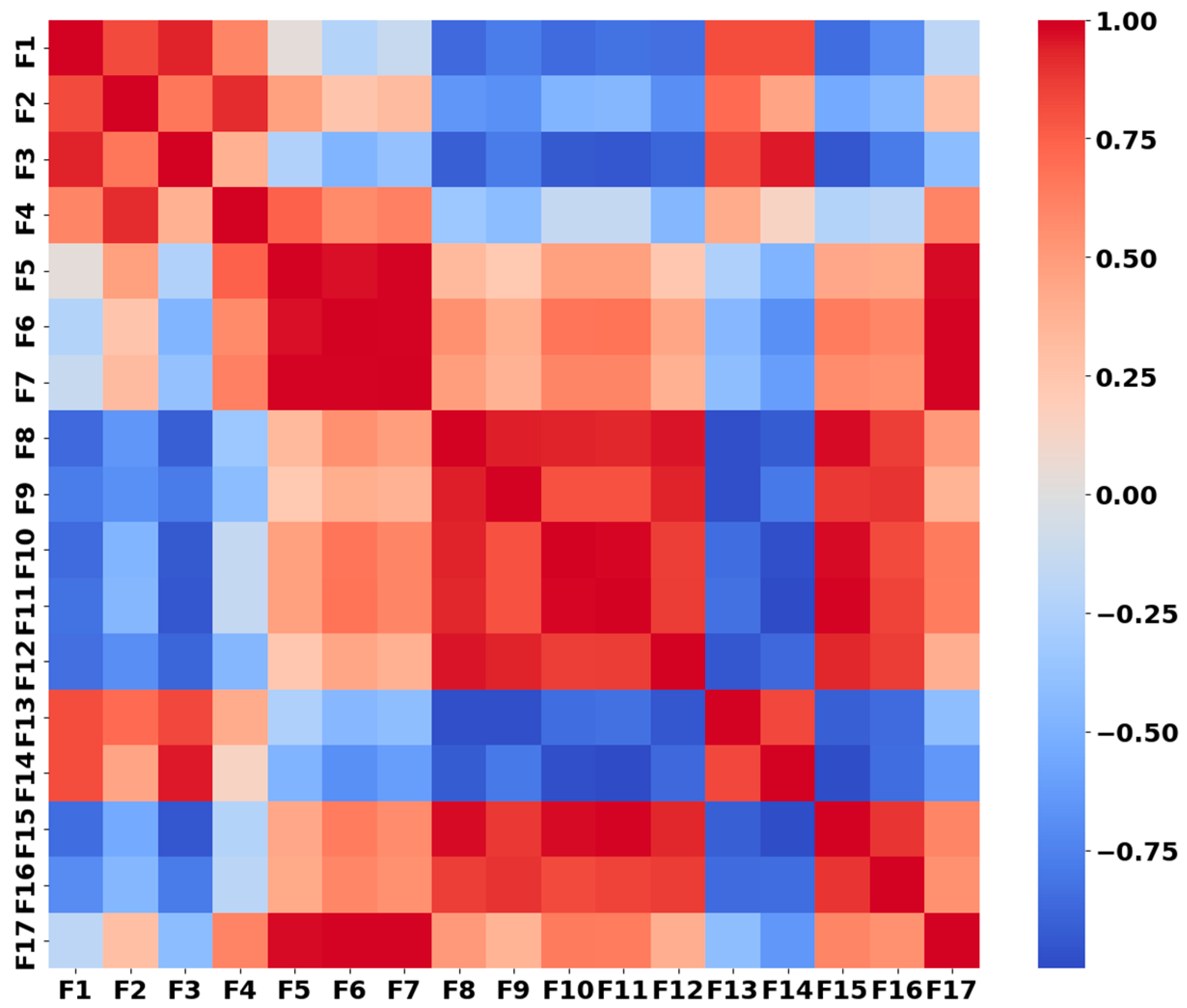
To further analyze the feature correlations, a feature correlation heatmap was generated across all 17 features. The results (Figure 11) shows that most vegetation in-dices exhibited very high correlation with each other and with the original spectral bands, particularly those involving the NIR and red reflectance, such as NDVI, GNDVI, and RVI. This indicates that the features are highly correlated and they do not provide truly independent information.

In this scenario, the Mask R-CNN architecture was modified by removing the segmentation step. The input is the top three PCs, obtained by applying PCA to 5 multispectral bands and 12 vegetation indices, as shown in Figure 12.

2.2.3. Performance Evaluation

Precision, Recall, F1-score, and mean IOU were used to evaluate the performance of the various Mask R-CNN models. To calculate these metrics, true positive (TP), false positive (FP), and false negative (FN) were calculated based on the Intersection Over Union (IoU). This variable is calculated as the overlap area between the predicted and ground truth bounding boxes divided by their union area (Equation (1)). A higher IoU indicates better localization accuracy.

$$\mathrm{IoU}={\displaystyle \frac{\mathrm{Area}\mathrm{of}\mathrm{Intersection}}{\mathrm{Area}\mathrm{of}\mathrm{Union}}}$$

(1)

An IoU threshold of 50% was used to define TP, FP, and FN. A true positive (TP) was such that the IoU between the predicted bounding box and the annotated bounding box was greater than 50% (Figure 13). Such a value indicates that the object was correctly identified and localized.

A false positive (FP) is such that the IoU was below 50% (Figure 13a). It means that the predicted bounding box did not sufficiently overlap with any ground truth boxes (Figure 13b). A false negative (FN) is such that the model does not detect or localize any ground truth boxes (Figure 13c).

Precision (Equation (2)) measures the proportion of correctly identified positive instances among all predicted positive instances.

$$\mathrm{Precision}={\displaystyle \frac{\mathrm{True}\mathrm{Positive}}{\mathrm{True}\mathrm{Positive}+\mathrm{False}\mathrm{Positive}}}$$

(2)

Recall (Equation (3)) measures the proportion of correctly identified positive instances among all positive ones.

$$\mathrm{Recall}={\displaystyle \frac{\mathrm{True}\mathrm{Positive}}{\mathrm{True}\mathrm{Positive}+\mathrm{False}\mathrm{Negative}}}$$

(3)

The F1-score (Equation (4)) represents the harmonic mean of precision and recall, providing a single metric that balances the two.

$$\mathrm{F}1\text{-}\mathrm{score}={\displaystyle \frac{2\times \mathrm{Precision}\times \mathrm{Recall}}{\mathrm{Precision}+\mathrm{Recall}}}$$

(4)

In this study, the average F1-score was calculated, which is the average of F1-scores computed across all the test samples, the Macro F1-score (Equation (5)), which is the unweighted average of the class-specific F1-scores derived from the aggregated confusion matrix, and the weighted average F1-score (Equation (6)), which is the average of class-specific F1-scores weighted by the number of samples in each class.

$$\mathrm{Macro} \text{F1-score}={\displaystyle \frac{{\mathrm{F}1\text{-}\mathrm{score}}_{healthy}+{\mathrm{F}1\text{-}\mathrm{score}}_{unhealthy}}{2}}$$

(5)

$$\mathrm{Weighted}\mathrm{Average}\mathrm{F}1\text{-}\mathrm{score}=\gamma \times {\mathrm{F}1\text{-}\mathrm{score}}_{Healthy}+\mathsf{\eta } \times {\mathrm{F}1\text{-}\mathrm{score}}_{Unhealthy},$$

(6)

where $\gamma$ and $\mathsf{\eta }$ denote the weights for healthy and unhealthy tree samples.

3. Results

Table 6. Performance metrics associated with a Mask R-CNN used to detect tree health over UAV images as a function of the image combination and the backbone. (Bold figures are the highest values in each column).

Dataset	Backbone	Average Precision (%)	Average Recall (%)	Average F1 Score (%)	Average mIoU (%)
RGB	Resnet-50	73.96	80.84	74.36	91.26
	Resnet-101	48.28	17.77	24.40	63.58
	ResneXt-101	82.39	87.65	83.46	92.18
	Swin Transformer	45.86	09.66	15.96	42.67
Multispectral	Resnet-50	80.21	79.40	77.92	91.28
	Resnet-101	73.26	45.04	53.25	84.13
	ResneXt-101	83.93	87.28	84.48	92.11
	Swin Transformer	75.23	56.59	60.42	88.02
3PCs	Resnet-50	75.67	61.97	66.77	82.20
	Resnet-101	67.91	38.50	46.95	69.93
	ResneXt-101	82.88	87.58	83.67	92.85
	Swin Transformer	14.93	44.35	17.87	72.84

shows the average precisions, recalls, F1-scores, and mIoUs for the various Mask R-CNN models applied to the three types of datasets as a function of the backbone. The highest performance across all metrics is obtained using the ResNeXt-101 backbone applied to the 5-band multispectral images. To ensure reproducibility, training was conducted with early stopping based on validation loss, and a fixed random seed was applied for weight initialization and data shuffling. Each experiment was repeated multiple times, and the reported results are averages across these runs. The repeated experiments yielded very similar outcomes, demonstrating the stability and robustness of the model performance.

The dataset is highly unbalanced. In the training and validation sets, there are 2752 healthy and 785 unhealthy trees, while the test set contains 527 healthy and 58 unhealthy trees. To address class imbalance during training, a class weighting scheme was applied based on the inverse frequency of each class. The weight w for class c is computed by (Equation (7)).

$$w={\displaystyle \frac{\mathrm{N}}{\mathrm{c}}},$$

(7)

where N is the total number of samples across all classes, and c’ is the number of samples in class c.

Equation (7) ensures that classes with fewer instances are assigned higher weights, encouraging the model to consider underrepresented classes better.

Table 7. Performance metrics associated with a Mask R-CNN used to detect tree health over UAV images as a function of the image combination and the backbone after incorporating class weighting into the algorithm. (Bold figures are the highest values in each column).

Dataset	Backbone	Average Precision (%)	Average Recall (%)	Average F1-Score (%)	Average mIoU (%)
RGB	Resnet-50	78.54	85.65	80.53	90.68
	Resnet-101	48.06	17.63	24.83	76.05
	ResneXt-101	82.71	87.00	83.64	92.23
	Swin Transformer	48.53	13.45	21.06	47.12
Multispectral	Resnet-50	79.84	79.78	77.92	91.07
	Resnet-101	68.22	34.83	43.37	82.02
	ResneXt-101	85.15	88.18	85.70	92.85
	Swin Transformer	75.55	62.06	63.94	86.21
3PCs	Resnet-50	75.98	73.01	73.78	88.86
	Resnet-101	73.63	58.69	64.42	87.55
	ResneXt-101	82.46	86.22	82.75	92.93
	Swin Transformer	54.52	22.91	31.25	84.10

lists the performance metrics associated with each Mask R-CNN applied to UAV images as a function of the image combination and the backbone, after applying class weights. Adding class weights during training moderately improved performance. The highest performance across all metrics is again obtained using the ResNeXt-101 backbone with 5-band multispectral images.

To further address the class imbalance, the standard cross-entropy loss function was replaced with the focal loss function. Unlike the standard cross-entropy loss function, the focal loss function reduces the contribution of easy, well-classified cases and concentrates learning on hard-to-classify cases. This is particularly advantageous in object detection tasks involving minority classes, where predictions tend to be biased toward dominant classes.

Table 8. A comparison between the loss function for the confusion matrix is computed when the ResNeXt-101 Mask R-CNN with class weight is applied to the 5-band multispectral images. (Bold figures are the highest values in each column).

Loss Function	Prediction	Ground Truth
		Healthy Trees	Unhealthy Trees	Accuracy (%)
Cross Entropy	Healthy trees	467	5	95.99
	Unhealthy trees	15	12
Focal	Healthy trees	452	13	95.58
	Unhealthy trees	9	24

presents the confusion matrices comparing predictions under the two loss function configurations. With the standard cross-entropy loss function, the model achieved high class precision for the healthy tree class but not for the unhealthy tree class. When using the focal loss function, the recall for the minority class (unhealthy trees) is improved as the true positive detection of unhealthy trees increased from 12 to 24.

Table 9. Model performance metrics as a function of the loss function when a Mask R-CNN with a ResneXt-101 backbone is applied to the 5-band multispectral UAV images. (Bold figures are the highest values in each column).

Loss Function	Average Precision (%)		mAP@50 (%)	Average F1-Score (%)	Macro F1-Score (%)	Weighted Average F1-Score
	Healthy Trees	Unhealthy Trees
Cross Entropy	90.18	39.32	64.75	85.70	76.22	93.60
Focal	90.73	42.76	66.74	84.18	83.10	94.76

presents the performance metrics of the Mask R-CNN model with a ResNeXt-101 backbone applied to 5-band multispectral imagery as a function of the loss function. While the model exhibits high performance for the majority class (healthy trees), detection of the minority class (unhealthy trees) remains challenging due to class imbalance. The use of the focal loss function improves the average precision (AP) for the unhealthy tree class by 3.44%, the macro-F1-score by 6.88% and the weighted average F1-score by 1.16%, which shows a higher sensitivity to the minority class without significantly compromising overall performance.

Figure 14 visually compares the trees that the model detected to the annotated ones. The annotated trees are represented in white in the case of healthy trees and red in the case of unhealthy trees. The model-detected trees are represented in blue in the case of healthy trees and yellow in the case of unhealthy trees. The model effectively identifies most healthy trees, but is less effective at detecting the unhealthy trees. Although detecting unhealthy trees improved after applying class weighting and focal loss, some missed or misclassified trees remain, especially where there are overlapped canopies or where the spectral differences are too subtle. Figure 14a shows very distinguished trees that were detected more accurately and Figure 14b shows crowded tree crowns that are more challenging for the model to detect them.

As shown in Figure 14, most FP cases in our study are not related to detecting non-tree regions (e.g., soil or background), but rather are due to class confusions between healthy and unhealthy trees. As a result, an unhealthy tree (ground truth: red box) may be misclassified as healthy (prediction: blue box). The predicted healthy tree therefore counts as an FP, and the missed unhealthy tree simultaneously counts as an FN.

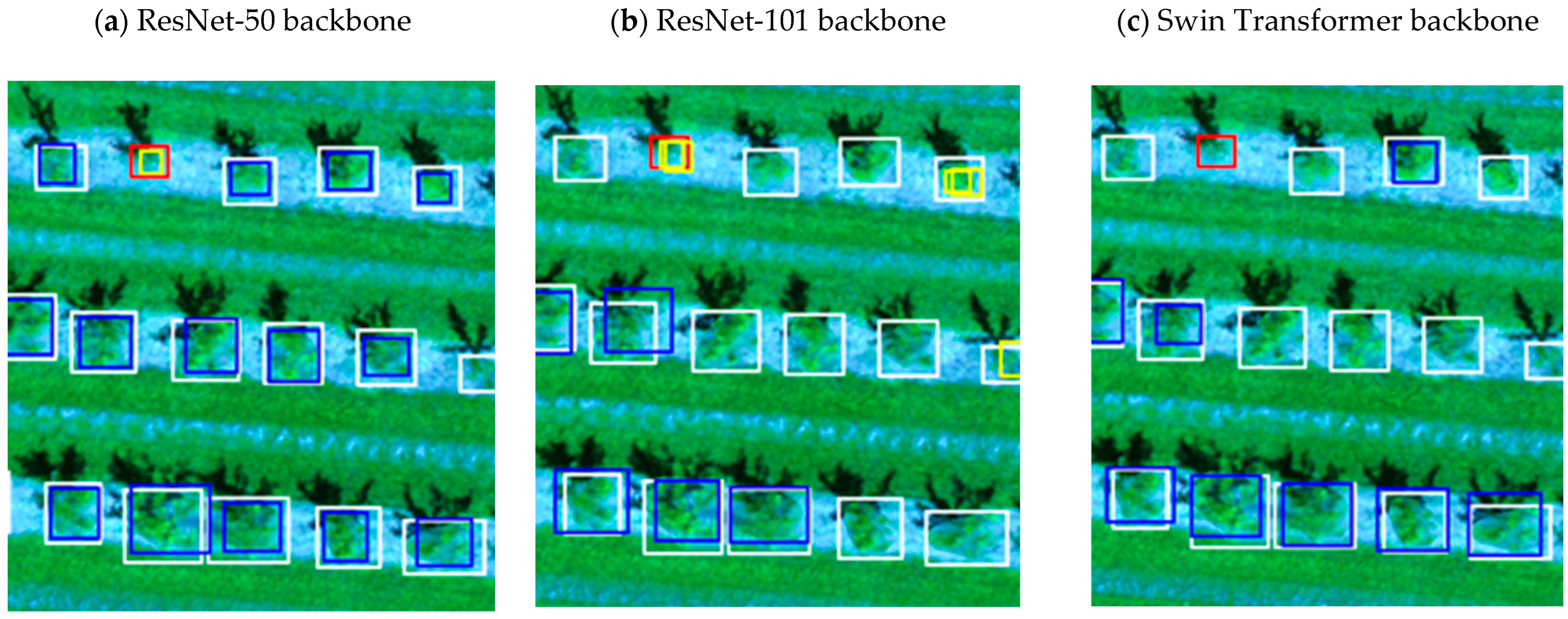
Figure 15 visually compares the outputs from the Mask R-CNN model with ResNet-50, ResNet-101, and Swin Transformer backbones.

4. Discussion

Mask R-CNN has consistently shown superior F1-score in tree detection tasks [4,5,6,7,8] compared to YOLO-based models [3,29,30]. Kaviani et al. (2023) [30] evaluated YOLOv7 and YOLOv8 for tree detection on the same dataset. The results showed that YOLOv7 underperformed compared to our current approach, and YOLOv8 did not improve over YOLOv7. Its performance was lower. Therefore, the present study used a Mask R-CNN–based framework, which simultaneously detects tree crowns and classifies their health status.

Mask R-CNN was applied with four different backbones (Resnet-50, Resnet-101, ResneXt-101, and Swin Transformer) to three image combinations (RGB, 5-band multispectral images, and 3PCs) in two different conditions (unweighted classes and weighted classes). The best F1-score (94.76%) was achieved when a Mask R-CNN having a ResNeXt-101 backbone, weighted classes, and a focal loss function, was applied to the 5-band multispectral imagery. The imbalanced data were further addressed by changing the cross-entropy loss function to the focal loss function. This makes the F1-score slightly lower (by 1.52%) because the model focuses more on the minority class (unhealthy trees) and is less sensitive to the majority class (healthy trees). Better detection of the minority class is more important in our case because the goal of our study was to detect unhealthy trees. Our F1-score is higher than those of previous studies that applied YOLOv5 [17,18,19] (61.46%) and Faster R-CNN (93.90%; [16]). Win et al. (2023) [15] achieved a better F1-score (98.55%) than what this study did, but they used UAV images acquired over oil palm trees, which have larger crowns and are easier to detect.

The best model has ResNeXt-101 as a backbone. Mask R-CNN with a ResNet-101 backbone produced better results than ResNet-50 backbone because of the deeper layers. Compared to ResNet-101, which has similar depths, ResNeXt-101 consistently achieved higher F1-scores (Table 6 and Table 7), confirming that the depth of the CNN is not enough to explain the model performance.

The highest performance of the ResNeXt-101 backbone is because it uses cardinality (multiple paths within each residual block) to increase representational power. Such an architectural design allows the model to capture finer-grained features, which is especially critical in identifying trees that can be too small (like very young or dead trees) and subtle signs of unhealthy trees on UAV imagery. While achieving higher F1-scores, ResNeXt-101 requires more than twice the computational load of ResNet-50 (930.70 GFLOPs versus 424.85 GFLOPs for each 1024 × 1024 image) (Table 4). Swin Transformer backbones theoretically offer better spatial relationships via self-attention than ResNet backbones, but in our case, the Swin Transformer backbone gave a limited performance due to overfitting related to our small dataset size, which prevents having a good training of the model. The dataset size is less important for ResNeXt backbones, which benefit more from transfer learning with limited data. To further examine the Swin Transformer’s potential, progressive layer-wise fine-tuning combined with class weighting was applied during the ImageNet fine-tuning stage. However, the evaluation on multispectral UAV imagery showed that these strategies did not stabilize the model’s performance. Specifically, the Swin Transformer achieved an Average Precision (AP) of 69.83%, Average Recall of 27.21%, Average F1 Score of 32.70%, and an Average mIoU of 67.79%. Class-specific analysis revealed that the AP for healthy trees was 35.32%, while the AP for unhealthy trees dropped to only 4.45%, resulting in a mAP@50 of 19.89%. Moreover, the Swin Transformer continued to underperform relative to ResNeXt-101, particularly for the minority unhealthy-tree class, where recall and AP remained low. Probably, the Swin Transformer requires either substantially larger and more diverse datasets or stronger regularization strategies to fully leverage its theoretical advantages.

Our dataset has highly imbalanced classes (2752 healthy trees vs. 785 unhealthy trees in the validation and training sets, and 527 healthy trees vs. 58 unhealthy trees in the test set). This imbalance was addressed by (1) computing class weights based on inverse frequency and (2) replacing the standard cross-entropy loss function (which caused the model to overfit to the dominant class (healthy trees) with a focal loss function to emphasize the minority class. The focal loss function down-weights well-classified examples and concentrates the training on harder, misclassified samples. This proved especially beneficial in our case, where unhealthy trees were rare and diverse in appearance. As shown in Table 9, despite a minor trade-off in precision for the majority class, the overall detection performance improved significantly. The focal loss function increased recall for the unhealthy tree class from 27.27% to 60.00%. This led to a 3.44% average precision improvement for the unhealthy tree class (from 39.32% to 42.76%) and a mAP gain of 2%, showing that our weighting strategy successfully improved the model’s sensitivity toward the minority class. The undersampling method was not employed as this would have further reduced the already limited number of healthy samples, leading to the loss of valuable information. The oversampling strategy (SMOTE) was tested, but it did not improve the results. In fact, while the overall precision and recall remained high (Average Precision = 84.63%, Average Recall = 87.63%, Average F1-score = 84.63%, Average mIoU = 91.34%, AP for healthy trees = 93.10%), the AP for unhealthy trees remained as low as 36.90%, which is less than the reported results. This is attributed to the limited diversity of unhealthy tree samples in the dataset. Therefore, oversampling leads to repeated exposure of the same few patterns, which increases the risk of overfitting but does not add new discriminative information.

For all the backbones, the F1-scores were higher with the 5-band multispectral images than with the RGB images. This was expected as the 5-band Images include the Red-Edge and Near-Infrared band reflectance, both being sensitive to leaf chlorophyll content that is a good indicator of tree health [51,56]. This study also tested a third image combination that consisted of three principal components computed from the 5-band reflectance and the 12 vegetation index images through a PCA This method decreases computational cost and overfitting risk by reducing 17 channels into three principal components. The corresponding F1-score (82.75%) was below the one computed with the 5-band reflectance image combination (85.70%). The lack of performance associated with adding vegetation indices is probably related to the redundancy of information between the vegetation index images and the 5-band reflectance images.

In our experiments, the model with the ResNet-101 backbone was less performant than the model with the ResNet-50 backbone. This shows that simply stacking more layers in the ResNet family does not bring better performances. Consequently, extending further to ResNet-152 would likely add computational cost without a real benefit. Given that the model with a ResNet-50 backbone performed worse than the model with a ResNeXt-101 backbone, we can expect that using a model with a ResNet-34 backbone will be less performant than the model with a ResNeXt-101 backbone.

The study by Jiang et al. [16] (Table 3) reporting a 93.9% F1-score with Faster R-CNN applied to RGB images was conducted on broadleaved trees and conifers, focusing exclusively on detecting dead trees that do not have leaves rather than detecting trees according to their health status. This is different from our work, which addresses a more challenging task of distinguishing healthy vs. unhealthy apple trees on multispectral UAV imagery. Indeed, instead of detecting only dead trees, our study involves fine-grained detection of healthy and unhealthy trees that have subtle spectral differences. In addition, the crowns of apple trees are smaller and less distinct than those of mature broad-leaved and coniferous trees. Another difference with our study is that Jiang et al. [16] used images with a pixel size of 5.1cm, while in our case, we used images having a pixel size of 7cm. Therefore, while a high F1-score highlights the potential of Faster R-CNN on large-crown forest trees with binary labels, the study by Jiang et al. [16] cannot be directly compared with our results.

The dataset used in this study is limited to a single orchard in 2018. We fully acknowledge that this represents a limitation on our work. The restricted dataset constrains the generalization ability of the model across different orchards, seasons, and tree species. However, this work was designed as a pilot study, aiming to test the feasibility of combining UAV multispectral imagery with deep learning for orchard tree health detection. In future work, we plan to extend the dataset to include multiple orchards, seasons, and tree species in order to further validate the generalizability of the model.

Although our current study does not include direct economic or yield data from orchards, the existing literature has already reported the significant economic impact of plant diseases and the potential benefits of early detection. According to the Food and Agriculture Organization (FAO), 20–40% of global crop production is lost annually due to plant pests and diseases [70]. In a study where hyperspectral images were tested, Shadrin et al. [71] show that apple scab can result in yield losses of 50–60%.

5. Conclusions

This study applied a single-step method using a Mask R-CNN model to 5-band UAV multispectral imagery to detect the health status of orchard apple trees. Three different input data configurations (RGB, 5-band multispectral images, and 3PCs) and four backbone architectures (Resnet-50, Resnet-101, ResNeXt-101, and Swin Transformer) was considered in this study. The highest average F1-score (85.68%) and mean IoU (92.85%) were obtained with the ResNeXt-101 backbone applied to the 5-band multispectral imagery. The Swin Transformer underperformed in our study due to overfitting on the limited dataset and its reliance on large-scale data for effective training [46], unlike ResNeXt-101, which benefits from transfer learning with smaller datasets due to its robust feature extraction capabilities [50].

Our dataset was imbalanced between the healthy and unhealthy tree classes, given a significantly higher number of healthy trees in the orchard. The class imbalance was addressed by applying class weighting and replacing the standard loss function with the focal loss function during training. These changes improved the detection of unhealthy trees and helped the model become more sensitive to the minority class. The 5-band multispectral image clearly outperformed the RGB image combination, showing the importance of including Red-Edge and NIR bands for monitoring vegetation health. Using additional information from the vegetation index images did not improve the F1-score.

Our study was based on a single-species case with a limited tree dataset. Future work should incorporate larger and more diverse tree datasets from different orchards and seasons, which could improve the generalization of results. The study only considered orchard trees, and it would be appropriate to test the method on other case studies in agriculture and forestry. The study only detected healthy and unhealthy trees, and future work is needed to develop a method for detecting the tree health status and the causes that produce unhealthy trees. Despite these limitations, the proposed one-step methodology offers a scalable and accurate solution for orchard tree health monitoring using 5-band multispectral UAV images. The methodology workflow was simplified by combining the tree detection and health classification into a single step, making it easier to apply in real-world scenarios.

References

1. Eugenio, F.C.; Schons, C.T.; Mallmann, C.L.; Schuh, M.S.; Fernandes, P.; Badin, T.L. Remotely piloted aircraft systems and forests: A global state of the art and future challenges. Can. J. For. Res. 2020, 50, 705–716. [Google Scholar] [CrossRef]
2. Ecke, S.; Dempewolf, J.; Frey, J.; Schwaller, A.; Endres, E.; Klemmt, H.J.; Tiede, D.; Seifert, T. UAV-based forest health monitoring: A systematic review. Remote Sens. 2022, 14, 3205. [Google Scholar] [CrossRef]
3. Jemaa, H.; Bouachir, W.; Leblon, B.; LaRocque, A.; Haddadi, A.; Bouguila, N. UAV-based computer vision system for orchard apple tree detection and health assessment. Remote Sens. 2023, 15, 3558. [Google Scholar] [CrossRef]
4. Li, H.; Chen, L.; Yao, Z.; Li, N.; Long, L.; Zhang, X. Intelligent identification of pine wilt disease infected individual trees using UAV-based hyperspectral imagery. Remote Sens. 2023, 15, 3295. [Google Scholar] [CrossRef]
5. Miraki, M.; Sohrabi, H.; Fatehi, P.; Kneubuehler, M. Detection of mistletoe infected trees using UAV high spatial resolution images. J. Plant Dis. Prot. 2021, 128, 1679–1689. [Google Scholar] [CrossRef]
6. Guerra-Hernández, J.; Díaz-Varela, R.A.; Ávarez-González, J.G.; Rodríguez-González, P.M. Assessing a novel modelling approach with high resolution UAV imagery for monitoring health status in priority riparian forests. For. Ecosyst. 2021, 8, 61. [Google Scholar] [CrossRef]
7. Naseri, M.H.; Shataee Jouibary, S.; Habashi, H. Analysis of forest tree dieback using UltraCam and UAV imagery. Scand. J. For. Res. 2023, 38, 392–400. [Google Scholar] [CrossRef]
8. Brovkina, O.; Cienciala, E.; Surový, P.; Janata, P. Unmanned Aerial Vehicles (UAV) for assessment of qualitative classification of Norway spruce in temperate forest stands. Geo-Spat. Inf. Sci. 2018, 21, 12–20. [Google Scholar] [CrossRef]
9. Moriya, É.A.; Imai, N.N.; Tommaselli, A.M.; Berveglieri, A.; Santos, G.H.; Soares, M.A.; Marino, M.; Reis, T.T. Detection and mapping of trees infected with citrus gummosis using UAV hyperspectral data. Comput. Electron. Agric. 2021, 188, 106298. [Google Scholar] [CrossRef]
10. Näsi, R.; Honkavaara, E.; Lyytikäinen-Saarenmaa, P.; Blomqvist, M.; Litkey, P.; Hakala, T.; Viljanen, N.; Kantola, T.; Tanhuanpää, T.; Holopainen, M. Using UAV-based photogrammetry and hyperspectral imaging for mapping bark beetle damage at tree-level. Remote Sens. 2015, 7, 15467–15493. [Google Scholar] [CrossRef]
11. Näsi, R.; Honkavaara, E.; Blomqvist, M.; Lyytikäinen-Saarenmaa, P.; Hakala, T.; Viljanen, N.; Kantola, T.; Holopainen, M. Remote sensing of bark beetle damage in urban forests at individual tree level using a novel hyperspectral camera from UAV and aircraft. Urban For. Urban Green. 2018, 30, 72–83. [Google Scholar] [CrossRef]
12. Zhang, N.; Wang, Y.; Zhang, X. Extraction of tree crowns damaged by Dendrolimus tabulaeformis Tsai et Liu via spectral-spatial classification using UAV-based hyperspectral images. Plant Methods 2020, 16, 135. [Google Scholar] [CrossRef]
13. Honkavaara, E.; Näsi, R.; Oliveira, R.; Viljanen, N.; Suomalainen, J.; Khoramshahi, E.; Hakala, T.; Nevalainen, O.; Markelin, L.; Vuorinen, M.; et al. Using multitemporal hyper-and multispectral UAV imaging for detecting bark beetle infestation on Norway spruce. Int. Arch. Photogramm. Remote Sens. Spat. Inf. Sci. 2020, 43, 429–434. [Google Scholar] [CrossRef]
14. Barmpoutis, P.; Stathaki, T.; Kamperidou, V. Monitoring of trees’ health condition using a UAV equipped with low-cost digital camera. In Proceedings of the IEEE International Conference on Acoustics, Speech and Signal Processing (ICASSP 2019), Brighton, UK, 12–17 May 2019. [Google Scholar]
15. Kent, O.W.; Chun, T.W.; Choo, T.L.; Kin, L.W. Early symptom detection of basal stem rot disease in oil palm trees using a deep learning approach on UAV images. Comput. Electron. Agric. 2023, 213, 108192. [Google Scholar] [CrossRef]
16. Jiang, X.; Wu, Z.; Han, S.; Yan, H.; Zhou, B.; Li, J. A multi-scale approach to detecting standing dead trees in UAV RGB images based on improved faster R-CNN. PLoS ONE. 2023, 18, e0281084. [Google Scholar] [CrossRef]
17. Dolgaia, L.; Illarionova, S.; Nesteruk, S.; Krivolapov, I.; Baldycheva, A.; Somov, A.; Shadrin, D. Apple tree health recognition through the application of transfer learning for UAV imagery. In Proceedings of the IEEE 28th International Conference on Emerging Technologies and Factory Automation (ETFA 2023), Sinaia, Romania, 12–15 September 2023. [Google Scholar]
18. Hofinger, P.; Klemmt, H.J.; Ecke, S.; Rogg, S.; Dempewolf, J. Application of YOLOv5 for point label based object detection of black pine trees with vitality losses in UAV data. Remote Sens. 2023, 15, 1964. [Google Scholar] [CrossRef]
19. Puliti, S.; Astrup, R. Automatic detection of snow breakage at single tree level using YOLOv5 applied to UAV imagery. Int. J. Appl. Earth Obs. Geoinf. 2022, 112, 102946. [Google Scholar] [CrossRef]
20. Wang, Y.; Zhu, X.; Wu, B. Automatic detection of individual oil palm trees from UAV images using HOG features and an SVM classifier. Int. J. Remote Sens. 2019, 40, 7356–7370. [Google Scholar] [CrossRef]
21. Erdem, F.; Ocer, N.E.; Matci, D.K.; Kaplan, G.; Avdan, U. Apricot tree detection from UAV-images using mask R-CNN and U-NET. Photogramm. Eng. Remote Sens. 2023, 89, 89–96. [Google Scholar] [CrossRef]
22. Șandric, I.; Irimia, R.; Petropoulos, G.P.; Anand, A.; Srivastava, P.K.; Pleșoianu, A.; Faraslis, I.; Stateras, D.; Kalivas, D. Tree’s detection & health’s assessment from ultra-high resolution UAV imagery and deep learning. Geocarto Int. 2022, 37, 10459–10479. [Google Scholar]
23. Gibril, M.B.; Shafri, H.Z.; Shanableh, A.; Al-Ruzouq, R.; Wayayok, A.; Hashim, S.J.; Sachit, M.S. Deep convolutional neural networks and Swin transformer-based frameworks for individual date palm tree detection and mapping from large-scale UAV images. Geocarto Int. 2022, 37, 18569–18599. [Google Scholar] [CrossRef]
24. Yu, K.; Hao, Z.; Post, C.J.; Mikhailova, E.A.; Lin, L.; Zhao, G.; Tian, S.; Liu, J. Comparison of classical methods and mask R-CNN for automatic tree detection and mapping using UAV imagery. Remote Sens. 2022, 14, 295. [Google Scholar] [CrossRef]
25. Safonova, A.; Guirado, E.; Maglinets, Y.; Alcaraz-Segura, D.; Tabik, S. Olive tree biovolume from UAV multi-resolution image segmentation with Mask R-CNN. Sensors 2021, 21, 1617. [Google Scholar] [CrossRef]
26. Lobo Torres, D.; Queiroz Feitosa, R.; Nigri Happ, P.; Elena Cué La Rosa, L.; Marcato Junior, J.; Martins, J.; Olã Bressan, P.; Gonçalves, W.N.; Liesenberg, V. Applying fully convolutional architectures for semantic segmentation of a single tree species in urban environment on high resolution UAV optical imagery. Sensors 2020, 20, 563. [Google Scholar] [CrossRef]
27. Ferreira, M.P.; de Almeida, D.R.; de Almeida Papa, D.; Minervino, J.B.; Veras, H.F.; Formighieri, A.; Santos, C.A.; Ferreira, M.A.; Figueiredo, E.O.; Ferreira, E.J. Individual tree detection and species classification of Amazonian palms using UAV images and deep learning. For. Ecol. Manag. 2020, 475, 118397. [Google Scholar] [CrossRef]
28. Kestur, R.; Angural, A.; Bashir, B.; Omkar, S.N.; Anand, G.; Meenavathi, M.B. Tree crown detection, delineation and counting in UAV remote sensed images: A neural network based spectral–spatial method. J. Indian Soc. Remote Sens. 2018, 46, 991–1004. [Google Scholar] [CrossRef]
29. Wang, J.; Zhang, H.; Liu, Y.; Zhang, H.; Zheng, D. Tree-Level Chinese Fir Detection Using UAV RGB Imagery and YOLO-DCAM. Remote Sens. 2024, 16, 335. [Google Scholar] [CrossRef]
30. Kaviani, M.; Akilan, T.; Leblon, B.; Amishev, D.; Haddadi, A.; LaRocque, A. Comparison of YOLOv7 and YOLOv8n for tree detection on UAV RGB imagery. In Proceedings of the 45th Canadian Symposium on Remote Sensing, Halifax, NS, Canada, 10–13 June 2024. [Google Scholar]
31. Moradi, F.; Javan, F.D.; Samadzadegan, F. Potential evaluation of visible-thermal UAV image fusion for individual tree detection based on convolutional neural network. Int. J. Appl. Earth Obs. Geoinf. 2022, 113, 103011. [Google Scholar] [CrossRef]
32. Ghasemi, M.; Latifi, H.; Pourhashemi, M. A novel method for detecting and delineating coppice trees in UAV images to monitor tree decline. Remote Sens. 2022, 14, 5910. [Google Scholar] [CrossRef]
33. Al Mansoori, S.; Kunhu, A.; Al Ahmad, H. Automatic palm trees detection from multispectral UAV data using normalized difference vegetation index and circular Hough transform. In Proceedings of the SPIE Remote Sensing, Berlin, Germany, 10–13 September 2018. [Google Scholar]
34. Ampatzidis, Y.; Partel, V. UAV-based high throughput phenotyping in citrus utilizing multispectral imaging and artificial intelligence. Remote Sens. 2019, 11, 410. [Google Scholar] [CrossRef]
35. Suab, S.A.; Syukur, M.S.; Avtar, R.; Korom, A. Unmanned Aerial Vehicle (UAV) derived normalised difference vegetation index (NDVI) and crown projection area (CPA) to detect health conditions of young oil palm trees for precision agriculture. Int. Arch. Photogramm. Remote Sens. Spat. Inf. Sci. 2019, 42, 611–614. [Google Scholar] [CrossRef]
36. Anisa, M.N.; Hernina, R. UAV application to estimate oil palm trees health using Visible Atmospherically Resistant Index (VARI) (Case study of Cikabayan Research Farm, Bogor City). In Proceedings of the 2nd International Conference on Sustainable Agriculture and Food Security (ICSAFS), West Java, Indonesia, 28–29 October 2020. [Google Scholar]
37. Marques, P.; Pádua, L.; Adão, T.; Hruška, J.; Peres, E.; Sousa, A.; Sousa, J.J. UAV-based automatic detection and monitoring of chestnut trees. Remote Sens. 2019, 11, 855. [Google Scholar] [CrossRef]
38. Wu, Y.; Li, X.; Zhang, Q.; Zhou, X.; Qiu, H.; Wang, P. Recognition of spider mite infestations in jujube trees based on spectral-spatial clustering of hyperspectral images from UAVs. Front. Plant Sci. 2023, 14, 1078676. [Google Scholar] [CrossRef]
39. Safonova, A.; Tabik, S.; Alcaraz-Segura, D.; Rubtsov, A.; Maglinets, Y.; Herrera, F. Detection of fir trees (Abies sibirica) damaged by the bark beetle in unmanned aerial vehicle images with deep learning. Remote Sens. 2019, 11, 643. [Google Scholar] [CrossRef]
40. Bergmüller, K.O.; Vanderwel, M.C. Predicting tree mortality using spectral indices derived from multispectral UAV imagery. Remote Sens. 2022, 14, 2195. [Google Scholar] [CrossRef]
41. Hu, G.; Yin, C.; Wan, M.; Zhang, Y.; Fang, Y. Recognition of diseased Pinus trees in UAV images using deep learning and AdaBoost classifier. Biosyst. Eng. 2020, 194, 138–151. [Google Scholar] [CrossRef]
42. Iqbal, M.S.; Ali, H.; Tran, S.N.; Iqbal, T. Coconut trees detection and segmentation in aerial imagery using mask region-based convolution neural network. IET Comput. Vis. 2021, 15, 428–439. [Google Scholar] [CrossRef]
43. Mo, J.; Lan, Y.; Yang, D.; Wen, F.; Qiu, H.; Chen, X.; Deng, X. Deep learning-based instance segmentation method of litchi canopy from UAV-acquired images. Remote Sens. 2021, 13, 3919. [Google Scholar] [CrossRef]
44. Elharrouss, O.; Akbari, Y.; Almadeed, N.; Al-Maadeed, S. Backbones-review: Feature extractor networks for deep learning and deep reinforcement learning approaches in computer vision. Comput. Sci. Rev. 2024, 53, 100645. [Google Scholar] [CrossRef]
45. Li, Y.; Wang, H.; Dang, L.M.; Song, H.K.; Moon, H. Orcnn-x: Attention-driven multiscale network for detecting small objects in complex aerial scenes. Remote Sens. 2023, 15, 3497. [Google Scholar] [CrossRef]
46. Liu, Z.; Lin, Y.; Cao, Y.; Hu, H.; Wei, Y.; Zhang, Z.; Lin, S.; Guo, B. Swin transformer: Hierarchical vision transformer using shifted windows. In Proceedings of the IEEE/CVF International Conference on Computer Vision Workshops (ICCVW), Montreal, QC, Canada, 11–17 October 2021. [Google Scholar]
47. Jeevan, P.; Sethi, A. Which backbone to use: A resource-efficient domain specific comparison for computer vision. arXiv 2024, arXiv:2406.05612. [Google Scholar] [CrossRef]
48. He, K.; Gkioxari, G.; Dollár, P.; Girshick, R. Mask R-CNN. In Proceedings of the IEEE International Conference on Computer Vision (ICCV), Venice, Italy, 22–29 October 2017. [Google Scholar]
49. Arjoune, Y.; Peri, S.; Sugunaraj, N.; Biswas, A.; Sadhukhan, D.; Ranganathan, P. An instance segmentation and clustering model for energy audit assessments in built environments: A multi-stage approach. Sensors 2021, 21, 4375. [Google Scholar] [CrossRef]
50. Xie, S.; Girshick, R.; Dollár, P.; Tu, Z.; He, K. Aggregated residual transformations for deep neural networks. In Proceedings of the IEEE Conference on Computer Vision and Pattern Recognition (CVPR), Honolulu, HI, USA, 21–26 July 2017. [Google Scholar]
51. Dash, J.P.; Watt, M.S.; Pearse, G.D.; Heaphy, M.; Dungey, H.S. Assessing very high resolution UAV imagery for monitoring forest health during a simulated disease outbreak. ISPRS J. Photogramm. Remote Sens. 2017, 131, 1–14. [Google Scholar] [CrossRef]
52. Cogato, A.; Pagay, V.; Marinello, F.; Meggio, F.; Grace, P.; De Antoni Migliorati, M. Assessing the feasibility of using Sentinel-2 imagery to quantify the impact of heatwaves on irrigated vineyards. Remote Sens. 2019, 11, 2869. [Google Scholar] [CrossRef]
53. Hawryło, P.; Bednarz, B.; Wężyk, P.; Szostak, M. Estimating defoliation of Scots pine stands using machine learning methods and vegetation indices of Sentinel-2. Eur. J. Remote Sens. 2018, 51, 194–204. [Google Scholar] [CrossRef]
54. Kobayashi, N.; Tani, H.; Wang, X.; Sonobe, R. Crop classification using spectral indices derived from Sentinel-2A imagery. J. Inf. Telecommun. 2020, 4, 67–90. [Google Scholar] [CrossRef]
55. Zarco-Tejada, P.J.; Miller, J.R.; Mohammed, G.H.; Noland, T.L.; Sampson, P.H. Vegetation stress detection through chlorophyll a+ b estimation and fluorescence effects on hyperspectral imagery. J. Environ. Qual. 2002, 31, 1433–1441. [Google Scholar] [CrossRef] [PubMed]
56. Barry, K.M.; Stone, C.; Mohammed, C.L. Crown-scale evaluation of spectral indices for defoliated and discoloured eucalypts. Int. J. Remote Sens. 2008, 29, 47–69. [Google Scholar] [CrossRef]
57. Garcia-Ruiz, F.; Sankaran, S.; Maja, J.M.; Lee, W.S.; Rasmussen, J.; Ehsani, R. Comparison of two aerial imaging platforms for identification of Huanglongbing-infected citrus trees. Comput. Electron. Agric. 2013, 91, 106–115. [Google Scholar] [CrossRef]
58. Verbesselt, J.; Robinson, A.; Stone, C.; Culvenor, D. Forecasting tree mortality using change metrics derived from MODIS satellite data. For. Ecol. Manag. 2009, 258, 1166–1173. [Google Scholar] [CrossRef]
59. Oumar, Z.; Mutanga, O. Using WorldView-2 bands and indices to predict bronze bug (Thaumastocoris peregrinus) damage in plantation forests. Int. J. Remote Sens. 2013, 34, 2236–2249. [Google Scholar] [CrossRef]
60. Datt, B. Remote sensing of chlorophyll a, chlorophyll b, chlorophyll a+b, and total carotenoid content in eucalyptus leaves. Remote Sens. Environ. 1998, 66, 111–121. [Google Scholar] [CrossRef]
61. Deng, X.; Guo, S.; Sun, L.; Chen, J. Identification of short-rotation eucalyptus plantation at large scale using multi-satellite imageries and cloud computing platform. Remote Sens. 2020, 12, 2153. [Google Scholar] [CrossRef]
62. Bajwa, S.G.; Tian, L. Multispectral CIR image calibration for cloud shadow and soil background influence using intensity normalization. Appl. Eng. Agric. 2002, 18, 627. [Google Scholar] [CrossRef]
63. Tucker, C.J. Red and photographic infrared linear combinations for monitoring vegetation. Remote Sens. Environ. 1979, 8, 127–150. [Google Scholar] [CrossRef]
64. Sripada, R.P.; Heiniger, R.W.; White, J.G.; Meijer, A.D. Aerial color infrared photography for determining early in-season nitrogen requirements in corn. Agron. J. 2006, 98, 968–977. [Google Scholar] [CrossRef]
65. Buschmann, C.; Nagel, E. In vivo spectroscopy and internal optics of leaves as basis for remote sensing of vegetation. Int. J. Remote Sens. 1993, 14, 711–722. [Google Scholar] [CrossRef]
66. Villa, P.; Mousivand, A.; Bresciani, M. Aquatic vegetation indices assessment through radiative transfer modeling and linear mixture simulation. Int. J. Appl. Earth Obs. Geoinf. 2014, 30, 113–127. [Google Scholar] [CrossRef]
67. Barnes, E.M.; Clarke, T.R.; Richards, S.E.; Colaizzi, P.D.; Haberland, J.; Kostrzewski, M.; Waller, P.; Choi, C.; Riley, E.; Thompson, T.; et al. Coincident detection of crop water stress, nitrogen status, and canopy density using ground-based multispectral data. In Proceedings of the Fifth International Conference on Precision Agriculture, Bloomington, MN, USA, 16–19 July 2000. [Google Scholar]
68. Deering, D.W. Monitoring Vegetation Systems in the Great Plains with ERTS. In Proceedings of the Third ERTS Symposium, Washington, DC, USA, 10–14 December 1973; Volume 1A, pp. 309–317. [Google Scholar]
69. Chen, G.; Qian, S.E. Simultaneous dimensionality reduction and denoising of hyperspectral imagery using bivariate wavelet shrinking and principal component analysis. Can. J. Remote Sens. 2008, 34, 447–454. [Google Scholar] [CrossRef]
70. Food and Agriculture Organization of the United Nations (FAO). Understanding the Context|Pest and Pesticide Management. FAO. Available online: https://www.fao.org/pest-and-pesticide-management/about/understanding-the-context/en/ (accessed on 25 August 2025).
71. Shadrin, D.; Pukalchik, M.; Uryasheva, A.; Tsykunov, E.; Yashin, G.; Rodichenko, N.; Tsetserukou, D. Hyper-spectral NIR and MIR data and optimal wavebands for detection of apple tree diseases. arXiv 2020, arXiv:2004.02325. [Google Scholar] [CrossRef]
Figure 1. Location of the four apple orchards used in the study. Orchards (A), (B), (C), and (D) were used in this study.
Remotesensing 17 03369 g001
Figure 2. Flowchart presenting the methodology developed in the study.
Remotesensing 17 03369 g002
Figure 3. RGB composite of the UAV mosaics: (a) whole area, including non-orchard zones; (b) the four orchards, A, B, C, and D, considered in this study.
Remotesensing 17 03369 g003
Figure 4. Ground pictures of apple trees. (a) Healthy tree. (b,c) Unhealthy tree. The unhealthy trees have some yellow and brown leaves (marked by white circles in (c)), indicating stress symptoms.
Remotesensing 17 03369 g004
Figure 5. UAV imagery health annotation on a false-color (NIR, Red, Green) composite.
Remotesensing 17 03369 g005
Figure 6. Random margin cropping procedure over a UAV apple orchard imagery. (a) RGB composite of the UAV mosaic over Orchard D. The yellow box represents a specific tree. (b) Cropped mosaics. (c) Cropped images with the tree annotations (red boxes) and the individual located tree (yellow box).
Remotesensing 17 03369 g006
Figure 7. Architecture of the Mask R-CNN baseline model, with its key components: ROI alignment and prediction head for classification, bounding box regression, and segmentation (adapted from [49]).
Remotesensing 17 03369 g007
Figure 8. Modified Mask R-CNN architecture used in Scenario 1, with the mask layer turned off to focus on bounding box regression and classification tasks.
Remotesensing 17 03369 g008
Figure 9. Modified Mask R-CNN architecture used in Scenario 2, with the mask layer turned off to focus on bounding box regression and classification tasks. The input is adjusted to accommodate 5-band images tailored to the specific requirements of the dataset.
Remotesensing 17 03369 g009
Figure 10. Variance associated with each of the first three principal components and associated cumulative variance.
Remotesensing 17 03369 g010
Figure 11. Correlation Heatmap of 5 bands and the 12 vegetation indices used in this study.
Remotesensing 17 03369 g011
Figure 12. Modified Mask R-CNN architecture used in Scenario 3, with the mask layer turned off to focus on bounding box regression and classification tasks. The input is pixel-wise selected features using PCA.
Remotesensing 17 03369 g012
Figure 13. (a) True positive: the predicted bounding box overlaps sufficiently (with IoU > 50%) with the ground truth bounding box. (b) False positive: the predicted bounding box either does not overlap or overlaps minimally (IoU < 50%) with the ground truth bounding box. (c) False negative: the ground truth bounding box is not detected.
Remotesensing 17 03369 g013
Figure 14. RGB composites showing the ground-truth and detected healthy and unhealthy trees when a Mask R-CNN with ResNeXt-101 backbone is applied to 5-band multispectral UAV images acquired over Orchard D for (a) well detected trees and (b) more difference between ground-truth and detected trees.
Remotesensing 17 03369 g014
Figure 15. RGB composites showing the ground-truth and detected healthy and unhealthy trees using Mask R-CNN with different backbones represented in this study (other than ResNeXt-101), applied to 5-band multispectral UAV images acquired over Orchard D: (a) ResNet-50 backbone, (b) ResNet-101 backbone, and (c) Swin Transformer backbone. The white, blue, red, and yellow boxes represent ground truth healthy trees, predicted healthy trees, ground truth unhealthy trees, and predicted unhealthy trees, respectively.
Remotesensing 17 03369 g015