Figure 1.
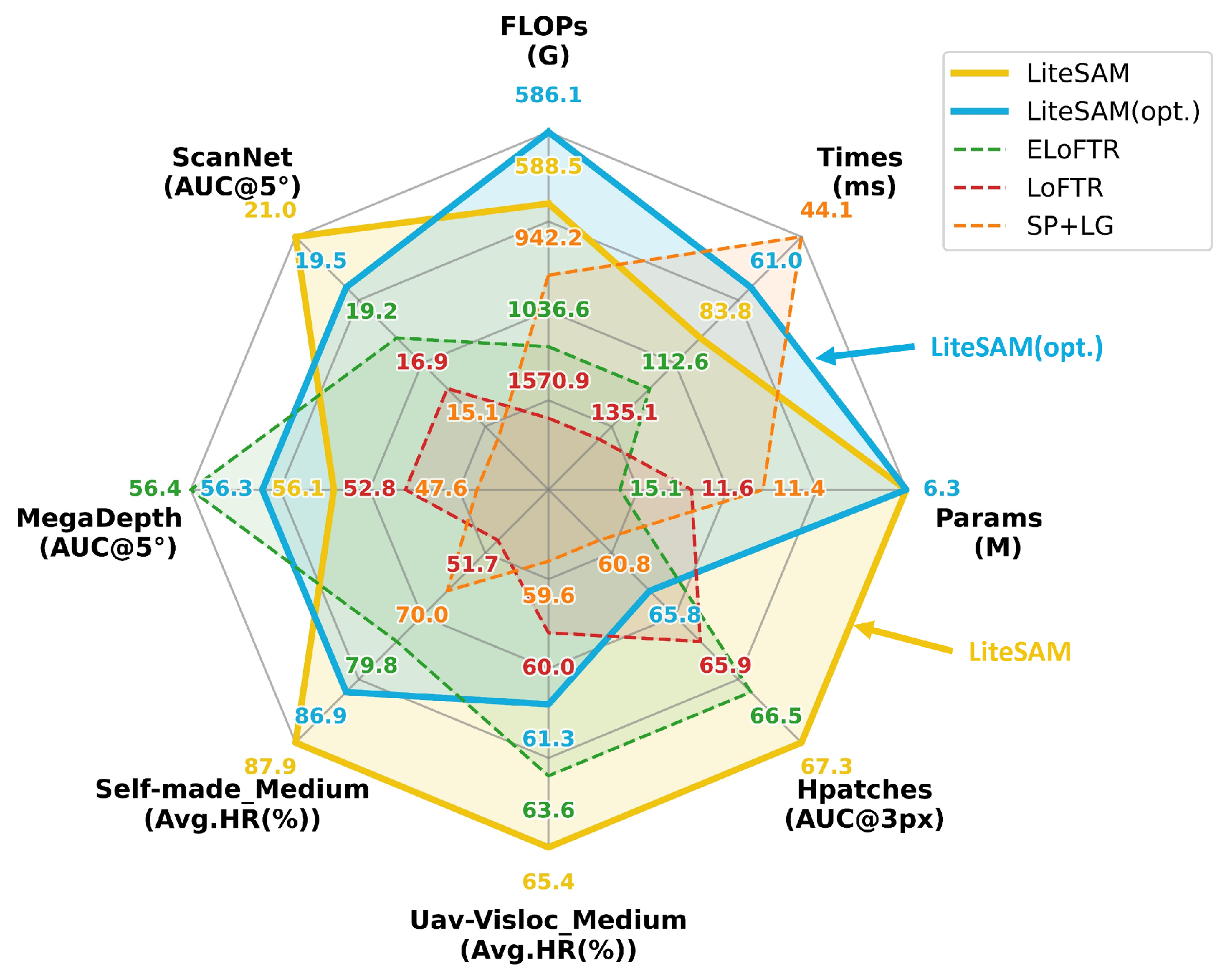
Comparing comprehensive performance of LiteSAM against other methods. The LiteSAM system exhibits a favorable accuracy–efficiency trade-off across both satellite–aerial datasets (self-made and Uav-Visloc [
19]) and natural image datasets (Hpatches [
20], MegaDepth [
21], and ScanNet [
22]) while maintaining significant advantages in computational efficiency and parameter size. SP+LG [
23,
24] achieves the fastest inference speed but at the expense of accuracy, whereas LoFTR [
15] and EffiicentLoFTR [
16] attain higher accuracy with substantially increased computational costs.
Figure 2.
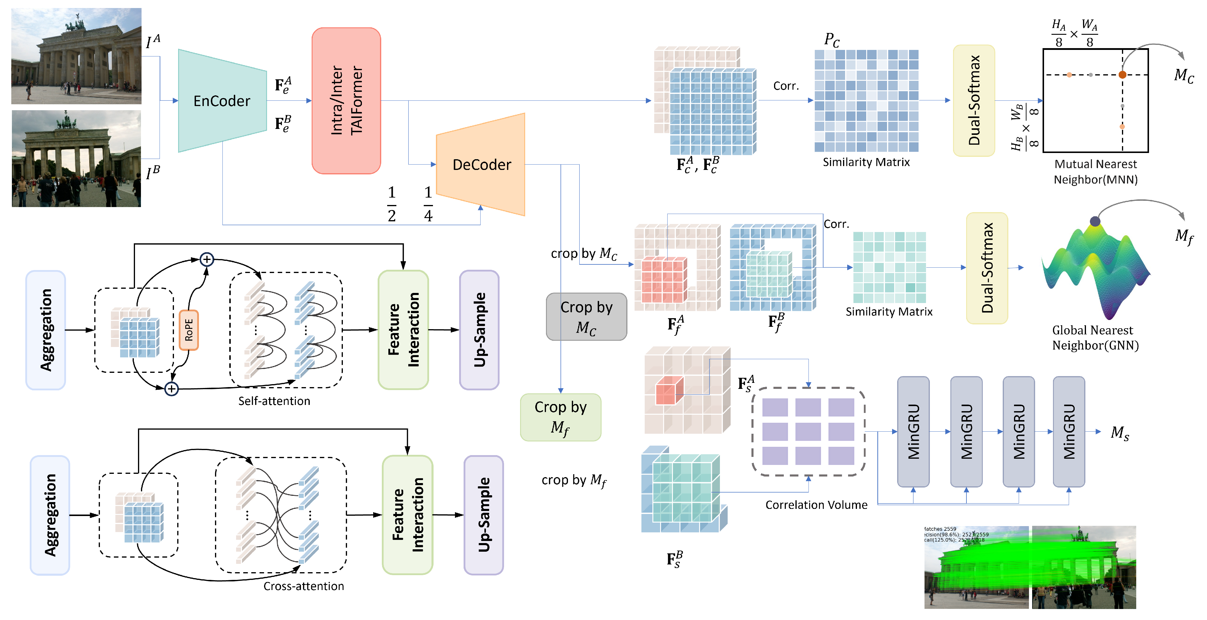
The framework of proposed LiteSAM: (1) image pair , is provided, and coarse features are extracted by the shared reparameterized network. (2) Feature interaction is then performed to enhance the discriminability of these features, yielding . (3) Coarse matching relationships are established to obtain initial matching . (4) Refinement process is applied to obtain pixel-level matching . (5) Finally, further refinement is conducted to achieve subpixel-level matching .
Figure 3.
Token Aggregation–Interaction Transformer (TAIFormer). Input features and are aggregated via convolution or max pooling to simplify computation. After this, local and global features are extracted and fused by the convolutional token mixer (CTM). Finally, the convolutional feed-forward network (ConvFFN) refines spatial structure and local context.
Figure 4.
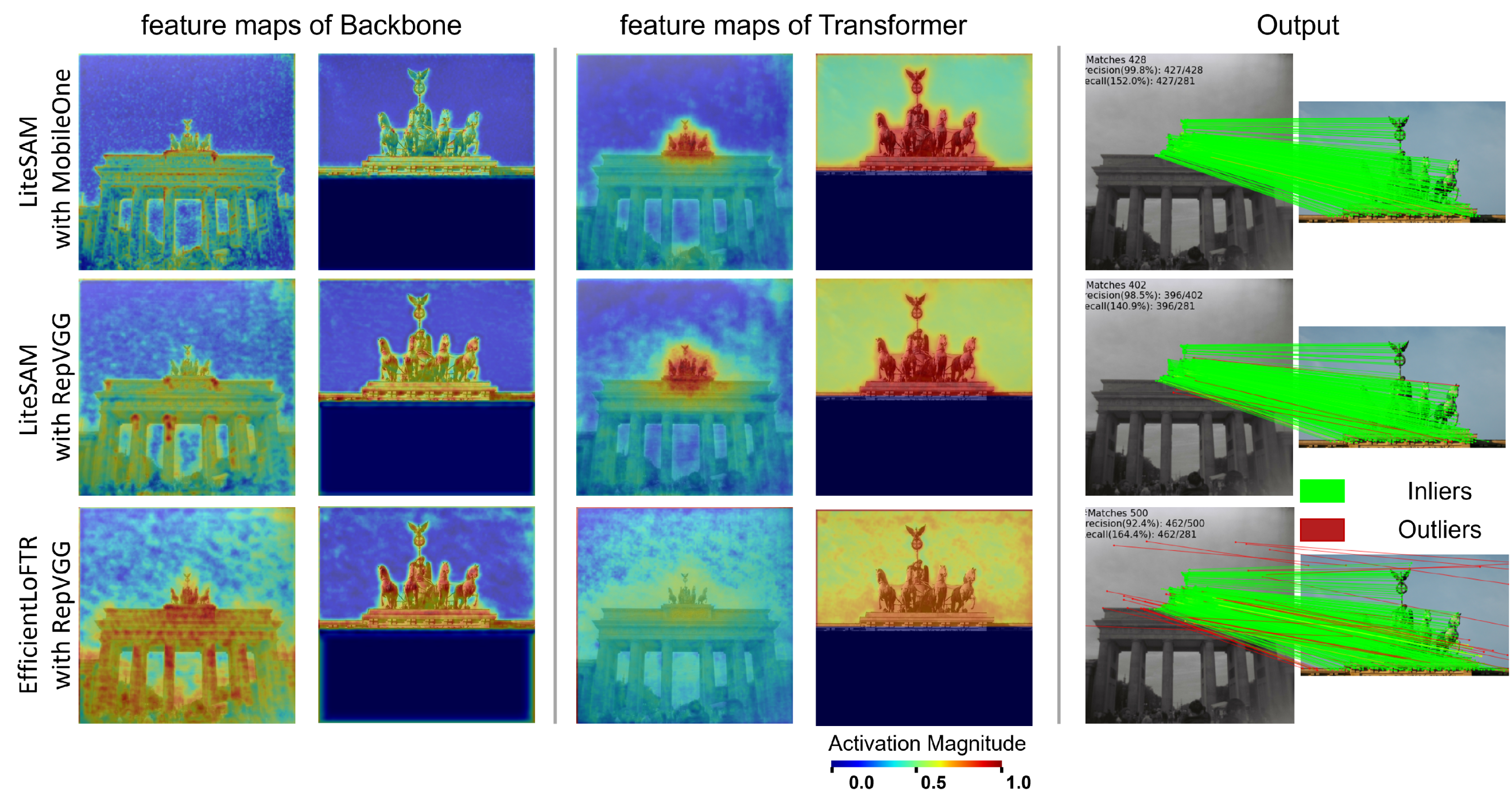
Feature visualization on the MegaDepth dataset. Feature maps are aggregated via L2 normalization across the channel dimension and rendered as heatmaps, where warmer hues (e.g., red) indicate higher activation magnitudes, reflecting greater model attention to corresponding regions. In the matching results, green lines denote inliers validated by an epipolar error threshold, while red lines indicate outliers.
Figure 5.
Learnable subpixel refinement module. A search window is centered at the matched point on the pixel-level feature map of the target image . A multi-layer MinGRU is utilized to iteratively refine the initial correspondence , achieving subpixel-level accuracy.
Figure 5.
Learnable subpixel refinement module. A search window is centered at the matched point on the pixel-level feature map of the target image . A multi-layer MinGRU is utilized to iteratively refine the initial correspondence , achieving subpixel-level accuracy.
Figure 6.
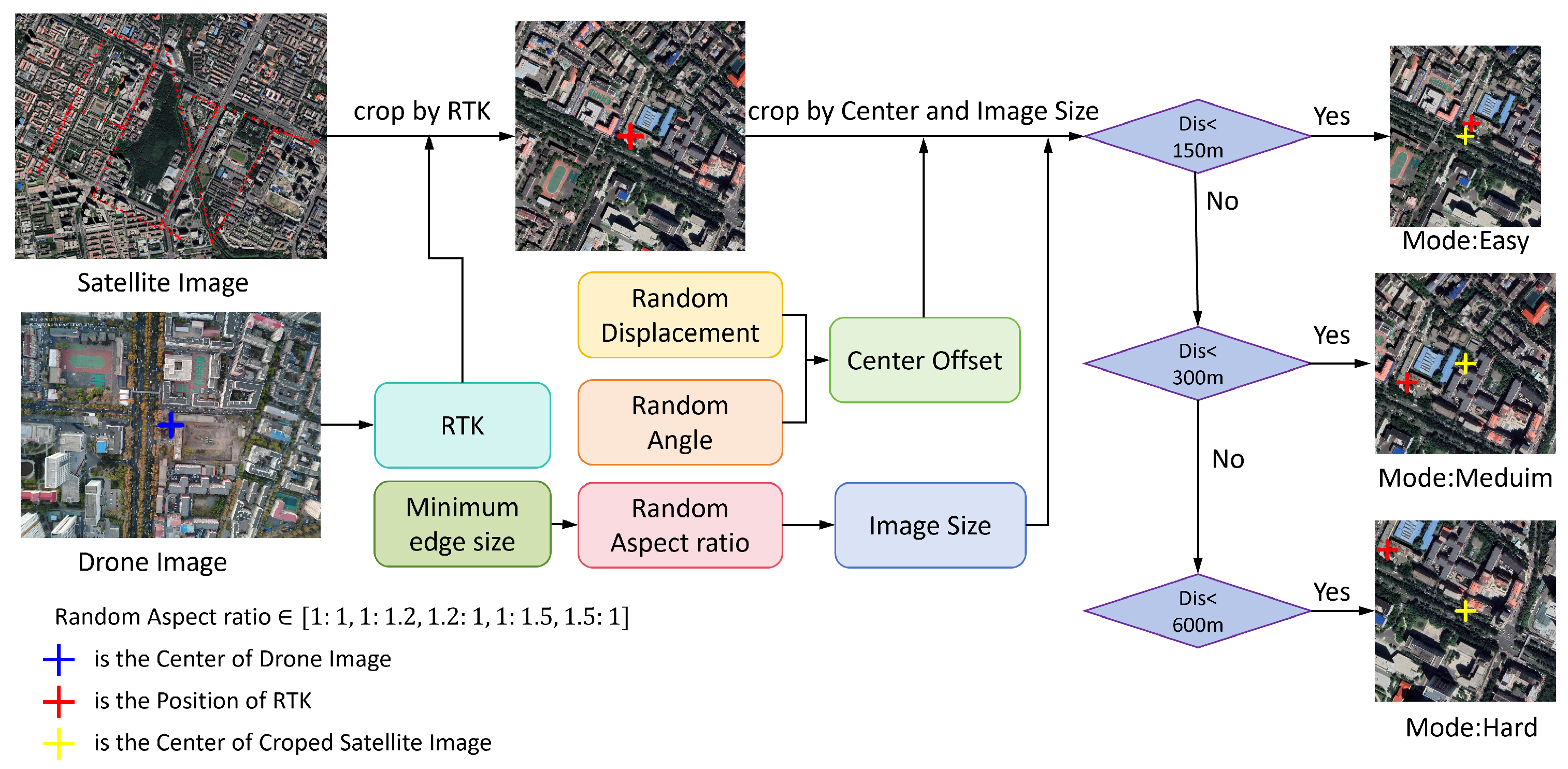
Dataset construction pipeline. UAV images are geolocated using high-precision RTK positioning, with coordinates serving as reference centers. Synthetic perturbations (easy: 0–150 m; moderate: 150–300 m; hard: 300–600 m) are applied to simulate varying localization difficulties. Images are cropped at multiple scales with a consistent 2000-pixel short edge to ensure scale uniformity.
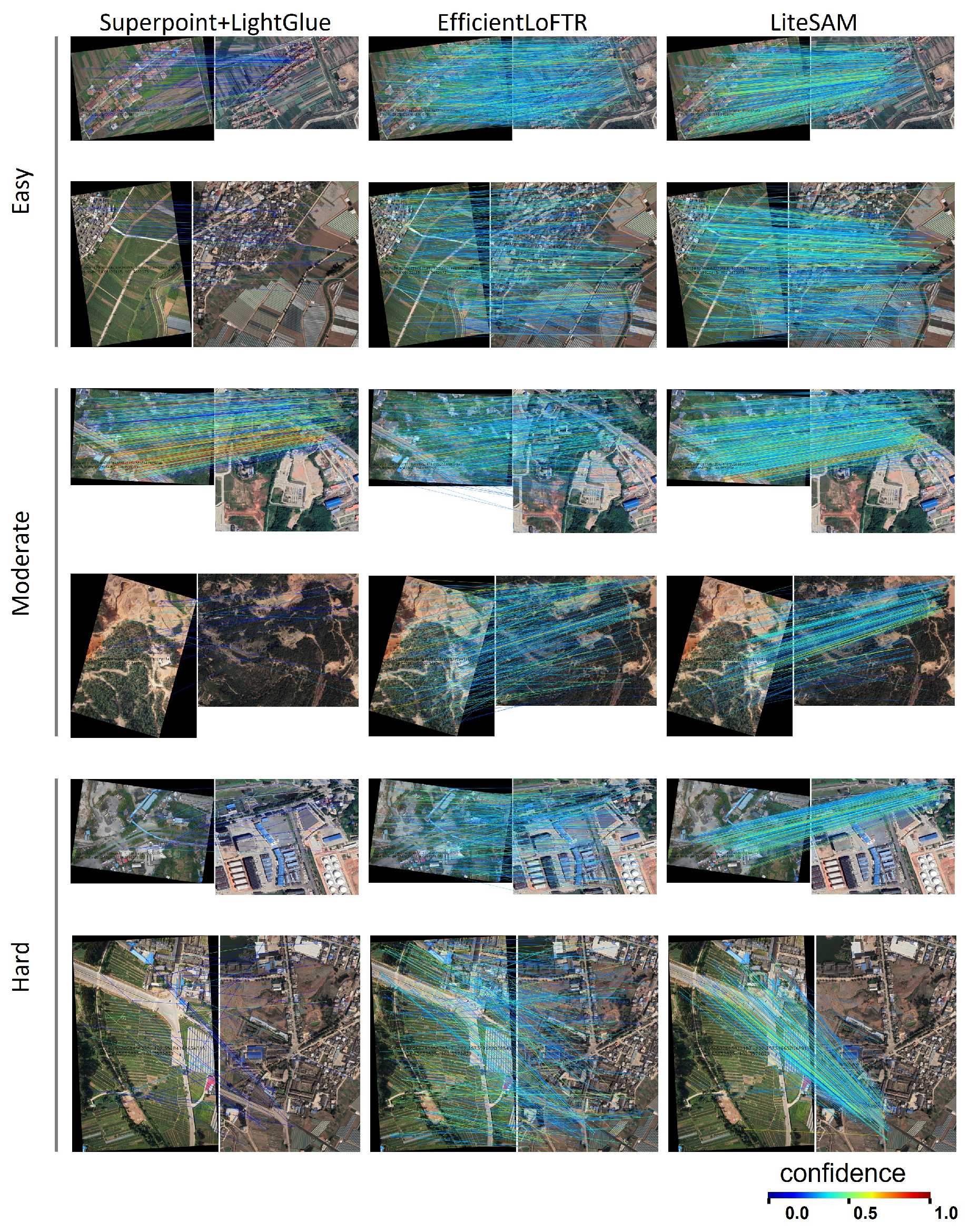
Figure 7.
Comparison of feature matching results on the UAV-VisLoc dataset. This figure presents the feature matching results of SuperPoint+LightGlue [
23,
24], EfficientLoFTR [
16], and LiteSAM on the UAV-VisLoc dataset [
19]. From left to right, the results correspond to SuperPoint+LightGlue, EfficientLoFTR, and LiteSAM, respectively, across varying difficulty levels. The figure is organized into three groups from top to bottom: the top two rows represent Easy Mode, the middle two rows represent Moderate Mode, and the bottom two rows represent Hard Mode.
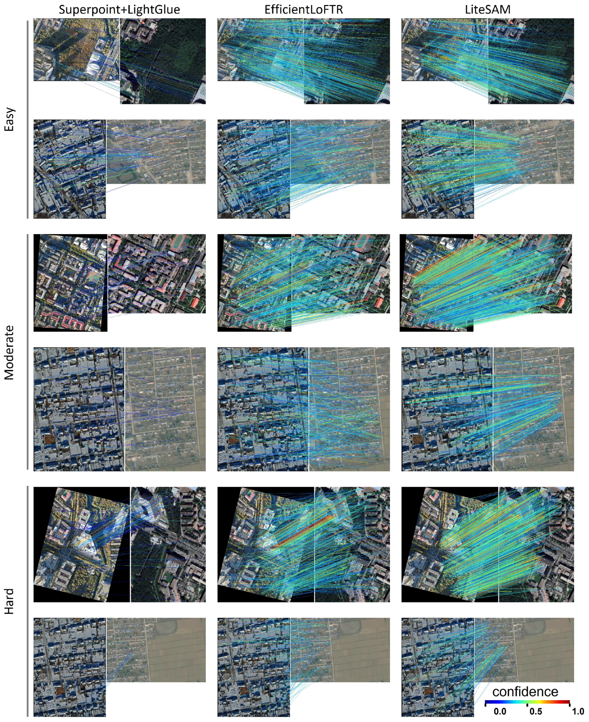
Figure 8.
Comparison of feature matching results on the self-made dataset. This figure presents the feature matching results of SuperPoint+LightGlue [
23,
24], EfficientLoFTR [
16], and LiteSAM on the self-made dataset. From left to right, the results correspond to SuperPoint+LightGlue, EfficientLoFTR, and LiteSAM, respectively, across varying difficulty levels. The figure is organized into three groups from top to bottom: the top two rows represent Easy Mode, the middle two rows represent Moderate Mode, and the bottom two rows represent Hard Mode.
Table 1.
Relative pose estimation results on MegaDepth and ScanNet. All models were trained solely on the MegaDepth dataset and evaluated across all benchmarks to assess generalization performance. Reported metrics include pose estimation errors at multiple thresholds and inference speeds on the MegaDepth dataset at an input resolution of pixels. In the semi-dense category, the best result is in red, the second-best is in orange, and the third-best is in blue. The direction indicated by the arrows denotes superior performance.
| Category | Method | MegaDepth | | ScanNet | Times (ms) |
|---|
|
AUC@5 |
AUC@10 |
AUC@20 | |
AUC@5 |
AUC@10 |
AUC@20 |
|---|
| Sparse | SP+SG | 42.2 | 61.2 | 76.0 | | 10.4 | 22.9 | 37.2 | 99.4 |
| SP+LG | 47.6 | 64.8 | 77.9 | | 15.1 | 32.6 | 61.02 | 47.1 |
| SP+OG | 47.4 | 65.0 | 77.8 | | 14.0 | 28.9 | 44.3 | 414.9 |
| Semi-Dense | LoFTR | 52.8 | 69.2 | 81.2 | | 16.9 | 33.6 | 50.6 | 314.82 |
| MatchFormer | 53.3 | 69.7 | 81.8 | | 15.8 | 32.0 | 48.0 | 691.0 |
| ASpanFormer | 55.3 | 71.5 | 83.1 | | 19.6 | 37.7 | 53.3 | 352.07 |
| TopicFM | 54.1 | 70.1 | 81.6 | | 17.3 | 35.5 | 50.9 | 270.69 |
| TopicFM+ | 58.2 | 72.8 | 83.2 | | 20.4 | 38.5 | 54.5 | 220.37 |
| RCM | 53.2 | 69.4 | 81.5 | | 17.3 | 34.6 | 52.1 | - |
| DeepMatcher | 55.7 | 72.2 | 83.4 | | - | - | - | - |
| EfficientLoFTR | 56.4 | 72.2 | 83.5 | | 19.2 | 37.0 | 53.6 | 154.2 |
| EfficientLoFTR (opt.) | 55.4 | 71.4 | 82.9 | | 17.4 | 34.4 | 51.2 | 98.8 |
| GeoAT | 53.6 | 70.3 | 82.2 | | - | - | - | - |
| ASpan_Homo | 57.1 | 73.0 | 84.1 | | 22.0 | 40.5 | 57.2 | >352 |
| LiteSAM | 56.1 | 72.0 | 83.4 | | 21.0 | 39.3 | 55.9 | 133.0 |
| LiteSAM (opt.) | 56.3 | 72.1 | 83.4 | | 19.5 | 37.8 | 54.7 | 79.9 |
| Dense | DKM | 60.4 | 74.9 | 85.1 | | 26.64 | 47.07 | 64.17 | 528.21 |
| ROMA | 62.6 | 76.7 | 86.3 | | 28.9 | 50.4 | 68.3 | 3336.22 |
Table 2.
Absolute visual localization results on the Aerial Image Dataset. All models were tested on images. The Percentage of Correct Keypoints (PCK), inference speed, FLOPs, and model parameters are shown. In the Semi-Dense category, the best result is in red, the second-best is in orange, and the third-best is in blue. The direction indicated by the arrows denotes superior performance.
| Category | Method | DeepAerial | Time (ms) | FLOPs (G) | Params (M) |
|---|
|
PCK@1% ↑
|
PCK@3% ↑
|
PCK@5% ↑
|
|---|
| Sparse | SP+NN | 11.5 | 19.0 | 23.2 | 9.53 | 44.46 | 1.3 |
| SP+SG | 8.4 | 16.5 | 19.8 | 66.85 | 108.13 | 13.32 |
| SP+LG | 21.4 | 27.0 | 29.3 | 43.74 | 91.62 | 11.38 |
| Semi-Dense | LoFTR | 18.5 | 24.8 | 28.1 | 52.74 | 308.73 | 11.56 |
| AspanFormer | 21.5 | 26.1 | 28.5 | 135.52 | 551.76 | 15.75 |
| EfficientLoFTR | 23.3 | 30.3 | 33.2 | 36.55 | 189.40 | 15.05 |
| EfficientLoFTR (opt.) | 21.4 | 29.9 | 32.8 | 32.08 | 189.28 | 15.05 |
| LiteSAM | 23.7 | 30.2 | 32.7 | 33.29 | 92.39 | 6.31 |
| LiteSAM (opt.) | 22.2 | 29.2 | 31.9 | 29.64 | 92.27 | 6.31 |
| Dense | DKM | 30.6 | 36.1 | 38.9 | 291.62 | 1543.86 | 70.21 |
| ROMA | 38.0 | 50.8 | 56.4 | 243.88 | 1864.42 | 111.29 |
Table 3.
Absolute visual localization results on UAV-VisLoc dataset. Metrics include RMSE under a 30 m threshold, average hit rate, number of matched points, and per-frame inference time across Easy, Moderate, and Hard settings. In the Semi-Dense category, the best result is in red, the second-best is in orange, and the third-best is in blue. The direction indicated by the arrows denotes superior performance.
| Category | Method | UAV-VisLoc Dataset (Easy/Moderate/Hard) | Time (ms) ↓ |
|---|
|
RMSE@30 ↓
| Avg.HR (%) ↑ |
Num of Point ↑
|
|---|
| Sparse | SP+NN | 18.71 | 37.15/29.54/19.89 | 819/820/804 | 19.82 |
| SP+SG | 17.88 | 58.38/56.64/51.03 | 454/378/251 | 138.27 |
| SP+LG | 17.81 | 60.34/59.57/54.32 | 473/402/276 | 44.15 |
| Semi-Dense | LoFTR | 17.99 | 59.96/59.96/50.59 | 548/422/254 | 135.09 |
| AspanFormer | 17.87 | 62.92/59.10/49.96 | 1368/887/556 | 159.16 |
| EfficientLoFTR | 17.87 | 65.78/63.62/57.65 | 1849/1483/971 | 112.60 |
| EfficientLoFTR (opt.) | 17.94 | 63.85/57.78/42.30 | 3873/3311/2639 | 77.53 |
| LiteSAM | 17.86 | 66.66/65.37/61.65 | 2096/1662/1065 | 83.79 |
| LiteSAM (opt.) | 17.98 | 65.09/61.34/46.16 | 4227/3587/2826 | 60.97 |
| Dense | DKM | 17.87 | 59.11/57.29/52.52 | 10,000/10,000/10,000 | 498.88 |
| ROMA | 17.81 | 64.13/60.67/52.70 | 10,000/10,000/10,000 | 688.32 |
Table 4.
Absolute visual localization results on self-made dataset. Results include RMSE within 30 m, average hit rate, number of correspondences, inference time, and FLOPs across varying difficulty levels. In the Semi-Dense category, the best result is in red, the second-best is in orange, and the third-best is in blue. The direction indicated by the arrows denotes superior performance.
| Category | Method | Self-Made Dataset (Easy/Moderate/Hard) | Time (ms) | FLOPs (G) |
|---|
|
RMSE@30 ↓
|
Avg.HR (%) ↑
|
Num of Point
|
|---|
| Sparse | SP+NN | 13.26 | 30.27/21.37/14.08 | 1123/1103/1071 | 20.64 | 148.7 |
| SP+SG | 5.70 | 71.28/64.96/54.78 | 492/371/233 | 142.28 | 967.9 |
| SP+LG | 6.76 | 78.85/70.03/58.31 | 622/482/322 | 49.49 | 942.16 |
| Semi-Dense | LoFTR | 8.74 | 63.03/51.71/41.09 | 288/147/87 | 145.61 | 1570.92 |
| AspanFormer | 7.93 | 73.52/59.85/42.03 | 863/515/272 | 163.45 | 1738.81 |
| EfficientLoFTR | 7.28 | 90.03/79.79/61.84 | 1540/1114/728 | 120.72 | 1036.61 |
| EfficientLoFTR (opt.) | 8.43 | 88.95/75.84/54.17 | 4526/3953/3382 | 80.34 | 1033.54 |
| LiteSAM | 6.12 | 92.09/87.88/77.30 | 1905/1406/888 | 85.31 | 588.51 |
| LiteSAM (opt.) | 6.89 | 92.34/86.93/72.10 | 4356/3743/3128 | 61.98 | 586.06 |
| Dense | DKM | 5.86 | 77.09/75.15/71.06 | 10,000/10,000/10,000 | 512.71 | 3022.67 |
| ROMA | 5.60 | 92.00/86.11/76.10 | 10,000/10,000/10,000 | 691.48 | 6750.08 |
Table 5.
Visual localization results on the Aachen Day-Night v1.1 and InLoc datasets. The visual localization performance is evaluated on the Aachen Day-Night v1.1 [
48] and InLoc [
49] datasets using the HLoc framework [
59]. In the Semi-Dense category, the best result is in
red, the second-best is in
orange, and the third-best is in
blue. The direction indicated by the arrows denotes superior performance.
| Category | Method | AachenV1.1 | | Inloc |
|---|
|
Day
|
Night
| |
DUC1
|
DUC2
|
|---|
|
(0.25 m, 2°)/(0.5 m, 5°)/(1.0 m, 10°)
| |
(0.25 m, 2°)/(0.5 m, 5°)/(1.0 m, 10°)
|
|---|
| Sparse | SP+SG | 89.8/96.1/99.4 | 77.0/90.6/100.0 | | 49.0/68.7/80.8 | 53.4/77.1/82.4 |
| SP+LG | 89.2/95.4/98.5 | 87.8/93.9/100.0 | | 49.0/68.2/79.3 | 55.0/74.8/79.4 |
| Semi-Dense | LoFTR | 88.7/95.6/99.0 | 78.5/91.1/99.0 | | 47.5/72.2/85.5 | 54.2/74.8/85.5 |
| MatchFormer | - | - | | 46.5/73.2/85.9 | 55.7/71.8/85.5 |
| ASpanFormer | 89.4/95.6/99.0 | 77.5/91.6/99.5 | | 51.5/73.7/86.4 | 55.0/74.0/85.5 |
| TopicFM | 90.2/95.9/98.9 | 77.5/91.1/99.5 | | 52.0/74.7/87.4 | 53.4/74.8/83.2 |
| RCM | 89.7/96.0/98.7 | 72.8/91.6/99.0 | | - | - |
| SAM | 89.7/95.8/99.0 | 78.6/91.8/100.0 | | 51.8/73.9/87.8 | 56.0/75.8/83.1 |
| EfficientLoFTR | 89.6/96.2/99.0 | 77.0/91.1/99.5 | | 52.0/74.7/86.9 | 58.0/80.9/89.3 |
| LiteSAM | 88.6/96.0/98.8 | 76.4/91.1/99.5 | | 52.0/73.7/86.4 | 60.3/85.5/89.3 |
| LiteSAM (opt.) | 88.6/95.5/98.8 | 76.4/90.6/99.5 | | 54.0/74.2/86.9 | 55.7/80.9/85.5 |
| Dense | DKM | - | - | | 51.5/75.3/86.9 | 63.4/82.4/87.8 |
| ROMA | - | - | | 60.6/79.3/89.9 | 66.4/83.2/87.8 |
Table 6.
Homography estimation results on the HPatches dataset. Performance comparison of feature matching methods based on the percentage of image pairs with average corner error below predefined pixel thresholds. All images are resized to 480 pixels (short side), and homographies are estimated from 1000 correspondences using an RANSAC-based solver. In the Semi-Dense category, the best result is in red, the second-best is in orange, and the third-best is in blue. Methods marked with † are tested under the same experimental conditions as LiteSAM for a fair comparison. The direction indicated by the arrows denotes superior performance.
| Category | Method | Homography est. AUC |
|---|
| @3 px↑ | @5 px↑ | @10 px↑ |
|---|
| Sparse | D2Net+NN | 23.2 | 35.9 | 53.6 |
| R2D2+NN | 50.6 | 63.9 | 76.8 |
| DISK+NN | 52.3 | 64.9 | 78.9 |
| SP+SG | 53.9 | 68.3 | 81.7 |
| SP+LG † | 60.8 | 72.3 | 84.0 |
| Semi-Dense | Sparse-NCNet | 48.9 | 54.2 | 67.1 |
| DRC-Net | 50.6 | 56.2 | 68.3 |
| LoFTR | 65.9 | 75.6 | 84.6 |
| EfficientLoFTR | 66.5 | 76.4 | 85.5 |
| EfficientLoFTR (opt.) † | 65.1 | 75.2 | 84.8 |
| AspanFormer | 67.4 | 76.9 | 85.6 |
| TopicM | 67.3 | 77.0 | 85.7 |
| GeoAT | 69.1 | 78.2 | 87.1 |
| ASpan_Homo | 70.2 | 79.6 | 87.8 |
| JamMa | 68.1 | 77.0 | 85.4 |
| LiteSAM | 67.3 | 77.2 | 86.1 |
| LiteSAM (opt.) | 65.8 | 76.2 | 85.6 |
| Dense | DKM | 71.3 | 80.6 | 88.5 |
| Pmatch | 71.9 | 80.7 | 88.5 |
Table 7.
Ablation study on self-made dataset. AVL performance on the self-made dataset, reported in terms of RMSE@30m, average hit rate, number of correspondences, inference time, and computational cost (FLOPs) across different architectural variants of LiteSAM. The best result is in red, the second-best is in orange, and the third-best is in blue. The direction indicated by the arrows denotes superior performance.
| Method | Self-Made Dataset(Easy/Moderate/Hard) | FLOPs (G) | Time (ms) |
|---|
| RMSE@30 ↓ | Avg.HR (%) ↑ |
Num of Point
|
|---|
| Full | 6.12 | 92.09/87.88/77.30 | 1905/1406/888 | 588.51 | 85.31 |
| (1) Replace MobileOne with RepVGG | 6.46 | 92.95/89.81/79.53 | 1520/1132/756 | 1066.24 | 100.77 |
| (2) Replace TAIFormer to Agg. Attention | 6.94 | 89.68/81.38/63.99 | 1477/1091/727 | 697.11 | 99.72 |
| (3) Replace MinGRU to heatmap refine | 6.39 | 91.75/86.67/73.45 | 1759/1317/859 | 588.49 | 86.49 |
| (4) Remove MinGRU refinement | 6.47 | 90.14/83.71/70.49 | 1864/1385/867 | 588.49 | 83.94 |
| (5) Our Optimal (w/o dual softmax) | 6.89 | 92.34/86.93/72.10 | 4356/3743/3128 | 586.06 | 61.98 |
Table 8.
Ablation study on MegaDepth dataset. Relative pose estimation performance of LiteSAM variants, trained and tested on MegaDepth at resolution, reporting pose estimation AUC and inference times. The best result is in red, the second-best is in orange, and the third-best is in blue. The direction indicated by the arrows denotes superior performance.
| Method | Pose Estimation AUC | Times (ms) |
|---|
|
AUC@5° ↑
|
AUC@10° ↑
|
AUC@20° ↑
|
|---|
| Full | 56.1 | 72.0 | 83.4 | 133.0 |
| (1) Replace MobileOne with RepVGG | 55.7 | 71.8 | 83.3 | 147.8 |
| (2) Replace MobileOne with ResNet | 55.4 | 71.7 | 83.2 | 162.4 |
| (3) Replace TAIFormer to Agg. Attention | 55.0 | 71.1 | 82.7 | 141.4 |
| (4) Replace MinGRU to heatmap refine | 55.6 | 71.9 | 83.4 | 133.4 |
| (5) Remove MinGRU refinement | 55.4 | 71.6 | 83.2 | 131.4 |
| (6) Our Optimal (w/o dual softmax) | 56.3 | 72.1 | 83.4 | 79.9 |
Table 9.
Impact of jmage resolution on localization performance on the MegaDepth dataset. AUC of pose estimation and inference time for LiteSAM (original) with dual softmax and LiteSAM (opt.) without dual softmax. The best result is in red, the second-best is in orange, and the third-best is in blue. The direction indicated by the arrows denotes superior performance.
| Resolution | Dual Softmax | Pose Estimation AUC | Prec ↑ | Num of Points | Times (ms) |
|---|
|
AUC@5° ↑
|
AUC@10° ↑
|
AUC@20° ↑
|
|---|
| 640 × 640 | ✓ | 50.7 | 67.5 | 79.9 | 97.8 | 1068.6 | 38.9 |
| - | 50.7 | 67.5 | 79.9 | 96.6 | 1085.6 | 30.7 |
| 800 × 800 | ✓ | 53.2 | 69.9 | 81.9 | 98.0 | 1639.2 | 55.7 |
| - | 53.5 | 69.8 | 81.7 | 96.7 | 1682.3 | 38.2 |
| 960 × 960 | ✓ | 55.0 | 71.1 | 82.9 | 98.2 | 2320.3 | 77.5 |
| - | 55.3 | 71.3 | 82.9 | 96.7 | 2403.7 | 50.1 |
| 1184 × 1184 | ✓ | 56.1 | 72.0 | 83.4 | 98.0 | 3449.3 | 133.0 |
| - | 56.3 | 72.1 | 83.4 | 96.1 | 3619.0 | 79.9 |
| 1408 × 1408 | ✓ | 56.3 | 72.4 | 83.9 | 98.0 | 4765.3 | 227.5 |
| - | 56.8 | 72.6 | 83.9 | 95.5 | 5065.1 | 132.5 |
Table 10.
Localization performance on the self-made dataset using NVIDIA Jetson AGX Orin. Results include RMSE within 30 m, average hit rate, number of correspondences, and inference time across difficulty levels. The best result is in red, the second-best is in orange, and the third-best is in blue. The direction indicated by the arrows denotes superior performance.
| Method | Self-Made Dataset (Easy/Moderate/Hard) | Time (ms) |
|---|
|
RMSE@30 ↓
|
Avg.HR (%) ↑
|
Num of Point
|
|---|
| EfficientLoFTR | 7.53 | 90.76/78.63/59.24 | 2443/2011/1620 | 758.84 |
| EfficientLoFTR (opt.) | 8.31 | 88.87/75.67/53.44 | 4572/4011/3492 | 620.67 |
| LiteSAM | 6.17 | 92.69/89.08/77.21 | 2691/2113/1578 | 600.37 |
| LiteSAM (opt.) | 6.72 | 92.48/86.20/72.23 | 4388/3821/3220 | 497.49 |
