A Domain Adaptation-Based Ocean Mesoscale Eddy Detection Method Under Harsh Sea States

Highlights

What are the main findings?

• A framework integrating large kernel convolution with an adversarial domain adaptation framework was developed to specifically target mesoscale eddy detection in harsh sea states.
• The proposed method outperforms existing state-of-the-art methods, achieving a 7.2% improvement in Mean Intersection over Union (mIoU) on a specialized dataset simulating harsh sea conditions.

What is the implication of the main finding?

• The problem of eddy detection in harsh sea states can be effectively framed as a cross-domain challenge, validating the use of domain adaptation as a solution.
• The improved performance provides a more robust and reliable tool for automated eddy analysis, especially under the influence of extreme weather events.

Abstract

Under harsh sea states, the dynamic characteristics of ocean mesoscale eddies (OMEs) become significantly more complex, posing substantial challenges to their accurate detection and identification. In this study, we propose an artificial intelligence detection method for OMEs based on the domain adaptation technique to accurately perform pixel-level segmentation and ensure its effectiveness under harsh sea states. The proposed model (LCNN) utilizes large kernel convolution to increase the model’s receptive field and deeply extract eddy features. To deal with the pronounced cross-domain distribution shifts induced by harsh sea states, an adversarial learning framework (ADF) is introduced into LCNN to enforce feature alignment between the source (normal sea states) and target (harsh sea states) domains, which can also significantly improve the segmentation performance in our constructed dataset. The proposed model achieves an accuracy, precision, and Mean Intersection over Union of 1.5%, 6.0%, and 7.2%, respectively, outperforming the existing state-of-the-art technologies.

1. Introduction

Detecting the crucial ocean mesoscale eddies (OMEs) under harsh sea states, characterized by conditions such as significant wave heights (SWHs) exceeding 4 m and surface wind speeds surpassing 17 m/s, is of great significance but faces numerous challenges. Such conditions are commonly accompanied by significant fluctuations of SSH, anomalous distributions of sea surface temperature (SST), and intense activities of ocean surface currents, all of which are often further modulated by eddies [1,2]. Conversely, these extreme sea states can significantly alter the dynamic behaviors of eddies [3]. For example, intense wind stress induced by typhoons could lead to rapid changes in the morphology and position of eddies and even the formation of secondary eddies [4]. Moreover, the strong noise occurring under harsh sea states, such as storm surges and surface waves, poses more complexity to the OME detection based on remote sensing data or numerical simulations. The OME detection under harsh sea states is essential for understanding the interactions among typhoons, waves, and oceans. Moreover, it provides scientific support for maritime safety, extreme weather prevention, and disaster warning systems. Despite its crucial importance, reliable OME detection under such conditions remains a significant technical challenge. To our knowledge, the majority of research has focused on developing detection methods for normal sea states, where signals are clearer and less affected by noise.

Generally, detecting OMEs can be regarded as marking the regions where OMEs occur in an image. In earlier years, traditional methods for OME detection relied on manual annotations, mathematical or physical knowledge, and image processing techniques [5]. With the increase in ocean observation data and advancements in computational power, deep learning has gradually shown unique advantages in OME detection. Despite this progress, dealing with the interference induced by harsh sea states on the ocean surface and data collection remains challenging.

Traditional Detection Methods: The most widely used physics-based method is the Okubo–Weiss (OW) parameter method [6,7], which introduced a parameter to describe eddy activities in a flow field. It calculated the shear and rotational strain to describe the dynamic characteristics of the flow. The OW parameter method strongly depended on the choice of threshold and experience, which often resulted in substantial misclassifications. The Winding-Angle (WA) [8] algorithm and Vector Geometry (VG) [9,10] algorithm did not rely on parameter selection, but they focused on the global topological properties of the flow field for OME detection instead. Later, an automatic eddy detection method based on the SSH data [11,12,13] from satellite altimeters emerged as a more accurate, threshold-free eddy detection technique; however, it was susceptible to the strong noise in the flow field, leading to misclassifications. Therefore, the traditional physics-based approaches either relied on the choice of parameters and experience or struggled to generalize in complex oceanic states, motivating the exploration of AI-based methods for more robust and adaptive OME detection.

Deep Learning-based Research: Referring to previous studies, detecting OMEs can be typically defined as a semantic segmentation task [14]. For instance, Lguensat et al. [15] proposed the EddyNet approach, a U-Net-based semantic segmentation architecture that used SSH data for pixel-level eddy classification. Subsequently, Du et al. [16] proposed DeepEddy to implement the classification of SAR images, which combined the Principal Component Analysis Network [17] with Spatial Pyramid Pooling. Xu et al. applied PSPNet [18], a semantic segmentation architecture, for OME detection. Duo et al. [19] applied bounding boxes for OME detection based on SLA data, focusing on object detection rather than pixel-level classification to obtain accurate eddy localization. DeepLabV3 [20] employed Atrous Spatial Pyramid Pooling (ASPP) to integrate contextual information and employed parallel atrous convolutions with varying dilation rates to extract multiscale features. Zhao et al. [21] utilized Pyramid Split Attention (PSA) U-Net to extract OMEs from remote sensing images. PSA_EDUNet [21], based on the UNet architecture, incorporated the PSA module and skip connections to capture eddy spatial information at different scales from both channel and spatial attention perspectives. DUNet [22] adopted a dual encoder–decoder structure to mitigate the issue of overfitting in deep learning models. In recent work, Ding et al. [23] established four foundational design principles for large kernel convolutional networks, ConvNets, systematically revealing their potential across various new domains. In the architecture, a larger receptive field enabled the simultaneous capture of multiscale contextual features, which facilitated enhanced learning of eddy structures characterized by intricate spatial patterns and localized morphological details. It helped the model better understand the relationship between the global structure and local variations in complex sea surface environments. However, most existing deep learning models were trained in relatively stable meteorological or ocean conditions (i.e., calm or light sea states). It creates a significant domain shift when the models are applied to real-world scenarios involving extreme weather. This shift severely restricts the models’ generalization ability. Specifically, the visual characteristics of eddies and the surrounding sea surface states change dramatically under high-noise conditions, preventing models from extracting robust and valid features and thereby leading to a rising rate of false detections. Therefore, bridging this domain gap is essential for developing a truly reliable OME detection system, which necessitates the introduction of domain adaptation strategies.

Domain adaptation aims to transfer knowledge acquired from a source domain to a target domain [24]. The knowledge from each domain contains similar objects but exhibits different data distributions. In many practical scenarios, training data come from a source domain that is well-annotated but exhibits a domain shift from the real-world target domain, which typically has scarce or even no annotations. In this view, if conceptualizing the essence of harsh sea states as specific modes of ocean dynamics, we can frame the harsh sea states problem as a cross-domain challenge. We take normal sea states as the source domain and harsh sea states as the target domain. However, directly applying a model trained on the source domain to the target domain often results in substantial performance degradation. Domain adaptation addresses this issue by establishing a mechanism to mitigate the distribution discrepancy between the source and target domains, thereby enhancing the model’s generalization ability on the target domain. Depending on the availability of labeled data in the target domain, domain adaptation methods can be categorized into supervised, self-supervised, semi-supervised, and unsupervised approaches. Among them, Unsupervised Domain Adaptation (UDA) is the most challenging [25], as it relies solely on labeled data from the source domain and unlabeled data from the target domain during training. Recently, this technique has been extensively applied to semantic segmentation tasks [26,27,28]. Adversarial training is one of the UDA methods designed to align the distributions of the source and target domains at feature and output levels within a Generative Adversarial Network (GAN) framework. Using multiscale or multi-category information as discriminators can refine the alignment process. Inspired by this, we develop an eddy segmentation architecture which incorporates an ADF to ensure an effective OME segmentation under harsh sea states.

Specific Contributions of Our Work:

• Investigating changes in sea surface data under harsh sea states: We have developed a dataset for OME detection, including sea level anomaly (SLA) data in normal sea states, which we constructed based on the reanalysis dataset of the South China Sea (REDOS) [29], and SLA data in the harsh sea states obtained using a two-dimensional (2D) Gaussian function (GF), along with corresponding annotations.
• Introducing an adversarial learning framework (ADF): We conceptualize the essence of harsh sea states as specific modes of ocean variabilities, thereby framing the harsh sea states problem as a cross-domain challenge. Thus, the domain adaptation technique can be applied to obtain promising results in both normal and harsh sea states. By incorporating a domain discrimination module, we introduce an ADF to learn domain-invariant feature representations between source (normal sea states) and target (harsh sea states) domains. It effectively addresses the challenges of abnormal sea surface disturbances and substantial background noise under harsh sea states. The proposed method achieves superior performance based on harsh sea states datasets compared to models without the domain discriminator module.
• Proposing a novel end-to-end eddy segmentation model with large kernel convolution (LCNN): This model utilizes large kernel convolution to systematically expand the effective receptive field of the model and increase the level of spatial abstraction. It contributes to coping with complex fluctuations and various irregular eddy forms on the sea surface in harsh sea states. It also introduces more learnable parameters and nonlinear elements to increase the model’s representation capacity.

2. Proposed Method

Adversarial Domain Adaptation is a method that leverages adversarial learning mechanisms to enable a model to learn domain-invariant feature representations between the source (normal sea states) and target (harsh sea states) domains, thereby achieving cross-domain knowledge transfer. This architecture integrates a domain discrimination module with a Gradient Reversal Layer, and the gradient from the domain discriminator can be reversed and propagated back to the model. It inhibits the domain discriminator from identifying the different data sources, which encourages the model to extract the domain-invariant features that are indistinguishable between the source and target domains. Ultimately, adversarial training prompts the model to obtain similar feature representations and outputs in both domains, which improves the model’s generalization ability on the target domain and ensures its detection effectiveness under harsh sea states. We leverage this mechanism to design our training approach.

Our approach defines a source domain S to describe ocean dynamics in normal sea states and a target domain H to stand for the variabilities in harsh sea states. The source domain is derived from the SLA dataset we constructed based on the REDOS [29] in normal sea states, while the target domain is a processed REDOS dataset with SLA under harsh sea states obtained using a 2D GF. Although sharing similar underlying data structures (i.e., maritime region, data types), the source and target domains exhibit distinct distribution characteristics of data. Therefore, the proposed method consists of two distinguishable modules: a domain discriminator and a segmentation model LCNN. Adversarial learning employs a domain discriminator to align LCNN’s output distributions between source and target domains, thereby achieving domain adaptation from S to H. Figure 1 illustrates the complete architecture of the proposed method.

Below, we detail the modules and strategies involved in our method.

LCNN: The encoder–decoder architecture has been proven effective for eddy segmentation in various studies. Based on this framework, we develop an eddy segmentation architecture with an ADF, which is referred to as LCNN in this study. The proposed model consists of an attention module, encoder, pyramid pooling module, decoder, 1 × 1 convolution, and a softmax activation function. It progressively encodes the high-dimensional features of the input data, decodes them to restore the segmentation results, and ensures that the model can not only extract deep features of OMEs but also output accurate pixel-level OME masks at high resolution. An attention module is applied to extract spatial weights, enhance the ability to focus on local features in harsh sea states, and avoid false or missed detections caused by strong noise or disturbance. Finally, the 1 × 1 convolution is adopted to merge channels, and the softmax activation function is applied to obtain the segmentation result for each pixel.

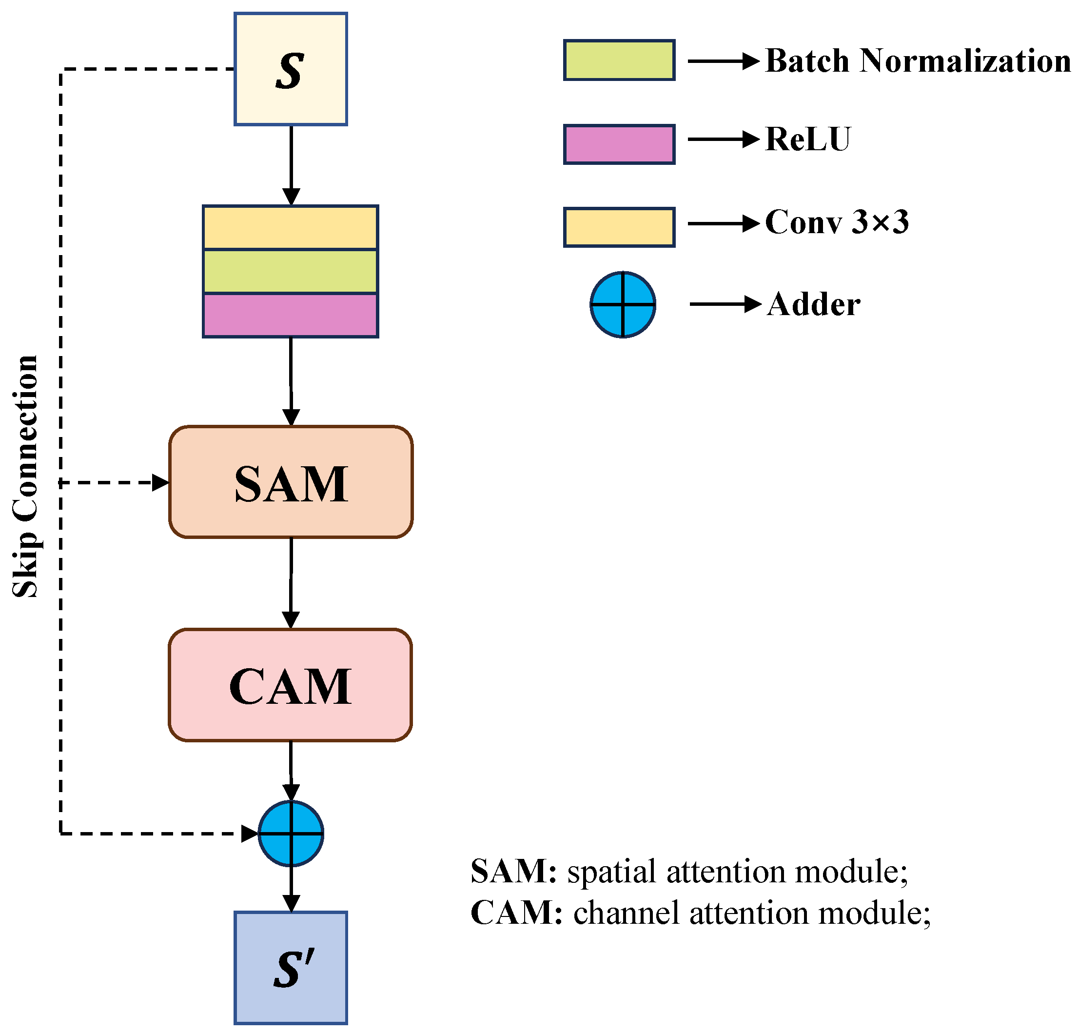
Attention Module: Figure 2 illustrates the overall structure of the attention module, which is composed of convolutional layers, residual connections (also called skip connections), spatial attention modules (SAMs), and channel attention modules (CAMs). Ahead of the attention block, a 3 × 3 convolutional layer is adopted to convert the original input into a C-channel feature map, where C is a hyperparameter of the architecture.

SAM: A spatial multi-head attention mechanism was involved in the SAM. As shown in Figure 3, it constructs multiple parallel attention matrices from the feature mappings of the convolutional block, revealing pixel relationships in the spatial domain. To construct the attention matrices, an input feature map is projected into Query (Q), Key (K), and Value (V) tensors using three independent $3\times 3$ convolutional layers, making the projections spatially context-aware. The Q, K, and V tensors are then split into multiple parallel heads H (Mul in Figure 3). Critically, unlike standard spatial attention, our mechanism calculates attention across the feature dimensions within [30] each head, thereby modeling the intercorrelations of the learned features. The outputs from all heads are concatenated, fused via a final convolutional layer, and then integrated back using a residual connection. In our implementation, we set the number of heads H to 8 and the hidden feature dimension to 128. The spatial attention is applied to the original pixel matrices through element-wise multiplication, enabling the model to measure similarity among input elements. This process assigns varying levels of importance to each input, which allows the model to focus on the most pertinent information. The multi-head self-attention mechanism captures spatial attention representations by applying weighting within individual channels, and the convolutional layers primarily operate on the spatial dimension, extracting local features and spatial patterns. It is crucial to detecting eddy boundaries, rotation directions, and SSH anomalies in the eddy core region, covering both the local and overall eddy structures.

CAM: Each channel is generally considered an independent feature map, and this independence assumption prevents the model from capturing the relationships between various channels. Different channels commonly carry information with different characteristics. The ability of the CAM to enhance or suppress certain features helps to extract significant representations more effectively.

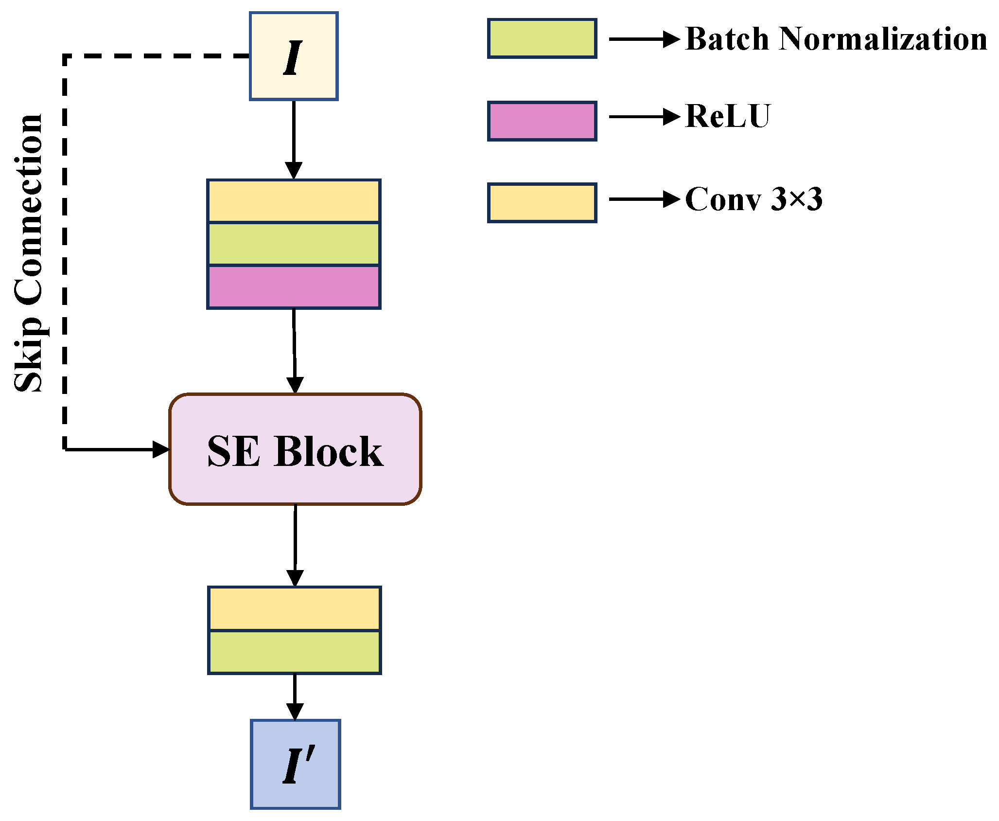
Our proposed CAM, illustrated in Figure 4, is implemented as a sophisticated residual block integrated with a channel attention mechanism. Specifically, for a given input feature map, the module first processes it through a primary path containing a 3 × 3 convolution, a Rectified Linear Unit (ReLU) activation, which introduces nonlinearity into the model by setting all negative values to zero, and a Batch Normalization layer. In parallel, a shortcut connection processes the original input through a projection layer (a 1 × 1 convolution) to match feature dimensions. The outputs of the primary path and the shortcut are then fused via element-wise addition. This fused feature map is subsequently fed into a Squeeze-and-Excitation (SE) block [31] for dynamically determining the weights for each channel. The SE block first applies global average pooling to ‘squeeze’ spatial information. Then, an ‘excitation’ step applies a two-layer fully connected network to learn channel-wise relationships. Crucially, this network employs a bottleneck architecture with a reduction ratio $r=16$. Finally, a 1 × 1 convolution maps the re-weighted features to the desired number of output channels.

With the incorporation of this composite CAM structure, the model can autonomously assign weights to different channels, optimize feature extraction more efficiently, enhance the importance of eddy-related features, and reduce the interference of strong wind-induced background flow. It leads to more precise and reliable eddy segmentation under harsh sea states. Figure 4 illustrates the CAM proposed in this study.

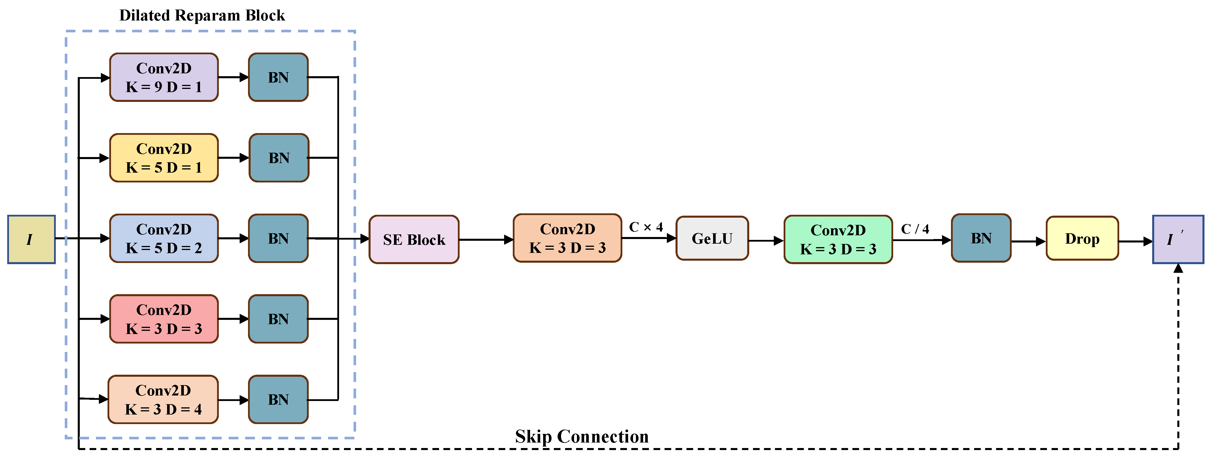
Encoder: The encoder is composed of a stacked feature extraction module (FEM). As shown in Figure 5, a FEM usually consists of a Dilated Reparam Block, an SE Block, and a feedforward neural network. The Dilated Reparam Block (DRB) proposed by Ding et al. [23] consists of five parallel dilated convolutions and batch normalization layers. From a parameter perspective, the dilated layer function is similar to a standard convolutional layer but with a large, sparsely populated kernel. The entire DRB is a large kernel convolution (LKC) operator. In recent research, LKC has been proven crucial in unlocking the outstanding performance of original model architectures in areas where they were not originally adept. Designing LKC can increase the model’s receptive field and enhance the abstraction level of spatial patterns in dealing with complex fluctuations and various irregular eddy forms on the sea surface in harsh sea states. Additionally, it can introduce more learnable parameters and nonlinear elements to increase the model’s representation capacity. Furthermore, a dropout layer is involved to reduce the risk of overfitting at the end of the transition block.

The encoder comprises three stages. Specifically, in each stage, the FEM uses a DRB to perform a 2-fold channel expansion on the feature map; therefore, the number of channels in the three stages is C, 2C, and 4C, respectively. Skip connections were proposed for ResNet [32] to introduce a structure in deep neural networks which allowed the output of the specific layer in the model to directly skip over one or more intermediate layers and connect to the input of a subsequent layer. In this study, we design skip connections spanning the entire block; it allows the original I to be directly added to $I^{\prime }$ for addressing the issues of vanishing and exploding gradients, thus enabling the effective training of deeper model architectures.

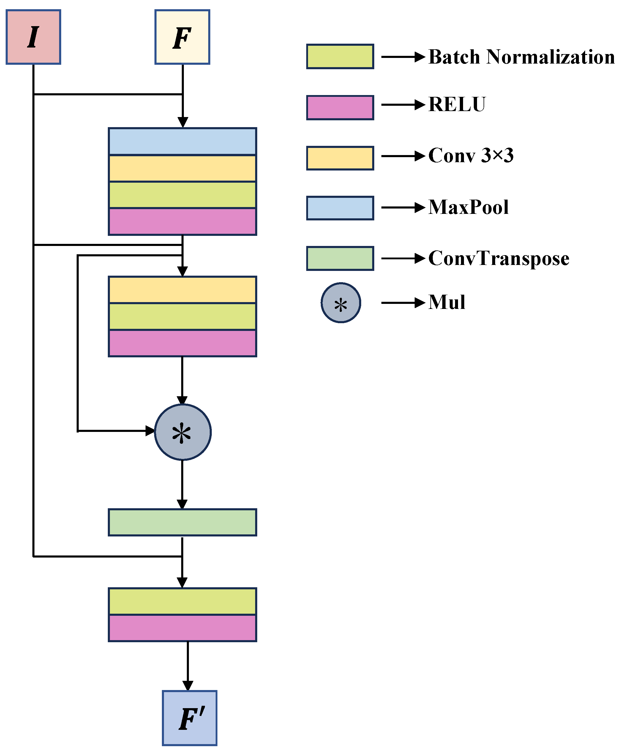
Decoder: The decoder is designed based on a stacked feature segmentation module FSM (Figure 6). Each FSM consists of batch normalization, ReLU activation, 3 × 3 convolution, max pooling, and transposed convolution operations. In particular, the input feature F merges with the skip connection feature I originating from the encoder. Max pooling is applied to reduce redundant information and to enlarge the receptive field, while a 3 × 3 convolution enhances the local feature representation. Then, features are normalized and passed through a nonlinear activation. Finally, features are upsampled to restore the spatial resolution using transposed convolution. During this process, feature I is concatenated with the features processed by the FSM, compensating for the detail loss caused by pooling and enhancing the precision of the segmentation boundaries. Our design can take into account computational efficiency and feature retention capability.

Discriminator: Inspired by the method in [26], we train the discriminator and LCNN using an ADF in the output space to determine whether the segmentation outputs come from the source or target domain. This process aligns the features in normal sea states with those in harsh sea states. In this study, we modify the architecture from [26] to design a new discriminator, which comprises four downsampling blocks and a classification layer; each downsampling block includes a convolutional layer that doubles the number of channels, followed by a downsampling layer. Consequently, the number of channels in the convolutional layers of the downsampling blocks are 64, 128, 256, and 512, respectively.

Each convolutional layer is followed by a batch normalization layer [33] and a LeakyReLU activation function [34]. The LeakyReLU layer aims to address the ‘neuron death’ problem associated with the standard ReLU activation function. When the input is less than zero, LeakyReLU allows these negative values to pass through with a small slope (e.g., 0.01) instead of setting them directly to zero. This design prevents gradient vanishing issues during training, keeping neurons active and facilitating learning of more complex feature mappings. The final classification layer uses convolution to merge the channels and produce the discrimination results.

The training of LCNN and the discriminator alternates between two steps. In the first step, with LCNN’s weights frozen, the discriminator is trained to distinguish segmentation outputs from the source domain (normal sea states) from those of the target domain (harsh sea states) using a binary cross-entropy loss. In the second step, the discriminator’s weights are frozen, and LCNN is updated. LCNN’s total loss function is a combination of its primary segmentation loss ($L_{seg}$) and an adversarial component. To encourage LCNN to generate features that fool the discriminator, the adversarial loss is subtracted from the segmentation loss, weighted by a hyperparameter $\lambda$. The update rule for LCNN is based on $L_{total}=L_{seg}-\lambda L_D$, where we set $\lambda =0.005$. This schedule ensures stable training and effectively aligns the feature distributions across the two domains.

The pseudocode of the used discriminator is shown in Algorithm 1.

Algorithm 1 Discriminator

1: Input: Input tensor $x\in {\mathbb{R}}^{B\times C\times H\times W}$, where B is the batch size, C is the number of channels, $H,W$ are height and width, and n is the number of hidden feature channels.   2: Initialize Layers:   3:        $Block1\leftarrow \mathrm{Conv}2\mathrm{d}(num\_classes,n)$           $\to \mathrm{BatchNorm}2\mathrm{d}\left(n\right)$           $\to \mathrm{LeakyReLU}$           $\to \mathrm{MaxPool}2\mathrm{d}$   4:        $Block2\leftarrow \mathrm{Conv}2\mathrm{d}(n,2\times n)$           $\to \mathrm{BatchNorm}2\mathrm{d}(2\times n)$           $\to \mathrm{LeakyReLU}$           $\to \mathrm{MaxPool}2\mathrm{d}$   5:        $Block3\leftarrow \mathrm{Conv}2\mathrm{d}(2\times n,4\times n)$           $\to \mathrm{BatchNorm}2\mathrm{d}(4\times n)$           $\to \mathrm{LeakyReLU}$           $\to \mathrm{MaxPool}2\mathrm{d}$   6:        $Block4\leftarrow \mathrm{Conv}2\mathrm{d}(4\times n,8\times n)$           $\to \mathrm{BatchNorm}2\mathrm{d}(8\times n)$           $\to \mathrm{LeakyReLU}$   7:        $Classifier\leftarrow \mathrm{Conv}2\mathrm{d}(8\times n,1)$   8: Forward Pass:   9:        $x\leftarrow Block1\left(x\right)$ 10:        $x\leftarrow Block2\left(x\right)$ 11:        $x\leftarrow Block3\left(x\right)$ 12:        $x\leftarrow Block4\left(x\right)$ 13:        $x\leftarrow Classifier\left(x\right)$ 14:        return: x (output tensor)

3. Experiments and Results

3.1. Datasets

Our data source is REDOS [29], which spans two decades, from 1 January 1992 to 31 December 2011. Its model region is 1°N–30°N, 99°E–134°E, covering the entire South China Sea and a part of the Northwestern Pacific Ocean, especially the Luzon strait. REDOS was generated by the South China Sea Ocean Assimilation System, which comprises three components: the Regional Ocean Model System (ROMS), a multiscale three-dimensional (3D) variational data assimilation approach, and a module for quality control of observational data [29,35]. Crucially, the generation of REDOS incorporated atmospheric forcing data such as sea-level pressure and wind fields. This means the dataset inherently contains the complex SSH signatures of typhoon events that occurred during this period. The dataset provides a total of 7306 daily average data points. For training, we use a 10-year dataset (1992–2001) comprising 3653 samples and reserve the one in 2002 with 365 samples for testing. We further generate the eddy detection and ground-truth labels using the Eddy Tracker tool implemented in Python [13,36]. We further label pixels with the class representing the eddy {‘0’: Non-eddy/land/no data, ‘1’: anticyclonic eddy, ‘2’: cyclonic eddy}.

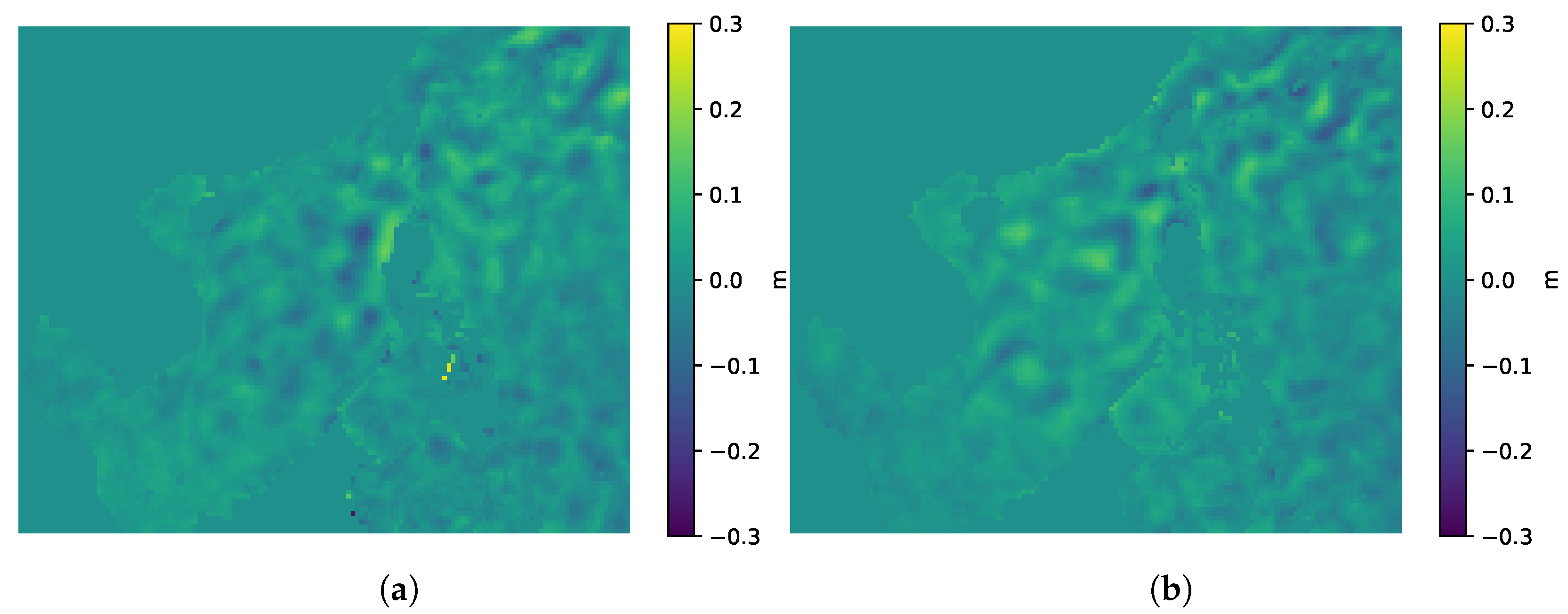
Under harsh sea states, intense meteorological events generally distort the SSH fields. To improve the model’s generalization to harsh sea states, we introduce a data augmentation scheme to create more challenging training scenarios. This scheme employs a 2D GF to simulate heightened SSH perturbations (Equations (1) and (2)). The GF is selected as a pragmatic tool and has properties to effectively model the kind of localized, high-intensity anomalies that typhoons induce on the sea surface, such as central symmetry, controllable amplitude, and rapid attenuation.

As a consequence, the generated perturbation fields are superposed onto the original SSH data. Instead of attempting to replicate the full dynamics of ocean–atmosphere interaction, we aim to enhance the diversity of the input data. By augmenting the baseline REDOS data, which already contains real typhoon signatures, with these controlled perturbations (white noise), we expose the model to a wider range of high-noise conditions. This process serves as a computationally efficient method to improve the model’s robustness, compelling it to learn features that are invariant to such disturbances.

$$\begin{array}{cc}\hfill G_i(x,y)& =A_i·exp(-({\displaystyle \frac{{(x-x_{0i})}^2}{2{\delta }_{xi}^2}}+{\displaystyle \frac{{(y-y_{0i})}^2}{2{\delta }_{yi}^2}})),\hfill \end{array}$$

(1)

$$\begin{array}{cc}\hfill Z_{\mathrm{harsh}}(x,y)& =Z_{\mathrm{original}}(x,y)+\sum _{i=1}^N{G}_i(x,y),\hfill \end{array}$$

(2)

where $Z_{harsh}(x,y)$ denotes the simulated SSH affected by typhoons at position $(x,y)$, $Z_{\mathrm{original}}(x,y)$ denotes the original SSH data at that position, $G_i(x,y)$ represents the i-th two-dimensional Gaussian perturbation, and N is the number of Gaussian perturbations generated for each dataset (randomly between 1 and 3). Amplitude $A_i$ determines the maximum height of the perturbation and is adjustable based on the strength of the simulated typhoon. The center position $(x_{0i},y_{0i})$ specifies the central location of the perturbation, typically corresponding to the typhoon’s center. Standard deviations $({\delta }_{xi},{\delta }_{yi})$ control the spread of the perturbation in the x and y directions, respectively. Smaller values result in more concentrated perturbations, while larger values lead to more dispersed effects. Figure 7 presents a portion of the processed harsh sea states data.

3.2. Parameter Settings and Loss Function

In this model, we set the encoder parameter C to 64, and therefore, the feature map channels increase to 64, 128, and 256 across the three stages, respectively. The Adaptive Spatial–Temporal Scale Perception (ASSP) module in the middle layer reduces the channels to 128, after which three FSMs in the decoder restore the channels to 128, 64, and 32. The dropout in the FEM is given 0.5. The Adam optimizer is used with a learning rate of $1\times {10}^{-3}$ and a batch size of 8. The early-stopping method with a maximum of 150 training epochs is employed.

We employ the most popular Dice loss (Equation (3)) as the loss function, where the Dice coefficient is a set similarity metric commonly used to measure the similarity between two samples. In semantic segmentation tasks, Dice loss is defined as:

$$\begin{array}{cc}\hfill \mathrm{Dice}\mathrm{Loss}& =1-\mathrm{Dice}\mathrm{Coefficient},\hfill \end{array}$$

(3)

$$\begin{array}{cc}\hfill \mathrm{Dice}\mathrm{Coefficient}& ={\displaystyle \frac{2{\sum }_{i=1}^N{p}_i{g}_i+ϵ}{{\sum }_{i=1}^N{p}_i+{\sum }_{i=1}^N{g}_i+ϵ}},\hfill \end{array}$$

(4)

where N is the total number of pixels, $p_i$ is the predicted probability or binary label for pixel i, and $g_i$ is the ground truth binary label for pixel i. Small constant $ϵ$ is added to both the numerator and denominator to prevent division by zero and ensure numerical stability during training.

3.3. Experimental Setup

With the experiments, we evaluate the proposed models’ performance using four metrics: accuracy, precision, Mean Intersection over Union (mIoU), and Dice Coefficient. Accuracy in machine learning represents the overall correctness of the segmentation predictions. It measures the ratio of correctly predicted instances (true positives and true negatives) to the total number of samples, and it is a general metric that considers both positive and negative predictions. Precision focuses on the accuracy of positive segmentation and indicates how reliable the model is when it predicts a sample as positive. It measures the percentage of true positives among all samples labeled as positive by the model. mIoU, a standard metric in semantic segmentation, is determined by averaging the ratio of the overlap to the union between the predicted segments and the ground truth across all classes, providing an overall indication of segmentation quality.

The experiments include the following four parts:

• Model Comparison: It compares different segmentation models for OME detection to validate the effectiveness of the proposed segmentation model. By verifying our model against the existing state-of-the-art models, we aim to demonstrate the proposed model’s improved performance in OME detection.
• Ablation Study: It analyzes the impact of each primary component of the proposed model LCNN. By systematically removing or modifying specific modules, we evaluate the individual contributions of the primary components to the overall performance, quantifying their importance and further validating the rationality of our design choices.
• Adversarial Learning Validation: It focuses on validating the efficacy of the ADF employed in our method. It examines how adversarial training contributes to aligning the feature distributions between normal and harsh sea states. The alignment aims to enhance the segmentation model’s robustness and generalization capability across different sea state conditions.
• Application to actual harsh sea states: We demonstrate the effectiveness of our proposed method applied to actual harsh sea states.

3.3.1. Model Comparison

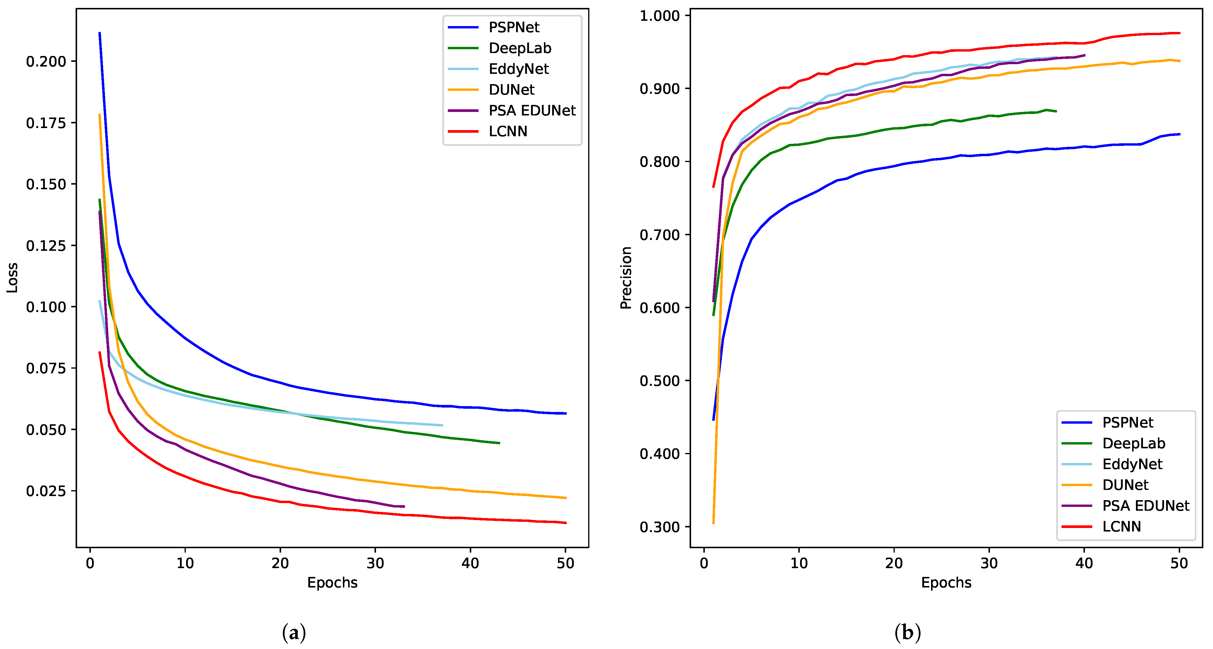
We conduct a comparative analysis between the results of the proposed model (LCNN) and those produced by other existing models, including EddyNet [15] (a UNet-based eddy detection model), PSPNet [18], DeepLabv3 [20], PSA-EDUNet [21], and DUNet [22]. The data used are SLA from the source domain (in normal sea states). Figure 8a illustrates the changes in the loss curves of the models mentioned above during the training. With the increase in training epochs, all models exhibit a steady decline in loss values, while LCNN consistently reaches lower loss levels than the others. Similarly, with the increase in training epochs, the precision of all models progressively improves, while LCNN attains higher precision than the other models (Figure 8b). The final comparative results are presented in

Table 1. Final metrics obtained by different models on the training set. The best results are highlighted in bold.

Method	Accuracy	Precision	mIoU
PSPNet [18]	95.3%	84.2%	77.3%
DeepLab [20]	95.4%	85.9%	76.8%
EddyNet [15]	94.3%	88.3%	69.0%
PSA_EDUNet [21]	96.8%	90.1%	83.1%
DUNet [22]	97.0%	90.0%	84.5%
LCNN	99.3%	97.8%	96.2%

.

Table 2. Final metrics obtained by different models on the test set. The best results are highlighted in bold.

Method	Accuracy	Precision	mIoU
PSPNet [18]	91.1%	70.1%	59.3%
DeepLab [20]	94.1%	80.7%	69.7%
EddyNet [15]	93.8%	86.5%	65.2%
DUNet [22]	95.8%	85.5%	77.1%
PSA_EDUNet [21]	95.9%	86.4%	77.8%
LCNN	97.3%	91.6%	83.4%

provides the average metrics of different models on the SLA data test set. While high accuracy scores are common across all models due to the predominance of background pixels in the data, this metric can be less indicative of the model’s ability to capture fine-grained eddy structures. Metrics more sensitive to segmentation quality, such as Precision and mIoU, reflect the performance differences better.

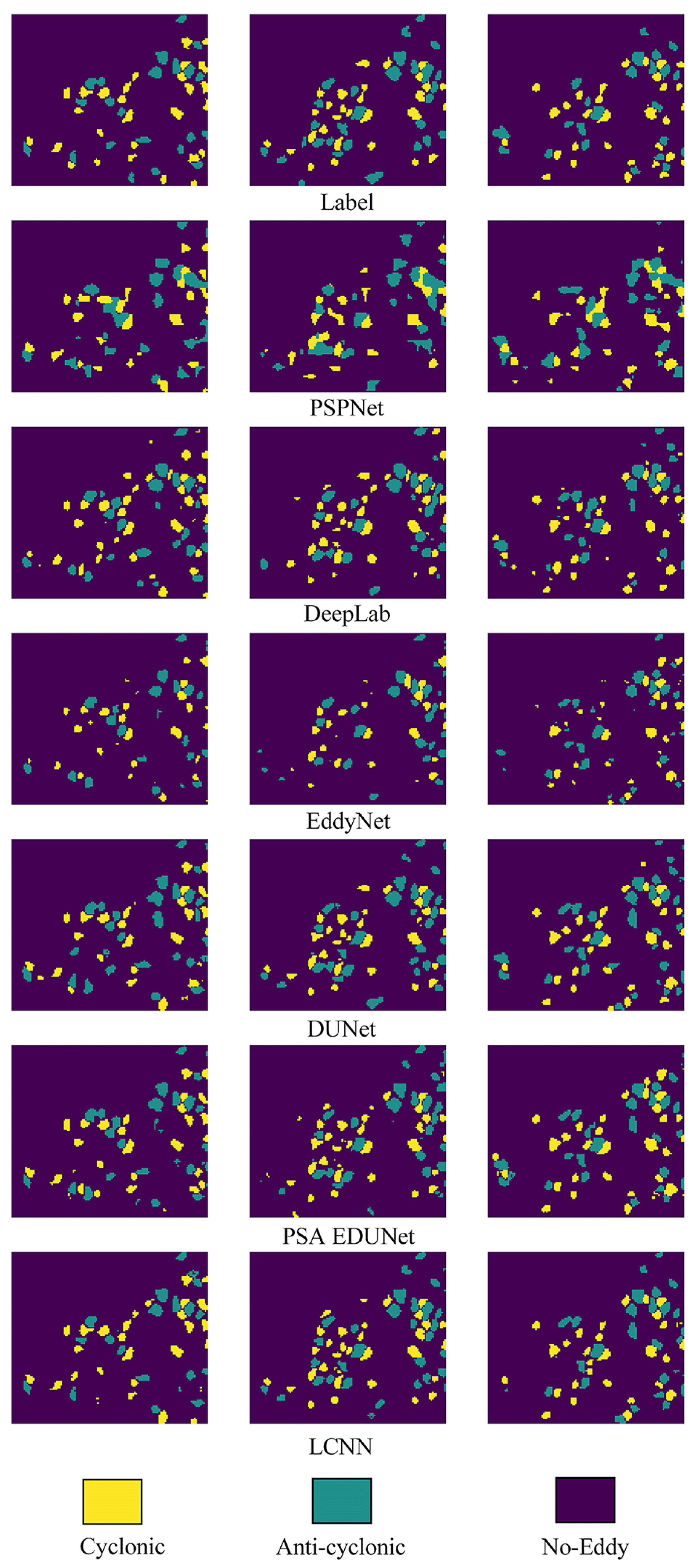
Compared to the superior-performing PSA-EDUNet, LCNN improves accuracy, precision, and mIoU by 1.5%, 6.0%, and 7.2%, respectively. Figure 9 illustrates the segmentation results on representative samples from 1 January 2002 to 3 January 2002. The visually fragmented segmentations produced by PSPNet and Deeplab, for instance, directly correspond to their significantly lower mIoU scores, offering a qualitative insight that complements the average metrics. In contrast, the clear and complete eddy structures segmented by LCNN are consistent with its state-of-the-art performance across all metrics, especially its mIoU of 83.4%.

Table 3. Three types of Dice coefficients obtained by different models on the training set, including background flow, anti-cyclonic eddy, and cyclonic eddy. The best results are highlighted in bold.

Method	No Eddy	Anti-Cyclonic	Cyclonic	Mean
PSPNet [18]	0.021	0.176	0.143	0.050
DeepLab [20]	0.020	0.174	0.141	0.050
EddyNet [15]	0.039	0.203	0.188	0.063
PSA_EDUNet [21]	0.014	0.114	0.101	0.034
DUNet [22]	0.014	0.110	0.088	0.031
LCNN	0.004	0.035	0.027	0.010

shows the average Dice coefficient for various classes on the SLA data training set for different models. Compared to PSPNet, Deeplabv3, EddyNet, PSA-EDUNet, and DUNet, our model (LCNN) achieves an improvement of 81.0%, 80.0%, 89.7%, 71.4%, and 71.4% in the Dice coefficient for anti-cyclonic eddies on the training set; for cyclonic eddies, the improvement was 80.1%, 79.9%, 82.7%, 69.3%, and 68.2%, while for non-eddy regions, the Dice coefficient improved by 81.1%, 80.9%, 85.6%, 73.3%, and 69.3%.

Table 4. Three types of Dice coefficients obtained by different models on the test set, including background flow, anti-cyclonic eddy, and cyclonic eddy. The best results are highlighted in bold.

Method	No Eddy	Anti-Cyclonic	Cyclonic	Mean
PSPNet [18]	0.036	0.338	0.314	0.105
DeepLab [20]	0.026	0.230	0.213	0.071
EddyNet [15]	0.037	0.245	0.234	0.077
PSA_EDUNet [21]	0.018	0.156	0.151	0.049
DUNet [22]	0.017	0.160	0.116	0.043
LCNN	0.014	0.121	0.112	0.037

presents the average Dice coefficients calculated using a weighted average for different classes on the SLA data test set for each model. Compared to PSPNet, Deeplabv3, EddyNet, PSA-EDUNet, and DUNet, LCNN achieves an improvement of 64.3%, 47.3%, 50.6%, 22.4%, and 24.3% in the Dice coefficient for anti-cyclonic eddies on the test set. For cyclonic eddies, the improvement was 64.3%, 47.4%, 52.1%, 25.8%, and 3.4%, while for non-eddy regions, the Dice coefficient improved by 64.8%, 47.9%, 52.0%, 24.4%, and 14.0%.

3.3.2. Ablation Study

Table 5. Results of the ablation experiment. The best results are highlighted in bold.

Method	Accuracy	Precision	mIoU
Baseline	96.3%	89.2%	78.7%
Baseline + SAM	96.8%	90.0%	81.4%
Baseline + CAM	97.0%	90.0%	82.7%
LCNN	97.3%	91.6%	83.4%

shows the design of the ablation study, comparing the model performance across various configurations on the SLA data test set. First, the model with only the Encoder + Decoder (the main framework of the proposed model LCNN) was used as the baseline and achieved good performance. Secondly, the SAM was introduced to the baseline model, resulting in improvements of 0.52%, 0.89%, and 3.46% in accuracy, precision, and mIoU, respectively. Thirdly, we further involved the CAM in the baseline model, and the metrics improved by 0.73%, 0.89%, and 5.08%. It demonstrated that incorporating either SAM or CAM could result in a notable improvement in accuracy. The LCNN model integrated with both SAM and CAM showed improvements of 1.04%, 2.69%, and 5.95% in the metrics compared to the baseline. Notably, the improvement in precision with the joint application of SAM and CAM is particularly significant, indicating a synergistic effect rather than a simple additive combination. These findings provide further evidence of the effectiveness of the proposed attention modules.

3.3.3. Adversarial Learning Validation

In this experiment, the ADF was introduced into several state-of-the-art models, including EddyNet, PSPNet, Deeplabv3, PSA-EDUNet, DUNet, and LCNN.

Table 6. Metrics of different models trained with adversarial learning on the harsh sea states dataset. The best results are highlighted in bold.

Method	Accuracy	Precision	mIoU
PSPNet [18] + ADF	89.0%	63.4%	51.7%
DeepLab [20] + ADF	91.1%	70.4%	58.7%
EddyNet [15] + ADF	85.0%	53.6%	44.3%
PSA_EDUNet [21] + ADF	92.0%	74.5%	58.5%
DUNet [22] + ADF	89.0%	66.4%	57.7%
LCNN + ADF	92.3%	75.7%	62.0%
LCNN	92.0%	78.2%	61.2%

presents the metrics to evaluate the models’ performance on the harsh sea states dataset. Moreover, LCNN without the ADF is included for comparison. Compared to the other models, LCNN with the ADF achieves more satisfactory results. Incorporating the domain discrimination module into the original LCNN would further lead to improvements of 0.33% and 1.31% in accuracy and mIoU, respectively. This selective improvement suggests a strong synergy between the ADF module and the LCNN architecture. We posit that LCNN, with its LKC and attention module, extracts more robust spatial features, providing a superior foundation for the ADF to perform domain discrimination compared to other backbones.

It is important to note that since the labels used in this study are from simulated harsh sea states and not ground truth, the calculated metrics should be viewed as indicative of the relative performance rather than a definitive measure of the approach’s impact. Figure 10 provides the harsh sea states data and the segmentation results of LCNN with or without the ADF, respectively. Compared to LCNN (without the ADF), LCNN + ADF can segment more eddies. The explanation is that harsh sea states present a dual challenge: they not only increase the noise within the data, which can obscure existing features, but also induce the formation of new, less-defined eddies. In the simulated data, this effect was intentionally accentuated to better test the model’s capabilities under challenging conditions and thus demonstrate the validity of our approach.

3.3.4. Application to Actual Harsh Sea States

The International Best Track Archive for Climate Stewardship (IBTrACS) project [37,38] compiles comprehensive historical tropical cyclone best track records from Regional Specialized Meteorological Centers and various other agencies. It provides global tropical cyclone track and intensity data at 3-hour intervals. According to the IBTrACS dataset, we selected 80 instances of SLA data from the period 1991–1994 that were influenced by typhoons in the South China Sea as actual harsh sea states for our experiments. To construct this test set, we employed a spatiotemporal matching process. Specifically, an SLA data sample was selected if two criteria were met simultaneously: (1) at the time of the SLA observation, the center of a tropical cyclone (lat, lon in IBTrACS) was located within the geographical boundaries of our South China Sea study area; and (2) the cyclone’s intensity reached the typhoon category, defined as a maximum sustained wind speed (wmo_wind) of 64 knots or greater.

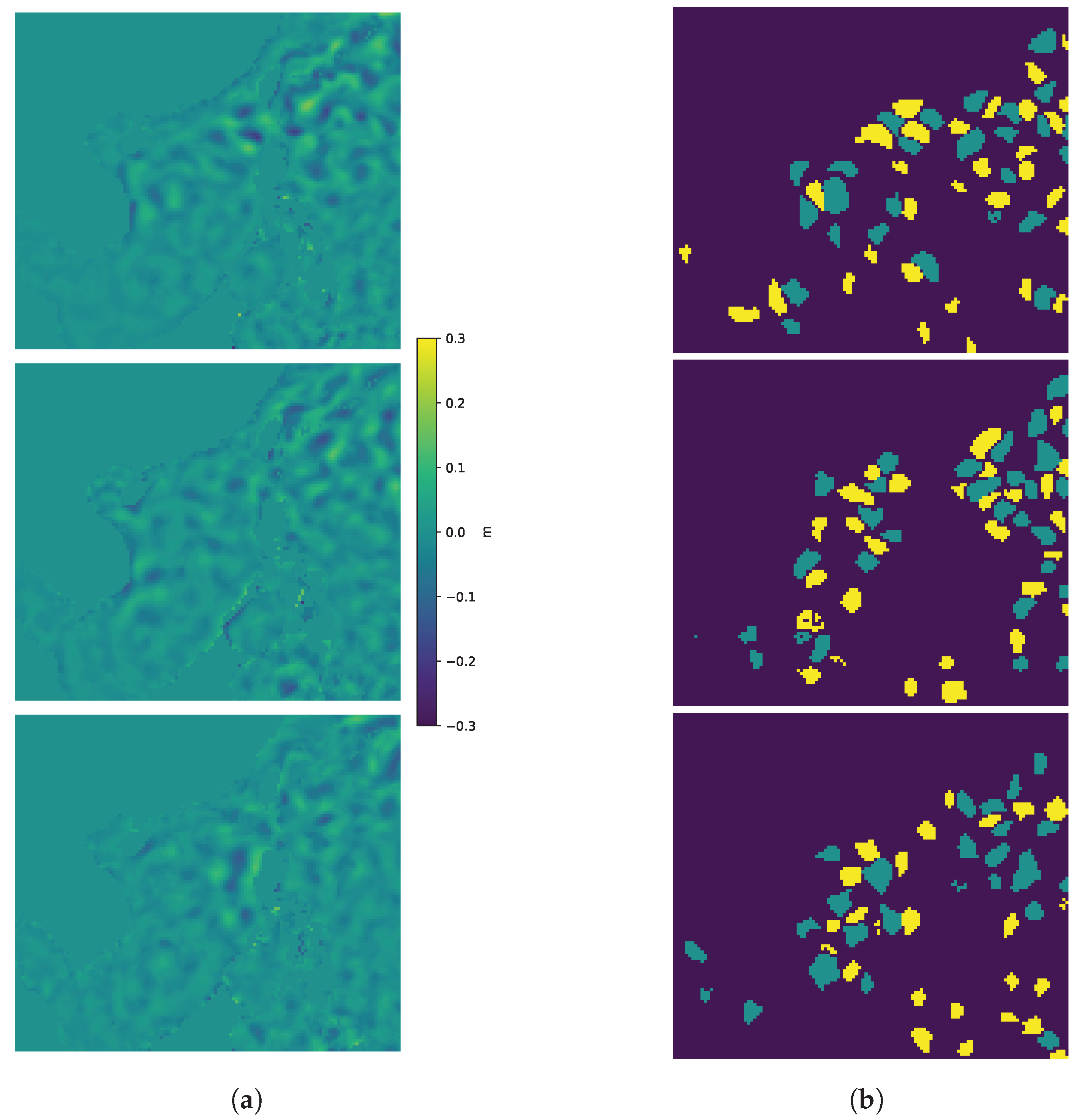
A quantitative comparison of this challenging test set is summarized in

Table 7. Metrics of different models trained with adversarial learning on the actual harsh sea states dataset. The best results are highlighted in bold.

Method	Accuracy	Precision	mIoU
PSA_EDUNet [21]	93.7%	79.8%	65.5%
LCNN	94.5%	87.1%	77.3%
PSA_EDUNet [21] + ADF	93.8%	82.2%	70.1%
LCNN + ADF	95.1%	89.4%	79.9%

. Our proposed LCNN + ADF method maintains a high performance with an mIoU of 79.9%, demonstrating a significant advantage over the baseline models, such as LCNN without ADF (77.3%) and PSA_EDUNet + ADF (70.1%). This performance gap is visually illustrated in Figure 11. Under the disruptive influence of typhoons, our method continues to produce coherent and well-defined eddy segmentations. This case study validates the practical robustness of our proposed method in complex, real-world oceanographic conditions.

4. Discussion

The results of this study strongly indicate that framing the challenge of OME detection under harsh sea states as a domain adaptation problem is a highly effective strategy. The superior performance of the proposed model (LCNN), particularly the 7.2% improvement in mIoU over a strong baseline, is not merely an incremental gain. It highlights the efficacy of its core components in handling the specific challenges of this task. The large kernel convolution expands the model’s receptive field to capture the distorted and irregular shapes of eddies in severe weather more accurately. At the same time, the channel–spatial attention mechanism focuses on the most salient features. Most critically, the success of the adversarial learning framework (ADF) confirms our working hypothesis: explicit learning domain-invariant features are essential to bridge the significant distribution gap between normal and harsh sea states. On the contrary, previous approaches are effective in normal conditions but do not possess a dedicated mechanism to counteract the domain shift induced by extreme weather, which explains their performance degradation.

The primary contribution of this study is to provide a new paradigm for this specific oceanographic challenge. While the other studies have explored multimodal data to enhance eddy detection [39], our research demonstrates that addressing the fundamental problem of domain shift can yield substantial improvements even with single-modal data. The ability to reliably identify OMEs in severe weather has significant scientific and practical implications. It enables a new avenue into critical phenomena, such as typhoon–eddy interactions, and provides a more robust tool for applications requiring high-precision ocean forecasting and maritime safety alerts.

Nevertheless, our study has limitations which also point toward clear directions for future research. Firstly, the model’s reliance on SLA data alone, while powerful, could be a constraint. We plan to develop a multimodal OME detection method that incorporates other oceanic or atmospheric variables, such as SST and flow velocity, to better capture the complex interplay of factors during harsh sea states. Secondly, the use of a 2D Gaussian function to mathematically simulate the impact of harsh sea states is a simplification that lacks underlying physical processes. Although effective, it is a source of uncertainty. To address this, we will seek to integrate coupled atmosphere–ocean models or advanced numerical ocean models in future work. This will provide a more realistic simulation of the nonlinear dynamics of typhoon-induced wind and waves, further closing the gap between synthetic training data and real-world conditions.

5. Conclusions

In conclusion, this study develops a comprehensive solution for the persistent challenge of OME segmentation, particularly under harsh sea states. By reframing the problem through the lens of domain adaptation, we established a new paradigm for this task. A foundational element of our work was the creation of a specialized dataset, which combines real-world normal sea states data with synthetically generated harsh sea state data using a 2D Gaussian function, providing a robust benchmark for model evaluation.

To bridge the domain gap between normal and harsh sea states, we proposed LCNN, a novel end-to-end segmentation model. Its architecture is uniquely designed with LKC and a channel–spatial attention mechanism to enhance spatial feature abstraction and capture irregular eddy forms. Critically, LCNN incorporates an ADF module, which learns domain-invariant features to counteract the data noise and disturbances inherent in harsh sea states. The effectiveness of our approach was validated through extensive experiments, where LCNN consistently outperformed state-of-the-art methods, achieving notable improvements of 1.5%, 6.0%, and 7.2% in accuracy, precision, and mIoU over the strong PSA-EDUNet baseline. This demonstrated performance is more than a technical achievement; it provides a powerful new tool for ocean science. The ability to reliably detect OMEs in severe weather opens new avenues for investigating critical phenomena like typhoon–eddy interactions, significantly improving the precision of localized ocean forecasts, and ultimately contributing to greater maritime safety.

References

1. Black, P.G. Ocean Temperature Changes Induced by Tropical Cyclones; The Pennsylvania State University: University Park, PA, USA, 1983. [Google Scholar]
2. Xing, J.; Wang, F.; Yang, D.; Tan, C.; Ma, X.; Chen, W. Detection and Estimation of Daily Oceanic Mesoscale Eddies From Spaceborne Global Navigation Satellite System-Reflectometry. IEEE Trans. Geosci. Remote Sens. 2025, 63, 5800816. [Google Scholar] [CrossRef]
3. Zhang, Z.; Wang, W.; Qiu, B. Oceanic mass transport by mesoscale eddies. Science 2014, 345, 322–324. [Google Scholar] [CrossRef]
4. Chen, Y.; Tang, D. Eddy-feature phytoplankton bloom induced by a tropical cyclone in the South China Sea. Int. J. Remote Sens. 2012, 33, 7444–7457. [Google Scholar] [CrossRef]
5. Xu, F.; Wen, Z.; Wang, H.; Li, T.; Song, X.; Peng, H. Trends and innovations in ocean mesoscale eddy studies via satellite observation: A bibliometric review. Front. Mar. Sci. 2025, 12, 1577339. [Google Scholar] [CrossRef]
6. Okubo, A. Horizontal dispersion of floatable particles in the vicinity of velocity singularities such as convergences. In Deep Sea Research and Oceanographic Abstracts; Elsevier: Amsterdam, The Netherlands, 1970; Volume 17, pp. 445–454. [Google Scholar]
7. Weiss, J. The dynamics of enstrophy transfer in two-dimensional hydrodynamics. Phys. D Nonlinear Phenom. 1991, 48, 273–294. [Google Scholar] [CrossRef]
8. Sadarjoen, I.A.; Post, F.H. Detection, quantification, and tracking of vortices using streamline geometry. Comput. Graph. 2000, 24, 333–341. [Google Scholar] [CrossRef]
9. Dong, C.; Mavor, T.; Nencioli, F.; Jiang, S.; Uchiyama, Y.; McWilliams, J.C.; Dickey, T.; Ondrusek, M.; Zhang, H.; Clark, D.K. An oceanic cyclonic eddy on the lee side of Lanai Island, Hawai’i. J. Geophys. Res. Ocean. 2009, 114. [Google Scholar] [CrossRef]
10. Nencioli, F.; Dong, C.; Dickey, T.; Washburn, L.; McWilliams, J.C. A vector geometry–based eddy detection algorithm and its application to a high-resolution numerical model product and high-frequency radar surface velocities in the Southern California Bight. J. Atmos. Ocean. Technol. 2010, 27, 564–579. [Google Scholar] [CrossRef]
11. Chelton, D.B.; Schlax, M.G.; Samelson, R.M. Global observations of nonlinear mesoscale eddies. Prog. Oceanogr. 2011, 91, 167–216. [Google Scholar] [CrossRef]
12. Dong, C.; McWilliams, J.; Liu, Y.; Chen, D. Global heat and salt transports by eddy movement. Nat. Commun. 2014, 5, 3294. [Google Scholar] [CrossRef]
13. Pegliasco, C.; Delepoulle, A.; Mason, E.; Morrow, R.; Faugère, Y.; Dibarboure, G. META3.1exp: A new global mesoscale eddy trajectory atlas derived from altimetry. Earth Syst. Sci. Data 2022, 14, 1087–1107. [Google Scholar] [CrossRef]
14. Dong, C.; You, Z.; Dong, J.; Ji, J.; Sun, W.; Xu, G.; Lu, X.; Xie, H.; Teng, F.; Liu, Y.; et al. Oceanic mesoscale eddies. Ocean-Land-Atmos. Res. 2025, 4, 0081. [Google Scholar] [CrossRef]
15. Lguensat, R.; Sun, M.; Fablet, R.; Tandeo, P.; Mason, E.; Chen, G. EddyNet: A deep neural network for pixel-wise classification of oceanic eddies. In Proceedings of the IGARSS 2018—2018 IEEE International Geoscience and Remote Sensing Symposium, Valencia, Spain, 22–27 July 2018; pp. 1764–1767. [Google Scholar]
16. Huang, D.; Du, Y.; He, Q.; Song, W.; Liotta, A. DeepEddy: A simple deep architecture for mesoscale oceanic eddy detection in SAR images. In Proceedings of the 2017 IEEE 14th International Conference on Networking, Sensing and Control (ICNSC), Calabria, Italy, 16–18 May 2017; pp. 673–678. [Google Scholar]
17. Chan, T.H.; Jia, K.; Gao, S.; Lu, J.; Zeng, Z.; Ma, Y. PCANet: A simple deep learning baseline for image classification? IEEE Trans. Image Process. 2015, 24, 5017–5032. [Google Scholar] [CrossRef]
18. Zhao, H.; Shi, J.; Qi, X.; Wang, X.; Jia, J. Pyramid scene parsing network. In Proceedings of the IEEE Conference on Computer Vision and Pattern Recognition, Honolulu, HI, USA, 21–26 July 2017; pp. 2881–2890. [Google Scholar]
19. Duo, Z.; Wang, W.; Wang, H. Oceanic mesoscale eddy detection method based on deep learning. Remote Sens. 2019, 11, 1921. [Google Scholar] [CrossRef]
20. Yurtkulu, S.C.; Şahin, Y.H.; Unal, G. Semantic segmentation with extended DeepLabv3 architecture. In Proceedings of the 2019 27th Signal Processing and Communications Applications Conference (SIU), Sivas, Turkey, 24–26 April 2019; pp. 1–4. [Google Scholar]
21. Zhao, N.; Huang, B.; Yang, J.; Radenkovic, M.; Chen, G. Oceanic eddy identification using pyramid split attention u-net with remote sensing imagery. IEEE Geosci. Remote Sens. Lett. 2023, 20, 1–5. [Google Scholar] [CrossRef]
22. Saida, S.J.; Ari, S. DUNet: Dual U-Net Architecture for Ocean Eddies Detection and Tracking. IEEE Trans. Emerg. Top. Comput. Intell. 2024, 8, 1983–1993. [Google Scholar] [CrossRef]
23. Ding, X.; Zhang, Y.; Ge, Y.; Zhao, S.; Song, L.; Yue, X.; Shan, Y. UniRepLKNet: A Universal Perception Large-Kernel ConvNet for Audio Video Point Cloud Time-Series and Image Recognition. In Proceedings of the IEEE/CVF Conference on Computer Vision and Pattern Recognition, Seattle, WA, USA, 16–22 June 2024; pp. 5513–5524. [Google Scholar]
24. Li, J.; Yu, Z.; Du, Z.; Zhu, L.; Shen, H.T. A comprehensive survey on source-free domain adaptation. IEEE Trans. Pattern Anal. Mach. Intell. 2024, 46, 5743–5762. [Google Scholar] [CrossRef]
25. Zhang, N.; Lu, J.; Li, K.; Fang, Z.; Zhang, G. Source-free unsupervised domain adaptation: Current research and future directions. Neurocomputing 2024, 564, 126921. [Google Scholar] [CrossRef]
26. Wu, X.; Wu, Z.; Guo, H.; Ju, L.; Wang, S. Dannet: A one-stage domain adaptation network for unsupervised nighttime semantic segmentation. In Proceedings of the IEEE/CVF Conference on Computer Vision and Pattern Recognition, Nashville, TN, USA, 20–25 June 2021; pp. 15769–15778. [Google Scholar]
27. Saleh, F.S.; Aliakbarian, M.S.; Salzmann, M.; Petersson, L.; Alvarez, J.M. Effective use of synthetic data for urban scene semantic segmentation. In Proceedings of the European Conference on Computer Vision (ECCV), Munich, Germany, 8–14 September 2018; pp. 84–100. [Google Scholar]
28. Choe, S.A.; Shin, A.H.; Park, K.H.; Choi, J.; Park, G.M. Open-set domain adaptation for semantic segmentation. In Proceedings of the IEEE/CVF Conference on Computer Vision and Pattern Recognition, Seattle, WA, USA, 16–22 June 2024; pp. 23943–23953. [Google Scholar]
29. Zeng, X.; Peng, S.; Li, Z.; Qi, Y.; Chen, R. A reanalysis dataset of the South China Sea. Sci. Data 2014, 1, 1–11. [Google Scholar] [CrossRef]
30. Saida, S.J.; Sahoo, S.P.; Ari, S. Deep convolution neural network based semantic segmentation for ocean eddy detection. Expert Syst. Appl. 2023, 219, 119646. [Google Scholar] [CrossRef]
31. Hu, J.; Shen, L.; Sun, G. Squeeze-and-excitation networks. In Proceedings of the IEEE Conference on Computer Vision and Pattern Recognition, Salt Lake City, UT, USA, 18–23 June 2018; pp. 7132–7141. [Google Scholar]
32. He, K.; Zhang, X.; Ren, S.; Sun, J. Deep residual learning for image recognition. In Proceedings of the IEEE Conference on Computer Vision and Pattern Recognition, Las Vegas, NV, USA, 27–30 June 2016; pp. 770–778. [Google Scholar]
33. Ioffe, S. Batch normalization: Accelerating deep network training by reducing internal covariate shift. arXiv 2015, arXiv:1502.03167. [Google Scholar] [CrossRef]
34. Maas, A.L.; Hannun, A.Y.; Ng, A.Y. Rectifier nonlinearities improve neural network acoustic models. In Proceedings of the International Conference on Machine Learning, Atlanta, GA, USA, 16–21 June 2013; Volume 30, p. 3. [Google Scholar]
35. Peng, S.; Zeng, X.; Li, Z. A three-dimensional variational data assimilation system for the South China Sea: Preliminary results from observing system simulation experiments. Ocean. Dyn. 2016, 66, 737–750. [Google Scholar] [CrossRef]
36. Mason, E.; Pascual, A.; McWilliams, J.C. A New Sea Surface Height—Based Code for Oceanic Mesoscale Eddy Tracking. J. Atmos. Ocean. Technol. 2014, 31, 1181–1188. [Google Scholar] [CrossRef]
37. Knapp, K.R.; Kruk, M.C.; Levinson, D.H.; Diamond, H.J.; Neumann, C.J. The international best track archive for climate stewardship (IBTrACS) unifying tropical cyclone data. Bull. Am. Meteorol. Soc. 2010, 91, 363–376. [Google Scholar] [CrossRef]
38. Gahtan, J.; Knapp, K.R.; Schreck, C.J.; Diamond, H.J.; Kossin, J.P.; Kruk, M.C. International Best Track Archive for Climate Stewardship (IBTrACS), Version v04r00; National Centers for Environmental Information: Asheville, NC, USA, 2022. Available online: https://www.ncei.noaa.gov/products/international-best-track-archive (accessed on 12 September 2024).
39. Zhao, Y.; Fan, Z.; Li, H.; Zhang, R.; Xiang, W.; Wang, S.; Zhong, G. SymmetricNet: End-to-end mesoscale eddy detection with multi-modal data fusion. Front. Mar. Sci. 2023, 10, 1174818. [Google Scholar] [CrossRef]
Figure 1. The main architecture of the domain adaptation-based OME detection method for harsh sea states, where we employ (1) a large kernel convolution to increase the model’s receptive field and deeply extract eddy features and (2) an adversarial learning framework (ADF) to enforce feature alignment between the source (normal sea states) and target (harsh sea states) domains.
Remotesensing 17 03317 g001
Figure 2. Architecture of the proposed attention module.
Remotesensing 17 03317 g002
Figure 3. Architecture of the proposed spatial attention module (SAM), where I denotes the hidden layer size, N denotes the number of heads, and A denotes the number of features allocated to each head.
Remotesensing 17 03317 g003
Figure 4. Architecture of the proposed channel attention module (CAM).
Remotesensing 17 03317 g004
Figure 5. Architecture of the proposed feature extraction module (FEM).
Remotesensing 17 03317 g005
Figure 6. Architecture of the proposed feature segmentation module (FSM).
Remotesensing 17 03317 g006
Figure 7. Representative examples of the synthetic harsh sea states data used as the target domain. (a,b) show two distinct examples from the generated dataset. These images are characterized by synthetically generated complex sea surface patterns and increased background noise, which are designed to challenge the model and enhance its robustness under adverse conditions.
Remotesensing 17 03317 g007
Figure 8. Performance comparison of different models on the source domain training set. The plots illustrate the (a) Dice loss and (b) pixel-level precision for OME segmentation as a function of training epochs. Our proposed model, LCNN, is compared against several baseline models: EddyNet, PSPNet, DeepLabV3, PSA-EDUNet, and DUNet. The curves demonstrate that LCNN consistently achieves a lower loss and a higher precision throughout the training process, indicating superior learning efficiency and convergence performance.
Remotesensing 17 03317 g008
Figure 9. A qualitative comparison of segmentation performance between our proposed model and other methods over a three-day period. The figure is organized in a grid where each column represents a consecutive day from 1 January 2002 (left) to 3 January 2002 (right). Each row displays the results from a different source. This visual evidence highlights that our LCNN model’s outputs most closely align with the ground truth labels across all three days, accurately capturing the dynamic changes in eddy shape and location.
Remotesensing 17 03317 g009
Figure 10. Visual comparison of OMEs’ segmentation performance on simulated harsh sea states data. The figure presents three representative examples, with each row showing a different case of simulated harsh sea state data. For each case, the columns display: (a) The input data, representing a challenging sea state. (b) Segmentation result from our proposed LCNN with the ADF (LCNN + ADF). (c) Segmentation result from the baseline LCNN without the ADF. The key finding is that LCNN + ADF (b) identifies a greater number of eddies with higher fidelity, demonstrating the ADF’s effectiveness in handling data noise and domain shift. In the segmentation maps (b,c), cyclonic eddies are colored yellow, anticyclonic eddies are blue, and the background is purple.
Remotesensing 17 03317 g010
Figure 11. Application of the proposed LCNN + ADF model to real-world harsh sea states. The figure presents three independent examples selected from our real-world dataset to showcase the model’s performance in diverse scenarios. Each row displays a distinct case, consisting of: (a) the observed real-world SLA data, and (b) the corresponding segmentation result generated by our model. This example demonstrates the model’s practical utility in consistently identifying OMEs in a complex, evolving real-world environment, underscoring its potential for operational oceanography. In the segmentation maps (b), cyclonic eddies are colored yellow, anticyclonic eddies are blue, and the background is purple.
Remotesensing 17 03317 g011