Article

Evaluating the Performance of Satellite-Derived Vegetation Indices in Gross Primary Productivity (GPP) Estimation at 30 m and 500 m Spatial Resolution

1
School of Geography and Planning, Chengdu University of Technology, Chengdu 610059, China
2
School of Civil and Hydraulic Engineering, Lanzhou University of Technology, Lanzhou 730050, China
*
Author to whom correspondence should be addressed.
Remote Sens. 2025, 17(19), 3291; https://doi.org/10.3390/rs17193291
Submission received: 10 August 2025 / Revised: 22 September 2025 / Accepted: 24 September 2025 / Published: 25 September 2025

Abstract

Highlights

What are the main findings?
  • Landsat-footprint VIs had strong correlation with tower GPP than MODIS-footprint VIs.
What is the implication of the main finding?
  • NIRv explained tower GPP well both at 30 m and 500 m spatial resolution.

Abstract

Vegetation indices (VIs) have been extensively employed as proxies for gross primary productivity (GPP). However, it is unclear how the spatial resolution effects the performance of VIs in GPP estimation in different biomes when matching the flux tower footprint. Here, we examined the relationship with tower GPP between Landsat-footprint VIs and MODIS-footprint VIs. We first calculated Landsat-footprint VIs (e.g., Normalized Difference Vegetation Index (NDVI), enhanced vegetation index (EVI), two-band EVI (EVI2), near-infrared reflectance of vegetation (NIRv) and kernel Normalized Difference Vegetation Index (kNDVI)) averaged over all the pixels within the footprint and MODIS-footprint VIs with 3 × 3 km or 1 × 1 km around the tower, respectively. We then examined the relationship between Landsat- and MODIS-footprint VIs and tower GPP at monthly scale over 76 FLUXNET sites across ten vegetation types worldwide. The results showed that Landsat-footprint VIs had stronger performance than MODIS-footprint VIs for GPP estimation in all ecosystems, with high improvement on croplands, wetlands, and grasslands and moderate improvements on mixed forest, evergreen needleleaf forest, and deciduous broadleaf forest. Moreover, NIRv showed a stronger correlation with tower-based GPP than NDVI, EVI, EVI2, and kNDVI in ten ecosystems both at 30 m and 500 spatial resolutions. Our findings highlighted the critical role of VIs with high spatial resolution and footprint-aware matching in GPP estimation.

1. Introduction

Gross primary productivity (GPP) represents the total carbon fixed by vegetation through photosynthesis and is a fundamental variable in global carbon cycle studies [1,2,3,4]. As a key indicator of terrestrial ecosystem functioning, GPP directly affects climate–carbon feedback mechanisms, ecosystem health, and biosphere–atmosphere exchanges [5,6,7]. Therefore, accurate estimation of GPP is critical for quantifying terrestrial carbon sinks, evaluating ecosystem resilience under climate variability, and improving earth system models [8].
The eddy covariance (EC) technique has provided direct measurements of ecosystem-scale GPP at flux tower sites in recent decades [9,10,11]. The spatial extent of EC-derived flux measurements within its footprint varied significantly, with longitudinal dimensions spanning from several meters to several kilometers, influenced by sensor height, vegetation characteristics, and surface homogeneity within the measurement area [12]. Therefore, EC measurements cannot be directly integrated to regional or global scales for flux estimation due to their limited spatial representativeness [3].
Satellite remote sensing offers a scalable alternative method by providing continuous, global observations of vegetation activity [7,13]. Vegetation indices (VIs) have become one of the most classic and widely used methods for estimating GPP, as they provide spatially and temporally continuous land surface vegetation information. In particular, spectral VIs derived from multi-band reflectance (e.g., NDVI, EVI, NIRv) serve as robust proxies for canopy greenness, structure, and photosynthetic performance [14,15,16]. These VIs are widely used in empirical models, light use efficiency (LUE) frameworks, and machine learning approaches for regional and global GPP estimation [17,18,19].
VIs such as NDVI [18,20], EVI [15], EVI2 [21,22], NIRv [14,23], and kNDVI [24] have become integral in driving satellite-based GPP products. These VIs are typically combined with site meteorological variables such as PAR and temperature to simulate carbon fluxes [7,11,13,17,25]. However, the performance of these VIs varies depending on spatial resolution, vegetation type, and environmental conditions. Coarse-resolution data (e.g., 500 m from MODIS) are useful for global-scale studies but may miss fine-scale heterogeneity, while higher-resolution data (e.g., 30 m from Landsat or 10 m from Sentinel-2) can better capture local variations but may suffer from lower temporal frequency [26,27]. The spatial resolution of remote sensing data also strongly influences the fidelity of GPP estimation [26]. Coarse-resolution sensors such as MODIS (250–500 m) are widely used due to their global coverage and daily revisit. However, their spatial scale may exceed actual tower footprints by several orders of magnitude, potentially blending land cover types and introducing background noise. Several studies have highlighted the benefits of higher-resolution satellite imagery. Landsat (30 m), Sentinel-2 (10–20 m), and CubeSat constellations (3–5 m) offer opportunities to better capture footprint-level variability [22,26,28]. For example, Sentinel-2-derived red-edge VIs can improve GPP estimation over MODIS VIs at seven cropland towers in North America [22]. A previous study used daily CubeSat NIRvP to track canopy photosynthesis in five intensively managed fields, demonstrating that high spatial and temporal resolutions combined with footprint alignment significantly improved VI–GPP relationships [28].
A crucial but often overlooked issue is the spatial correspondence between satellite pixels and the area actually sampled by EC towers. Unlike fixed plots or field transects, EC towers do not measure a static area. Instead, their effective “footprint”—the dynamic surface area influencing tower measurements—varies with wind direction, canopy height, turbulence, and atmospheric stability [3,12]. This spatial heterogeneity poses a significant challenge: if the VIs extracted from satellite data do not accurately match the EC footprint, the resulting GPP estimation may be biased, especially in mixed or heterogeneous land cover types [28,29]. Previous studies assessed the spatial representativeness of global EC sites using land cover, EVI, and NDVI metrics, finding that fixed buffer zones often diverge substantially from actual footprints [30,31]. Their results revealed that even within a 250 m radius, the difference between a tower’s dynamic footprint and the surrounding fixed-area pixels can lead to “moderate representativeness” or worse. However, many studies use circular buffers (e.g., 1 km or 3 km) to extract satellite data, ignoring this mismatch because actual footprints typically span only 0.01 to 2 km2. This failure to match pixel boundaries introduces unavoidable uncertainties [25,30].
Yet the advantages of finer spatial resolution remain debated. A previous study compared MODIS and Sentinel-2-based EVI2 across eight northern European sites and found that 10 m resolution did not always enhance model accuracy [32]. Moreover, VIs (i.e., NDVI, RDVI, and PRI) from airborne and ground hyperspectral data with footprint-pixel matching in a Mediterranean oak–grassland ecosystem had minimal improvement for GPP estimation on homogeneous surfaces [33].
Therefore, whether VIs with higher resolution can improve GPP estimation depends not only on sensor characteristics but also on ecological context and the degree of spatial heterogeneity. Recent studies reported that Landsat-derived NDVI matching with EC footprints can improve the performance of LUE models by 9~18% in savannas, croplands, and wetlands [34,35,36]. Although a few studies have reported individual VIs under high-resolution imagery, most studies have focused on single ecosystems or regions. It remains unclear how different vegetation indices (e.g., NDVI, EVI, EVI2, NIRv, kNDVI) perform across both coarse and fine spatial resolutions when extracted from flux-matched footprints globally. Moreover, it is unknown whether finer resolution and footprint matching consistently improve GPP estimation across all vegetation types.
In this study, we conducted a global-scale analysis across 76 EC tower sites representing ten major plant functional types. Our objectives are to (1) simulate flux footprints using the flux footprint prediction (FFP) model and extract Landsat-footprint VIs (30 m) and MODIS-footprint VIs (500 m) within matched footprints, and (2) compare the relationships between five commonly used footprint VIs (NDVI, EVI, EVI2, NIRv, kNDVI) and tower-based GPP both at 30 m and 500 m spatial resolution at monthly timescales across different ecosystems.

2. Materials and Methods

2.1. Study Sites

We selected 76 Tier-1 eddy covariance flux sites from the FLUXNET2015 dataset that represent diverse biomes and are globally distributed, primarily across Europe and North America, with additional sites located in Asia and Africa (Figure 1). Based on the widely adopted International Geosphere-Biosphere Programme (IGBP) classification system for global and regional ecosystem studies [37], these sites were categorized into ten vegetation types: cropland (CRO), savannas (SAV), mixed forest (MF), evergreen needleleaf forest (ENF), deciduous broadleaf forest (DBF), evergreen broadleaf forest (EBF), shrubland (SHR), grasslands (GRA), and wetlands (WET). To enable refined carbon flux analysis, cropland sites were further classified into C3 and C4 crops according to crop type in the rotation year. The distinction between C3 and C4 crops lies in their different photosynthetic carbon assimilation pathways and ecological adaptability [38]. C4 crops (e.g., maize) exhibit significant advantages under hot and dry conditions [39], while C3 crops (e.g., wheat, rice) dominate in cooler and temperate climates.
All site data were sourced from the FLUXNET2015 dataset, which provides standardized and quality-controlled eddy covariance observations of carbon, water, and energy fluxes, meteorological variables, and vegetation parameters. This dataset serves as a fundamental resource for studies on the global carbon and water cycles, ecosystem functioning, and climate change [10]. The FLUXNET2015 network integrates flux sites from multiple regional networks and provides continuous, long-term observations with time resolutions ranging from half-hourly to yearly. All data used in this study were obtained from the FLUXNET data portal (https://fluxnet.org/data/fluxnet2015-dataset (accessed on 16 September 2025)).

2.2. Remote Sensing Data and Processing

2.2.1. MODIS Data

MODIS vegetation indices were derived from the MODIS Surface Reflectance 8-day L3 Global 500 m product (MOD09A1 V6.1) from the Terra satellite. The product was downloaded from https://modis.ornl.gov (accessed on 16 September 2025) and included seven spectral bands corrected for atmospheric and aerosol effects [40]. We mainly used three bands, red (620–670 nm), near-infrared (841–876 nm), and blue (459–479 nm), for vegetation index calculations. Based on the availability of valid time series from FLUXNET2015 and MODIS, we selected data from 2000 to 2014 for footprint matching and correlation analysis. All MODIS reflectance data were filtered using the state quality assurance (QA) flags to remove low-quality observations, cloud-contaminated pixels, and outliers, following MODIS Collection 6 data quality guidelines.
Given the coarse resolution of MODIS pixels relative to flux tower footprints, we applied buffer-based extraction strategies depending on vegetation type [25]: for forest sites (EBF, DBF, ENF, MF), a 3 km × 3 km rectangular buffer (12 × 12 pixels) around the tower was used to ensure full coverage of the footprint; for WET, GRA, SAV, SHR, C3, and C4 cropland, a smaller 1 km × 1 km buffer (4 × 4 pixels) was used due to their generally smaller footprints. The buffer sizes of 3 × 3 km and 1 × 1 km were selected to sufficiently cover the footprints of different vegetation types referenced by previous studies [30,35]. The 8-day MODIS-footprint VIs were finally aggregated to 16-day time steps to match the Landsat revisit cycle.

2.2.2. Landsat Data

Landsat surface reflectance products with 30 m spatial resolution were obtained and processed through the Google Earth Engine (GEE) platform. Data sources included Landsat 7 with the Enhanced Thematic Mapper Plus (ETM+) sensor and Landsat 8 with the Operational Land Imager (OLI). All data had undergone atmospheric correction. The red and NIR bands from Landsat 7 (630–690 nm, 770–900 nm) and Landsat 8 (636–673 nm, 851–879 nm) were used to compute vegetation indices such as NDVI and EVI. For each flux site, we extracted a 16-day time series of Landsat VIs within a 3 km buffer centered on the tower. Over 20,000 Landsat VI images were obtained and processed. Cloud-contaminated pixels were removed based on quality assessment bands to ensure accuracy and reliability. We used the parameter-free and flag-free adaptive time-series (PF-free) method to reconstruct the Landsat VIs and MODIS VIs to eliminate the effect of the noise of VI data [41,42].

2.3. Vegetation Indices

Five representative vegetation indices were selected: NDVI, EVI, EVI2, NIRv, and kNDVI. These indices differ in structure, sensitivity, and their relationship with GPP, ranging from traditional ratio-based metrics to enhanced and nonlinear forms. An overview of the five VIs is given in Table 1.

2.4. Footprint Simulation and VI Matching

The FFP model [12] was used to simulate the flux footprint for each site and to spatially match remote sensing vegetation indices with observed GPP. This model, based on eddy covariance theory, estimates source area contributions of surface–atmosphere gas exchanges. Input variables include wind direction (WD), friction velocity (u*), wind speed (V), Obukhov length (L), measurement height (Zm), and canopy height (Hc), and all variables were derived from the half-hourly meteorological records in FLUXNET2015. The FFP model is simple and widely used across vegetation types and long-term datasets, and its open-source code is available at https://footprint.kljun.net (accessed on 16 September 2025).
Footprints were calculated at 30-min intervals and then aggregated into 16-day climatology to align with the Landsat revisit cycle. The 80% cumulative contribution contour was used as the footprint boundary to represent the effective source area [30,47]. The simulation used a 30 m spatial grid for direct alignment with Landsat pixels. For each 16-day period, valid (cloud-free) Landsat pixels within the 80% footprint were averaged to derive Landsat-footprint VIs for each site.

2.5. Statistical Analysis and Evaluation

To assess the ability of vegetation indices to characterize ecosystem GPP across spatial resolutions, the coefficient of determination (R2) was used as the primary statistical metric. The R2 values were used to calculate how well a given VI explains the variance in GPP, and the higher the R2 values, the stronger the correlation of VIs with tower GPP.
All original 16-day VI and tower GPP data were aligned and subsequently aggregated to monthly scale for correlation analysis. Linear regressions were then performed to compute R2 values between each Landsat-footprint-derived VI and MODIS-footprint-derived VI and tower-based GPP.

3. Results

3.1. Evaluation of Footprints and Footprint VIs

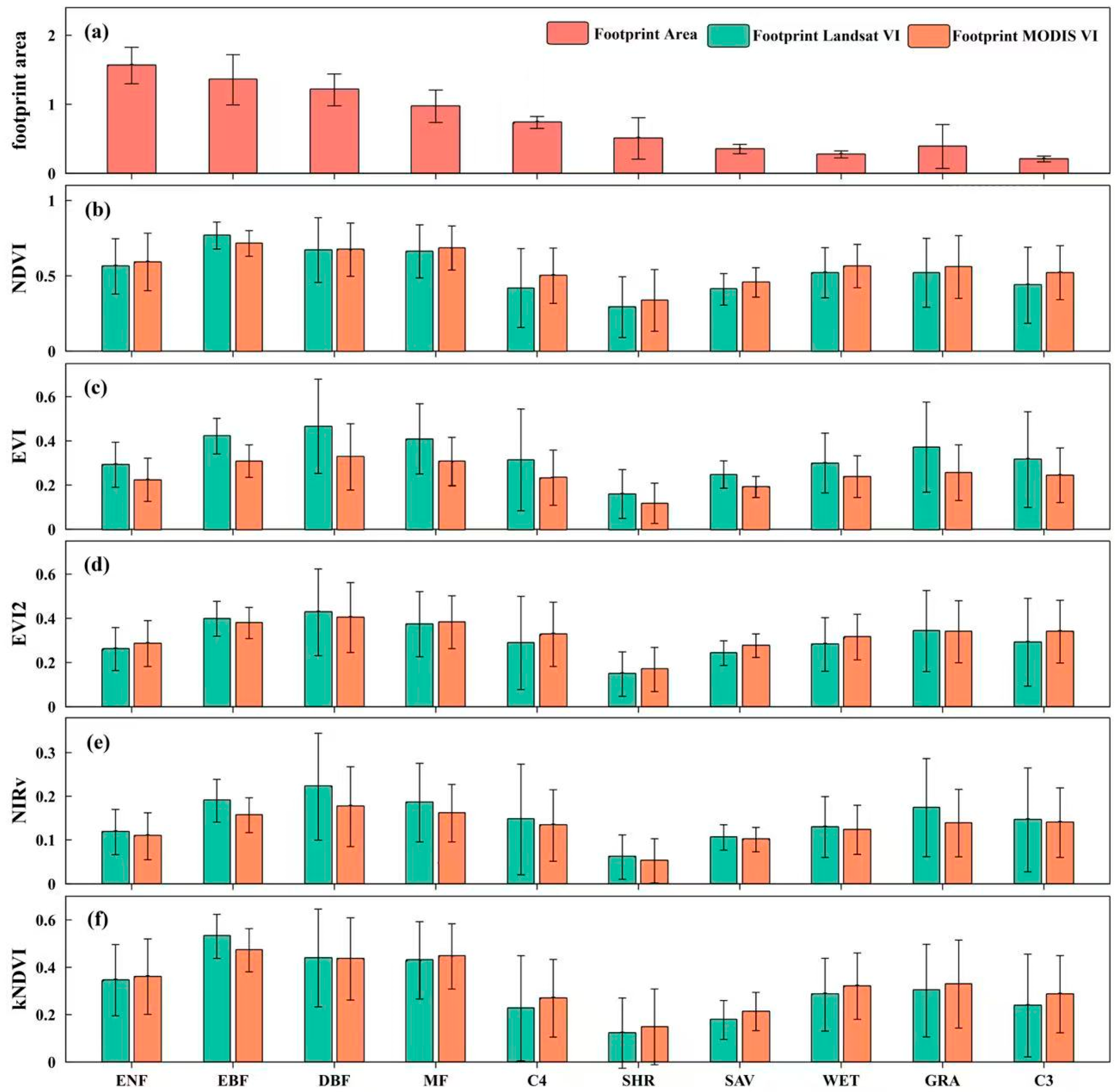
The footprint climatology was calculated at all 76 FLUXNET sites at 16-day intervals, with the 80% contribution contour delineating the extent of each footprint’s climatology. The resulting footprint climatology exhibited a relatively symmetric geometric configuration, while its dimensions and spatial orientation were influenced by wind direction, measurement height, and atmospheric stability. Overall, the spatial range of flux footprint climatology varied from 0.15 km2 to 2.2 km2 at 16-day intervals at a total of 76 sites across ten biomes. Notably, forest ecosystems demonstrated the most extensive footprint areas, ranging from 0.8 km2 to 2.2 km2. In contrast, the footprint areas associated with grassland, wetland, savanna, shrubland, and cropland were comparatively smaller, encompassing approximately 0.15 km2 to 0.9 km2 (Figure 2a).
To further examine the relationship between the footprint area and the heterogeneity of flux footprints both at 30 m and 500 m spatial resolutions, we calculated the Landsat-footprint VIs and MODIS-footprint VIs, respectively. Generally, the MODIS-footprint VIs were extracted by a limited number of pixels, such as 4 × 4 or 12 × 12 pixels for the flux tower footprint, while the Landsat-footprint VIs were extracted by thousands of pixels that correspond to the flux tower footprints. For instance, the largest footprint, approximately 2.2 km2 in evergreen needleleaf forests, is represented by over 2400 pixels for Landsat-footprint VIs, but only 9 pixels for MODIS-footprint VIs.
For cropland, with a radius of less than 500 m, MODIS-footprint VIs are represented only by an individual pixel, while Landsat-footprint VIs encompass at least 230 pixels that entirely overlap the footprints. The difference in pixel numbers between MODIS and Landsat highlights the superiority of remote sensing data characterized by high spatial resolution in representing the flux tower footprint. Furthermore, Landsat-footprint VIs consistently exhibited higher values than MODIS-footprint VIs for forest ecosystems, while the opposite occurred for croplands, wetlands, grasslands, and savannas (Figure 2b–f). Additionally, the discrepancy between Landsat-footprint VIs and MODIS-footprint VIs was notably greater for grasslands, wetlands, savannas, and croplands, whereas it was relatively lower for forest ecosystems.

3.2. Relationships Between VIs and GPP

We analyzed the relationship between MODIS-footprint VIs and Landsat-footprint VIs with observed GPP at both 500 m and 30 m spatial resolutions at the monthly scale. The R2 values were first calculated for each site, and their statistical significance (p-value) was tested. The relationships were statistically significant (p < 0.05) for nearly all sites except EBF. The R2 values were then averaged over the total of 76 sites. In general, MODIS-footprint NDVI, MODIS-footprint EVI, MODIS-footprint EVI2, MODIS-footprint NIRv, and MODIS-footprint kNDVI explained 59%, 72%, 73%, 75%, and 65% of the fluctuation in observed GPP, respectively (Figure 3j). On the contrary, Landsat-footprint NDVI, Landsat-footprint EVI, Landsat-footprint EVI2, Landsat-footprint NIRv, and Landsat-footprint kNDVI exhibited 65%, 74%, 76%, 77%, and 69% of the fluctuation in tower GPP, respectively (Figure 3j). In comparison with MODIS-footprint VIs, Landsat-footprint NDVI improved by 6% in estimating GPP, followed by 4% for Landsat-footprint kNDVI, and 2~3% for Landsat-footprint EVI, Landsat-footprint EVI2, and Landsat-footprint NIRv. This indicated that VIs with high spatial resolution had a greater superiority in estimating GPP than those with coarse spatial resolution. Among all the VIs, on average, the vegetation index of NIRv had the strongest performance in approximating GPP both at 30 m and 500 m spatial resolution (Figure 3a–i).
The R2 values over the 76 sites were then stratified by vegetation types. For each vegetation type, the R2 values, representing the footprint–VI–GPP relationship, were calculated as the mean value over all the sites within the same vegetation type. The R2 values for all ten vegetation types, both at 30 m and 500 m spatial resolution, are illustrated in Figure 3a–i. The potentiality of each MODIS-footprint VI varied by vegetation type in estimating GPP. Overall, DBF (averaged R2 = 0.58~0.75), ENF (averaged R2 = 0.61~0.79), GRA (averaged R2 = 0.63~0.75), and MF (averaged R2 = 0.56~0.83) had the highest correlation with tower GPP, followed by CRO (averaged R2 = 0.56–0.70), SAV (averaged R2 = 0.67~0.69), SHR (averaged R2 = 0.69~0.76), and WET (averaged R2 = 0.54~0.72). EBF had the poorest relationship with GPP (averaged R2 = 0.10~0.37). Meanwhile, Landsat-footprint VIs are similar to MODIS-footprint VIs for GPP estimation with DBF (averaged R2 = 0.74~0.84), ENF (averaged R2 = 0.58~0.78), GRA (averaged R2 = 0.70~0.76), MF (averaged R2 = 0.65~0.84), CRO (averaged R2 = 0.71~0.80), SAV (averaged R2 = 0.65~0.68), SHR (averaged R2 = 0.74~0.80), WET (averaged R2 = 0.62~0.82), and EBF (averaged R2 = 0.10~0.23). Notably, each Landsat-footprint VI improved the performance of GPP estimation by 15% for CRO, followed by 10% for DBF, 8% for WET, 7% for GRA, and 5% for SHR. This demonstrated that the advantage of the high spatial resolution for GPP estimation varied across vegetation types.
To further investigate the manner in which the VI-GPP relationship changed over vegetation types and satellite spatial resolutions, the R2 values were also calculated for all sites within each vegetation type at the monthly scale (Table 2). The degree of improvement in performance of VIs for GPP estimation with the increase in spatial resolution varied across VIs and vegetation types (Table 2). Landsat-footprint VIs had much stronger performance for GPP estimation than did MODIS-footprint VIs for croplands, DBF, MF, and WET ecosystems, and had slightly stronger improvement for SHR and GRA ecosystems. However, Landsat-footprint VIs perform moderately or slightly worse than MODIS-footprint VIs in simulating GPP for ENF ecosystems.
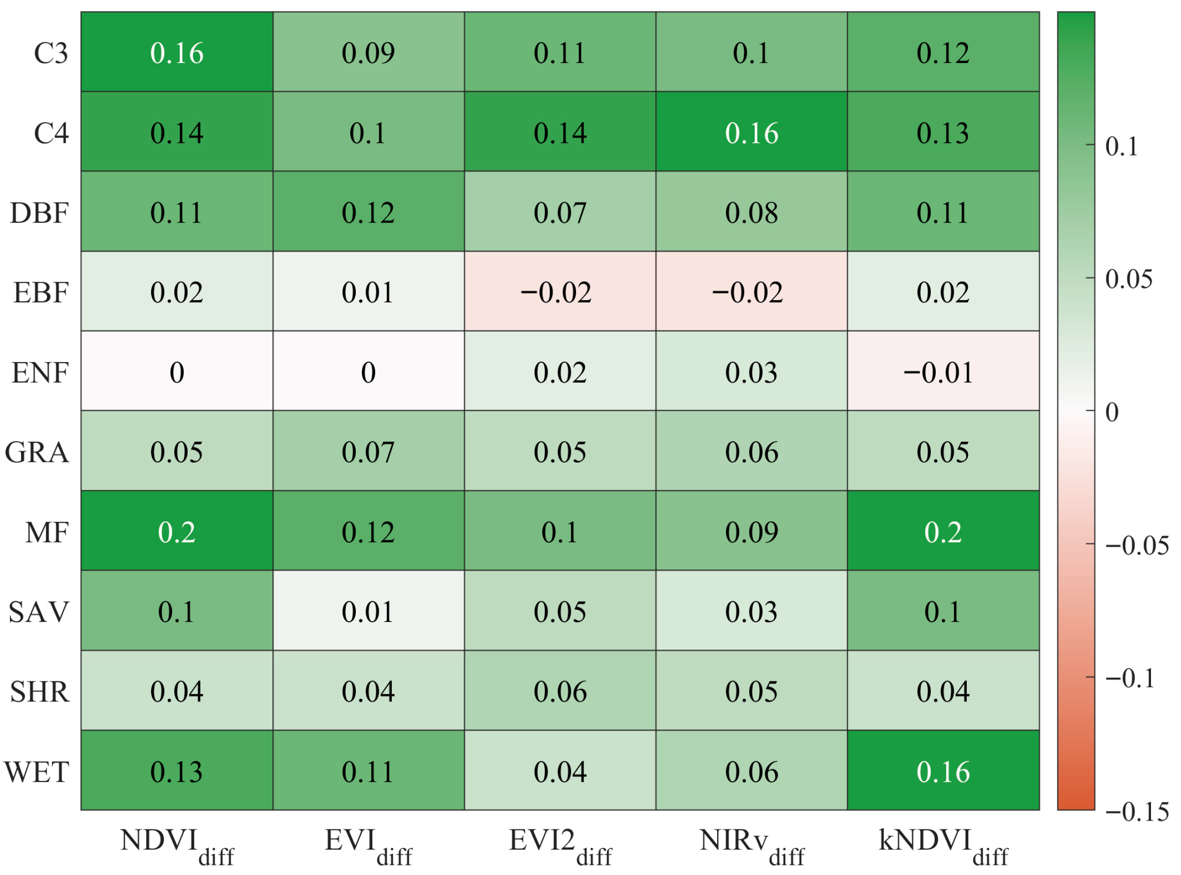
NDVI exhibited significant improvements in performance for GPP estimation at 30 m resolution, with R2 values increased by 16% for croplands, 20% for MF, and 13% for wetlands compared to 500 m resolution, as highlighted in Figure 4. The kNDVI also showed notable improvement, with R2 values increased by 13% for croplands, by 20% for MF, and by 16% for wetlands, and EVI with R2 values increased by 10% for croplands, by 12% for MF, and by 11% for wetlands (Figure 4). However, NIRv had the strongest performance for GPP estimation both at 30 m and 500 m spatial resolution (R2 = 0.63~0.78 at 500 m and R2 = 0.69 ~ 0.86 at 30 m), followed by EVI2 (R2 = 0.63~0.77 at 500 m and R2 = 0.66~0.87 at 30 m) and EVI (R2 = 0.58~0.72 at 500 m and R2 = 0.69~0.85 at 30 m), while NDVI (R2 = 0.40~0.61 at 500 m and R2 = 0.53~0.73 at 30 m) and kNDVI (R2 = 0.42~0.71 at 500 m and R2 = 0.58~0.79 at 30 m) were moderate for GPP estimation (Table 2).
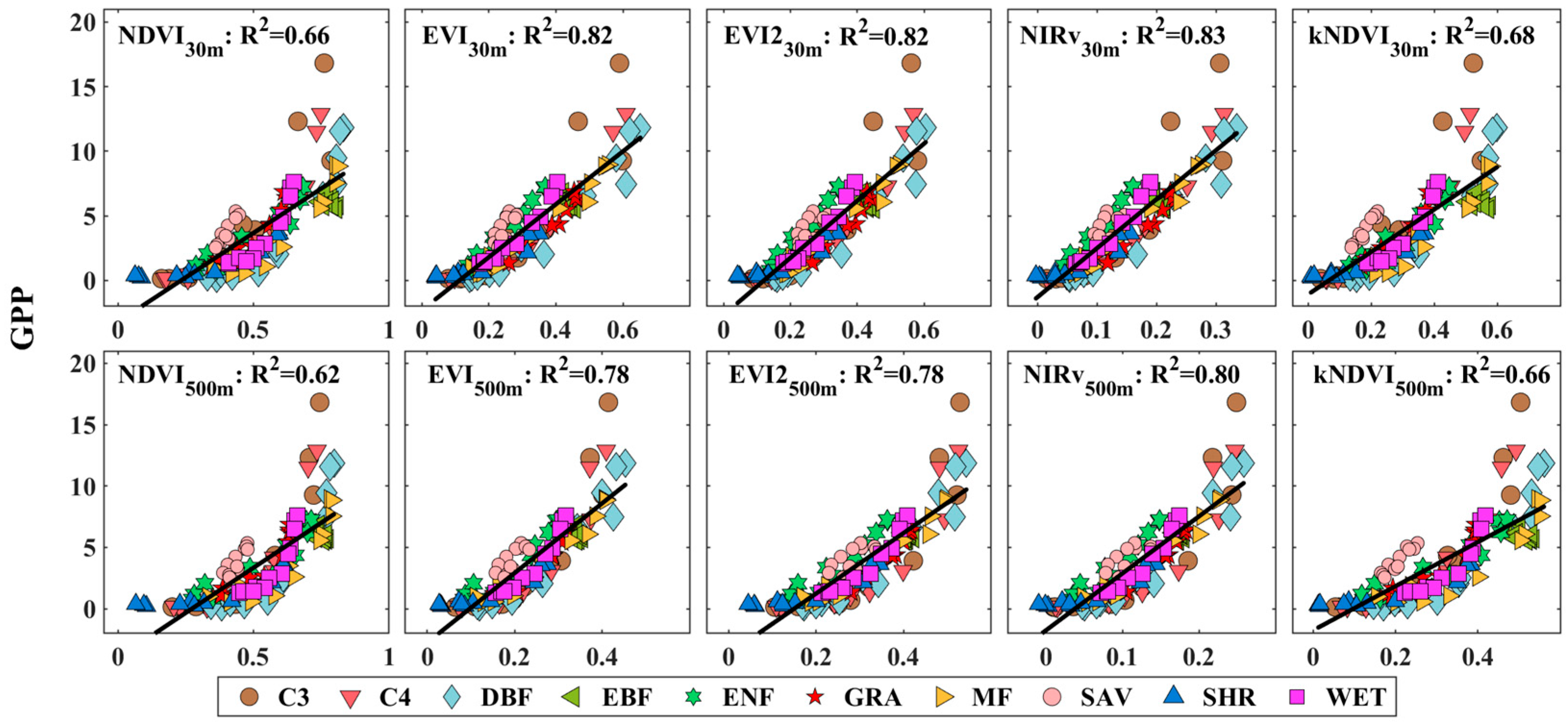
At the vegetation type level, the monthly Landsat-footprint VIs, MODIS-footprint VIs, and tower GPP were first averaged across all years over all sites within each vegetation type, and then the relationships between these VIs and tower GPP at each vegetation type were calculated and are illustrated in Figure 5. EVI, EVI2, and NIRv had a strong relationship with tower GPP across the vegetation types, both at 30 m and 500 spatial resolutions, with R2 ranging from 0.78 to 0.83. On the contrary, NDVI and kNDVI had a much weaker relationship with tower GPP (R2 ranging from 0.62 to 0.68) than did EVI, EVI2, and NIRv. Across vegetation types, NDVI, EVI, EVI2, NIRv, and kNDVI at 30 m spatial resolution were more highly correlated with observed GPP with an improvement in R2 value by 4%, 4%, 4%, 3% and 2%, respectively. Overall, NIRv was the potential proxy for GPP at the biome level, both at 30 m and 500 m spatial resolution.

3.3. Example Cases

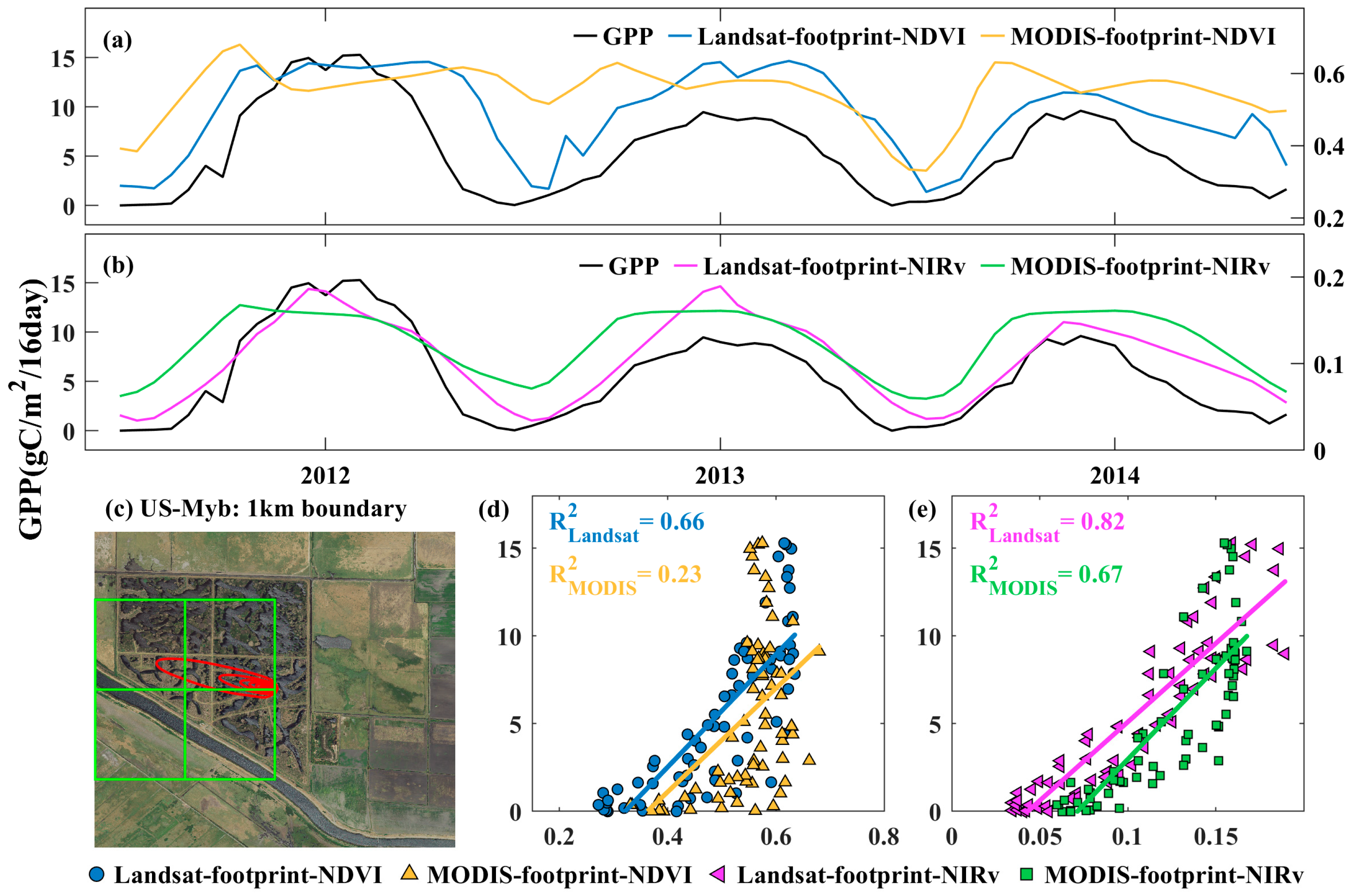
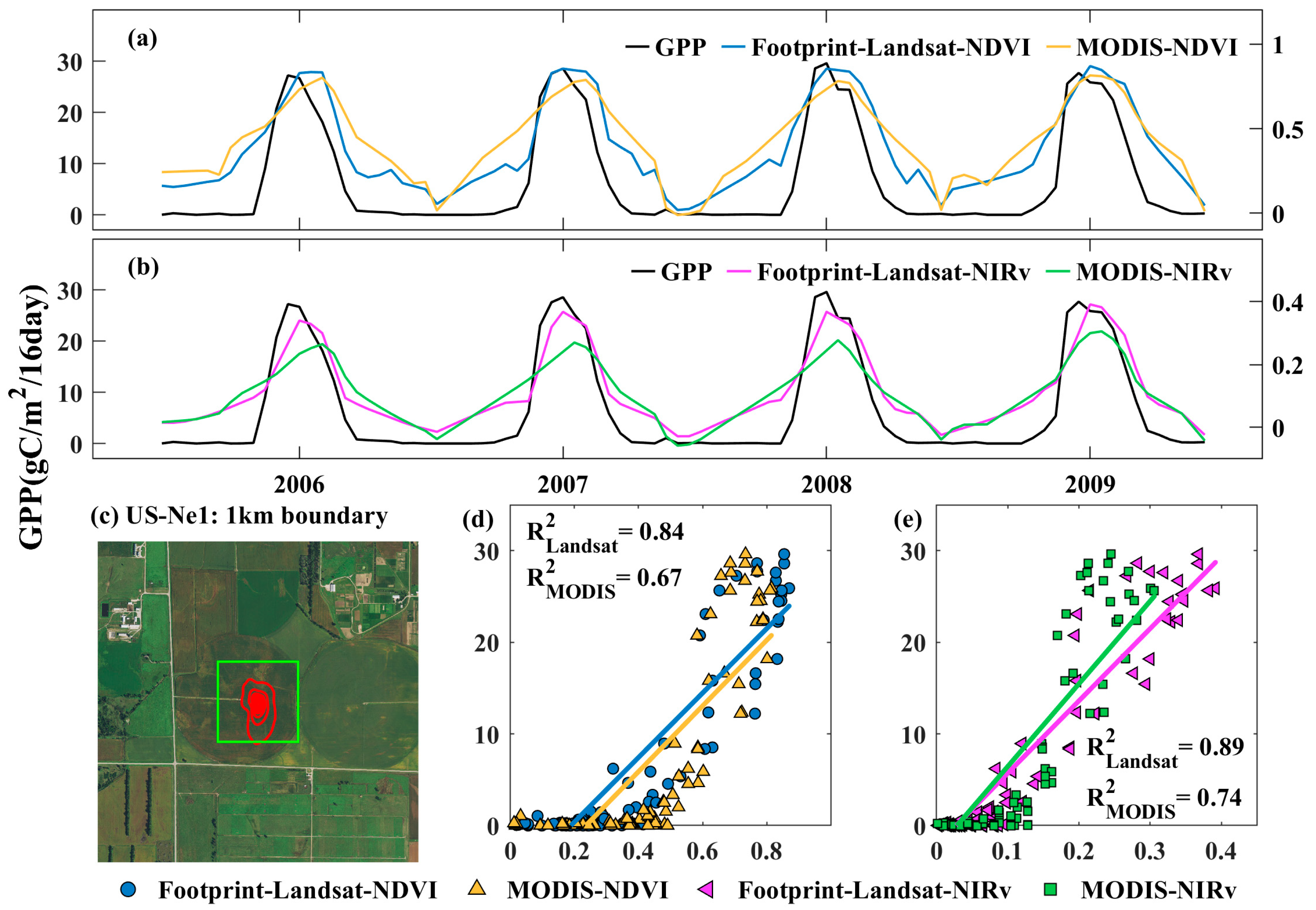
We further selected two heterogeneous sites to evaluate how relationships between VIs and tower GPP changed with satellite spatial resolution. At US-Myb, a highly heterogeneous wetland site in the US, the land is covered with a permanent mixture of water and herbaceous or woody vegetation within 1.5 km around the site (Figure 6c). At US-Ne1, a cropland site in the US, the land is covered with a cropland mixture of maize and soybean within 1.5 km around the site (Figure 7c). We took NDVI and NIRv as an example to examine how footprint VIs varied with 30 m and 500 m spatial resolution. MODIS-footprint NDVI and MODIS-footprint NIRv exhibited a mixture of phenological information when extracting footprint VIs due to the coarse spatial resolution. However, Landsat-footprint NDVI and Landsat-footprint NIRv can better capture the phenology of the site due to their many more pixels within the footprints at 30 m spatial resolution (Figure 6a,b and Figure 7a,b). This further leads to a much higher R2 value of Landsat-footprint VIs and tower GPP than MODIS-footprint VIs (Figure 6d,e and Figure 7d,e).

4. Discussion

In this study, we selected five representative vegetation indices, NDVI, EVI, EVI2, NIRv, and kNDVI, to examine how these VI–GPP correlations varied at 500 m and 30 m spatial resolution.

4.1. The Relationship Between VIs with Matching Footprint and Tower GPP

The spatial resolution of remotely sensed vegetation indices (VIs) is critical for reducing the uncertainty in GPP estimation. Many factors contribute to the uncertainty in GPP modeling. First, finer spatial resolution of remote sensing data can reduce the impact of mixed pixels. Second, finer spatial resolution of remote sensing data can describe a more accurate delineation of the source area represented by EC measurements (i.e., the flux footprint). In this study, our results demonstrated that all five VIs with high spatial resolution significantly enhanced the correlation of tower-derived GPP, especially in heterogeneous ecosystems such as SAV, croplands, and wetlands.
In fact, EC-measured GPP reflects a spatially integrated signal over flux footprints typically ranging from 0.10 to 2.2 km2 [30,35]. When remote sensing data with coarse spatial resolution is substantially coarser than the footprint area, a spatial mismatch between remote sensing data and EC measurement occurs. Previous studies often relied on fixed buffer zones or several MODIS pixels to fully cover tower footprints [11,30,48,49], which can lead to significant scale mismatches, especially in fragmented landscapes, thereby introducing substantial uncertainty into GPP estimation [50].
In our study, we noted that a single MODIS pixel (0.25 km2) often exceeds the actual flux footprint at most FLUXNET sites, whereas Landsat data offer much finer spatial granularity. For example, at the US-Ne1, a maize site, the footprint is as small as a single MODIS pixel (0.1 km2) but more than 200 Landsat pixels (Figure 6 and Figure 7), which enables Landsat data to better capture local spectral heterogeneity and further improve VI-GPP correlation. This is because MODIS-based footprint estimates are generally derived using fixed windows to approximate tower footprints, whereas 30 m Landsat data allow more accurate spatial representation of the flux source area.
Compared to the MODIS data, Landsat imagery with dynamic footprint modeling significantly improved the correlation between Landsat-footprint NDVI and tower-based GPP, particularly in heterogeneous ecosystems. Specifically, the R2 values increased by 15% for cropland (CRO), 13% for wetlands (WET), and up to 20% for mixed forest (MF) (Figure 3; Table 2). These findings are consistent with previous studies [22,28,36], reinforcing the importance of high-resolution remote sensing in mitigating the mixed-pixel problem and improving GPP estimation accuracy under heterogeneous surface conditions. However, in forest ecosystems, our results showed that Landsat data did not consistently outperform MODIS data in predicting GPP. This may be attributed to the relative homogeneity of forest canopies, where medium-resolution MODIS pixels sufficiently capture the canopy-scale signal, and higher-resolution data may even introduce noise from shadow effects.

4.2. The Potential of Each VI in GPP Estimation

All five VIs showed significant correlations with tower-based GPP; however, their performance in GPP estimation varied with VIs. For each VI, NDVI is prone to saturation under dense canopy conditions [15] and is highly sensitive to soil background effects [51], leading to larger errors in highly heterogeneous regions (R2 ranges: 0.40–0.61 for 500 m; 0.53–0.73 for 30 m). Although kNDVI, as a nonlinear generalization of NDVI, partially alleviates saturation through kernel transformation [46], the performance of kNDVI in GPP estimation varied with vegetation types. Overall, NDVI and kNDVI showed the most notable performance in GPP estimation both at 500 m and 30 m spatial resolution.
EVI and EVI2 had similar formulations and thereby exhibited comparable performance in GPP estimation. Compared with NDVI, both EVI and EVI2 had stronger correlation with tower GPP due to their resistance to background noise and saturation [21,44]. Compared with EVI, EVI2 can improve data availability by excluding the blue band [52]. NIRv, combining NDVI and near-infrared reflectance, can better reflect physiological responses of photosynthesis and capture phenological changes more accurately [45,53]. Moreover, NIRv can also reduce background noise and mixed-pixel effects [14,54], and thereby performs most consistently across ten ecosystems, with average R2 values of 0.75 (at 500 m spatial resolution) and 0.77 (at 30 m spatial resolution), which are consistent with previous findings based on MODIS data [45,55].
Different vegetation types exhibited different sensitivity to scale-matching strategies. Landsat-derived NDVI and Landsat-derived NIRv can improve the correlation with tower GPP by 13~20% in heterogeneous ecosystems such as croplands, wetlands, and mixed forests (Figure 3) while they only improve less than 3% in uniform ecosystems such as evergreen needleleaf (ENF) and evergreen broadleaf (EBF) forests (Figure 4). This may be attributed to the larger footprint area and structural uniformity of forest ecosystems, where MODIS pixels already align well with actual flux footprints [56]. In contrast, croplands and wetlands with fragmented landscapes are more affected by mixed-pixel effects, background interference, and phenological asynchrony, where Landsat imagery with high resolution provides clear advantages [29,57]. Our results showed slight improvement of Landsat-derived VIs in GPP estimation at DK-Sor (DBF) and FI-Hyy (ENF), indicating limited gains from remote sensing data with high spatial resolution in structurally homogeneous ecosystems.

4.3. Limitations and Future Perspectives

Although we encompassed a variety of ecosystem types and examined the relationship of Landsat-derived VIs and MODIS-derived VIs with tower GPP at ten vegetation types, some limitations remain. First, we did not explicitly incorporate environmental variables (e.g., temperature, radiation, VPD) when evaluating how spatial resolution affects VI-based GPP estimation. However, previous studies (e.g., [55]) showed that incorporating optimal temperature, radiation, and VPD did not significantly change the observed trends between VIs and GPP. Ref. [28] also demonstrated that high-resolution fusion products exhibited trends consistent with MODIS-derived NIRv and NIRvP, with overall better performance. Additionally, optical remote sensing data are prone to cloud interference. Future studies should integrate multiple data sources (e.g., Sentinel-2, Planet, UAVs) to improve data quality while balancing spatial and temporal resolution.
We revealed that the improvement of spatial resolution significantly enhances footprint matching and GPP estimation in heterogeneous ecosystems such as croplands and wetlands, but with limited effects in forest ecosystems. This suggests that different vegetation types may have distinct optimal spatial resolutions. Ref. [29] found that in tree–grass ecosystems, energy balance models performed best at resolutions below 5 m, with significant error increases above 10 m and relatively stable performance between 30 and 1000 m. Similarly, optimal resolution ranges may exist for GPP estimation. For flat cropland or grassland, Landsat data with 30 m spatial resolution is sufficient to distinguish crop rows, which outperformed MODIS data with 500 m spatial resolution in modeling footprints. Whether further improvements in resolution yield additional benefits remains uncertain. Additionally, in complex terrain areas, the 2D footprint model may not adequately capture slope- or aspect-induced footprint deformation. Combining fine-resolution imagery with digital elevation models (DEMs) and terrain correction is necessary to improve GPP estimation in mountainous ecosystems.
Beyond spatial resolution, the spatial uniformity of surface vegetation at flux tower sites also significantly influences footprint representativeness [33]. Several studies have proposed spatial representativeness metrics, such as albedo variability [58] or heterogeneity indices within a 500 m buffer [59], to quantify surface variability and sampling consistency at global flux tower sites. Other studies (e.g., [30,31]) developed metrics such as the representativeness index to assess the applicability of VI–footprint alignment. These indicators provide a quantitative basis for evaluating the suitability of remote sensing–flux tower integration, but further integration with dynamic footprint modeling is still needed to support accurate and scalable global ecosystem carbon flux monitoring.

5. Conclusions

In this study, we comprehensively evaluated the performance of five vegetation indices (NDVI, EVI, EVI2, NIRv, and kNDVI) in estimating GPP both at 30 m and 500 m spatial resolution at a total of 76 sites encompassing ten worldwide vegetation types at the monthly scale. We achieved pixel-level spatial alignment between remote sensing observations and flux tower measurements through incorporating a dynamic footprint model, thereby substantially reducing uncertainties caused by scale mismatches. Our results indicated that VIs can significantly improve the accuracy in GPP estimation with increases in VIs’ spatial resolution. Compared with MODIS-footprint VIs, Landsat-footprint VIs can improve the explanation of tower GPP by 13~20% in heterogeneous ecosystems such as croplands, wetlands, and mixed forests. In contrast, for structurally homogeneous ecosystems such as evergreen needleleaf and deciduous broadleaf forests, where flux footprints are generally larger, and the MODIS pixels were already sufficient to cover the actual source area. This ensured that MODIS-footprint VIs had comparable performance with Landsat-footprint VIs in GPP estimation in homogeneous ecosystems. Moreover, NIRv exhibited stable performance in GPP estimation both at 500 m spatial resolution (averaged R2 = 0.75) and 30 m spatial resolution (averaged R2 = 0.77). Our findings can help us better understand how the VI–GPP correlation varied with spatial resolution and heterogeneous ecosystems.

Author Contributions

Conceptualization, X.H.; methodology, D.C.; software, D.C.; validation, G.L., Q.X. and L.T.; formal analysis, Y.Y.; investigation, X.H.; resources, X.H.; data curation, D.C.; writing—original draft preparation, D.C.; writing—review and editing, X.H.; visualization, X.H.; supervision, X.H.; project administration, X.H.; funding acquisition, X.H. All authors have read and agreed to the published version of the manuscript.

Funding

This research was funded by the Young Scientists Fund of the National Natural Science Foundation of China (42401426) and the Chengdu University of Technology Everest Team Project (2024ZF11422).

Data Availability Statement

The original contributions presented in this study are included in the article. Further inquiries can be directed to the corresponding author.

Conflicts of Interest

The authors declare no conflicts of interest.

Abbreviations

The following abbreviations are used in this manuscript:
GPPGross Primary Productivity
NDVINormalized Difference Vegetation Index
EVIEnhanced Vegetation Index
EVI2Two-band Enhanced Vegetation Index
NIRvNear-Infrared Reflectance of Vegetation
kNDVIKernel-based Normalized Difference Vegetation Index

References

  1. Chapin, F.S.; Matson, P.A.; Vitousek, P.M. Principles of Terrestrial Ecosystem Ecology; Springer: New York, NY, USA, 2011; ISBN 978-1-4419-9503-2. [Google Scholar]
  2. Ryu, Y.; Berry, J.A.; Baldocchi, D.D. What Is Global Photosynthesis? History, Uncertainties and Opportunities. Remote Sens. Environ. 2019, 223, 95–114. [Google Scholar] [CrossRef]
  3. Schimel, D.; Schneider, F.D. JPL Carbon and Ecosystem Participants Flux Towers in the Sky: Global Ecology from Space. New Phytol. 2019, 224, 570–584. [Google Scholar] [CrossRef]
  4. Xing, X.; Wu, M.; Zhang, W.; Ju, W.; Tagesson, T.; He, W.; Wang, S.; Wang, J.; Hu, L.; Yuan, S.; et al. Modeling China’s Terrestrial Ecosystem Gross Primary Productivity with BEPS Model: Parameter Sensitivity Analysis and Model Calibration. Agric. For. Meteorol. 2023, 343, 109789. [Google Scholar] [CrossRef]
  5. Bonan, G.B.; Doney, S.C. Climate, Ecosystems, and Planetary Futures: The Challenge to Predict Life in Earth System Models. Science 2018, 359, eaam8328. [Google Scholar] [CrossRef]
  6. Le Quéré, C.; Mayot, N. Climate Change and Biospheric Output. Science 2022, 375, 1091–1092. [Google Scholar] [CrossRef]
  7. Xiao, J.; Chevallier, F.; Gomez, C.; Guanter, L.; Hicke, J.A.; Huete, A.R.; Ichii, K.; Ni, W.; Pang, Y.; Rahman, A.F. Remote Sensing of the Terrestrial Carbon Cycle: A Review of Advances over 50 Years. Remote Sens. Environ. 2019, 233, 111383. [Google Scholar] [CrossRef]
  8. Beer, C.; Reichstein, M.; Tomelleri, E.; Ciais, P.; Jung, M.; Carvalhais, N.; Rödenbeck, C.; Arain, M.A.; Baldocchi, D.; Bonan, G.B.; et al. Terrestrial Gross Carbon Dioxide Uptake: Global Distribution and Covariation with Climate. Science 2010, 329, 834–838. [Google Scholar] [CrossRef]
  9. Baldocchi, D.; Falge, E.; Gu, L.; Olson, R.; Hollinger, D.; Running, S.; Anthoni, P.; Bernhofer, C.; Davis, K.; Evans, R.; et al. FLUXNET: A New Tool to Study the Temporal and Spatial Variability of Ecosystem–Scale Carbon Dioxide, Water Vapor, and Energy Flux Densities. Bull. Amer. Meteor. Soc. 2001, 82, 2415–2434. [Google Scholar] [CrossRef]
  10. Pastorello, G.; Trotta, C.; Canfora, E.; Chu, H.; Christianson, D.; Cheah, Y.-W.; Poindexter, C.; Chen, J.; Elbashandy, A.; Humphrey, M.; et al. The FLUXNET2015 Dataset and the ONEFlux Processing Pipeline for Eddy Covariance Data. Sci. Data 2020, 7, 225. [Google Scholar] [CrossRef] [PubMed]
  11. Zhou, Y.; Wu, X.; Ju, W.; Chen, J.M.; Wang, S.; Wang, H.; Yuan, W.; Andrew Black, T.; Jassal, R.; Ibrom, A.; et al. Global Parameterization and Validation of a Two-leaf Light Use Efficiency Model for Predicting Gross Primary Production across FLUXNET Sites. JGR Biogeosci. 2016, 121, 1045–1072. [Google Scholar] [CrossRef]
  12. Kljun, N.; Calanca, P.; Rotach, M.W.; Schmid, H.P. A Simple Two-Dimensional Parameterisation for Flux Footprint Prediction (FFP). Geosci. Model Dev. 2015, 8, 3695–3713. [Google Scholar] [CrossRef]
  13. Anav, A.; Friedlingstein, P.; Beer, C.; Ciais, P.; Harper, A.; Jones, C.; Murray-Tortarolo, G.; Papale, D.; Parazoo, N.C.; Peylin, P.; et al. Spatiotemporal Patterns of Terrestrial Gross Primary Production: A Review. Rev. Geophys. 2015, 53, 785–818. [Google Scholar] [CrossRef]
  14. Badgley, G.; Field, C.B.; Berry, J.A. Canopy Near-Infrared Reflectance and Terrestrial Photosynthesis. Sci. Adv. 2017, 3, e1602244. [Google Scholar] [CrossRef]
  15. Huete, A.; Didan, K.; Miura, T.; Rodriguez, E.P.; Gao, X.; Ferreira, L.G. Overview of the Radiometric and Biophysical Performance of the MODIS Vegetation Indices. Remote Sens. Environ. 2002, 83, 195–213. [Google Scholar] [CrossRef]
  16. Tucker, C.J. Red and Photographic Infrared Linear Combinations for Monitoring Vegetation. Remote Sens. Environ. 1979, 8, 127–150. [Google Scholar] [CrossRef]
  17. Pei, Y.; Dong, J.; Zhang, Y.; Yuan, W.; Doughty, R.; Yang, J.; Zhou, D.; Zhang, L.; Xiao, X. Evolution of Light Use Efficiency Models: Improvement, Uncertainties, and Implications. Agric. For. Meteorol. 2022, 317, 108905. [Google Scholar] [CrossRef]
  18. Yuan, W.; Liu, S.; Zhou, G.; Zhou, G.; Tieszen, L.L.; Baldocchi, D.; Bernhofer, C.; Gholz, H.; Goldstein, A.H.; Goulden, M.L.; et al. Deriving a Light Use Efficiency Model from Eddy Covariance Flux Data for Predicting Daily Gross Primary Production across Biomes. Agric. For. Meteorol. 2007, 143, 189–207. [Google Scholar] [CrossRef]
  19. Zhao, W.; Zhu, Z. Exploring the Best-Matching Plant Traits and Environmental Factors for Vegetation Indices in Estimates of Global Gross Primary Productivity. Remote Sens. 2022, 14, 6316. [Google Scholar] [CrossRef]
  20. Birky, A.K. NDVI and a Simple Model of Deciduous Forest Seasonal Dynamics. Ecol. Model. 2001, 143, 43–58. [Google Scholar] [CrossRef]
  21. Jiang, Z.; Huete, A.R.; Didan, K.; Miura, T. Development of a Two-Band Enhanced Vegetation Index without a Blue Band. Remote Sens. Environ. 2008, 112, 3833–3845. [Google Scholar]
  22. Shirkey, G.; John, R.; Chen, J.; Dahlin, K.; Abraha, M.; Sciusco, P.; Lei, C.; Reed, D.E. Fine Resolution Remote Sensing Spectra Improves Estimates of Gross Primary Production of Croplands. Agric. For. Meteorol. 2022, 326, 109175. [Google Scholar] [CrossRef]
  23. Baldocchi, D.D.; Ryu, Y.; Dechant, B.; Eichelmann, E.; Hemes, K.; Ma, S.; Sanchez, C.R.; Shortt, R.; Szutu, D.; Valach, A.; et al. Outgoing Near-infrared Radiation from Vegetation Scales with Canopy Photosynthesis across a Spectrum of Function, Structure, Physiological Capacity, and Weather. J. Geophys. Res. Biogeoscie. 2020, 125, e2019JG005534. [Google Scholar] [CrossRef]
  24. Camps-Valls, G.; Campos-Taberner, M.; Moreno-Martínez, Á.; Walther, S.; Duveiller, G.; Cescatti, A.; Mahecha, M.D.; Muñoz-Marí, J.; García-Haro, F.J.; Guanter, L.; et al. A Unified Vegetation Index for Quantifying the Terrestrial Biosphere. Sci. Adv. 2021, 7, eabc7447. [Google Scholar] [CrossRef]
  25. Xu, H.; Zhang, Z.; Wu, X.; Wan, J. Light Use Efficiency Models Incorporating Diffuse Radiation Impacts for Simulating Terrestrial Ecosystem Gross Primary Productivity: A Global Comparison. Agric. For. Meteorol. 2023, 332, 109376. [Google Scholar] [CrossRef]
  26. Celis, J.; Xiao, X.; Wagle, P.; Basara, J.; McCarthy, H.; Souza, L. A Comparison of Moderate and High Spatial Resolution Satellite Data for Modeling Gross Primary Production and Transpiration of Native Prairie, Alfalfa, and Winter Wheat. Agric. For. Meteorol. 2024, 344, 109797. [Google Scholar] [CrossRef]
  27. Gelybó, G.; Barcza, Z.; Kern, A.; Kljun, N. Effect of Spatial Heterogeneity on the Validation of Remote Sensing Based GPP Estimations. Agric. For. Meteorol. 2013, 174–175, 43–53. [Google Scholar] [CrossRef]
  28. Kong, J.; Ryu, Y.; Liu, J.; Dechant, B.; Rey-Sanchez, C.; Shortt, R.; Szutu, D.; Verfaillie, J.; Houborg, R.; Baldocchi, D.D. Matching High Resolution Satellite Data and Flux Tower Footprints Improves Their Agreement in Photosynthesis Estimates. Agric. For. Meteorol. 2022, 316, 108878. [Google Scholar] [CrossRef]
  29. Burchard-Levine, V.; Nieto, H.; Riaño, D.; Migliavacca, M.; El-Madany, T.S.; Guzinski, R.; Carrara, A.; Martín, M.P. The Effect of Pixel Heterogeneity for Remote Sensing Based Retrievals of Evapotranspiration in a Semi-Arid Tree-Grass Ecosystem. Remote Sens. Environ. 2021, 260, 112440. [Google Scholar] [CrossRef]
  30. Chu, H.; Luo, X.; Ouyang, Z.; Chan, W.S.; Dengel, S.; Biraud, S.C.; Torn, M.S.; Metzger, S.; Kumar, J.; Arain, M.A.; et al. Representativeness of Eddy-Covariance Flux Footprints for Areas Surrounding AmeriFlux Sites. Agric. For. Meteorol. 2021, 301–302, 108350. [Google Scholar] [CrossRef]
  31. Fang, J.; Fang, J.; Chen, B.; Zhang, H.; Dilawar, A.; Guo, M.; Liu, S. Assessing Spatial Representativeness of Global Flux Tower Eddy-Covariance Measurements Using Data from FLUXNET2015. Sci. Data 2024, 11, 569. [Google Scholar] [CrossRef] [PubMed]
  32. Cai, Z.; Junttila, S.; Holst, J.; Jin, H.; Ardö, J.; Ibrom, A.; Peichl, M.; Mölder, M.; Jönsson, P.; Rinne, J.; et al. Modelling Daily Gross Primary Productivity with Sentinel-2 Data in the Nordic Region–Comparison with Data from MODIS. Remote Sens. 2021, 13, 469. [Google Scholar] [CrossRef]
  33. Pacheco-Labrador, J.; El-Madany, T.S.; Martín, M.P.; Migliavacca, M.; Rossini, M.; Carrara, A.; Zarco-Tejada, P.J. Spatio-Temporal Relationships between Optical Information and Carbon Fluxes in a Mediterranean Tree-Grass Ecosystem. Remote Sens. 2017, 9, 608. [Google Scholar] [CrossRef]
  34. Fu, Y.; Chen, X.; Song, C.; Huang, X.; Dong, J.; Peng, Q.; Yuan, W. High-Resolution Mapping of Global Winter-Triticeae Crops Using a Sample-Free Identification Method. Earth Syst. Sci. Data 2025, 17, 95–115. [Google Scholar] [CrossRef]
  35. Huang, X.; Lin, S.; Li, X.; Ma, M.; Wu, C.; Yuan, W. How Well Can Matching High Spatial Resolution Landsat Data with Flux Tower Footprints Improve Estimates of Vegetation Gross Primary Production. Remote Sens. 2022, 14, 6062. [Google Scholar] [CrossRef]
  36. Huang, X.; Zheng, Y.; Zhang, H.; Lin, S.; Liang, S.; Li, X.; Ma, M.; Yuan, W. High Spatial Resolution Vegetation Gross Primary Production Product: Algorithm and Validation. Sci. Remote Sens. 2022, 5, 100049. [Google Scholar] [CrossRef]
  37. Friedl, M.A.; McIver, D.K.; Hodges, J.C.F.; Zhang, X.Y.; Muchoney, D.; Strahler, A.H.; Woodcock, C.E.; Gopal, S.; Schneider, A.; Cooper, A.; et al. Global Land Cover Mapping from MODIS: Algorithms and Early Results. Remote Sens. Environ. 2002, 83, 287–302. [Google Scholar] [CrossRef]
  38. Monson, R.K.; Li, S.; Ainsworth, E.A.; Fan, Y.; Hodge, J.G.; Knapp, A.K.; Leakey, A.D.B.; Lombardozzi, D.; Reed, S.C.; Sage, R.F.; et al. C4 Photosynthesis, Trait Spectra, and the Fast-efficient Phenotype. New Phytol. 2025, 246, 879–893. [Google Scholar] [CrossRef]
  39. Christin, P.; Osborne, C.P. The Evolutionary Ecology of C4 Plants. New Phytol. 2014, 204, 765–781. [Google Scholar] [CrossRef] [PubMed]
  40. Vermote, E. MODIS/Terra Surface Reflectance 8-Day L3 Global 500m SIN Grid V061 [Data Set]. NASA Land Processes Distributed Active Archive Center. 2021. Available online: https://www.earthdata.nasa.gov/data/catalog/lpcloud-mod09a1-061 (accessed on 23 September 2025). [CrossRef]
  41. Sun, Y.; Peng, D.; Guan, X.; Chu, D.; Ma, Y.; Shen, H. Impacts of the Data Quality of Remote Sensing Vegetation Index on Gross Primary Productivity Estimation. GIScience Remote Sens. 2023, 60, 2275421. [Google Scholar] [CrossRef]
  42. Shen, H.; Ran, Y.; Guan, X.; Chu, D.; Li, D. A Parameter and Flag Adaptive Reconstruction Method for Satellite Vegetation Index Time Series. IEEE Trans. Geosci. Remote Sens. 2025, 63, 4410817. [Google Scholar] [CrossRef]
  43. Running, S.W.; Nemani, R.R.; Heinsch, F.A.; Zhao, M.; Reeves, M.; Hashimoto, H. A Continuous Satellite-Derived Measure of Global Terrestrial Primary Production. BioScience 2004, 54, 547–560. [Google Scholar] [CrossRef]
  44. Rocha, A.V.; Shaver, G.R. Advantages of a Two Band EVI Calculated from Solar and Photosynthetically Active Radiation Fluxes. Agric. For. Meteorol. 2009, 149, 1560–1563. [Google Scholar] [CrossRef]
  45. Zhang, J.; Xiao, J.; Tong, X.; Zhang, J.; Meng, P.; Li, J.; Liu, P.; Yu, P. NIRv and SIF Better Estimate Phenology than NDVI and EVI: Effects of Spring and Autumn Phenology on Ecosystem Production of Planted Forests. Agric. For. Meteorol. 2022, 315, 108819. [Google Scholar] [CrossRef]
  46. Wang, Q.; Moreno-Martínez, Á.; Muñoz-Marí, J.; Campos-Taberner, M.; Camps-Valls, G. Estimation of Vegetation Traits with Kernel NDVI. Isprs J. Photogramm. Remote Sens. 2023, 195, 408–417. [Google Scholar] [CrossRef]
  47. Kumari, S.; Kambhammettu, B.V.N.P.; Adams, M.A.; Niyogi, D. Analysis of Flux Footprints in Fragmented, Heterogeneous Croplands. Meteorol Atmos Phys 2024, 136, 9. [Google Scholar] [CrossRef]
  48. Celis, J.; Xiao, X.; White, P.M.; Cabral, O.M.R.; Freitas, H.C. Improved Modeling of Gross Primary Production and Transpiration of Sugarcane Plantations with Time-Series Landsat and Sentinel-2 Images. Remote Sens. 2023, 16, 46. [Google Scholar] [CrossRef]
  49. Tramontana, G.; Jung, M.; Schwalm, C.R.; Ichii, K.; Camps-Valls, G.; Ráduly, B.; Reichstein, M.; Arain, M.A.; Cescatti, A.; Kiely, G.; et al. Predicting Carbon Dioxide and Energy Fluxes across Global FLUXNET Sites Withregression Algorithms. Biogeosciences 2016, 13, 4291–4313. [Google Scholar] [CrossRef]
  50. Wagle, P.; Gowda, P.H.; Xiao, X.; Kc, A. Parameterizing Ecosystem Light Use Efficiency and Water Use Efficiency to Estimate Maize Gross Primary Production and Evapotranspiration Using MODIS EVI. Agric. For. Meteorol. 2016, 222, 87–97. [Google Scholar] [CrossRef]
  51. Sims, D.A.; Gamon, J.A. Relationships between Leaf Pigment Content and Spectral Reflectance across a Wide Range of Species, Leaf Structures and Developmental Stages. Remote Sens. Environ. 2002, 81, 337–354. [Google Scholar] [CrossRef]
  52. Qiu, B.; Yan, X.; Chen, C.; Tang, Z.; Wu, W.; Xu, W.; Zhao, Z.; Yan, C.; Berry, J.; Huang, W.; et al. The Impact of Indicator Selection on Assessment of Global Greening. GIScience Remote Sens. 2021, 58, 372–385. [Google Scholar] [CrossRef]
  53. Hinojo-Hinojo, C.; Goulden, M.L. Plant Traits Help Explain the Tight Relationship between Vegetation Indices and Gross Primary Production. Remote Sens. 2020, 12, 1405. [Google Scholar] [CrossRef]
  54. Li, Z.-L.; Liu, X.; Zhao, E.; Si, M.; Gao, C.; Wu, H.; Ren, H.; Duan, S.-B.; Tang, R.; Tang, B.-H.; et al. Reflections on Developments and Opportunities of Thermal Infrared Remote Sensing. Innov. Geosci. 2024, 2, 100104. [Google Scholar] [CrossRef]
  55. Huang, X.; Xiao, J.; Ma, M. Evaluating the Performance of Satellite-Derived Vegetation Indices for Estimating Gross Primary Productivity Using FLUXNET Observations across the Globe. Remote Sens. 2019, 11, 1823. [Google Scholar] [CrossRef]
  56. Mukhtar, H.; Yang, Y.; Xu, M.; Wu, J.; Abbas, S.; Wei, D.; Zhao, W. Elevation-dependent Vegetation Greening and Its Responses to Climate Changes in the South Slope of the Himalayas. Geophys. Res. Lett. 2025, 52, e2024GL113276. [Google Scholar] [CrossRef]
  57. Heiskanen, J.; Rautiainen, M.; Stenberg, P.; Mõttus, M.; Vesanto, V.-H.; Korhonen, L.; Majasalmi, T. Seasonal Variation in MODIS LAI for a Boreal Forest Area in Finland. Remote Sens. Environ. 2012, 126, 104–115. [Google Scholar] [CrossRef]
  58. Román, M.O.; Schaaf, C.B.; Woodcock, C.E.; Strahler, A.H.; Yang, X.; Braswell, R.H.; Curtis, P.S.; Davis, K.J.; Dragoni, D.; Goulden, M.L. The MODIS (Collection V005) BRDF/Albedo Product: Assessment of Spatial Representativeness over Forested Landscapes. Remote Sens. Environ. 2009, 113, 2476–2498. [Google Scholar] [CrossRef]
  59. Griebel, A.; Metzen, D.; Pendall, E.; Burba, G.; Metzger, S. Generating Spatially Robust Carbon Budgets from Flux Tower Observations. Geophys. Res. Lett. 2020, 47, e2019GL085942. [Google Scholar] [CrossRef]
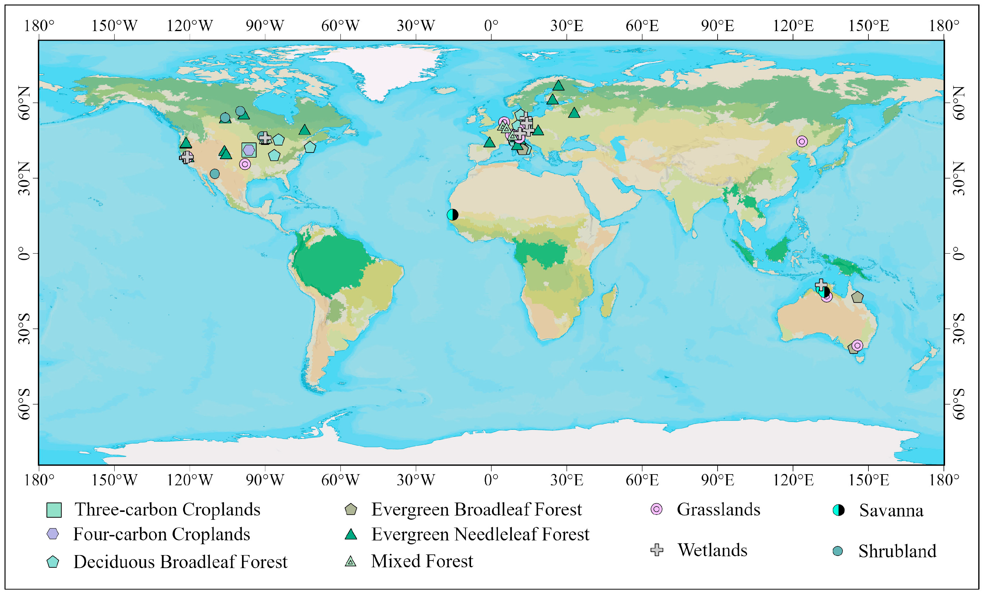
Figure 1. The distribution map of 76 flux sites employed in this study. The base map is a National Geographic-style map provided by ArcGIS Pro 3.1 software.
Remotesensing 17 03291 g001
Figure 2. The grouping error bars are (a) the footprint area distribution of different vegetation types, and (bf) the average values (±standard error) of NDVI, EVI, EVI2, NIRv and kNDVI of Landsat and MODIS data in the flux footprint of each vegetation type. The height of each column represents the average value, and the error column represents the standard error of the average value.
Remotesensing 17 03291 g002
Figure 3. The relationship between MODIS-footprint VIs and Landsat-footprint VIs with tower GPP at the monthly scale across vegetation types (ai) and over the total of 76 FLUXNET sites (j). The height of each bar indicates the mean R2 value for all sites within the corresponding type. Error bars represent the standard error of the mean. The lowercase ‘n’ represents the number of sites.
Remotesensing 17 03291 g003
Figure 4. The differences in explanatory power (ΔR2) for tower GPP between Landsat-footprint VIs and MODIS-footprint VIs across vegetation types. Green shadow indicates better performance of Landsat-derived VIs, with darker green representing stronger improvement in model accuracy.
Remotesensing 17 03291 g004
Figure 5. The relationship of monthly VIs both at 30 m and 500 m spatial resolution with tower GPP for ten vegetation types.
Remotesensing 17 03291 g005
Figure 6. (a): The seasonal cycle of Landsat-footprint NDVI and MODIS-footprint NDVI with tower GPP. (b): The seasonal cycle of Landsat-footprint NIRv and MODIS-footprint NIRv with tower GPP. (c) The footprint boundary of the US-Myb site derived from Landsat and MODIS data. The red irregular ellipse represents the Landsat footprint boundary, and the green rectangle represents the MODIS footprint boundary. (d,e): The scatter plot of the Landsat-footprint NDVI and Landsat-footprint NIRv with tower GPP, respectively.
Remotesensing 17 03291 g006
Figure 7. (a): The seasonal cycle of Landsat-footprint NDVI and MODIS-footprint NDVI with tower GPP. (b): The seasonal cycle of Landsat-footprint NIRv and MODIS-footprint NIRv with tower GPP. (c) The footprint boundary of the US-Ne1 site derived from Landsat and MODIS data. The red irregular ellipse represents the Landsat footprint boundary, and the green rectangle represents the MODIS footprint boundary. (d,e): The scatter plot of the Landsat-footprint NDVI and Landsat-footprint NIRv with tower GPP, respectively.
Remotesensing 17 03291 g007
Table 1. The information of each VI in this study.
VIFull NameFormulaKey CharacteristicsTypical UseReferences
NDVINormalized Difference Vegetation Index N D V I = ρ N I R ρ R e d ρ N I R + ρ R e d Simple, efficient, and widely used.
Sensitive to vegetation greenness and canopy density.
Susceptible to saturation at high LAI and soil background effects.
General vegetation monitoring and long-term productivity modeling.[7,43]
EVIEnhanced Vegetation Index E V I = 2.5 ρ N I R ρ R e d ρ N I R + 6 ρ R e d 7.5 ρ B l u e + 1 Includes blue band and aerosol corrections.
Reduces soil background influence and saturation.
Provides greater sensitivity in high-biomass regions.
Dense forests, cropland, and tropical vegetation.[15,44]
EVI2Two-band Enhanced Vegetation Index E V I 2 = 2.5 ρ N I R ρ R e d ρ N I R + 2.4 ρ R e d + 1 Simplified version of EVI, no blue band required.
Maintains EVI’s advantages in canopy density but increases usability under cloudy or blue-band-absent conditions.
Areas with frequent cloud cover or limited access to the blue band.[21]
NIRvNear-Infrared Reflectance of Vegetation N I R v = N D V I 0.08 × ρ N I R Integrates NDVI and NIR reflectance.
Strongly correlated with GPP and photosynthetic activity.
Less sensitive to background noise and performs well under high LAI.
Modeling GPP, photosynthetic seasonality, and vegetation productivity.[14,45]
kNDVIKernel-based Normalized Difference Vegetation Index k N D V I = t a n h ρ N I R ρ R e d 2 σ 2 t a n h N D V I 2 A nonlinear transformation of NDVI using a tanh kernel.
Reduces saturation effects and enhances GPP correlation.
Designed empirically, not a neural network output.
Complex vegetation structures, high-biomass or heterogeneous ecosystems.[24,46]
Table 2. The R2 values for five VIs and tower GPP at both 30 m and 500 m spatial resolution at the monthly scale across all sites within each of the ten vegetation types.
IGBPNDVIEVIEVI2NIRvkNDVI
30 m500 m30 m500 m30 m500 m30 m500 m30 m500 m
C30.720.560.790.700.770.650.780.670.770.65
C40.730.590.810.710.800.660.830.680.790.67
DBF0.690.580.800.680.770.700.780.700.740.63
EBF0.020.010.020.010.000.020.000.020.020.01
ENF0.590.600.720.720.720.700.740.710.660.67
GRA0.660.610.800.720.770.720.800.740.690.65
MF0.740.540.850.720.870.770.860.780.800.60
SAV0.570.480.710.700.790.740.800.770.680.58
SHR0.660.620.720.680.710.650.690.650.750.71
WET0.530.400.690.580.660.630.690.630.580.42
Disclaimer/Publisher’s Note: The statements, opinions and data contained in all publications are solely those of the individual author(s) and contributor(s) and not of MDPI and/or the editor(s). MDPI and/or the editor(s) disclaim responsibility for any injury to people or property resulting from any ideas, methods, instructions or products referred to in the content.