Revisiting the Terrestrial Water Storage Changes in the Northeastern Tibetan Plateau Using GRACE/GRACE-FO at Different Spatial Scales Considering the Impacts of Large Lakes and Reservoirs

Highlights

What are the main findings?

• The constrained forward modeling (CFM) method is effective for correcting leakage errors in terrestrial water storage (TWS) changes in regions where large lakes and reservoirs co-exist.
• Lake and reservoir water storage and groundwater storage contribute over 85% to TWS changes during 2003–2022.

What is the implication of the main finding?

• Level-2 spherical harmonic coefficients combined with CFM enhance the detection of multi-scale TWS changes and abrupt hydrological events.
• Provides a perspective for water resources monitoring and climate-driven studies in regions where lakes and reservoirs co-exist.

Abstract

The large lakes and reservoirs of the northeastern Tibetan Plateau play a key role in regional water resources, yet their influence on terrestrial water storage (TWS) changes at different spatial scales remains unclear. This study employed the constrained forward modeling (CFM) method to correct leakage errors in level-2 spherical harmonic (SH) coefficients from the Gravity Recovery and Climate Experiment and its follow-on missions (GRACE/GRACE-FO) at three spatial scales: two circular regions covering 90,000 km² and 200,000 km², respectively, and a 220,000 km² region based on the shape of mass concentration (Mascon). TWS changes derived from SH solutions after leakage correction through CFM were compared with level-3 Mascon solutions. Individual water storage components, including lake and reservoir water storage (LRWS), groundwater storage (GWS), and soil moisture storage (SMS), were quantified, and their relationships with precipitation were assessed. From 2003 to 2022, the CFM method effectively mitigated signal leakage, revealing an overall upward trend in TWS at all spatial scales. Signals from Qinghai Lake and Longyangxia Reservoir dominated the long-term trend and amplitude variations of LRWS, respectively. LRWS explained more than 47% of the TWS changes, and together with GWS, accounted for over 85% of the changes. Both CFM-based and Mascon-based TWS changes indicated a consistent upward trend from January 2003 to September 2012, followed by declines from November 2012 to May 2017 and October 2018 to December 2022. During the decline phases, GWS contributions increased, while LRWS contributions and component exchange intensity decreased. LRWS, SMS, and TWS changes were significantly correlated with precipitation, with varying time lags. These findings underscore the value of GRACE/GRACE-FO data for monitoring multiscale TWS dynamics and their climatic drivers in lake- and reservoir-dominated regions.

1. Introduction

The Gravity Recovery and Climate Experiment (GRACE) satellites, launched in March 2002, have enabled the monitoring of the Earth’s time-variable gravity field [1]. Although the original mission ended in June 2017, the GRACE Follow-On (GRACE-FO) mission has continued this record since June 2018 onward [2], providing an unprecedented opportunity to explore terrestrial water storage (TWS) changes over a longer time scale [3]. The GRACE/GRACE-FO datasets facilitate the quantification of regional mass changes resulting from both natural variations and anthropogenic influences on the hydrological cycle [4].

Among the various applications of GRACE/GRACE-FO data, TWS changes derived from satellite gravimetry provide a potential means for better understanding the hydrological dynamics of lakes and reservoirs [5,6]. Previous studies have shown that gravimetric satellites are capable of detecting high-intensity gravity anomaly signals at small scales with concentrated distributions [7]. However, most studies have focused on isolated water bodies, such as the Three Gorges Reservoir, Poyang Lake, or Lake Victoria [8,9,10,11,12], and have largely neglected the interactions among coexisting lakes and reservoirs. The spatially distributed changes in surface water storage alter the local gravity field, and these interactions may introduce additional complexities when analyzing TWS signals over regions containing multiple coexisting water bodies.

The northeastern Tibetan Plateau hosts several representative water bodies, including Qinghai Lake (QHL, the largest lake in China), Longyangxia Reservoir (LYXR, the largest reservoir on the Plateau), and Hala Lake (HLL, located in an endorheic basin). These lakes and reservoirs differ in hydrological characteristics, spatial scales, and watershed types, yet their evolving water dynamics provide distinctive indicators of regional climate change [13]. In recent decades, the hydrological cycle on the Tibetan Plateau has intensified significantly [13]. TWS, as a key component of the hydrological cycle, represents the vertical sum of all water storage component changes, including surface water, groundwater, soil moisture, snow, and canopy water, etc. [14,15,16]. Through the exchange of water and energy at the land surface, TWS plays a crucial role in the climate system [16]. Therefore, quantitatively assessing the contributions of each water storage component to TWS changes and the intensity of their interactions in the northeastern Tibetan Plateau is essential for a comprehensive understanding of how various environmental changes affect regional water resources [17,18].

Prior studies have utilized multi-source remote sensing data to monitor water bodies in the northeastern Tibetan Plateau [19,20], and several works have demonstrated the feasibility of GRACE for tracking mass changes in QHL and LYXR [7,21]. Additionally, Zhan et al. [22] also used GRACE to investigate the impact of surface water bodies such as LYXR, QHL, and HLL on regional TWS changes. However, current studies still lack an assessment of the impacts of signal interference and leakage during forward modeling among coexisting water bodies, as well as a quantitative evaluation of the contributions of individual components to regional-scale TWS changes inversion. To address this gap, this study applies the constrained forward modeling (CFM) method [23,24] to recover TWS signals from GRACE spherical harmonic (SH) solutions at different spatial scales, considering the impacts of large lakes and reservoirs. The CFM method has proven effective in correcting signal leakage errors, avoiding the additional errors that may arise in approaches such as the scaling factor method [25,26,27], which rely on prior information. This method has been applied to the Caspian Sea level changes [28], groundwater depletion in northwestern India [29], and on smaller spatial scales in lake/glacier signals in Scandinavia (~3000 km²) [30], as well as water storage change signals in Lake Volta (~8500 km²) [31], etc.

Building on this, the present study compares the differences in SH and Mascon-based TWS changes and further investigates the responses of TWS and its individual components to climate change. The key scientific questions to be explored are as follows: (1) How large are the impacts of lakes and reservoirs on regional TWS changes, and what are the characteristics of their leakage errors? (2) What are the dominant components driving long-term TWS changes in the northeastern Tibetan Plateau, and how do they vary over time? (3) How are TWS and its components linked to precipitation variability, and what are the temporal characteristics of these relationships?

2. Materials and Methods

2.1. Study Region and Data

2.1.1. Study Area

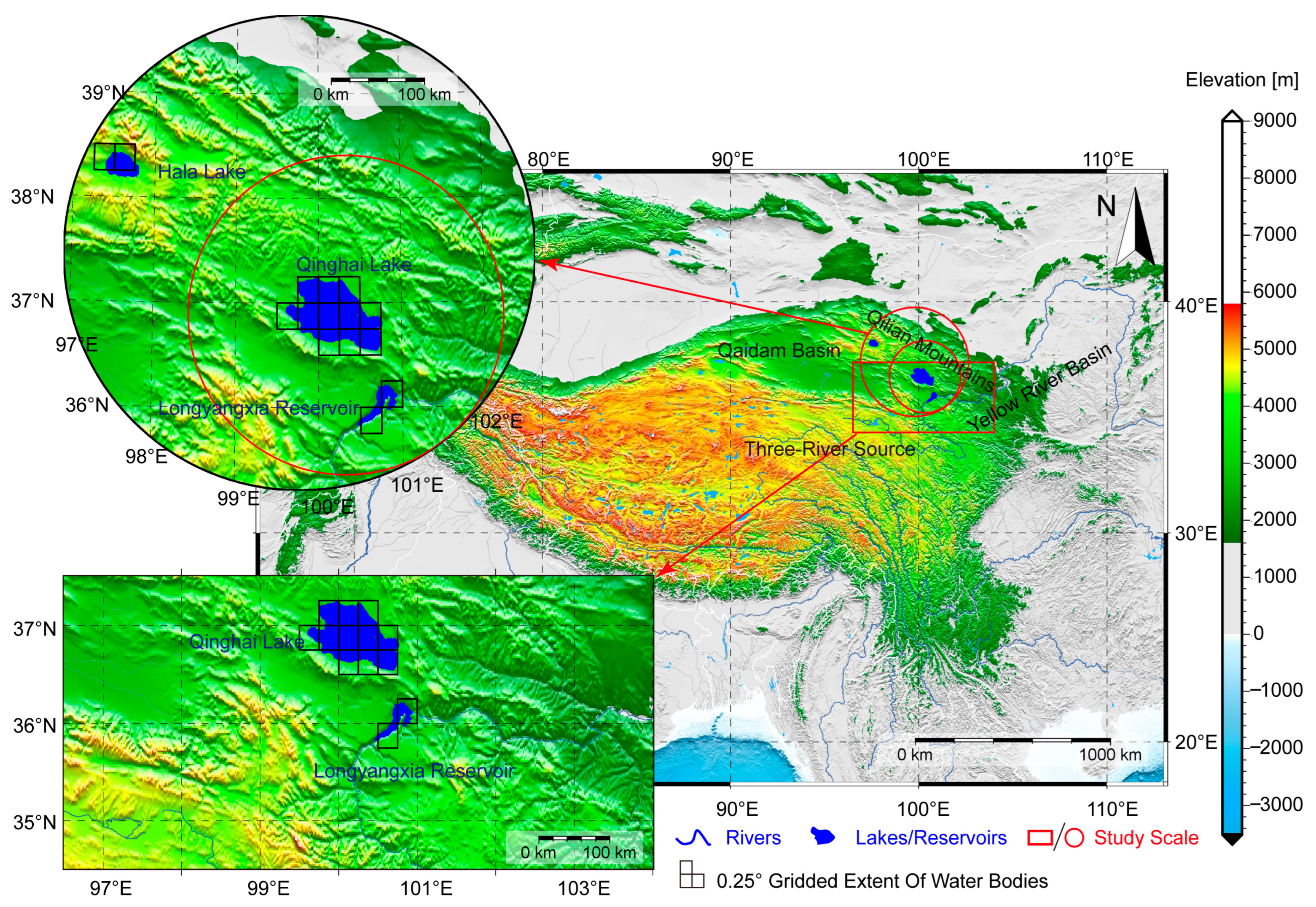
The northeastern Tibetan Plateau is surrounded by the Qaidam Basin, the Qilian Mountains, the Yellow River Basin, and the Three-River Source Basin (see Figure 1). The lakes and reservoirs are situated within the interior of this region. QHL (36°31′–37°15′N, 99°36′–100°46′E) is positioned at the center of the study area with an average elevation of 3194 m, and a surface area of 4533.0 km² as of the end of 2022. The topography of the lake area is characterized by higher elevations in the northwest and lower elevations in the southeast regions. It is bordered by the Datong Mountains to the north, the Riyue Mountains to the east, the Qinghai Nanshan Mountains to the south, and the Xiangpi Mountains to the west, thus forming an enclosed highland lake basin [32]. The HLL (38°11′–38°24′N, 97°24′–97°47′E) is situated to the northwest of QHL and is a closed inland lake on the plateau, with a surface elevation of 4077 m. The LYXR (35°50′–36°12′N, 100°27′–100°55′E), located southeast of QHL, is the only multi-year regulation reservoir in the upper reaches of the Yellow River. It has a normal water level of 2600 m, a storage capacity of 24.7 billion m³, and an inundation area of 383 km², storing water during wet periods and releasing it during dry periods. The study area is located on the margin of the Tibetan Plateau, subject to the Asian summer monsoon and the prevailing westerlies. Consequently, the climate is highly variable, making the regional ecosystem extremely fragile and highly sensitive to climate change.

2.1.2. Study Scales

The GRACE/GRACE-FO satellites are capable of observing terrestrial hydrology; however, the minimum footprint of GRACE/GRACE-FO has varied in previous studies [33]. For instance, Longuevergne et al. [34] and Famiglietti and Rodell [35] demonstrated that GRACE can be effectively applied for large basins over 200,000 km². However, Yi et al. [7] pointed out that the effective resolution of GRACE SH solutions truncated at the 60th degree is about 100,000 km², but smaller areas can be monitored if the regional mass change is highly concentrated. Notably, Vishwakarma et al. [33] reported that the effective resolution of GRACE products is influenced by various processing procedures.

This study focused on various constraint scales differing in spatial extent and shape. As shown in Figure 1, this study applied GRACE/GRACE-FO data at two circular areas of about 90,000 km² and 200,000 km² (referred to as CIRC9 and CIRC20, respectively). Additionally, based on the original spatial resolution of 3° × 3° of the JPL Mascon spherical cap mass concentration blocks, this study selected two rectangular mass blocks that just cover QHL and LYXR, with an approximate area of 220,000 km² (designated as MASC22).

2.1.3. GRACE/GRACE-FO Data

The GRACE/GRACE-FO data include Release-06 monthly gravity field SH coefficient solutions from three institutions: the Center for Space Research, University of Texas at Austin, United States (CSR), the Jet Propulsion Laboratory in Pasadena, California, United States (JPL), and the GeoForschungsZentrum in Potsdam, Germany (GFZ). Additionally, the Release-06 Mascon solutions from CSR, JPL, and the Goddard Space Flight Center in Greenbelt, Maryland, United States (GSFC) are used for comparison. The CSR Mascon solution has a grid resolution of 0.25° × 0.25°, estimated from a 1-degree equal-area mascons [36]. The JPL Mascon solution has a grid resolution of 0.5° × 0.5°, with an original resolution of 3.0° × 3.0°, covering a total of 4551 mass blocks worldwide [37]. This scheme applies the Coastline Resolution Improvement filter [38]. The GSFC Mascon solution has a grid resolution of 0.5° × 0.5°, with an original data resolution of 1-arc-degree equal-area mascons [39].

2.1.4. Lake and Reservoir Water Storage Changes

Surface water bodies such as QHL, HLL, and LYXR within the study area can influence the GRACE data inversion. To obtain their water level and storage changes, satellite altimetry data and in situ observations were utilized. For QHL, monthly average water levels and corresponding water storage changes from 21 June 1995, to the present were obtained from the Hydroweb database, which compiles observations from multiple satellite missions, including Topex/Poseidon, GFO, ERS2, Jason-1/2, Envisat, among others. Missing water level data were filled using cubic spline interpolation. A regression relationship between water level and water storage change was established, enabling the estimation of missing storage data based on the interpolated water levels. For HLL, monthly water level and storage change data from January 2003 to August 2018 were sourced from Li et al. [40], while data from September 2018 to December 2022 were retrieved from the Hydroweb database. Analyses by Li et al. [40] indicate that their dataset is generally consistent with the satellite altimetry data from the Hydroweb database, but may exhibit superior temporal continuity and temporal resolution. Therefore, the satellite altimetry data were corrected based on the Li et al. [40] product to ensure consistency within the dataset. Missing values were estimated following the same method for QHL. Observed water level and storage changes of LYXR from April 2006 to December 2022 were acquired from the Yellow River Conservancy Commission of the Ministry of Water Resources. For the missing reservoir water level data from January 2003 to March 2006, the study utilized the statistical results of Yi et al. [7] and applied a binomial regression model to construct a reservoir capacity curve, thereby predicting the missing reservoir storage for this period.

The total water storage change of each lake or reservoir within the study area was divided by its occupied area within the 0.25° × 0.25° grid to obtain the equivalent water height for each grid cell corresponding to the water body. Subsequently, an area-weighted averaging over the entire study area was applied to derive the regionally averaged equivalent water height, yielding the lake and reservoir water storage (LRWS) time series at CIRC9, CIRC20, and MASC22 spatial scales.

2.1.5. GLDAS Land Surface Models and Precipitation Data

NASA’s Global Land Data Assimilation System (GLDAS) aims to generate optimal land surface states and fluxes by integrating satellite and ground-based observational data with advanced land surface modeling and data assimilation techniques [41]. GLDAS-2 comprises three versions: 2.0, 2.1, and 2.2. The GLDAS-2.2 daily data from the Catchment Land Surface Model, starting on 1 February 2003, used initial conditions from GLDAS-2.0, and included data assimilation from GRACE TWS changes [42]. This study uses GLDAS-2.2 daily data to obtain groundwater storage (GWS), soil moisture storage (SMS), snow water equivalent (SWE), and canopy water storage (CWS) changes. To derive monthly datasets from the daily data, daily values were averaged for each month, generating monthly mean fields for all water storage components. The spatial resolution of the data is 0.25°.

Precipitation data were obtained from the Global Precipitation Climatology Centre (GPCC), established in 1989 at the request of the World Meteorological Organization, and is operated by the German Weather Service under its auspices. The GPCC precipitation products have been widely applied in global hydrometeorological research [31,43,44,45], with Yang et al. [44] demonstrating their relatively superior performance in the inland regions of the Tibetan Plateau. This study used the GPCC Monitoring Product, freely available online (http://gpcc.dwd.de, accessed on 28 June 2025). The GPCC Monitoring Product data were at a 1° grid resolution, and this study applied linear interpolation to resample them to a 0.25° resolution for comparative analysis.

2.2. Method

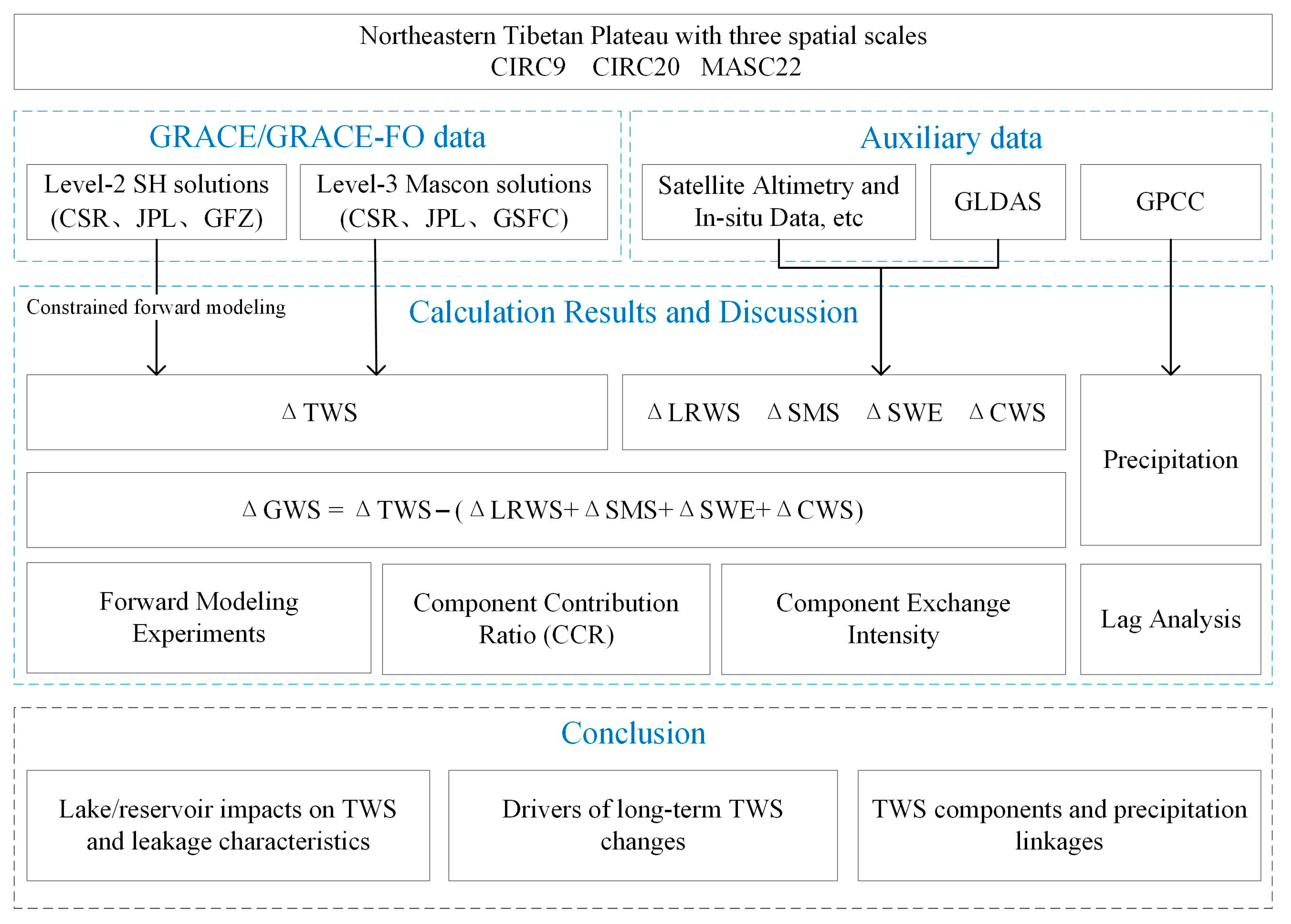
The overall methodological framework and data analysis workflow of this study are illustrated in Figure 2. GRACE/GRACE-FO satellite gravity, satellite altimetry, and the GLDAS hydrological model data were employed to estimate TWS changes and each storage component at three spatial scales, including LRWS, SMS, SWE, CWS, and GWS. Forward modeling experiments, analyses of component contribution ratio (CCR) and component exchange intensity, together with lag-correlation analysis using GPCC precipitation data, were conducted to address the three central scientific questions posed in this study. The following methodology section provides a detailed description of the overall methods.

2.2.1. Satellite Gravity Inversion of TWS Changes

For the GRACE SH solutions, the changes of equivalent water height were calculated from the SH coefficient solutions of each month using the equation provided by Wahr et al. [46]:

$$∆h\left(\theta ,\phi \right)={\displaystyle \frac{a{\rho }_{ave}}{3{\rho }_w}}\sum _{l=0}^N\sum _{m=0}^l{\tilde{P}}_{lm}(cos\theta ){\displaystyle \frac{2l+1}{1+k_l}}\times (∆C_{lm}\cos \left(m\phi \right)+∆{\mathrm{S}}_{lm}\sin \left(m\phi \right))$$

Here, $∆h$ represents the equivalent water height, $\theta$ and $\phi$ are colatitude and longitude of the observation point, $a$ is the Earth’s mean radius, ${\rho }_{ave}$ is the Earth’s mean density, ${\rho }_w$ is the water density, ($l$) and ($m$) are the degree and order of the gravitational field, $N$ is the degree to which SH is truncated in the equation, ${\tilde{P}}_{lm}$ is the normalized associated Legendre functions, $k_l$ is the load Love number of degree $l$, and $∆C_{lm}$ and $∆{\mathrm{S}}_{lm}$ are the anomalies in the SH coefficients.

To supplement the degree one coefficients, the geocenter terms from Swenson et al. [47] were used. GRACE was insensitive to the C20 coefficients, which had poor data accuracy [48]. The independent solutions from satellite laser ranging were used to replace the C20 coefficients from GRACE [49]. Additionally, the model by A et al. [50] was employed to eliminate solid Earth deformation effects induced by glacial isostatic adjustment. Higher-order SH coefficients, though containing more high-frequency signals, introduce significant noise in the spatial distribution. Thus, they were truncated at a maximum degree in order of 60. The Fan filter with a radius of 300 km [51] was applied for smoothing, and the decorrelation filter P5M12 [52] was used to suppress longitudinal stripe noise (hereafter referred to as “T60F300P5M12”).

In this study, the SH solutions were processed using the anomaly baseline approach, consistent with the Mascon solutions, taking the mean from January 2004 to December 2009 as the reference baseline. Grid-based equivalent water height data were then generated at a spatial resolution of 0.25° × 0.25°. Additionally, the study employed the scaling factors based on the Community Land Model from Wiese et al. [38] to further correct the JPL Mascon solution. Both the JPL and GSFC Mascon solutions were then resampled to a uniform spatial resolution of 0.25° using linear interpolation. No interpolation was applied to the GRACE/GRACE-FO time series, including gaps between the GRACE and GRACE-FO missions and individual one- or two-month data gaps, to avoid potential biases introduced by interpolation, and this approach does not affect the quantitative assessments presented in the study [53].

2.2.2. Assessment of TWS Components Closure

Over the Tibetan Plateau, TWS changes are typically composed of contributions from GWS, SWE, SMS, lake water storage, glaciers, and permafrost components [13]. The study area is located in the northeastern Tibetan Plateau. Results from Zou et al. [54] indicate that permafrost makes only a minor contribution to TWS changes in this region. In addition, glaciers are sparsely distributed only within the CIRC20 area of the Qilian Mountains [55]; therefore, these two components were excluded from this analysis. Moreover, Zhang et al. [55] reported that SMS, SWE, CWS, and GWS mainly influence TWS changes along the northeastern Tibetan Plateau. Notably, the study area contains a large artificial reservoir, the LYXR, whose anthropogenic regulation induces mass variations that significantly affect the regional water storage signal [7]. Together with the effects of lakes, these variations are incorporated into the LRWS changes. In summary, the regional TWS changes can be expressed using the following equation:

$$\Delta \mathrm{T}\mathrm{W}\mathrm{S}=\Delta \mathrm{L}\mathrm{R}\mathrm{W}\mathrm{S}+\Delta \mathrm{G}\mathrm{W}\mathrm{S}+\Delta \mathrm{S}\mathrm{W}\mathrm{E}+\Delta \mathrm{S}\mathrm{M}\mathrm{S}+\Delta \mathrm{C}\mathrm{W}\mathrm{S}$$

In this study, the GWS changes were calculated using the above formula. For the LRWS changes, as well as SMS, SWE, and CWS changes provided by GLDAS-2.2 daily data, the data processing followed a similar procedure as the SH method, applying only the T60F300 processing. Subsequently, the uncorrected GWS changes were obtained by subtracting these results from the uncorrected TWS changes derived from the SH inversion. For the Mascon method, GWS changes were determined by subtracting the original LRWS, SMS, SWE, and CWS changes from the TWS changes derived by Mascon inversion.

2.2.3. Constrained Forward Modeling

The truncation and filtering processes of GRACE/GRACE-FO data not only reduce noise but also attenuate the true signals. To further recover the true signals, this study applied the CFM method to GRACE/GRACE-FO data with three spatial constraints, i.e., CIRC9, CIRC20, and MASC22 (Section 2.1.2). Due to the adaptive and nonlinear characteristics of the decorrelation filter, it is difficult to evaluate its impact on signal amplitude reduction caused by suppressing north–south stripe noise [24]. Thus, only T60F300 was used during the CFM iteration. The CFM procedure is as follows:

(1)

The uncorrected GWS and TWS changes were used as observational data (CFM_OBS) and initial values (CFM_TRU);

(2)

Apply T60F300 to CFM_TRU to obtain predicted data (CFM_PRE) and calculate the difference ΔM between CFM_OBS and CFM_PRE;

(3)

Multiply ΔM within the spatial constraint scale by 1.2 to accelerate the iteration [24], then add to CFM_TRU to update CFM_TRU;

(4)

Complete the iterative process after 200 iterations.

2.2.4. Forward Modeling Experiments

Forward modeling experiments were conducted under virtual and real scenarios. In the virtual scenario experiment (VSE), 1-km³ of water was assumed to be distributed over the gridded extent (0.25-degree) of water bodies shown in Figure 1. In the real scenarios experiment (RSE), each water body (the 0.25-degree grids) was assigned its actual true monthly water volume data. At a 0.25° resolution, QHL occupied 11 grid cells, while HLL and LYXR each occupied 2 grid cells.

The forward modeling experiments process primarily involves: (1) performing a 60th-order spherical harmonic expansion and truncation (T60); (2) combining T60 with the Fan filter of 300 km radius (T60F300); and (3) combining T60 with the Fan filter of 500 km radius (T60F500).

2.2.5. Component Contribution Ratio and Component Exchange Intensity

The study analyzed the contributions of individual water storage components to total TWS changes, termed CCR, along with their interactions, described as component exchange intensity [16]:

$$\mathrm{C}\mathrm{C}{\mathrm{R}}_{\mathrm{S}}={\displaystyle \frac{\mathrm{M}\mathrm{A}{\mathrm{D}}_{\mathrm{S}}}{\mathrm{T}\mathrm{V}}}$$

Here, $\mathrm{M}\mathrm{A}{\mathrm{D}}_{\mathrm{S}}={\displaystyle \frac{1}{\mathrm{N}}}\sum _{\mathrm{t}=1}^{\mathrm{N}}|{\mathrm{S}}_{\mathrm{t}}-\overline{\mathrm{S}}|$, $\mathrm{T}\mathrm{V}={\sum }_{\mathrm{S}}^{\mathrm{S}\mathrm{t}\mathrm{o}\mathrm{r}\mathrm{a}\mathrm{g}\mathrm{e}\mathrm{s}}\mathrm{M}\mathrm{A}{\mathrm{D}}_{\mathrm{S}}$, and $\mathrm{S}$ represents each water storage component, including LRWS, GWS, SMS, SWE, and CWS. By calculating the CCR, the average percentage contribution of each storage component to the TWS changes can be quantitatively assessed.

$$\mathsf{\gamma }=1-{\displaystyle \frac{\mathrm{M}\mathrm{A}{\mathrm{D}}_{\mathrm{T}\mathrm{W}\mathrm{S}}}{\mathrm{T}\mathrm{V}}}$$

Here, $\mathsf{\gamma }$ denotes the component exchange intensity, defined as one minus the ratio of the MAD of total TWS to TV. The $\mathsf{\gamma }$ value of one indicates that components are entirely out of phase and completely compensate each other, whereas a value of zero denotes that they are perfectly in phase.

3. Results and Discussion

3.1. The Water Storage Changes for the Lake and Reservoir

Figure 3 presents the fitted equations derived from known water levels and storage changes of QHL, HLL, and LYXR. The fitted equations were used to predict unknown storage changes based on known water levels, resulting in a complete monthly time series of water storage anomaly from January 2003 to December 2022. As shown in Figure 4a, the water storage changes for the three water bodies show increasing trends: QHL at 0.86 ± 0.02 km³/yr, HLL at 0.15 ± 0.002 km³/yr, and LYXR at 0.40 ± 0.04 km³/yr. QHL and HLL exhibited a continuous year-on-year rising trend, whereas LYXR experienced alternating periods of increase and decrease. Since most lakes on the Tibetan Plateau are located in remote regions and lack in situ measurements, QHL was selected as a validation site, and satellite altimetry data from the Hydroweb database were compared with in situ measurements to assess data quality and the reliability of the post-processing methods. As shown in Figure 4b, the in situ water storage changes of QHL observed at the Xiashe station demonstrate strong interannual consistency with the processed satellite altimetry results. Their long-term water storage changes are 0.92 ± 0.05 km³/yr and 0.86 ± 0.05 km³/yr, respectively, with a correlation coefficient as high as 0.996. These results demonstrate the high reliability of the satellite altimetry data for lakes and validate the robustness of the post-processing methods.

For the LYXR, it has been operating at relatively low water levels since its impoundment in 1986. As shown in Figure 3c, in 2003, the water level approached the dead water level due to reduced inflow from upstream [56]. The water level increased slightly due to artificial rainfall supplementation [57]. In 2005, abundant precipitation caused the water level to rise rapidly from April [58], reaching a record high of 2597.62 m in November. From May 2003 to November 2005, the water storage changes increased by about 18.08 km³. Subsequently, the water level fluctuated between the April 2005 low and the flood control level in 2021. On 24 September 2018, after two flood events, the water level of LYXR rose again to 2597.62 m, and then gradually increased until reaching the normal water level of 2600 m on 5 November [59]. From May 2017 to November 2018, the water storage changes increased by about 9.9 km³. The persistent substantial inflow brought the reservoir to its normal water level for three consecutive years, followed by a slight decline in water storage associated with water level decreases during 2021–2022 (see Figure 4a).

Figure 4c shows the LRWS changes at CIRC9, CIRC20, and MASC22 scales. From 2003 to 2022, the LRWS in the northeastern Tibetan Plateau exhibited an overall increasing trend across all three spatial scales. Specifically, at the CIRC9 scale, the LRWS change rate was 12.60 ± 0.41 mm/yr, showing the most pronounced increase; at the CIRC20 scale, the rate was 6.52 ± 0.20 mm/yr; and at the MASC22 scale, it was 5.57 ± 0.18 mm/yr (see

Table 1. The trend rates of LRWS over the total period and three piecewise periods at the spatial scales of CIRC9, CIRC20, and MASC22.

Time	LRWS [mm/yr]
	CIRC9	CIRC20	MASC22
200301–202212	12.60 ± 0.41	6.52 ± 0.20	5.57 ± 0.18
200301–201209	14.04 ± 1.22	7.07 ± 0.56	6.21 ± 0.54
201211–201705	−5.92 ± 2.08	−2.20 ± 0.96	−2.62 ± 0.92
201810–202212	−0.62 ± 2.08	0.33 ± 0.99	−0.28 ± 0.92

Note: the “±” denotes the standard error.

). Influenced by the proportion of lake and reservoir areas at different spatial scales, the growth rate of LRWS gradually decreases as the spatial extent of the study area increases. Additionally, the LRWS changes demonstrated an increasing trend from January 2003 to September 2012, a decreasing trend from November 2012 to May 2017, a rapid increase from June 2017 to September 2018, and a stable trend from October 2018 to December 2022 (see Figure 4c and Table 1).

3.2. Assessment of Forward Modeling Experiments

3.2.1. Forward Modeling Using Virtual Data

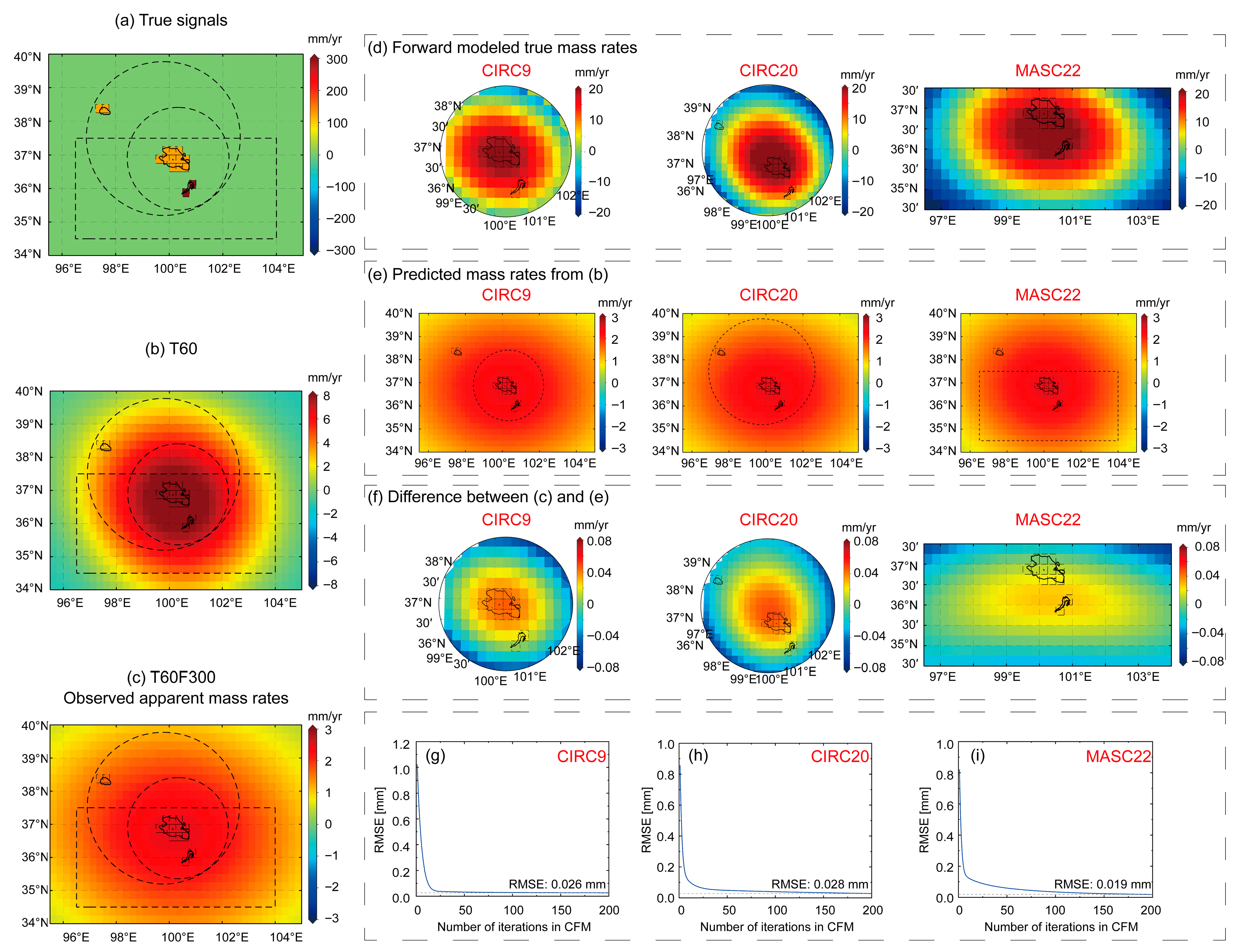
In the VSE, with equal mass changes in the three water bodies, Figure 5a–c illustrates that the signal center, after forward modeling, is primarily concentrated in the northwest of QHL. As the application of Fan filtering and the filtering radius increase, the regional signal disperses outward, reducing in strength (see Figure 5c,d). For instance, at the CIRC20 scale in the VSE, after forward modeling with T60, the original signal within the region retained a remaining signal ratio of 77.69% (see Figure 5b and

Table 2. LRWS changes, remaining signal ratio, and contribution ratio for four water body combinations under forward modeling with T60, T60F300, and T60F500 at three spatial scales.

Combined Methods	Contents	True (T0)			T60 (T1)			T60F300 (T2)			T60F500 (T3)
		CIRC9	CIRC20	MASC22	CIRC9	CIRC20	MASC22	CIRC9	CIRC20	MASC22	CIRC9	CIRC20	MASC22
ALL (A)	LRWS (A0, mm)	20.09	13.94	8.88	13.26	10.83	8.97	4.49	4.11	3.75	1.94	1.87	1.78
	RSR (Tn/T0)	-	-	-	66.00%	77.69%	100.95%	22.34%	29.52%	42.17%	9.64%	13.42%	20.06%
QHL (B)	LRWS (B0, mm)	10.04	4.65	4.44	5.97	4.51	3.81	1.73	1.52	1.43	0.69	0.65	0.63
	RSR (Tn/T0)	-	-	-	59.47%	96.98%	85.76%	17.22%	32.68%	32.19%	6.85%	14.03%	14.30%
	CR (B0/A0)	50.00%	33.33%	50.00%	45.05%	41.61%	42.47%	38.53%	36.91%	38.16%	35.50%	34.85%	35.63%
HLL (C)	LRWS (C0, mm)	0.00	4.65	0.00	1.99	3.00	0.97	1.14	1.29	0.81	0.58	0.61	0.50
	RSR (Tn/T0)	-	-	-	L-in	64.49%	L-in	L-in	27.87%	L-in	L-in	13.15%	L-in
	CR (C0/A0)	0.00%	33.33%	0.00%	15.00%	27.67%	10.86%	25.40%	31.47%	21.71%	30.03%	32.67%	27.99%
LYXR (D)	LRWS (D0, mm)	10.04	4.65	4.44	5.30	3.33	4.18	1.62	1.30	1.50	0.67	0.61	0.65
	RSR (Tn/T0)	-	-	-	52.73%	71.61%	94.21%	16.12%	28.00%	33.85%	6.65%	13.08%	14.60%
	CR (D0/A0)	50.00%	33.33%	50.00%	39.95%	30.72%	46.66%	36.07%	31.62%	40.13%	34.47%	32.48%	36.38%

Note: RSR denotes the remaining signal ratio; CR denotes the contribution ratio; the L-in denotes the signal within the study area results from leakage-in from external water bodies.

A). With the application of filtering methods, the remaining signal ratio dropped significantly to 29.52% (T60F300) and 13.42% (T60F500), respectively (see Figure 5c,d and Table 2 A). The forward modeling performed for a single water body reveals that, for the same mass change, the area of the water body and its distance from the study area’s center can affect its remaining signal ratio. For instance, at the CIRC20 scale, LYXR occupies a slightly larger spatial grid area than HLL and is located marginally closer to the center of the study area. Accordingly, its remaining signal ratio is higher than that of HLL after T60 or T60F300 filtering. Nevertheless, with increasing filtering radius, the effect of water body area becomes more pronounced than proximity to the study area center. As a result, under the T60F500 filtering condition, HLL exhibits a higher remaining signal ratio than LYXR (refer to Table 2 C and D).

This study examines the impact of external leakage-in signals when the water body is outside the study area. Under the spatial scales of CIRC9 and MASC22, where HLL is excluded, the leakage-in signals from HLL account for 15.00% (CIRC9) and 10.86% (MASC22) after forward modeling with T60 (see Figure 5j and Table 2 C). After applying filtering, the impact of leakage-in signals becomes more significant as the filtering radius increases (see Figure 5k,l). For instance, in the CIRC9 scale, after T60F300 and T60F500 processing, the contribution ratio of leakage-in signals reaches 25.40% and 30.03%, respectively (see Table 2 C). Conversely, at the MASC22 scale, after forward modeling with T60, the regional remaining signal ratio jointly modeled for the three water bodies reaches 100.95%, slightly exceeding the original signal by 0.09 mm (see Figure 5b and Table 2 A). This is primarily due to LYXR being near the center of MASC22, and MASC22 is large enough to retain most of the signals, with the remaining signal ratio being 94.21%. Additionally, at the MASC22 scale, HLL produces a leakage-in signal of 0.97 mm after forward modeling, contributing 10.86% to the regional signals of MASC22 (see Figure 5j and Table 2 C).

Overall, at three spatial scales, QHL and LYXR have a greater impact on the detection of regional TWS changes using gravimetric satellites. Nevertheless, at the scales of CIRC9 and MASC22, the influence of the leakage-in signals from HLL is substantial and further increases when filtering is applied with a larger radius.

3.2.2. Forward Modeling Using True Data

This study conducted the RSE forward modeling on three water bodies, using the long-term trend rates of actual monthly water storage change data in lakes and reservoirs from 2003 to 2022. The forward modeling with T60F500 was excluded from the experiment due to its strong attenuation of true signals, resulting in an extremely low remaining signal ratio. In the RSE, the central point of the forward modeled signal was concentrated closer to the center near QHL (Figure 6b,c). This concentration is mainly due to the larger water storage changes in QHL and LYXR compared to HLL. The impact of HLL on regional mass changes was greater in the VSE than in the RSE. For instance, at the CIRC9 scale, the contribution ratio of HLL leakage-in signal is 3.95% after T60 and 7.41% after T60F300 (see

Table 3. LRWS changes, remaining signal ratio, contribution ratio, and annual amplitude variation for four water body combinations under forward modeling with T60 and T60F300 at three spatial scales.

Combined Methods	Contents	True (T0)			T60 (T1)			T60F300 (T2)
		CIRC9	CIRC20	MASC22	CIRC9	CIRC20	MASC22	CIRC9	CIRC20	MASC22
ALL (A)	LRWS (A1, mm/yr)	12.60	6.52	5.57	7.52	5.63	5.07	2.30	2.01	1.94
	RSR (Tn/T0)	-	-	-	59.69%	86.34%	91.05%	18.22%	30.85%	34.89%
	Amplitude (mm)	24.7 ± 5.99	11.6 ± 2.85	10.9 ± 2.65	-	-	-	-	-	-
QHL (B)	LRWS (B1, mm/yr)	8.61	3.98	3.81	5.12	3.86	3.27	1.48	1.30	1.23
	RSR (Tn/T0)	-	-	-	59.47%	96.98%	85.76%	17.22%	32.68%	32.19%
	CR (B1/A1)	68.33%	61.07%	68.33%	60.47%	63.15%	54.76%	57.37%	58.61%	54.69%
	Amplitude (mm)	4.02 ± 2.71	1.86 ± 1.25	1.78 ± 1.20	-	-	-	-	-	-
HLL (C)	LRWS (C1, mm/yr)	0.00	0.69	0.00	0.30	0.45	0.15	0.17	0.19	0.12
	RSR (Tn/T0)	-	-	-	L-in	64.49%	L-in	L-in	27.87%	L-in
	CR (C1/A1)	0.00%	10.63%	0.00%	3.95%	7.94%	2.87%	7.41%	9.61%	6.24%
	Amplitude (mm)	-	0.34 ± 0.17	-	-	-	-	-	-	-
LYXR (D)	LRWS (D1, mm/yr)	3.99	1.85	1.76	2.10	1.32	1.66	0.64	0.52	0.60
	RSR (Tn/T0)	-	-	-	52.73%	71.61%	94.21%	16.12%	28.00%	33.85%
	CR (D1/A1)	31.67%	28.30%	31.67%	27.98%	23.47%	32.77%	28.02%	25.69%	30.72%
	Amplitude (mm)	20.9 ± 5.18	9.68 ± 2.40	9.26 ± 2.29	-	-	-	-	-	-

Note: RSR denotes the remaining signal ratio; CR denotes the contribution ratio; the L-in denotes the signal within the study area results from leakage-in from external water bodies; the “±” denotes the standard error.

C), both of which are lower than those in the previous VSE (>10%). At the MASC22 scale, the remaining signal ratio for the three water bodies together after forward modeling with T60 under the RSE (<100%) is lower than that under the VSE (>100%) because the impact of leakage-in signals from HLL based on true data is smaller than in VSE, with a leakage-in contribution ratio of only 2.87% (see Table 3 C).

At identical spatial scales and employing the same data-processing methods, the regional remaining signal ratio after forward modeling for the same individual water body is consistent in both RSE and VSE. Under these conditions, larger changes in the regional signal lead to greater signal loss. For example, in the case of QHL, the regional remaining signal ratio for both VSE and RSE is 32.68% at the CIRC20 scale after T60F300 processing. Nevertheless, the leakage-out signal is 3.13 mm for the VSE and 2.68 mm/yr for the RSE (see Table 2 B and Table 3 B). Therefore, VSE can somewhat reflect the impact of real water storage changes.

Furthermore, results indicate that the long-term trend signal contributed by QHL to the LRWS changes is greater than that contributed by the other two water bodies. Across the three spatial scales, the contribution of the QHL trend signal is nearly 2.15 times that of LYXR. For instance, at the CIRC20 scale, the long-term trend rate of LRWS changes is 6.52 mm/yr, with the contribution ratio by QHL being 61.07% (3.98 mm/yr), and that by LYXR being 28.30% (1.85 mm/yr, see Table 3 A, B, and D). Importantly, in terms of annual amplitude, the LRWS changes are more influenced by LYXR. The signal contribution of the amplitude of LYXR’s mass change is nearly 5.20 times that of QHL among the three spatial scales. For instance, at the CIRC20 scale, the annual amplitude of the LRWS changes is 11.6 ± 2.85 mm, with QHL and LYXR contributing 1.86 ± 1.25 mm and 9.68 ± 2.40 mm, respectively (see Table 3 A, B, and D).

The aforementioned forward modeling experiments revealed signal leakage in both the VSE and the RSE. As the signal source moves further from the study area center, the remaining signal ratio of a signal source with the same mass change decreases. Additionally, signal leakage-in from outside the region is also substantial. Figure 6a–c show the true signals of the area, and the spatial patterns observed by gravimetric satellites after T60 and T60F300 (Figure 6b,c), which differ from the original true signals (Figure 6a). As shown in Figure 6c–i, for the apparent mass rates obtained from the original true signals after T60F300 post-processing (Figure 6c), the CFM method was applied through 200 iterations at three spatial constraint scales (CIRC9, CIRC20, and MASC22) to recover the lost signals during the post-processing, resulting in the true mass changes simulated by forward modeling (Figure 6d). Figure 6c,e demonstrate that the apparent long-term water storage change rates (Figure 6c) and the predicted long-term water storage change rates (Figure 6e) exhibit good consistency in signal magnitude and spatial patterns, with minimal differences (see Figure 6f). The larger errors are primarily concentrated in certain edge regions. This phenomenon is mainly attributed to boundary effects induced by signals outside the iterative region, as well as the leakage of external signals into the interior of the iterative area [55]. Additionally, Figure 6g–i show the root mean square error (RMSE) between the apparent and predicted long-term water storage change rates at various spatial constraint scales. As the iteration progresses, the RMSE rapidly decreases and stabilizes at a low value. These results indicate that the CFM method can effectively recover attenuated signals.

3.3. Effectiveness of the CFM Method for GRACE/GRACE-FO Data

To recover the attenuated signals, the CFM method was applied to the SH solutions provided by CSR, JPL, and GFZ to derive corrected TWS changes under CIRC9, CIRC20, and MASC22 spatial constraint scales. Ensemble mean solutions are applied to decrease unknown noise in the gravity field [22,55]. At these three spatial scales, the mean recovered TWS changes across these SH solutions (hereafter referred to as “SH-CFM TWS”) were then compared with the mean TWS changes derived from the CSR- and GSFC-based Mascon solutions and with the corrected JPL Mascon solution (hereafter referred to as “Mascon TWS”) (see Figure 7). Ensemble mean was also applied to the corrected GWS changes derived from SH using the CFM method (hereafter referred to as “SH-CFM GWS”) and the Mascon GWS changes.

As shown in Figure 7, from 2003 to 2022, both SH-CFM and Mascon TWS changes consistently exhibited a long-term increasing trend across CIRC9, CIRC20, and MASC22 spatial scales. Moreover, the two TWS changes showed strong correlations at all three spatial scales, with correlation coefficients of 0.65 (CIRC9), 0.71 (CIRC20), and 0.82 (MASC22). The RMSE decreased significantly with increasing spatial scale. This indicates that the water storage changes derived from different GRACE/GRACE-FO post-processing methods exhibited reduced uncertainty and greater consistency at larger spatial scales. These results not only validate the stability of the Mascon method for large-scale water storage change inversion but also highlight the effectiveness of the CFM method underlying the SH solutions in capturing actual hydrological signals. It is worth noting that during the four periods marked by light gray backgrounds in Figure 7, the LYXR experienced several local peaks in water storage changes, demonstrating its artificial regulation function of “storing water during wet periods and releasing water during dry periods.” Nevertheless, a comparison of the response characteristics reveals that although Mascon TWS changes do respond to abrupt reservoir water storage changes, its ability to capture fine details is relatively limited, particularly in smaller-scale regions such as CIRC9. In contrast, SH-CFM TWS changes stand out by more sensitively capturing these abrupt signals across all scales, demonstrating a stronger responsiveness to hydrological events and an enhanced capability for anomaly identification.

Across three spatial scales, among the water storage components of TWS changes, the GWS component accounts for 39.95–43.44% and 31.17–44.05% of SH-CFM and Mascon TWS changes, respectively. The LRWS and SMS components account for 47.63–52.41% and 4.79–11.03% of TWS changes in the SH-CFM-based results, and 50.22–54.59% and 4.65–12.64% in the Mascon-based results, respectively (see Figure 8d–f). The trends of SWE and CWS components are relatively small (see Figure 8a–c), primarily due to regional geomorphic conditions, and their contributions to TWS changes are nearly negligible (see Figure 8d–f). As the spatial scale increases from CIRC9, CIRC20 to MASC22, the component exchange intensity derived from the SH-CFM-based and the Mascon-based results shows a decreasing trend (see Figure 8a–c). This trend is likely influenced by the distribution of permafrost across different spatial scales. As a unique aquitard, permafrost regulates the hydraulic connection between groundwater and surface water [60]. At smaller spatial scales, permafrost is discontinuously distributed with pronounced local heterogeneity: in some areas, groundwater and surface water interact frequently, whereas in others, permafrost forms barriers that restrict exchanges. This results in large phase differences among components, strong interactions, and consequently high component exchange intensity values. In contrast, at larger spatial scales, permafrost becomes more continuous and extensive, creating more uniform hydraulic barriers. When averaged over space, local phase differences are smoothed into a more coherent seasonal response, primarily driven by large-scale climatic variability such as seasonal precipitation. As a result, the component variations exhibit more synchronized seasonality, the interactions weaken, and the component exchange intensity decreases. The CCR ranges of GWS components derived from SH-CFM and Mascon methods are generally consistent across the three spatial scales. Similarly, the CCR ranges of LRWS components from both methods also show consistent ranges across these scales. This indicates that the main signals derived from SH-CFM and Mascon methods are similar in terms of seasonal amplitude and pattern [61], demonstrating the effectiveness of the CFM method in recovering the true signal.

Notably, the long-term trend of TWS changes at three spatial scales is lower than that of LRWS changes (see Figure 7 and Table 1). This is due to the combined impact of LRWS and GWS changes, which contribute over 85% to TWS changes at these scales (see Figure 8d–f), dominating the TWS change trends. From 2003 to 2022, GWS changes at the CIRC9, CIRC20, and MASC22 scales have declined significantly (see Figure 8a–c and

Table 4. The trend rates of GWS changes over the total period and three piecewise periods at the spatial scales of CIRC9, CIRC20, and MASC22.

Time	SH-CFM GWS [mm/yr]			Mascon GWS [mm/yr]
	CIRC9	CIRC20	MASC22	CIRC9	CIRC20	MASC22
200302–202212	−8.98 ± 0.52	−4.68 ± 0.32	−2.45 ± 0.34	−11.04 ± 0.33	−5.38 ± 0.16	−2.65 ± 0.16
200302–201209	−9.22 ± 1.24	−4.36 ± 0.75	−1.46 ± 0.72	−11.31 ± 1.10	−5.02 ± 0.51	−1.74 ± 0.46
201211–201705	−16.82 ± 4.66	−12.15 ± 2.42	−17.77 ± 2.45	−3.85 ± 2.31	−5.70 ± 1.30	−7.94 ± 1.36
201810–202212	−42.77 ± 5.39	−27.33 ± 3.21	−25.47 ± 3.18	−9.57 ± 2.30	−10.01 ± 1.46	−6.79 ± 1.45

Note: the “±” denotes the standard error.

). The decline at the CIRC20 scale (SH-CFM GWS: −0.94 ± 0.06 Gt/yr; Mascon GWS: −1.08 ± 0.03 Gt/yr) is close to the −0.96 ± 0.05 Gt/yr observed by Zhan et al. [22] for a similarly sized rectangular spatial area in the northeastern Tibetan Plateau from April 2002 to August 2020. The slight discrepancy reflects differences in study boundaries, time periods, and GRACE data processing algorithms [29]. Previous studies have not conducted comparisons of TWS changes at multiple spatial scales in this region, which is a key aspect of the present study. At the MASC22 scale, the decline in GWS changes observed in this study (SH-CFM GWS: −0.54 ± 0.07 Gt/yr; Mascon GWS: −0.58 ± 0.04 Gt/yr) is lower than that reported by Zhan et al. [22]. This is likely because our study focuses on the interaction between the adjacent lakes and reservoirs, neglecting the uncertain impact of rising water storage in Gyaring Lake and Ngoring Lake in the southwestern study area [7,22]. Regional TWS changes reflect variations in surface water and groundwater storage. In this study, GWS changes at the CIRC9 scale for both SH-CFM-based and Mascon-based results show the most significant decline, possibly due to groundwater converging into low-lying lakes and reservoirs. In summary, the continued depletion of regional groundwater and the ongoing rise in lake and reservoir water levels result in higher LRWS change rates compared to the TWS change rates.

The CFM method can effectively recover water storage signals from level-2 SH solutions, resulting in SH-CFM TWS that closely matches Mascon TWS across different spatial scales and is more sensitive to abrupt hydrological events. Therefore, the CFM method demonstrates strong effectiveness in restoring true hydrological signals and revealing regional terrestrial water storage dynamics.

3.4. Piecewise Periodic Changes of TWS and Its Water Storage Components

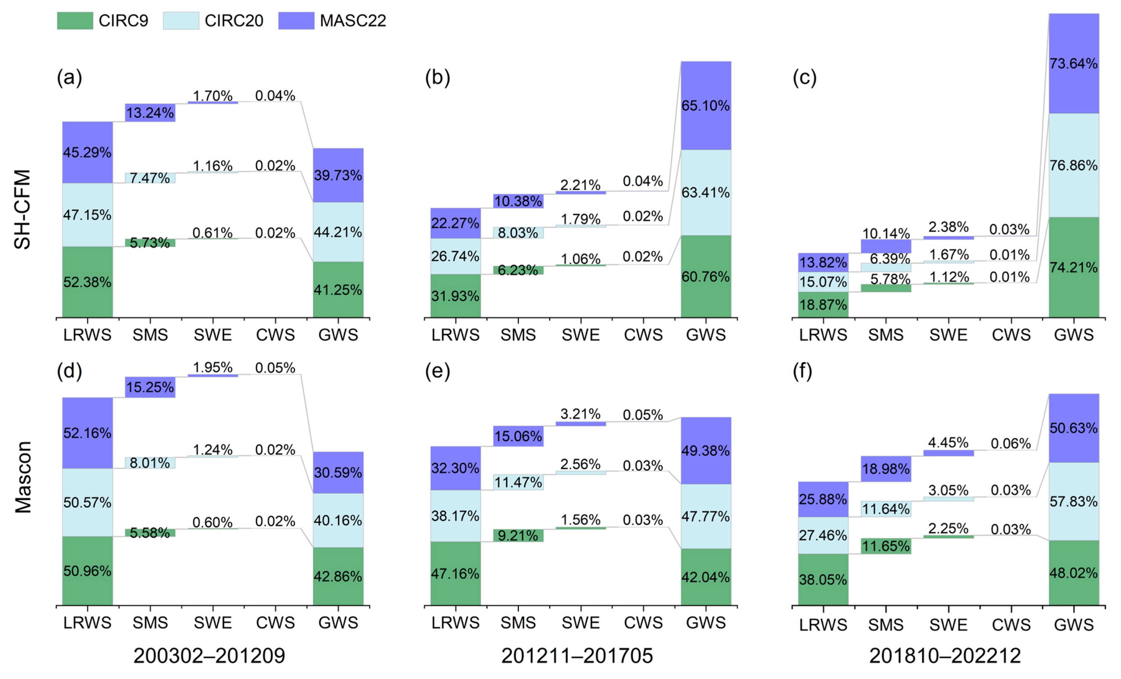
As shown in Figure 7, TWS changes over the northeastern Tibetan Plateau, influenced by fluctuations in lake and reservoir water storage, exhibit distinct phase characteristics across different piecewise periods, with alternating trends of increase and decrease. This pattern reflects the significant role of surface water bodies in regulating regional hydrological dynamics. The entire period 2003–2022 was divided into three different piecewise periods, i.e., January (February) 2003 to September 2012 (Piecewise period 1, where the starting month for GWS, SMS, SWE, and CWS changes is February), November 2012 to May 2017 (Piecewise period 2), and October 2018 to December 2022 (Piecewise period 3). The results indicate that during each piecewise period, SH-CFM and Mascon TWS changes exhibit similarly high correlations, and the RMSE decreases significantly as the spatial scale increases (

Table 5. SH-CFM and Mascon TWS change rates across multiple spatiotemporal scales, along with their correlation and RMSE.

Time	Methods	Trend [mm/yr]			Correlation Coefficients			RMSE [mm]
		CIRC9	CIRC20	MASC22	CIRC9	CIRC20	MASC22	CIRC9	CIRC20	MASC22
200301–201209	SH-CFM TWS	1.79 ± 1.16	1.09 ± 0.77	3.96 ± 0.95	0.49	0.66	0.83	29.57	16.86	16.70
	Mascon TWS	3.27 ± 0.51	2.41 ± 0.44	5.11 ± 0.60
201211–201705	SH-CFM TWS	−20.76 ± 4.42	−14.19 ± 2.52	−21.78 ± 2.57	0.65	0.80	0.84	41.77	19.34	24.08
	Mascon TWS	−10.03 ± 1.54	−8.06 ± 1.37	−11.61 ± 1.68
201810–202212	SH-CFM TWS	−47.31 ± 5.46	−30.07 ± 3.39	−29.31 ± 3.46	0.78	0.82	0.83	60.01	36.45	35.66
	Mascon TWS	−12.02 ± 1.93	−11.33 ± 1.62	−10.08 ± 1.92

Note: the “±” denotes the standard error.

). Figure 9 and

Table 6. The component exchange intensity of SH-CFM and Mascon TWS changes at the spatial scales of CIRC9, CIRC20, and MASC22 across three piecewise periods.

Time	Methods	CIRC9	CIRC20	MASC22
200302–201209	SH-CFM	0.67	0.61	0.44
	Mascon	0.84	0.72	0.52
201211–201705	SH-CFM	0.39	0.30	0.21
	Mascon	0.61	0.41	0.31
201810–202212	SH-CFM	0.20	0.17	0.18
	Mascon	0.53	0.39	0.37

show the CCR and component exchange intensity during the piecewise period for each storage component, respectively. Although LRWS and GWS changes were the primary contributors to TWS changes in the entire period 2003–2022, with largely consistent contributions (see Figure 8d–f), there were both similarities and differences in the contribution patterns of water storage components during the piecewise periods (see Figure 9).

In Piecewise period 1, LRWS and GWS changes remained the dominant contributing components to SH-CFM and Mascon TWS changes across the spatial scales of CIRC9, CIRC20, and MASC22. The contributions of each storage component were highly consistent with those observed during the entire period 2003–2022, and the component exchange intensity also remained essentially unchanged (see Figure 8 and Figure 9a,d, and Table 6). In contrast, in Piecewise periods 2 and 3, the contributions of each storage component to TWS changes varied significantly. During Piecewise period 2, SH-CFM and Mascon TWS changes exhibited a declining trend, with a strengthening in the CCR of GWS changes and a significant weakening in the CCR of LRWS changes (see Table 5 and Figure 9b,e). This may be attributable to the regulation of the LYXR. The abundant inflow in 2012 raised the reservoir to a high water level, but the subsequent inflow was insufficient, necessitating replenishment of the downstream basin. Consequently, the LRWS change rates shifted from increasing to decreasing, whereas GWS changes continued to decline (see Table 1 and Table 4). During Piecewise period 3, the downward trend of SH-CFM and Mascon TWS changes became more pronounced. The contribution of GWS changes to TWS changes further increased, and the contribution of LRWS changes further decreased (see Figure 9c,f). The significant decline in the CCR of LRWS changes is related to the design of the LYXR and the further depletion of groundwater. The abundant inflow in 2018 allowed the reservoir to reach its normal storage level for three consecutive years. Initially, the reservoir had a large water storage capacity, but once it reached the normal storage level, the storage could not increase further even if subsequent inflows were abundant, leading to stabilization or a slight decline in reservoir water storage changes. Therefore, although the water levels of QHL and HLL maintained an upward trend, the LRWS change trends were essentially stable, while the groundwater storage continued to decline (see Table 1 and Table 4). This also resulted in a continuous downward trend in TWS changes from October 2018 to December 2022 (see Table 5).

Furthermore, across the three piecewise periods, the component exchange intensity decreased during the latter two periods (see Table 6), indicating a weakening of the interaction intensity among the different water storage components. This trend may be associated with changes in water resources driven by climate change and human activities. Climate warming and the inducing permafrost degradation [13,62,63] promote and accelerate snowmelt recharge to soil moisture and groundwater, leading to a more in-phase alignment of the seasonal peaks of SWE, SMS, and GWS changes. Simultaneously, GWS changes exhibited a continuous declining trend, with an increased CCR (see Table 4 and Figure 9). Human activities, such as reservoir operations, have altered the natural hydrological cycle, and the relative contribution of LRWS changes has decreased, reducing the seasonal phase differences among components. Collectively, these factors weaken compensatory interactions among components, resulting in reduced component exchange intensity.

3.5. Dynamic Relationship Between Water Storage Components and Precipitation

This study investigates the relationship between TWS changes and their storage components with precipitation at three spatial scales. Cross-correlation analysis was performed to study the time lags between each water storage component and precipitation. Within a lag range of 0–6 months, the lag time corresponding to the maximum statistically significant correlation coefficient was selected. Figure 7 and Figure 8 illustrate the monthly precipitation variations and annual precipitation anomalies from 2003 to 2022, respectively, across three spatial scales. Despite the subtle positive precipitation anomaly in 2005, significant negative precipitation anomalies in previous years led to a pronounced response of the lake and reservoir to the 2005 anomaly. In response to significant positive precipitation anomalies observed in 2007, 2012, and 2018, LRWS consistently showed a reaction. Notably, the LYXR engaged in seasonal storage and discharge, fulfilling its role as a multi-year regulation reservoir (see Figure 4 and Figure 7). Except for CIRC9 with a 0-month lag, LRWS changes were significantly positively correlated with precipitation within a 0 to 6-month lag. At the CIRC9 scale, there was a 4-month lag, and at the CIRC20 and MASC22 scales, there was a 2-month lag (see

Table 7. The cross-correlation between TWS changes and its water storage components with precipitation at three spatial scales.

Spatial Scale	Time Lags [month]	LRWS	SMS	SWE	CWS	SH-CFM TWS	Mascon TWS	SH-CFM GWS	Mascon GWS
CIRC9	0	0.14	0.16 *	0.11	0.11	0.05	0.11	−0.11	−0.14
	1	0.17 *	0.20 *	0.07	−0.06	0.14 *	0.17 *	−0.07	−0.16 *
	2	0.17 *	0.14 *	0.07	−0.08	0.06	0.16 *	−0.12	−0.16 *
	3	0.16 *	0.09	0.03	−0.06	0.10	0.10	−0.07	−0.16 *
	4	0.18 *	0.11	0.09	0.01	0.08	0.11	−0.10	−0.18 *
	5	0.16 *	0.13	0.09	0.03	0.13	0.14	−0.05	−0.15 *
	6	0.18 *	0.13	0.01	0.04	0.17 *	0.19 *	−0.03	−0.15 *
CIRC20	0	0.14 *	0.21 *	0.11	0.13	0.09	0.12	−0.06	−0.13
	1	0.18 *	0.22 *	0.07	−0.07	0.17 *	0.20 *	−0.02	−0.13
	2	0.17 *	0.14 *	0.05	−0.09	0.10	0.17 *	−0.07	−0.13
	3	0.16 *	0.08	0.02	−0.07	0.12	0.12	−0.03	−0.14 *
	4	0.17 *	0.10	0.09	0.01	0.05	0.10	−0.11	−0.17 *
	5	0.16 *	0.13	0.07	0.03	0.11	0.13	−0.04	−0.14
	6	0.18 *	0.13	−0.02	0.04	0.15 *	0.20 *	−0.01	−0.11
MASC22	0	0.15 *	0.25 *	0.09	0.12	0.19 *	0.20 *	0.04	−0.05
	1	0.20 *	0.26 *	0.05	−0.06	0.27 *	0.26 *	0.12	−0.05
	2	0.19 *	0.20 *	0.07	−0.05	0.23 *	0.23 *	0.08	−0.05
	3	0.18 *	0.13	0.03	−0.04	0.19 *	0.16 *	0.07	−0.11
	4	0.19 *	0.15 *	0.11	0.00	0.14	0.16 *	−0.02	−0.14 *
	5	0.18 *	0.15 *	0.07	0.01	0.20 *	0.19 *	0.07	−0.09
	6	0.20 *	0.15 *	−0.01	0.01	0.20 *	0.23 *	0.06	−0.05

Note: * denotes significance at the 95% confidence level.

). This is primarily because, at smaller spatial scales dominated by QHL and the LYXR, lake and reservoir water bodies occupy a large proportion and exert a pronounced regulation effect. In particular, the anthropogenic operations of the LYXR cause a noticeable delay in the reservoir storage response to precipitation signals, and this delay effect is further propagated across the study area, which results in a slower response of the LRWS changes to precipitation inputs. At larger spatial scales, however, the proportion of non-reservoir areas increases, diluting the long lag effects caused by individual large reservoirs, so that the regional mean LRWS responds more rapidly to precipitation inputs. However, although SMS changes are not the primary contributor to TWS changes, they exhibit a more immediate response compared to LRWS changes, with an approximate 2-month lag following precipitation at three spatial scales (see Figure 8 and Table 7). The low but significant positive correlation between LRWS/SMS changes and precipitation may be influenced by artificial reservoir regulation, and uncertainties in land surface models regarding soil water simulation and soil depth selection in plateau regions [21,64]. At all three spatial scales, there was no significant correlation between SWE and CWS changes with precipitation within a 0 to 6-month lag (see Table 7), indicating that neither may be influenced by precipitation.

Notably, although the correlation between GWS changes and precipitation is not statistically significant, long-term GWS fluctuations are still influenced by precipitation variability. In particular, since 2018, a marked decrease in positive precipitation anomalies has been observed, accompanied by a persistent decline in GWS changes. This suggests that long-term precipitation trends have a substantial impact on the groundwater system.

SH-CFM TWS changes show a positive correlation with precipitation, similar to Mascon TWS changes. At smaller scales, precipitation has exerted a more temporally variable influence on water storage components like LRWS and SMS changes. Therefore, at the CIRC9 scale, precipitation with a 2- and 6-month lag significantly affects TWS changes. At the CIRC20 and MASC22 scales, both SH-CFM and Mascon TWS changes exhibit a 2-month lag relative to precipitation, indicating high consistency between the two methods in describing TWS changes (see Table 7). Overall, precipitation significantly impacts LRWS, SMS, and TWS changes, with more pronounced effects at larger scales (see Table 7).

4. Conclusions

This study revisited TWS changes in the northeastern Tibetan Plateau from 2003 to 2022 using GRACE/GRACE-FO at three spatial scales where large lakes and reservoirs coexist. The SH-CFM method was applied to correct the associated leakage errors and to recover the attenuated TWS signals. The main findings are as follows:

(1)

Large lakes and reservoirs exert a substantial influence on TWS changes in the northeastern Tibetan Plateau. The signals from QHL and LYXR, respectively, dominate the long-term trend and amplitude variations of LRWS changes, with LRWS contributing over 47% to TWS changes. Leakage errors are strongly affected by the surface area and location of water bodies, as well as the filtering radius.

(2)

From 2003 to 2022, both SH-CFM and Mascon TWS changes exhibited increasing trends across all three spatial scales. Long-term TWS changes are jointly governed by increasing LRWS and declining GWS, together explaining over 85% of the observed trends.

(3)

LRWS and SMS changes are significantly correlated with precipitation, typically exhibiting a 2–4-month lag, while GWS changes show weaker but long-term links. In addition, LRWS responds rapidly to pronounced positive precipitation anomalies. These relationships highlight the role of precipitation in modulating surface and subsurface water storage.

References

1. Tapley, B.D.; Bettadpur, S.; Watkins, M.; Reigber, C. The Gravity Recovery and Climate Experiment: Mission Overview and Early Results. Geophys. Res. Lett. 2004, 31, L09607. [Google Scholar] [CrossRef]
2. Landerer, F.W.; Flechtner, F.M.; Save, H.; Webb, F.H.; Bandikova, T.; Bertiger, W.I.; Bettadpur, S.V.; Byun, S.H.; Dahle, C.; Dobslaw, H.; et al. Extending the Global Mass Change Data Record: GRACE Follow-On Instrument and Science Data Performance. Geophys. Res. Lett. 2020, 47, e2020GL088306. [Google Scholar] [CrossRef]
3. Li, X.; Long, D.; Scanlon, B.R.; Mann, M.E.; Li, X.; Tian, F.; Sun, Z.; Wang, G. Climate change threatens terrestrial water storage over the Tibetan Plateau. Nat. Clim. Change 2022, 12, 801–807. [Google Scholar] [CrossRef]
4. Tapley, B.D.; Watkins, M.M.; Flechtner, F.; Reigber, C.; Bettadpur, S.; Rodell, M.; Sasgen, I.; Famiglietti, J.S.; Landerer, F.W.; Chambers, D.P.; et al. Contributions of GRACE to understanding climate change. Nat. Clim. Change 2019, 5, 358–369. [Google Scholar] [CrossRef]
5. Longuevergne, L.; Wilson, C.R.; Scanlon, B.R.; Crétaux, J.F. GRACE water storage estimates for the Middle East and other regions with significant reservoir and lake storage. Hydrol. Earth Syst. Sci. 2013, 17, 4817–4830. [Google Scholar] [CrossRef]
6. Carabajal, C.C.; Boy, J.-P. Lake and reservoir volume variations in South America from radar altimetry, ICESat laser altimetry, and GRACE time-variable gravity. Adv. Space Res. 2021, 68, 652–671. [Google Scholar] [CrossRef]
7. Yi, S.; Song, C.; Wang, Q.; Wang, L.; Heki, K.; Sun, W. The potential of GRACE gravimetry to detect the heavy rainfall-induced impoundment of a small reservoir in the upper Yellow River. Water Resour. Res. 2017, 53, 6562–6578. [Google Scholar] [CrossRef]
8. Wang, X.; de Linage, C.; Famiglietti, J.; Zender, C.S. Gravity Recovery and Climate Experiment (GRACE) detection of water storage changes in the Three Gorges Reservoir of China and comparison with in situ measurements. Water Resour Res. 2011, 47, W12502. [Google Scholar] [CrossRef]
9. Tong, X.; Pan, H.; Xie, H.; Xu, X.; Li, F.; Chen, L.; Luo, X.; Liu, S.; Chen, P.; Jin, Y. Estimating water volume variations in Lake Victoria over the past 22 years using multi-mission altimetry and remotely sensed images. Remote Sens. Environ. 2016, 187, 400–413. [Google Scholar] [CrossRef]
10. Li, X.; Tong, Z.; Wang, B.; Lei, S. Variation and Correlation Analysis of Lakewater Storage and Terrestrial Water Storage Anomaly in Poyang Lake. J. Yangtze River Sci. Res. Inst. 2023, 40, 38. [Google Scholar]
11. Xu, Y.; Li, J.; Wang, J.; Chen, J.; Liu, Y.; Ni, S.; Zhang, Z.; Ke, C. Assessing water storage changes of Lake Poyang from multi-mission satellite data and hydrological models. J. Hydrol. 2020, 590, 125229. [Google Scholar] [CrossRef]
12. Li, F.; Wang, Z.; Chao, N.; Song, Q. Assessing the Influence of the Three Gorges Dam on Hydrological Drought Using GRACE Data. Water. 2018, 10, 669. [Google Scholar] [CrossRef]
13. Zhang, G.; Yao, T.; Shum, C.K.; Yi, S.; Yang, K.; Xie, H.; Feng, W.; Bolch, T.; Wang, L.; Behrangi, A.; et al. Lake volume and groundwater storage variations in Tibetan Plateau’s endorheic basin. Geophys. Res. Lett. 2017, 44, 5550–5560. [Google Scholar] [CrossRef]
14. Rodell, M.; Li, B. Changing intensity of hydroclimatic extreme events revealed by GRACE and GRACE-FO. Nat. Water. 2023, 1, 241–248. [Google Scholar] [CrossRef]
15. Rodell, M.; Velicogna, I.; Famiglietti, J.S. Satellite-based estimates of groundwater depletion in India. Nature 2009, 460, 999–1002. [Google Scholar] [CrossRef] [PubMed]
16. Kim, H.; Yeh, P.J.F.; Oki, T.; Kanae, S. Role of rivers in the seasonal variations of terrestrial water storage over global basins. Geophys. Res. Lett. 2009, 36, L17402. [Google Scholar] [CrossRef]
17. Zhang, Y.F.; He, B.; Guo, L.L.; Liu, J.J.; Xie, X.M. The relative contributions of precipitation, evapotranspiration, and runoff to terrestrial water storage changes across 168 river basins. J. Hydrol. 2019, 579, 124194. [Google Scholar] [CrossRef]
18. Chao, N.; Li, F.; Yu, N.; Chen, G.; Wang, Z.; Ouyang, G.; Yeh, P.J. Divergent spatiotemporal variability of terrestrial water storage and eight hydroclimatic components over three different scales of the Yangtze River basin. Sci. Total Environ. 2023, 879, 162886. [Google Scholar] [CrossRef]
19. Zhang, G.; Chen, W.; Xie, H. Tibetan Plateau’s Lake Level and Volume Changes From NASA’s ICESat/ICESat-2 and Landsat Missions. Geophys. Res. Lett. 2019, 46, 13107–13118. [Google Scholar] [CrossRef]
20. Zhu, Z.; Fu, C.; Wu, H.; Wu, H.; Cao, Y.; Xia, Y. Decoding the hundred-year water level changes of the largest Saline Lake in China: A joint lake-basin modeling study based on a revised SWAT+. J. Hydrol. Reg. Stud. 2023, 49, 101521. [Google Scholar] [CrossRef]
21. Wang, L.; Chen, C.; Thomas, M.; Kaban, M.K.; Güntner, A.; Du, J. Increased water storage of Lake Qinghai during 2004–2012 from GRACE data, hydrological models, radar altimetry and in situ measurements. Geophys. J. Int. 2018, 212, 679–693. [Google Scholar] [CrossRef]
22. Zhan, P.; Song, C.; Luo, S.; Ke, L.; Liu, K.; Chen, T. Investigating different timescales of terrestrial water storage changes in the northeastern Tibetan Plateau. J. Hydrol. 2022, 608, 127608. [Google Scholar] [CrossRef]
23. Chen, J.; Li, J.; Zhang, Z.; Ni, S. Long-term groundwater variations in Northwest India from satellite gravity measurements. Glob. Planet. Change 2014, 116, 130–138. [Google Scholar] [CrossRef]
24. Chen, J.L.; Wilson, C.R.; Li, J.; Zhang, Z. Reducing leakage error in GRACE-observed long-term ice mass change: A case study in West Antarctica. J. Geod. 2015, 89, 925–940. [Google Scholar] [CrossRef]
25. Scanlon, B.R.; Longuevergne, L.; Long, D. Ground referencing GRACE satellite estimates of groundwater storage changes in the California Central Valley, USA. Water Resour. Res. 2012, 48, W04520. [Google Scholar] [CrossRef]
26. Famiglietti, J.S.; Lo, M.; Ho, S.L.; Bethune, J.; Anderson, K.J.; Syed, T.H.; Swenson, S.C.; de Linage, C.R.; Rodell, M. Satellites measure recent rates of groundwater depletion in California’s Central Valley. Geophys. Res. Lett. 2011, 38, L03403. [Google Scholar] [CrossRef]
27. Long, D.; Yang, Y.T.; Wada, Y.; Hong, Y.; Liang, W.; Chen, Y.N.; Yong, B.; Hou, A.Z.; Wei, J.F.; Chen, L. Deriving scaling factors using a global hydrological model to restore GRACE total water storage changes for China’s Yangtze River Basin. Remote Sens. Environ. 2015, 168, 177–193. [Google Scholar] [CrossRef]
28. Chen, J.L.; Wilson, C.R.; Tapley, B.D.; Save, H.; Cretaux, J.F. Long-term and seasonal Caspian Sea level change from satellite gravity and altimeter measurements. J. Geophys. Res. Solid Earth 2017, 122, 2274–2290. [Google Scholar] [CrossRef]
29. Long, D.; Chen, X.; Scanlon, B.R.; Wada, Y.; Hong, Y.; Singh, V.P.; Chen, Y.; Wang, C.; Han, Z.; Yang, W. Have GRACE satellites overestimated groundwater depletion in the Northwest India Aquifer? Sci. Rep. 2016, 6, 24398. [Google Scholar] [CrossRef] [PubMed]
30. Jiao, J.; Zhang, Y.; Bilker-Koivula, M.; Poutanen, M.; Yin, P.; Zhang, Y. Interannual glacier and lake mass changes over Scandinavia from GRACE. Geophys. J. Int. 2020, 221, 2126–2141. [Google Scholar] [CrossRef]
31. Ni, S.; Chen, J.; Wilson, C.; Hu, X. Long-Term Water Storage Changes of Lake Volta from GRACE and Satellite Altimetry and Connections with Regional Climate. Remote. Sens. 2017, 9, 842. [Google Scholar] [CrossRef]
32. Baoyin, Y.; Kezao, C.; Bowler, J.M.; Sujuan, Y. the Formation and Evolution of the Qinghai Lake. Quat. Sci. 1990, 10, 233–243. [Google Scholar]
33. Vishwakarma, B.; Devaraju, B.; Sneeuw, N. What is the spatial resolution of GRACE satellite products for hydrology? Remote Sens. 2018, 10, 852. [Google Scholar] [CrossRef]
34. Longuevergne, L.; Scanlon, B.R.; Wilson, C.R. GRACE Hydrological estimates for small basins: Evaluating processing approaches on the High Plains Aquifer, USA. Water Resour. Res. 2010, 46, W11517. [Google Scholar] [CrossRef]
35. Famiglietti, J.S.; Rodell, M. Water in the Balance. Science 2013, 340, 1300–1301. [Google Scholar] [CrossRef]
36. Save, H.; Bettadpur, S.; Tapley, B.D. High-resolution CSR GRACE RL05 mascons. J. Geophys. Res. Solid Earth 2016, 121, 7547–7569. [Google Scholar] [CrossRef]
37. Watkins, M.M.; Wiese, D.N.; Yuan, D.N.; Boening, C.; Landerer, F.W. Improved methods for observing Earth’s time variable mass distribution with GRACE using spherical cap mascons. J. Geophys. Res. Solid Earth 2015, 120, 2648–2671. [Google Scholar] [CrossRef]
38. Wiese, D.N.; Landerer, F.W.; Watkins, M.M. Quantifying and reducing leakage errors in the JPL RL05M GRACE mascon solution. Water Resour. Res. 2016, 52, 7490–7502. [Google Scholar] [CrossRef]
39. Loomis, B.D.; Luthcke, S.B.; Sabaka, T.J. Regularization and error characterization of GRACE mascons. J. Geod. 2019, 93, 1381–1398. [Google Scholar] [CrossRef]
40. Li, X.; Long, D.; Huang, Q.; Han, P.; Zhao, F.; Wada, Y. High-temporal-resolution water level and storage change data sets for lakes on the Tibetan Plateau during 2000–2017 using multiple altimetric missions and Landsat-derived lake shoreline positions. Earth Syst. Sci. Data. 2019, 11, 1603–1627. [Google Scholar] [CrossRef]
41. Rodell, M.; Houser, P.R.; Jambor, U.; Gottschalck, J.; Mitchell, K.; Meng, C.J.; Arsenault, K.; Cosgrove, B.; Radakovich, J.; Bosilovich, M.; et al. The Global Land Data Assimilation System. Bull. Am. Meteorol. Soc. 2004, 85, 381–394. [Google Scholar] [CrossRef]
42. Li, B.; Rodell, M.; Kumar, S.; Beaudoing, H.K.; Getirana, A.; Zaitchik, B.F.; de Goncalves, L.G.; Cossetin, C.; Bhanja, S.; Mukherjee, A.; et al. Global GRACE Data Assimilation for Groundwater and Drought Monitoring: Advances and Challenges. Water Resour. Res. 2019, 55, 7564–7586. [Google Scholar] [CrossRef]
43. Zhang, G.Q.; Yao, T.D.; Chen, W.F.; Zheng, G.X.; Shum, C.K.; Yang, K.; Piao, S.L.; Sheng, Y.W.; Yi, S.; Li, J.L.; et al. Regional differences of lake evolution across China during 1960s-2015 and its natural and anthropogenic causes. Remote Sens. Environ. 2019, 221, 386–404. [Google Scholar] [CrossRef]
44. Yang, K.; Lu, H.; Yue, S.Y.; Zhang, G.Q.; Lei, Y.B.; La, Z.; Wang, W. Quantifying recent precipitation change and predicting lake expansion in the Inner Tibetan Plateau. Clim. Change 2018, 147, 149–163. [Google Scholar] [CrossRef]
45. Ni, S.N.; Chen, J.L.; Wilson, C.R.; Li, J.; Hu, X.G.; Fu, R. Global Terrestrial Water Storage Changes and Connections to ENSO Events. Surv. Geophys. 2018, 39, 1–22. [Google Scholar] [CrossRef]
46. Wahr, J.; Molenaar, M.; Bryan, F. Time variability of the Earth’s gravity field: Hydrological and oceanic effects and their possible detection using GRACE. J. Geophys. Res. Solid. Earth. 1998, 103, 30205–30229. [Google Scholar] [CrossRef]
47. Swenson, S.; Chambers, D.; Wahr, J. Estimating geocenter variations from a combination of GRACE and ocean model output. J. Geophys. Res. Soli. Earth. 2008, 113, B08410. [Google Scholar] [CrossRef]
48. Jin, S.; Zhang, L.J.; Tapley, B.D. The understanding of length-of-day variations from satellite gravity and laser ranging measurements. Geophys. J. Int. 2011, 184, 651–660. [Google Scholar] [CrossRef]
49. Cheng, M.; Tapley, B.D.; Ries, J.C. Deceleration in the Earth’s oblateness. J. Geophys. Res. Solid. Earth. 2013, 118, 740–747. [Google Scholar] [CrossRef]
50. Geruo, A.; Wahr, J.; Zhong, S. Computations of the viscoelastic response of a 3-D compressible Earth to surface loading: An application to Glacial Isostatic Adjustment in Antarctica and Canada. Geophys. J. Int. 2012, 192, 557–572. [Google Scholar] [CrossRef]
51. Zhang, Z.-Z.; Chao, B.F.; Lu, Y.; Hsu, H.-T. An effective filtering for GRACE time-variable gravity: Fan filter. Geophys. Res. Lett. 2009, 36, L17311. [Google Scholar] [CrossRef]
52. Chambers, D.P. Evaluation of new GRACE time-variable gravity data over the ocean. Geophys. Res. Lett. 2006, 33, L17603. [Google Scholar] [CrossRef]
53. Chen, J.; Ries, J.C.; Tapley, B.D. Assessment of degree-2 order-1 gravitational changes from GRACE and GRACE Follow-on, Earth rotation, satellite laser ranging, and models. J. Geod. 2021, 95, 38. [Google Scholar] [CrossRef]
54. Zou, Y.; Kuang, X.; Feng, Y.; Jiao, J.J.; Liu, J.; Wang, C.; Fan, L.; Wang, Q.; Chen, J.; Ji, F.; et al. Solid Water Melt Dominates the Increase of Total Groundwater Storage in the Tibetan Plateau. Geophys. Res. Lett. 2022, 49, e2022GL100092. [Google Scholar] [CrossRef]
55. Zhang, G.Q.; Shen, W.B.; Fu, G.Y.; Li, Z.J.; Zhu, Y.Q.; Wang, Y. Moho Changes Beneath the Northeastern Tibetan Plateau Revealed by Multiple Geodetic Datasets. J. Geophys. Res. -Solid. Earth. 2021, 126, e2021JB022060. [Google Scholar] [CrossRef]
56. Tan, Q. The Longyangxia Reservoir on the Yellow River Has Reached Its Highest Water Level in 19 Years Since the Construction of the Dam. Available online: https://news.sina.com.cn/c/2005-10-09/11397956956.shtml (accessed on 12 June 2025).
57. Liu, C.; Wang, S. Artificial Rain Enhancement Enriches Water Sources, Restoring the Clear, Rippling Waters of Longyangxia Reservoir. Available online: https://news.sina.com.cn/c/2003-09-11/1859734565s.shtml (accessed on 12 June 2025).
58. Zhang, Y.; Fu, Y.; Dai, S. The Water Surface Area of the Longyangxia Reservoir Area Increased Significantly in 2005. Available online: https://news.sina.com.cn/c/p/2005-08-30/18027635098.shtml (accessed on 12 June 2025).
59. Ge, X.; Zhang, Q. The Longtou Hydropower Station on the Yellow River Has Been in Operation for 31 Years, and the Reservoir Level Has Reached the Normal Storage Level for the First Time. Available online: http://news.cnr.cn/native/city/20181106/t20181106_524406393.shtml (accessed on 12 June 2025).
60. Xu, M.; Kang, S.; Zhao, Q.; Li, J. Terrestrial Water Storage Changes of Permafrost in the Three-River Source Region of the Tibetan Plateau, China. Adv. Meteorol. 2016, 2016, 4364738. [Google Scholar] [CrossRef]
61. Huang, Z.; Yeh, P.J.F.; Pan, Y.; Jiao, J.J.; Gong, H.; Li, X.; Güntner, A.; Zhu, Y.; Zhang, C.; Zheng, L. Detection of large-scale groundwater storage variability over the karstic regions in Southwest China. J. Hydrol. 2019, 569, 409–422. [Google Scholar] [CrossRef]
62. Huang, J.P.; Zhou, X.J.; Wu, G.X.; Xu, X.D.; Zhao, Q.Y.; Liu, Y.M.; Duan, A.M.; Xie, Y.K.; Ma, Y.M.; Zhao, P.; et al. Global Climate Impacts of Land-Surface and Atmospheric Processes Over the Tibetan Plateau. Rev. Geophys. 2023, 61, e2022RG000771. [Google Scholar] [CrossRef]
63. Guo, D.; Wang, H.; Li, D. A projection of permafrost degradation on the Tibetan Plateau during the 21st century. J. Geophys. Res. Atmos. 2012, 117, D05106. [Google Scholar] [CrossRef]
64. Bi, H.; Ma, J.; Zheng, W.; Zeng, J. Comparison of soil moisture in GLDAS model simulations and in situ observations over the Tibetan Plateau. J. Geophys. Res. Atmos. 2016, 121, 2658–2678. [Google Scholar] [CrossRef]
Figure 1. Spatial distribution of lake, reservoir, and study scales in the northeastern Tibetan Plateau. The black grids at 0.25 degrees represent the spatial extent used for forward modeling.
Remotesensing 17 03272 g001
Figure 2. Flow chart with the major methodology and processing in this study.
Remotesensing 17 03272 g002
Figure 3. The relationship between water level and water storage changes in QHL, HLL, and LYXR. (a) Relationship for QHL; (b) Relationship for HLL; (c) Relationship for LYXR. The colored markers at the bottom represent the 95% confidence intervals of the fitted results.
Remotesensing 17 03272 g003
Figure 4. (a) Water storage changes of QHL, HLL, and LYXR from 2003 to 2022; (b) Water storage changes of QHL derived from the Hydroweb database and in situ measurements of the water storage at the Xiashe station. (c) LRWS changes at different spatial scales, including CIRC9, CIRC20, and MASC22. Note: the “±” denotes the standard error.
Remotesensing 17 03272 g004
Figure 5. Forward modeling results for the VSE. A volume of 1-km3 of water was distributed over the gridded extent (0.25-degree resolution) for QHL, HLL, and LYXR. The spatial distribution of the signals was obtained by forward modeling with T60, T60F300, and T60F500. Four scenarios were considered: the three water bodies together and each water body individually. (ad) The results of forward modeling for QHL, HLL, and LYXR; (eh) The results of forward modeling for QHL; (il) The results of forward modeling for HLL; (mp) The results of forward modeling for LYXR.
Remotesensing 17 03272 g005
Figure 6. Forward modeling results for the RSE and the corrected results based on the CFM method. (a) Long-term LRWS change rates from 2003 to 2022; (b) Apparent long-term LRWS change rates after T60; (c) Apparent long-term LRWS change rates after T60F300; (d) “True” long-term LRWS change rates recovered by the CFM method after 200 iterations; (e) Predicted long-term LRWS change rates derived from (d) after T60F300; (f) Difference between the apparent and predicted long-term LRWS change rates (i.e., (ce)). Please note the different color scale ranges in the subplots. The three columns in (d), (e), and (f) correspond to the spatial constraint scales of CIRC9, CIRC20, and MASC22, respectively. (gi) show the residuals change between the (c,e) for the corresponding spatial constraint scales. The residuals are calculated as the root mean square error of the differences between the (c,e) at each grid point within the corresponding constraint range.
Remotesensing 17 03272 g006
Figure 7. The SH-CFM TWS, Mascon TWS, and LYXR water storage changes under the spatial scales of CIRC9, CIRC20, and MASC22, respectively, as well as the monthly precipitation from GPCC. Note: The shaded region of the TWS changes curve represents the standard deviation for the mean values of different solutions, while the “±” denotes the standard error. The four vertically shaded light gray periods indicate multiple local peaks in LYXR water storage changes.
Remotesensing 17 03272 g007
Figure 8. (ac): GWS, SMS, SWE, and CWS changes at three spatial scales (CIRC9, CIRC20, MASC22), along with component exchange intensity and annual precipitation anomalies. (df): CCR of each TWS component, with outer and inner rings indicating SH-CFM-based and Mascon-based results, respectively. Note: Percentages may not add up to 100% due to rounding.
Remotesensing 17 03272 g008
Figure 9. CCR of water storage components to SH-CFM and Mascon TWS changes at different spatial scales across three piecewise periods: (a,d) February 2003 to September 2012, (b,e) November 2012 to May 2017, and (c,f) October 2018 to December 2022, with SH-CFM-based results in (ac) and Mascon-based results in (df). Note: Percentages may not add up to 100% due to rounding.
Remotesensing 17 03272 g009