Article

HSSTN: A Hybrid Spectral–Structural Transformer Network for High-Fidelity Pansharpening

1
Department of Electronic Information, Rocket Force University of Engineering, Xi’an 710025, China
2
School of Automation, China University of Geosciences, Wuhan 430074, China
3
School of Information Engineering, Zhongnan University of Economics and Law, Wuhan 430073, China
4
Engineering Research Center of Natural Resource Information Management and Digital Twin Engineering Software, Ministry of Education, Wuhan 430074, China
5
Hubei Key Laboratory of Intelligent Geo-Information Processing, China University of Geosciences, Wuhan 430074, China
*
Author to whom correspondence should be addressed.
Remote Sens. 2025, 17(19), 3271; https://doi.org/10.3390/rs17193271
Submission received: 30 July 2025 / Revised: 20 September 2025 / Accepted: 22 September 2025 / Published: 23 September 2025
(This article belongs to the Special Issue Artificial Intelligence in Hyperspectral Remote Sensing Data Analysis)

Abstract

Highlights

What are the main findings?
  • A Hybrid Spectral–Structural Transformer Network (HSSTN) is proposed, using an asymmetric architecture and hierarchical fusion to reduce spectral distortion and spatial degradation.
  • The proposed HSSTN demonstrates state-of-the-art performance on multiple satellite datasets, outperforming eleven advanced methods in both quantitative metrics and visual quality with sharper details and fewer artefacts.
What are the implications of the main findings?
  • This study confirms that an asymmetric, hybrid architecture tailored to different data modalities is a highly effective strategy to overcome the inherent performance trade-offs of single-paradigm models, successfully resolving the core conflict between spatial detail enhancement and spectral fidelity.
  • The proposed hierarchical fusion network provides a flexible and powerful blueprint for integrating features from heterogeneous remote sensing sources. This progressive fusion approach offers a promising pathway for developing more robust multimodal and multi-scale models in the future.

Abstract

Pansharpening fuses multispectral (MS) and panchromatic (PAN) remote sensing images to generate outputs with high spatial resolution and spectral fidelity. Nevertheless, conventional methods relying primarily on convolutional neural networks or unimodal fusion strategies frequently fail to bridge the sensor modality gap between MS and PAN data. Consequently, spectral distortion and spatial degradation often occur, limiting high-precision downstream applications. To address these issues, this work proposes a Hybrid Spectral–Structural Transformer Network (HSSTN) that enhances multi-level collaboration through comprehensive modelling of spectral–structural feature complementarity. Specifically, the HSSTN implements a three-tier fusion framework. First, an asymmetric dual-stream feature extractor employs a residual block with channel attention (RBCA) in the MS branch to strengthen spectral representation, while a Transformer architecture in the PAN branch extracts high-frequency spatial details, thereby reducing modality discrepancy at the input stage. Subsequently, a target-driven hierarchical fusion network utilises progressive crossmodal attention across scales, ranging from local textures to multi-scale structures, to enable efficient spectral–structural aggregation. Finally, a novel collaborative optimisation loss function preserves spectral integrity while enhancing structural details. Comprehensive experiments conducted on QuickBird, GaoFen-2, and WorldView-3 datasets demonstrate that HSSTN outperforms existing methods in both quantitative metrics and visual quality. Consequently, the resulting images exhibit sharper details and fewer spectral artefacts, showcasing significant advantages in high-fidelity remote sensing image fusion.

1. Introduction

Amid global digital transformation and rapid technological change, infrastructure modernisation is now central to national development. Remote sensing satellites, as key components of space-based infrastructure, are vital for strategic needs, including resource exploration, urban planning, military uses, and climate change monitoring [1,2,3,4].
Many remote sensing satellites are in orbit, such as QuickBird, Gaofen-1, Gaofen-2, and WorldView-3. However, satellite sensors cannot capture images with both high spectral and spatial resolution from a single platform [5,6]. To address this, pansharpening of multispectral imagery enables high spatial–spectral resolution in remote sensing images. This technique has long been a significant research focus [7,8].
The genesis of pansharpening techniques dates to 1985 when Cliche et al. [9] first enhanced multispectral image spatial resolution using panchromatic image components, substantially improving SPOT-1 satellite imagery’s observational accuracy. This seminal work established the foundation for remote sensing image pansharpening research. To date, diverse methodologies have been developed to address this challenge, with pixel-level fusion emerging as the prevailing paradigm [10,11]. This approach involves creating new images through pixel-by-pixel integration of input data, and existing methods are principally categorised into traditional and deep learning groups.
Traditional pansharpening methods are principally categorised into three classes: Component Substitution (CS), Multi-Resolution Analysis (MRA), and Variational Optimisation (VO). CS methods exhibit high computational efficiency and strong spatial detail preservation, yet remain susceptible to spectral distortion under low correlation between panchromatic (PAN) and multispectral (MS) imagery [12,13]. MRA methods achieve high spectral fidelity but introduce spatial artefacts, demonstrate registration sensitivity, and require higher computational complexity [14,15]. VO approaches formulate pansharpening as mathematical optimisation problems, though their substantial computational overhead persists as a primary constraint [16,17].
Owing to their powerful nonlinear fitting capabilities and robust multi-level feature extraction, deep learning methods have revolutionised diverse image processing tasks. Following the seminal 2016 work by Masi et al. [18], deep-learning-based approaches rapidly became the de facto standard for pansharpening. Early research in this domain predominantly focused on developing more complex convolutional neural network (CNN) architectures to enhance fusion performance. Specifically, advances progressed along multiple dimensions; some studies designed dedicated networks to improve spectral prediction [19], while others concentrated on extracting more comprehensive features. For instance, Ye et al. [20] explored multi-scale convolutional kernels to capture richer and more diverse image information.
However, researchers soon recognised that treating MS and PAN imagery as homogeneous inputs ignored their inherent modal differences. To address this, Liu et al. [21] pioneered a dual-stream fusion network processing MS and PAN data through separate branches. Building on this, Yong et al. [22] incorporated channel and spatial attention mechanisms [23] to enable adaptive learning and enhancement of critical features per modality. Extending this concept, Wang et al. [24] designed an Adaptive Feature Fusion Module (AFFM) that reduces inter-branch redundancy while promoting complementarity via learned weight maps. Despite continuous evolution of these CNN-based methods, they remain constrained by a fundamental bottleneck: the limited receptive fields of convolutional operations. This results in deficient global context modelling and long-range dependency capture, particularly manifesting as suboptimal performance when processing large-scale homogeneous regions or restoring complex structures.
Consequently, to overcome the limitations of CNN in global modelling, Transformer architectures migrated from natural language processing to computer vision. Particularly, the Vision Transformer (ViT) pioneered the core self-attention mechanism [25], which effectively captures long-range dependencies among image patches and establishes an alternative paradigm for crossmodal feature modelling in pansharpening.
The application of this paradigm to pansharpening was pioneered by Zhou et al. [26] via Panformer. Subsequently, works like HyperTransformer [27] further explored Transformer’s potential for multi-scale, long-range detail capture. Later research pursued more sophisticated applications, constructing dual-branch multi-scale networks with independent spatial/spectral Transformers for comprehensive information capture [28], or employing mutual information-based Transformers to decouple shared and sensor-specific features [29]. Concurrently, a critical consensus emerged that pure Transformer models may underperform compared to CNNs in extracting fine-grained local textures regarding efficiency and effectiveness. This insight spurred hybrid architecture research. For instance, Li et al. [30] integrated Transformers with shallow CNNs to leverage local feature extraction capabilities; alternatively, frequency-domain analysis incorporating Discrete Wavelet Transform (DWT) for feature separation has been combined with Transformer-based bijective functions for refined fusion [31].
In summary, notwithstanding the considerable advancement achieved in prevailing methodologies, pansharpening continues to grapple with two intrinsic challenges. Firstly, the inherent limitations of single-model paradigms must be taken into consideration. CNN-based methods demonstrate proficiency in local detail extraction; however, they encounter difficulties with global context modelling. Conversely, Transformer-based approaches effectively capture global relationships; however, their patch-based processing can disrupt fine-grained local textures, and the quadratic complexity of global self-attention poses a significant computational burden for high-resolution imagery. Secondly, contemporary models often fail to strike a balance between preserving spectral fidelity and introducing spatial detail. The enhancement of spatial details to an excessive degree risks severe spectral distortion, whereas an overemphasis on spectral fidelity may compromise spatial sharpness, yielding blurred imagery.
In order to address these challenges, a Hierarchical Spectral–Structural Transformer Network (HSSTN) is proposed, which enables three-level synergistic enhancement for pansharpening. The core design employs a hierarchical enhancement strategy inspired by the divide-and-conquer principle, assigning distinct optimisation targets to each stage: detail focus at shallow levels, structural emphasis at mid-levels, and global context modelling at deep levels. This strategy is employed to specifically optimise spectral, structural, and detailed features. The primary contributions of this study are as follows:
  • A novel end-to-end pansharpening framework, the Hierarchical Spectral–Structural Transformer Network (HSSTN), is proposed. The HSSTN is built upon a three-stage synergistic enhancement strategy, comprising an asymmetric dual-stream encoder, a hierarchical fusion network, and a multi-objective loss function to ensure a balanced restoration of spectral and spatial information.
  • An asymmetric architecture is designed to address the inherent modality gap between PAN and MS imagery. It includes a dual-stream encoder that assigns specialised pathways for PAN and MS data. The PAN branch uses a pure Transformer to maximise spatial detail extraction, while the MS branch employs a hybrid CNN–Transformer design to prioritise spectral preservation before contextual modelling. A hierarchical fusion network that progressively integrates these optimised features, moving from fine-grained detail injection to multi-scale structural aggregation, thereby ensures controlled spatial enhancement while mitigating spectral distortion.
  • A synergistic optimisation framework is introduced via a multi-objective loss function. This loss function simultaneously constrains pixel-level fidelity (L1), structural similarity (SSIM), and global spectral integrity (ERGAS), guiding the network to achieve a comprehensive and balanced optimisation across all critical quality metrics during the training process.
The outline of this paper is organised as follows: In Section 2, we will briefly introduce the related work. Section 3 introduces our proposed method, detailing the network architecture adopted in this work. Section 4 details and discusses the conducted experiments, including the datasets, evaluation metrics, experimental environment, and results. Section 5 discusses the experiments of this paper, analyzing the experimental results. Finally, Section 6 summarises the key findings and conclusions of this study.

2. Related Work

2.1. Supervised Pansharpening

Supervised methods are the mainstream of current research. They rely on ground truth (GT) information to perform pansharpening, following Wald’s protocol [32]. In this protocol, the MS image and PAN image are downsampled, with the original MS image serving as the simulated GT image. Masi et al. [18] first proposed a pansharpening model called PNN based on convolutional neural networks. Subsequent studies expanded network depth and breadth; Yuan et al. [33] proposed MSDCNN, which uses convolution kernels of different sizes to capture image features, while Yang et al. [34] introduced PanNet, improving generalisation by training in the high-frequency domain. To better handle modal differences, Liu et al. [21] proposed a dual-stream network (TFNet). More advanced architectures combine deep learning with classical principles, such as model-guided cross-fusion networks that unfold spectral and imaging priors into distinct sub-networks for collaborative optimisation [35], and methods that integrate traditional regularisation, such as using a generalised tensor nuclear norm (GTNN) to impose low-rank constraints within a supervised framework [36]. Concurrently, with the widespread application of generative adversarial networks (GANs), Liu et al. [37] proposed PSGAN, using a dual-branch network as the generator to enhance perceptual quality.
With the success of Transformers in computer vision, researchers began to introduce them into pansharpening to better model long-range dependencies. Zhou et al. [26] pioneered this direction with PanFormer. A significant research thrust within this paradigm involves exploring the low-rank characteristics of remote sensing data. This has led to the development of low-rank Transformer networks for high-resolution computational imaging [38], and deep reconstruction networks that leverage low-rank tensor representations (LTRNs) to effectively learn image priors [39]. In contrast to these attention-based approaches, He et al. [40] proposed Pan-Mamba, a method based on the state-space model that leverages Mamba’s advantages in global information modelling. Although these supervised methods perform well, they often face challenges in balancing spectral fidelity and spatial detail injection, which motivates the exploration of more refined network architectures.

2.2. Unsupervised Pansharpening

In response to the challenges of supervised methods, particularly their reliance on synthetic training data and potential generalisation issues, unsupervised learning frameworks have emerged as a significant alternative. These methods directly capture spectral and spatial information from the original scale of the images [41], operating without GT information and instead adhering to the consistency principle of Wald’s protocol. The core idea is to train the network by enforcing spectral consistency between the downsampled fused image and the original MS image and spatial consistency between the fused image and the original PAN image. A key element of this paradigm is the design of no-reference loss functions that effectively balance these two constraints [42].
Early explorations in this area focused on CNN architectures. Luo et al. [43] introduced an iterative CNN with multiple skip connections, applying a feature guidance strategy to improve information reuse. To further refine feature extraction, Xiong et al. [44] introduced UAP-Net, which uses a residual network and a spatial texture attention block to enhance high-frequency details. Ni et al. [45] proposed a pansharpening network (LDP-Net), which includes a KL loss to enhance spatial and spectral consistency. Other approaches, like the guided deep decoder proposed by Uezato et al. [46], treat fusion as a general problem and optimise network parameters in an unsupervised manner using a guidance image.
Subsequently, generative adversarial networks (GANs) were applied to unsupervised pansharpening. Ma et al. [47] proposed the first unsupervised GAN method, Pan-GAN, which employs spectral and spatial discriminators for adversarial training. Following this, Zhou et al. [48] proposed PGMAN, which employs a similar framework. More recent and advanced paradigms have also been explored. Dian et al. [49] introduced a zero-shot learning (ZSL) method that first estimates sensor characteristics to better generalise to test data. Furthermore, leveraging the power of advanced generative models, Rui et al. [50] proposed a low-rank diffusion model (PLRDiff) for pansharpening, combining a pre-trained diffusion model with the Bayesian method to improve generalisation ability.
Despite different training paradigms, both supervised and unsupervised methods face the core challenge of efficiently handling the modality differences between PAN and MS images. Early deep learning models typically combine the upsampled MS and PAN images through concatenation or addition and then feed them into a single convolutional neural network for feature extraction and fusion [18,33], as shown in Figure 1a,b. The main advantage of this design is its simplicity. However, it treats two very different types of images as if they are the same. This can lead to mixed-up features, making it hard for the model to learn the unique characteristics of each image. As a result, this often causes spectral distortion and blurry spatial details.
To solve this problem, the dual-stream architecture was introduced, as shown in Figure 1c. Researchers designed separate feature extraction branches for PAN and MS images. This allowed the network to learn features specific to each modality, providing higher-quality inputs for the later fusion stage and significantly improving performance. However, many existing dual-stream networks are still functionally homogeneous, even if their branches have different depths or numbers of modules [21,26,37,40]. They might use the same type of convolutional or Transformer blocks in both branches as general-purpose feature extractors. While this strategy is better than the single-stream approach, it does not fundamentally provide specialised designs for the rich spatial structures of PAN images and the fine spectral properties of MS images. This limitation restricts further improvements in fusion performance.
Consequently, structural asymmetry in itself is inadequate for resolving the modality difference problem. In order to address this issue, it is proposed that independent encoding branches be provided for PAN and MS images. Each branch would be assigned a completely different functional mission and module design (see Figure 1d). The two branches of the algorithm are able to extract the feature information of the images and take into account the differences and correlations between them.

3. Proposed Methods

In this section, the proposed HSSTN is presented. The proposed method is outlined in Section 3.1. Section 3.2 provides a comprehensive overview of the dual-stream feature extractor. In the following section, referred to as Section 3.3, a thorough account of the hierarchical fusion network is provided. Furthermore, the multi-objective collaborative optimisation loss is delineated in Section 3.4.

3.1. Overview of the Proposed Approach

Inspired by the divide-and-conquer principle, the HSSTN employs a hierarchical synergistic enhancement strategy to comprehensively optimise spectral, structural, and detailed features. Specifically, the proposed methodology comprises three key components: a dual-stream feature extractor, a hierarchical fusion network, and an image reconstruction head, as demonstrated in Figure 2. In this approach, the resolution of the intrinsic conflict between preserving spectral fidelity and enhancing spatial detail in pansharpening is achieved through the Hybrid Spectral–Structural Transformer Network.
In the HSSTN, an asymmetric dual-stream feature extractor is implemented, with customised encoding paths for MS and PAN imagery. Specifically, the panchromatic detail stream encoder employs a pure Transformer architecture to optimise high-frequency spatial detail extraction, while the MS-RBCA spectral encoder integrates a CNN-based channel attention module (RBCA) with Transformer Self-Attention Blocks (SABs). This configuration preserves key spectral information during the initial encoding process, while capturing global context through Transformer mechanisms.
Subsequent to the implementation of the dual-stream feature extractor, a hierarchical fusion network is designed to aggregate crossmodal information. Adopting a divide-and-conquer strategy, this network decouples fusion into progressive enhancement stages. Firstly, the subject of the detail injection at shallow layers via Cross-Attention Blocks (CABs) is introduced. In this method, high-frequency spatial details from PAN features are injected into MS features using attention mechanisms, with a focus on local textural detail transmission. Secondly, structural aggregation at intermediate layers is achieved by employing Multi-Scale Feature Fusion (MSFF) and Pyramid Squeeze Attention (PSA) modules. These modules refine contextual information across scales, thereby enhancing multi-scale structural contours.
The development of a novel multi-objective synergistic loss function for end-to-end HSSTN optimisation is founded on hierarchically fused features. This composite loss integrates pixel-level, structural-level, and global spectral-level constraints to supervise the reconstruction of high-fidelity imagery. This approach is a critical complement to the progressive fusion strategy, insofar as it mitigates spectral distortion caused by spatial detail injection while ensuring spectral consistency throughout the enhancement process. The detailed methodology is outlined below.

3.2. Dual-Stream Feature Extractor

3.2.1. Panchromatic Detail Stream Encoder

The core objective of this encoder is to efficiently extract rich spatial and structural information, as well as high-frequency details, from high-resolution panchromatic imagery. To this end, the encoder adopts a pure Transformer architecture to leverage its powerful global dependency modelling capabilities. Inspired by [26], the encoder core comprises stacked SABs that construct hierarchical feature representations.
Firstly, the input PAN image ( I pan R 4 H × 4 W × 1 ) is partitioned into non-overlapping 2 × 2 patches. Each patch is then projected into a hidden dimensional feature space via linear embedding to form a token sequence F 0 R ( 2 H × 2 W ) × d i m .
This token sequence is then processed by the first-stage encoder, which contains two cascaded SABs. As Figure 3a shows, each SAB consists of two LayerNorm layers, a self-attention layer, and a two-layer MLP with residual connections applied to the core blocks. GELU activation follows the MLP. At this stage, the SAB models the global context by computing the intrinsic correlations between all the tokens and effectively captures the large-scale structural features.
To construct hierarchical multi-scale representations, a Patch Merging layer is then introduced between the encoding stages. This layer merges adjacent 2 × 2 tokens, performing 2 × spatial downsampling (from 2 H × 2 W to H × W ) while doubling the channel dimensions. The downsampled features are then refined through two additional SABs in the second-stage encoder to capture higher-level abstract semantics at a reduced resolution. Ultimately, the encoder outputs the feature F PAN R H × W × d i m , which is a multi-scale, context-rich, spatial–structural representation that provides high-quality detail and structural priors for subsequent hierarchical fusion.

3.2.2. MS-RBCA Spectral Encoder

Unlike the panchromatic detail stream encoder, which focuses on spatial details, the MS-RBCA spectral encoder is designed to extract spectral features from MS imagery while preserving inherent spectral fidelity. This provides a high-quality spectral basis for crossmodal fusion. The objective of spectral preservation is critical for achieving high-fidelity pansharpening outcomes. To this end, an innovative hybrid CNN–Transformer encoding path has been designed to leverage complementary advantages.
First, the input MS image ( I MS R H × W × C ) is divided into non-overlapping patches and linearly projected into hidden dimensional tokens F MS 0 R ( H × W ) × d i m , mirroring the PAN preprocessing approach. However, processing multispectral tokens directly with spatial self-attention can result in spectral distortion due to global feature mixing. Inspired by [51,52], given the superiority of CNNs in modelling channel-wise relationships with local inductive bias, an RBCA is introduced prior to Transformer encoding [52].
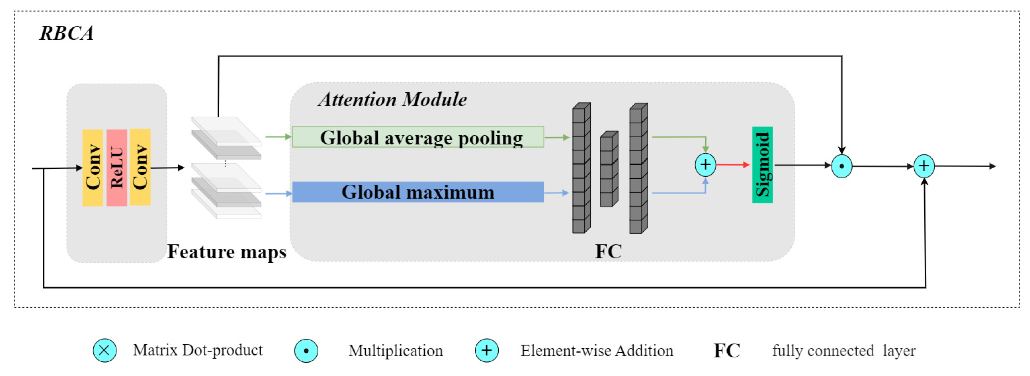
As Figure 4 details, the input features undergo a transformation through two convolutional layers with intermediate ReLU activation to extract multimodal information in preparation for the subsequent attention computation. To achieve comprehensive channel characterisation, a dual-pooling strategy is employed. Global Average Pooling (GAP) and Global Max Pooling (GMP) operate in parallel to condense spatial information into channel descriptors. While GAP captures the overall response of each channel, GMP emphasises salient features, jointly mitigating the bias of single pooling. These descriptors are then processed by a two-layer shared MLP that models inter-channel dependencies. Subsequently, the vectors derived from GAP and GMP are fused via element-wise summation and normalised through sigmoid activation to yield channel-specific weights in the range (0, 1). Finally, these weights are used to recalibrate the convolutional features via channel-wise multiplication, thereby enhancing the critical channels and suppressing the less important ones. To complete residual learning, the original inputs are added to the weighted features to produce the RBCA output.
Thus, the complete operation of an RBCA module can be summarised as:
F b ( d ) = F b 1 ( d ) + W b 1 ( d ) × T ( F b 1 ( d ) )
In this equation, F b 1 ( d ) is the input feature to the b-th RBCA module and F b ( d ) is its output, which also serves as the input to the ( b + 1 ) -th module if multiple RBCAs are stacked. T ( F b 1 ( d ) ) represents the aforementioned feature transformation process Conv ( ReLU ( Conv ( F b 1 ( d ) ) ) ) and W b 1 ( d ) are the channel attention weights. These weights are generated by processing the input F b 1 ( d ) through two parallel paths: GAP and GMP. The resulting feature vectors are then fused via element-wise summation and passed through a shared MLP, followed by a Sigmoid activation function. Conv and ReLU denote the convolution operation and ReLU activation function, respectively.
Following spectral refinement by the RBCA module, the enhanced feature sequence is processed through stacked SABs. These SABs have the same architecture as the SAB in the panchromatic encoder. Since the spectral characteristics have already been optimised, the SAB focuses exclusively on modelling long-range spatial dependencies and global context. This captures the complex inter-location associations within the MS imagery, providing insight into the overall structural patterns.
Ultimately, the encoder outputs F MS R H × W × d i m , which is a spatially preserved spectral representation combining globally modelled spatial information with maximally retained spectral fidelity thanks to the early intervention of the RBCA module. This balanced representation allows the HSSTN to perform high-fidelity pansharpening.

3.3. Hierarchical Fusion Network

The dual-stream feature extractor initially provides modality-specific, optimised panchromatic ( F PAN ) and multispectral ( F MS ) features. To combine the spatial details and structure of F PAN with the spectral fidelity and context of F MS , we designed a hierarchical fusion network. This network decomposes crossmodal fusion into three progressive stages: shallow-level detail injection, mid-level structural aggregation, and deep-level global refinement. Each stage uses task-specific mechanisms to progressively enhance spatial information while maintaining spectral characteristics.

3.3.1. Shallow Fusion

The shallow fusion stage improves the interaction between bidirectional details using local attention mechanisms to supplement and align fine-grained features such as high-frequency textures and edges. This stage processes F PAN R H × W × d i m and F MS R H × W × d i m from their respective encoders. As pixel-level alignment and high-frequency detail injection are the primary initial fusion tasks, local attention confinement prevents the premature mixing of global information. This optimises computational efficiency while preserving spectral integrity.
Inspired by the work of [53], the shallow fusion stage of the HSSTN implements bidirectional interaction between MS and PAN features using a CAB. Its basic structure is similar to that of an SAB, but its core attention mechanism is cross-attention, as shown in Figure 3b. Bidirectional interaction is implemented via CABs, where features from one modality generate the query (Q), and features from the other modality provide the key (K) and value (V). This mechanism enables the selective absorption of complementary information within localised windows, prioritising texture alignment and edge enhancement over global feature mixing.
CAB processing yields enhanced features: F MS R H × W × d i m , which incorporates PAN-derived spatial details, and F PAN R H × W × d i m , which is enriched with MS spectral contexts. These mutually augmented representations provide correlated inputs for subsequent structural aggregation.

3.3.2. Mid-Level Fusion

The mid-level fusion stage is based on the bidirectionally enhanced features, F MS and F PAN , derived from the shallow fusion stage. The focus here is on constructing and enhancing primary structural information. This stage integrates multi-scale structural representations from both modalities to address potential discrepancies in the abstraction level.
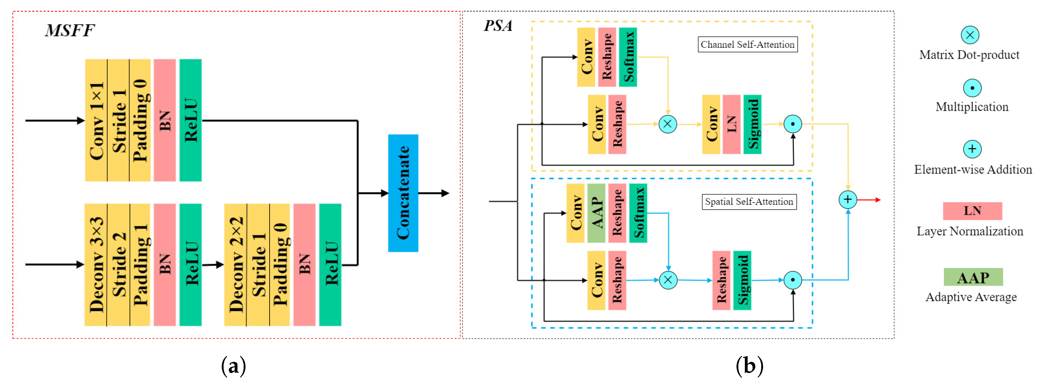
The Multi-Scale Feature Fusion (MSFF) module processes these inputs via parallel transformation paths, performing independent feature re-abstraction prior to channel-wise concatenation [54]. As illustrated in Figure 5a, this architecture uses modality-specific structural information to generate a comprehensive fused feature F MidFused R H × W × d i m . This amalgamated representation combines enhanced spatial details with structural semantics, providing optimised inputs for subsequent refinement stages.
The rationale for this concatenate-first strategy is to create a unified, crossmodal feature space before the final refinement stage. By combining the spatially enhanced MS features and spectrally enriched PAN features into a single, richer tensor, we enable the subsequent PSA module to learn complex, non-linear dependencies between the spectral and spatial domains simultaneously. This deep fusion approach is more powerful than applying separate attention mechanisms to each branch, as it allows the model to explicitly model how specific spatial structures should influence spectral characteristics, and vice versa, leading to a more coherent and high-fidelity fusion.

3.3.3. Deep Fusion

The deep fusion stage is the final phase of the hierarchical fusion process. Its purpose is to refine the global context and optimise the quality of the deeply fused features. This stage ensures large-scale structural coherence and visual consistency, as well as the balanced integration of spectral and structural information. The architecture incorporates parallel channel and spatial self-attention pathways via a Pyramid Squeeze Attention (PSA) module [55], as illustrated in Figure 5b. The channel self-attention branch recalibrates the weights of the feature channels to prioritise significant spectro-spatial components. Meanwhile, the spatial self-attention branch captures long-range dependencies in order to optimise global structures and resolve local inconsistencies.
Integration of these dual attention branches produces the final deep-fused feature F DeepFused R H × W × d i m . This representation embodies the final output of the hierarchical fusion network, being optimised to preserve detail and structural integrity while ensuring global consistency and retaining spectral fidelity. The refined features then feed directly into the reconstruction head for image generation. The HSSTN’s fusion network systematically achieves complex crossmodal integration through progressive, hierarchical processing involving detail injection, structural aggregation, and global refinement. This structured approach establishes the foundation for high-fidelity pansharpened outputs.

3.4. Image Reconstruction Head

The features F DeepFused , which have undergone extensive optimisation by a hierarchical fusion network, contain rich, spectrally preserved and spatially enhanced crossmodal information. In order to transform these features into final high-resolution panchromatic sharpened images, a novel co-optimised loss function was designed during the image reconstruction process. This function ensured that the reconstruction results achieved high fidelity in all three dimensions: pixel, structural, and spectral.

3.4.1. Image Reconstruction Architecture

The architecture of the image reconstruction head adapts a mature image restoration framework from PanFormer [26]. This module upsamples the deep fused features F DeepFused R H × W × d i m to match the spatial resolution of the input panchromatic image ( 4 H × 4 W ) while concurrently adjusting the channel depth to the C-bands of the original multispectral image. This is achieved using a sequence of lightweight convolutions and pixel-shuffling operations defined as I PS = ReconstructionHead ( F DeepFused ) =   Conv 3 × 3 4 × d i m Pixel - Shuffle ( × 2 ) Conv 3 × 3 4 × d i m Pixel - Shuffle ( × 2 ) Conv 3 × 3 d i m Conv 3 × 3 C , which simultaneously recovers fine details and enhances sharpness during the feature-to-image conversion process.

3.4.2. Synergistic Optimisation Loss Function

It is evident that conventional pansharpening methodologies frequently entail the utilisation of L1 or L2 losses for the purpose of model optimisation. While these can ensure pixel-level similarity, they tend to overlook the precise preservation of structural information and spectral fidelity, often leading to blurring or spectral distortion. The present study draws inspiration from the concept of synergistic optimisation as outlined in the extant literature [56,57]. In this research, a novel multi-objective synergistic optimisation loss function, designated as L HSSTN , is proposed. The composite loss function has been developed with the intention of constraining the network’s learning from multiple dimensions simultaneously, with a view to comprehensively enhancing the quality of the fused image. The model under consideration is composed of three weighted components, which are designed to function collectively. The components in question are as follows: a pixel-level fidelity loss, denoted by L pixel ; a structural similarity loss, denoted by L structure ; and a spectral fidelity loss, denoted by L spectral . It is defined as follows:
L HSSTN = λ 1 L pixel + λ 2 L structure + λ 3 L spectral
where λ 1 ,   λ 2 , and λ 3 are weighting hyperparameters used to balance the contributions of the different loss terms.
For pixel-level accuracy, we employ the L1 loss to measure the difference between the generated sharpened image I PS and the ground truth high-resolution multispectral image I GT . Compared to the L2 loss, the L1 loss offers greater robustness to outliers and encourages the generation of sharper edges.
L pixel = I PS I GT 1
In order to optimise the preservation of the local structure and textural details of the image, the Structural Similarity Index Measurement (SSIM) is utilised as a loss term [58]. SSIM is a metric that is employed to assess the similarity between images from three distinct perspectives: luminance, contrast, and structure. This approach is founded on the premise that it reflects human visual perception more effectively than purely pixel-based losses.
L structure = 1 SSIM ( I PS , I GT )
To address the critical challenge of spectral distortion in pansharpening, we innovatively introduce the Error Relative to the Global Average Spectral (ERGAS) [59] index as a direct constraint for spectral preservation. ERGAS globally assesses the spectral differences across all bands of the multispectral image. Incorporating it into the loss function explicitly compels the network to strictly preserve the original spectral characteristics during the optimisation process.
L spectral = ERGAS ( I PS , I GT )
By synergistically integrating these pixel, structural, and spectral constraints, our co-optimised loss function guides the HSSTN model during end-to-end training. Consequently, it generates pansharpened images that exhibit not only high visual clarity and rich detail but also superior spectral fidelity, effectively overcoming the intrinsic limitations of traditional single-objective optimisation approaches.

4. Experiments and Results

This section evaluates the proposed HSSTN network. We begin by outlining the experimental setup, including the datasets, evaluation metrics and baselines, and implementation details. The model’s performance is then assessed through quantitative and qualitative comparisons on Gaofen-2, QuickBird, and WorldView-3 imagery. An ablation study concludes the section, analyzing the importance of key architectural components.

4.1. Datasets

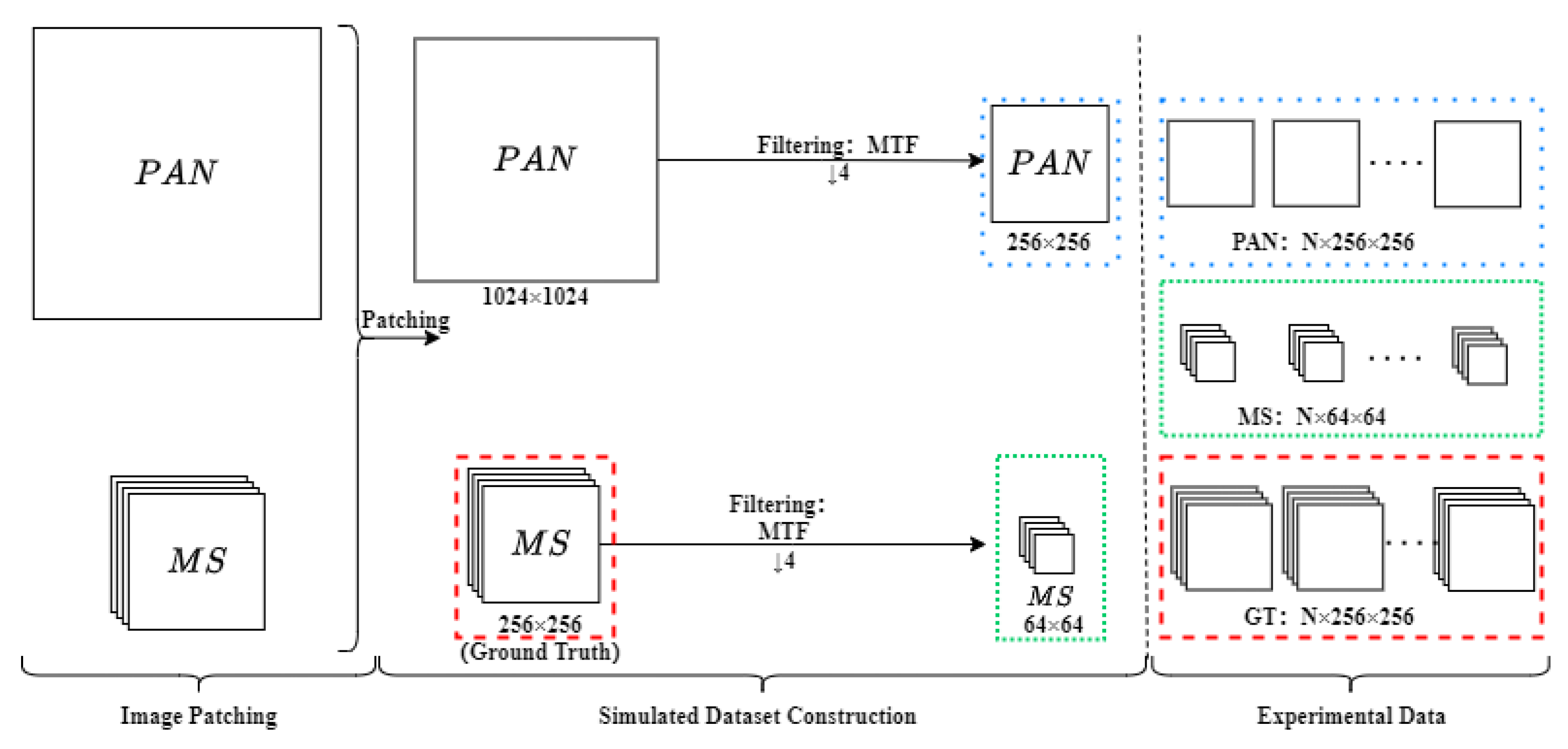
Since ground truth (GT) images are unavailable for real-world pansharpening, we generate a synthetic dataset following the widely adopted Wald’s protocol. In this framework, an original multispectral (MS) image is spatially degraded to create the low-resolution MS input for the network. The original MS image serves as the ground truth, while its downsampled version is used as the MS input for training. This workflow is illustrated in Figure 6.
In this paper, three types of remote sensing data—QuickBird, GaoFen-2, and WorldView-3—are used for experiments. Table 1 summarises the details and technical information of the satellite imagery. We prepare the datasets by cropping the original acquired MS and Pan images with sizes of 256 × 256 pixels (resampled by a factor of 4) and 256 × 256 pixels, respectively. From each acquired satellite image, we use the area of interest regions with important features of the area.
  • QuickBird: The QuickBird dataset is from Vidan Sabha, Jaipur Rajasthan, India, dated 18 October 2013, with a resolution of 2.8 m in MS and 0.7 m in PAN. The PAN image is 256 × 256 pixels and the MS image is 64 × 64 pixels.
  • GaoFen-2: This dataset represents an urban area of Guangzhou, China. The GaoFen-2 dataset is dated August 2014. The Gaofen-2 satellite provides a PAN image with a spatial resolution of 0.8 m and a 4-band MS image with a resolution of 3.2 m. The sensor captures data with a 10-bit depth, covering Blue, Green, Red, and NIR spectral bands.
  • WorldView-3: This dataset represents an urban area of Adelaide, South Australia. The WorldView-3 dataset is dated 27 November 2014 with resolution of 1.2 m 8-band BundleMS and 0.3 m in PAN. The pansharpened multispectral image that we would like to estimate has 256 × 256 × 8 pixels. The dataset has been acquired by the WorldView-3 sensor, which provides a high-resolution PAN channel and eight MS bands.

4.2. Evaluation Indicators and Comparison Methods

To quantitatively assess fusion performance, six widely adopted evaluation metrics were employed across all three datasets. These metrics include the following: Spatial Correlation Coefficient (SCC) [62], Error Relative to the Global Average Spectral (ERGAS) [59], the extended version of Q (Q4/Q8) [63], Structural Similarity Index Measurement (SSIM) [58], Hybrid QNR (HQNR) [64], Spectral Angle Mapper (SAM) [65], spectral distortion ( D λ ), and spatial distortion ( D s ). Among these metrics, higher values of SCC, Q4, SSIM, and HQNR indicate superior fusion quality, while lower values of ERGAS, D λ , D s , and SAM represent better performance.
Furthermore, to demonstrate the effectiveness of the proposed method, nine state-of-the-art pansharpening algorithms were selected for comparative analysis: Brovey [66], HPF [67], PNN [18], PanNet [34], PSGAN [37], PGMAN [48], LDP-Net [45], PanFormer [26], FAFormer [68], PLRDiff [50], and Pan-Mamba [40]. These benchmark methods encompass both unsupervised approaches (Brovey, HPF, PGMAN, LDP-Net, and PLRDiff) and supervised deep learning techniques (PNN, PanNet, PSGAN, PanFormer, FAFormer, and Pan-Mamba), providing a comprehensive evaluation framework across different methodological paradigms.

4.3. Experimental Details

All experiments were implemented in Python 3.8 using the PyTorch framework and were run on a server equipped with dual NVIDIA GeForce RTX 3070 GPUs, 94 GB of RAM, and an Ubuntu 20.04 operating system. For model training across all datasets, we consistently used the Adam optimiser with betas of (0.9, 0.999) and an initial learning rate of 5 × 10 5 . A StepLR scheduler was applied to reduce the learning rate by a factor of 0.9 every 5000 iterations. We trained the model for 200,000 iterations with a batch size of 1. The weighting hyperparameters for our synergistic loss function were uniformly set to λ 1 = 0.5 , λ 2 = 0.1 , and λ 3 = 0.02 .

4.4. Experimental Results

To validate the effectiveness of the proposed method, comprehensive experiments were conducted on three satellite datasets using both full-scale and reduced-scale versions. The evaluation encompasses visual comparisons and quantitative analysis across QuickBird, GaoFen-2, and WorldView-3 datasets. All test samples were carefully selected to ensure complete independence from training data, with no spatial overlap, thereby guaranteeing unbiased and reliable evaluation results.

4.4.1. GaoFen-2 Dataset

To undertake an objective evaluation of the proposed algorithm’s performance, the experimental results on the dataset are compiled in Table 2. In the ensuing quantitative results, the optimal value for each metric is emphasised in bold, while the second-best is underlined. This formatting facilitates a clearer identification of the methods that achieve optimal and near-optimal performance. As demonstrated in the table, the proposed method demonstrates optimal performance in terms of the SCC, ERGAS, and Q4 metrics. Furthermore, it achieves the second-best results for the SSIM, HQNR, SAM, D λ , and D s metrics, with values that closely approach the leading scores.
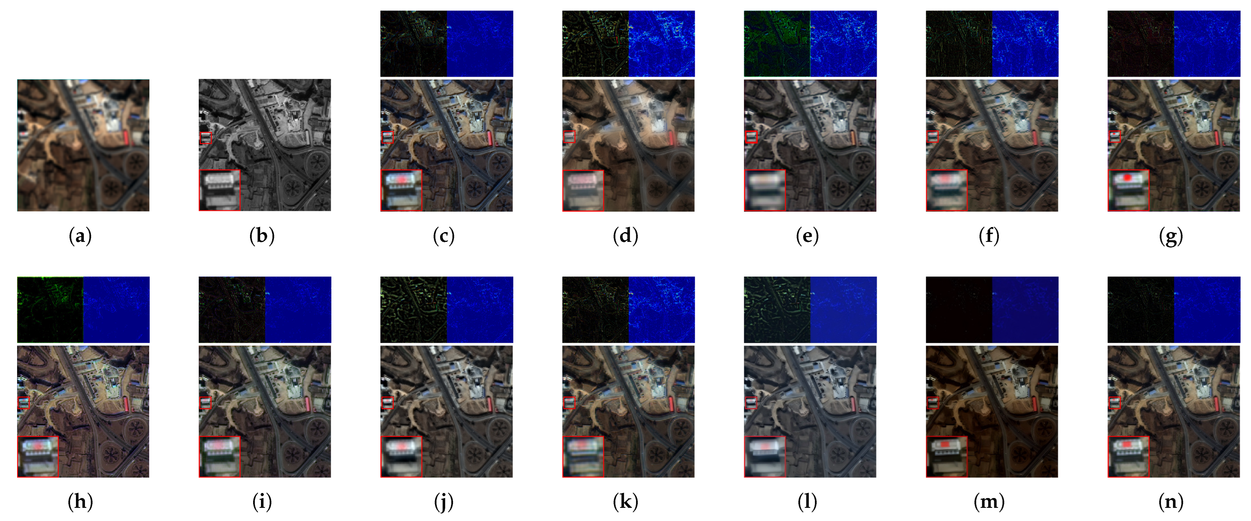
To comprehensively validate the performance of the proposed algorithm, a comparative analysis was conducted against other state-of-the-art methods using a representative pair of images under both reduced-resolution and full-resolution experimental setups. The results of this analysis are illustrated in Figure 7 and Figure 8, respectively. In both figures, the MS and PAN images are presented in (a) and (b). The MS image is distinguished by its rich spectral information, yet it is visually indistinct. Conversely, the PAN image offers an abundance of spatial detail, albeit in greyscale. In order to facilitate a clearer observation of the subtle distinctions among the different pansharpening methods, the resulting images have been highlighted with red boxes in several areas. The larger red box is a magnified version of the corresponding smaller box. By enlarging these specific regions, the differences between the fusion algorithms in terms of detail preservation and spectral fidelity can be more distinctly examined.
In the full-scale setting, as illustrated in Figure 7, unsupervised methods such as the Brovey technique exhibit significant spectral colour distortion, with rooftops appearing in greyish-pink hues in the fused results. Supervised methods, such as PanNet, have been observed to demonstrate a clear loss of edge details in magnified images, resulting in the appearance of blurring artefacts. In contrast, the proposed method not only recovers building edges with reasonable fidelity but also achieves superior performance in preserving blue and red colour characteristics.
In the more stringent reduced-scale experiment (as shown in Figure 8), the performance disparities among the algorithms become more pronounced. The image fused by HPF exhibits significant colour deviation, indicating poor spectral fidelity. Methods such as PGMAN and LDP-Net produce images with an overall dark-red bias, which is likely attributable to spectral mixing artefacts. Regarding edge details, although these two methods yield sharp images, they suffer from over-sharpening phenomena, resulting in unnatural ”halo“ effects around object edges. Overall, these unsupervised methods fail to effectively balance the preservation of spectral and spatial information under reduced-scale conditions, leading to suboptimal performance. Among the supervised methods, Pan-Mamba demonstrates strong competitive performance, as the colours and edges of the sports field in the magnified view are well preserved. In comparison, however, the proposed method achieves superior spectral fidelity, delivering more realistic colour restoration for areas such as the running track and the lawn. Furthermore, our method also exhibits superior performance in the enhancement of texture details, rendering the texture of the grass more clearly and naturally.
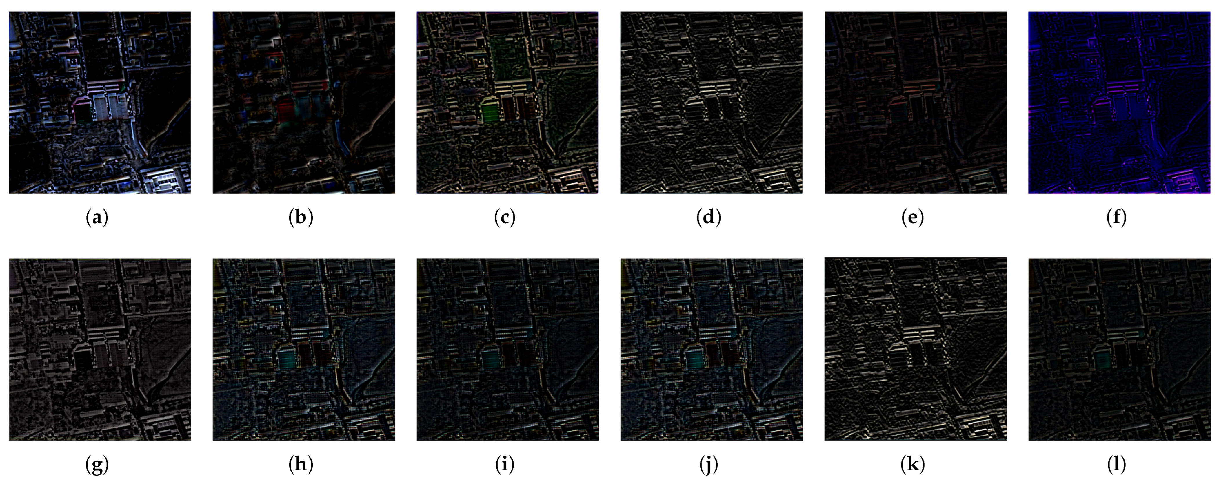
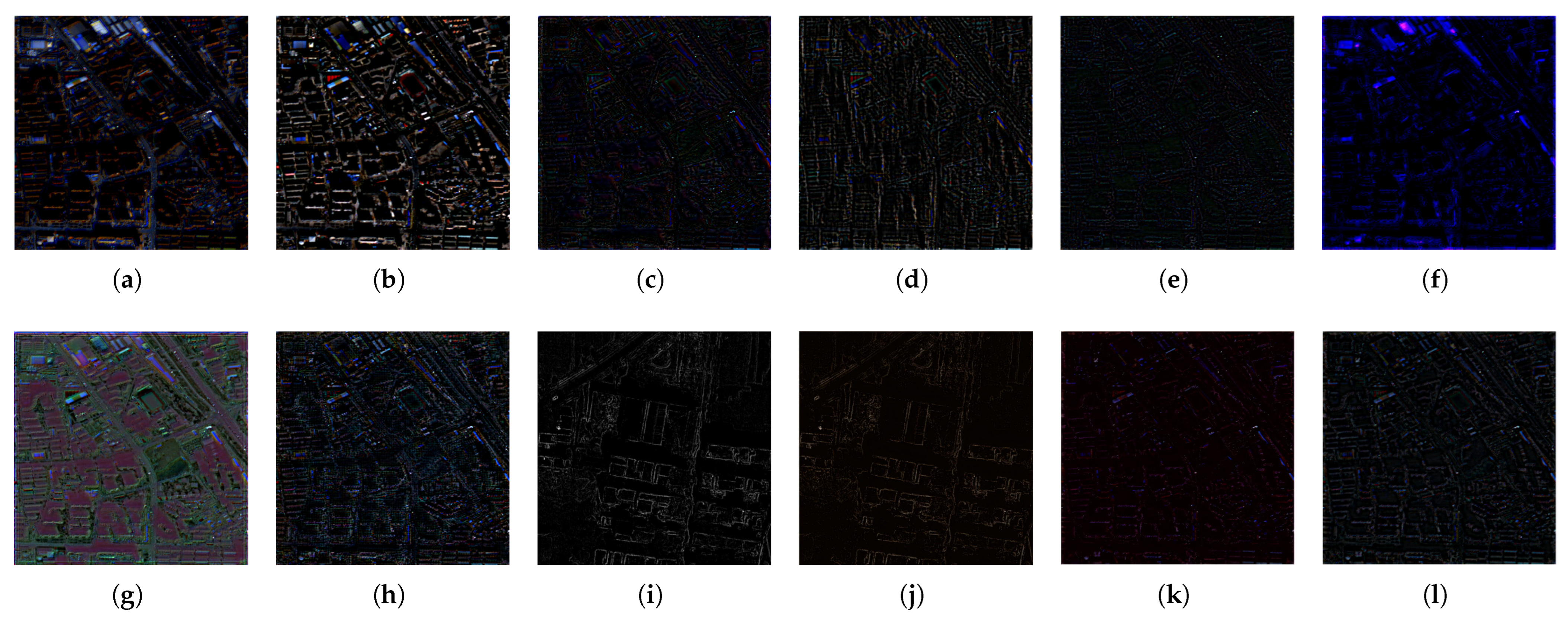
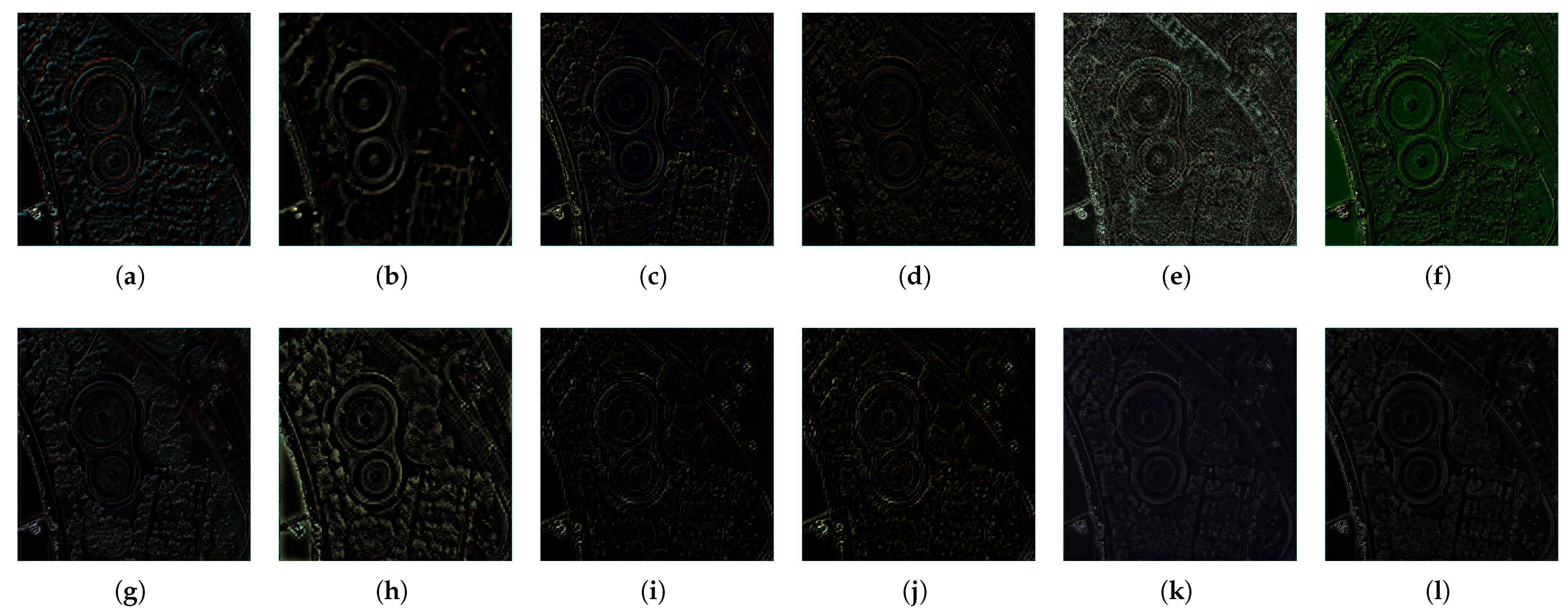
To more directly quantify and visualise the spectral preservation capabilities of the different algorithms, this study further introduces a residual analysis. We computed the four-channel spectral residuals between the fusion result of each model and the reference MS image (using the simulated ground truth for the reduced-scale experiment and the original MS image for the full-scale experiment). The resulting spectral residual maps are presented in Figure 9 and Figure 10. In these visualisations, darker colours signify smaller spectral deviations, meaning the spectral distribution of the fusion image is closer to that of the reference image. Under the full-scale setting (Figure 9), methods like PGMAN and PanFormer show varying degrees of spectral information loss, manifested as brighter areas in their respective maps. In the reduced-scale environment (Figure 10), the spectral deviations of HPF, Brovey, and LDP-Net are particularly severe, as their residual maps are predominantly bright. Even a strong performer like Pan-Mamba (Figure 10k) displays faint yet visible residual structures, indicating small but measurable inaccuracies. In contrast, as shown in Figure 9l and Figure 10l, the residual maps of our method exhibit the darkest tones overall in both experimental scales. This visually demonstrates that the spectral difference between our fusion result and the reference image is minimal, confirming its leading spectral preservation capability among all compared algorithms.
In summary, the proposed HSSTN method demonstrates exceptional pansharpening performance on the GaoFen-2 dataset, as shown by the quantitative evaluation, qualitative visual comparison, and spectral residual analysis. In terms of both the fidelity of spatial structures and the preservation of spectral information, the images it generates most closely approximate the reference standard.

4.4.2. QuickBird Dataset

To validate the generalisation capability of our algorithm, we conducted a comprehensive quantitative evaluation on the QuickBird dataset, with the results detailed in Table 3. An analysis of this table reveals that the proposed HSSTN method achieves the optimal (bolded) results in four key metrics: SCC, Q4, D s , and the HQNR index. Although it did not rank first in ERGAS, SSIM, and SAM, its scores are highly competitive and minimally distanced from the best values, demonstrating the robustness and balance of its performance. Overall, the quantitative results from the QuickBird dataset further confirm that the HSSTN method is not overfitted to a specific dataset but is a generalisable and highly effective pansharpening solution.
The advantages of our method are also visually evident in the full-scale comparison on the QuickBird dataset (as shown in Figure 11). Observing the magnified regions (yellow boxes), traditional methods like Brovey (c) and HPF (d) exhibit noticeable spectral distortion, with the blue rooftop appearing in unnatural purple or faded tones. Some deep-learning-based methods, such as PNN (e) and PanNet (g), while improved in colour, are deficient in detail depiction, resulting in slightly blurred edges and textures on the rooftop. In contrast, the image generated by our method (n) is visually superior: the blue of the rooftop is pure and uniform, the edges are sharp and well-defined, and the fine surface textures are faithfully restored. Even when compared to high-performing algorithms like Pan-Mamba (m), our method shows a slight edge in colour saturation and the naturalness of details, leading to a more visually pleasing overall image.
The reduced-scale experiment (Figure 12) provides a basis for evaluating the algorithm’s robustness under more challenging conditions. In this setting, the results from Brovey (c) and HPF (d) are once again compromised by severe spectral distortion, reducing their utility. Other methods show an imbalance between detail and spectral preservation, leading to either blurring or artefacts. The result from our method, shown in (n), appears both sharp and natural within the magnified region (red box). The outlines of buildings, the lines of roads, and the sparse vegetation are all clear. The image not only maintains high spatial sharpness but also features colours that are highly consistent with the original multispectral image, without oversaturation or colour shifts. This demonstrates that even with greater information loss, the HSSTN can still accurately fuse spectral and spatial information to produce high-quality pansharpened images.
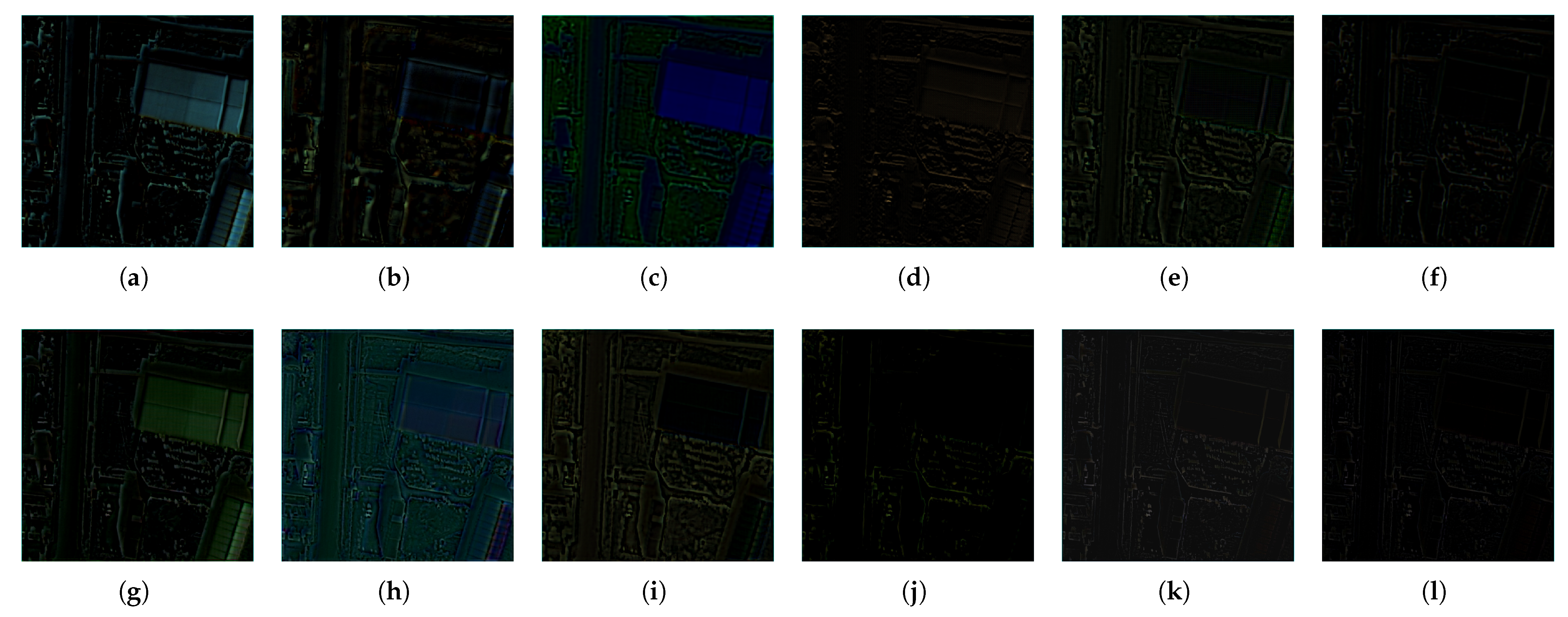
In the full-scale residual maps (Figure 13), the maps for Brovey (a) and HPF (b) are bright, visually exposing their severe loss of spectral information. Most other methods also show faint, bright “ghosts” corresponding to object contours, indicating spectral deviations at edge regions. Among all methods, the residual map for our approach (l) is the darkest and contains almost no visible structural information, providing strong proof that the spectral difference between its fusion result and the reference image is minimal. In the reduced-scale experiment (as seen in the residual maps above each subplot in Figure 12), the residual map corresponding to our method (n) is the darkest with the lowest brightness. This result is perfectly consistent with the quantitative metrics and qualitative appearance, once again confirming the outstanding performance of the HSSTN in spectral preservation.
In conclusion, the quantitative, qualitative, and residual analyses conducted on the QuickBird dataset validate the effectiveness and generalisation capability of the proposed HSSTN method. Across both objective performance metrics and subjective visual quality, HSSTN demonstrates state-of-the-art or highly competitive performance. The experimental results clearly show that the method can successfully inject high-resolution spatial information into multispectral images while maximally suppressing spectral distortion and artefacts. Its performance remains stable across different sensors and scenes, highlighting its significant potential as an advanced pansharpening technique.

4.4.3. WorldView-3 Dataset

We conducted rigorous quantitative tests on the WorldView-3 dataset, which contains eight multispectral bands. The results are presented in Table 4. Faced with the challenges posed by double the number of spectral bands, the proposed HSSTN method demonstrates a more significant advantage, achieving optimal (bolded) results in five key metrics: SCC, ERGAS, Q8, SAM, and D λ . Notably, the lowest ERGAS and SAM values are the most direct quantitative measures of spectral fidelity. Winning in these two core spectral metrics proves the method’s exceptional ability to suppress spectral distortion in high-dimensional data. Simultaneously, the highest SCC score ensures optimal spatial detail injection, while the leading Q8 value indicates the best performance in preserving the complex spectral relationships across all eight bands. Furthermore, the method also achieves competitive second-best results in SSIM and HQNR, with values very close to the optimal scores.
In the full-scale visual comparison on the WorldView-3 dataset (Figure 14), the magnified region (red box) shows a plaza with a concentric circle structure. The result from a traditional method like HPF (d) is severely blurred, making it impossible to discern the fine structures of the plaza. While some deep learning methods offer improved clarity, they suffer from varying degrees of spectral distortion or artefacts; for example, the colours of vegetation and tiles appear unnatural in some results. In contrast, the fusion result from our method (n) achieves top-tier performance in both clarity and fidelity. Every concentric circle edge in the plaza is sharp and clear, the grid texture of the tiles is distinct, and the colours of the surrounding vegetation and buildings are rendered realistically and naturally.
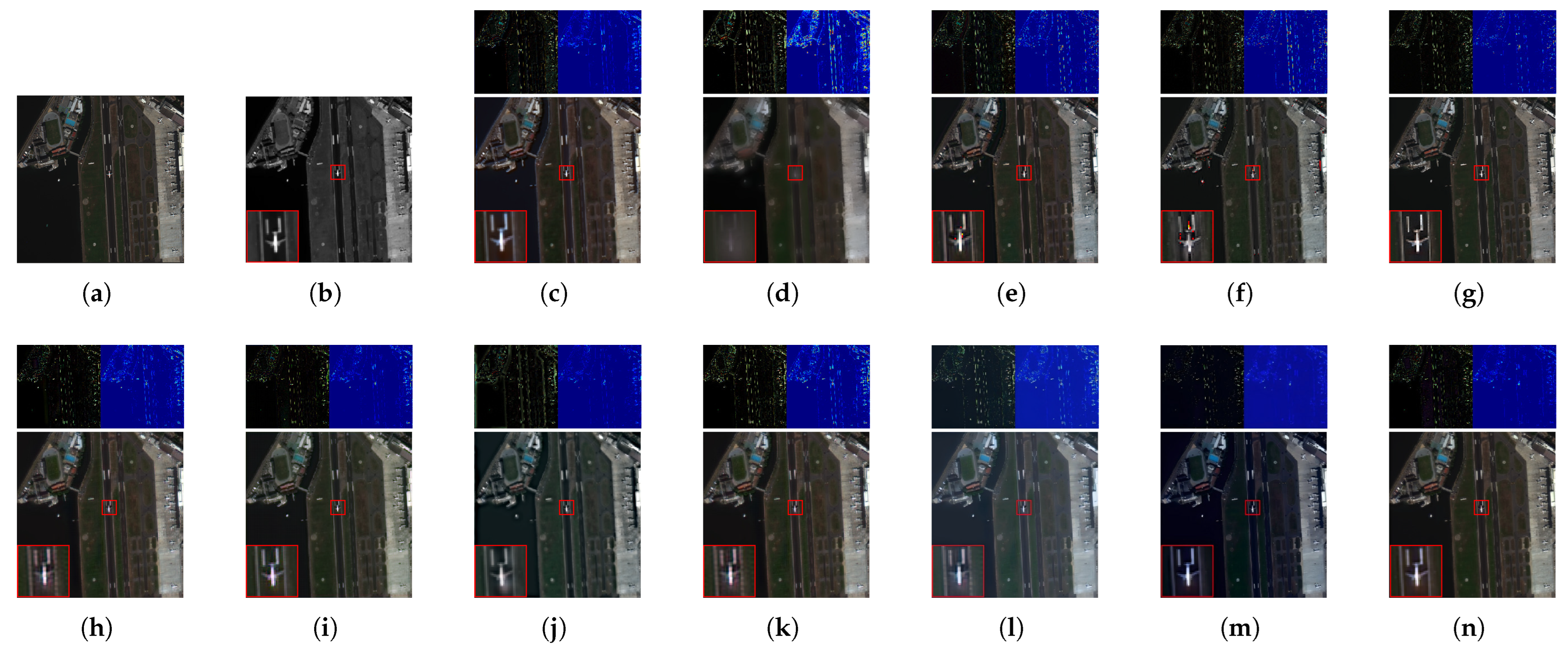
The reduced-scale experiment (Figure 15) incorporates diverse elements, including an aeroplane on an apron, water bodies, and vegetation. From the magnified region (red box), it is evident that in many competing methods’ results, the aeroplane’s outline is blurry or even merges with the background, making it difficult to identify. For instance, in the results of Brovey (c) and HPF (d), not only is the spectral distortion severe, but the aeroplane target is also significantly degraded by artefacts. Our method (n), however, successfully reconstructs the sharp outline of this small target, with details such as the fuselage and wings being recognisable. At the same time, the apron markings, the colour of the water, and the spectral information of surrounding features are well preserved, leading to a clear and natural overall image. This indicates that HSSTN has a significant advantage in preserving small targets and maintaining comprehensive information in complex scenes.
The spectral residual analysis provides critical visual evidence for evaluating the 8-band data. The full-scale residual maps (Figure 16) for methods like Brovey (a), HPF (b), and PGMAN (f) display very bright colours and clear object structures, indicating a large spectral discrepancy between their fused results and the original multispectral image. In contrast, the residual map corresponding to our method (l) is the darkest and most uniform among all competitors, with almost no visible residual structures. In the reduced-scale experiment (as seen in the residual maps above each subplot in Figure 15), the residual map for our method (n) is again the darkest, proving that the HSSTN can achieve optimal spectral fidelity even at a reduced resolution.
In conclusion, through systematic experiments on the 8-band WorldView-3 dataset, the proposed HSSTN method has demonstrated its formidable capability. Whether in quantitative metrics or qualitative visual assessments of complex features and small objects, the HSSTN consistently outperforms or matches existing mainstream methods. It has achieved a significant breakthrough in addressing the core challenge of spectral fidelity thanks to its innovative network design.

4.4.4. Efficiency Analysis

To evaluate the practical applicability of the proposed method, we compare its complexity and efficiency with other deep-learning-based approaches. The number of trainable parameters and Floating Point Operations (FLOPs) and the average inference time were measured. FLOPs and inference time were calculated on an input image pair with a PAN size of 400 × 400 and an MS size of 100 × 100. All inference times were benchmarked on a single NVIDIA GeForce RTX 3070 GPU. The results are summarised in Table 5.
As is evident from the data in Table 5, our proposed HSSTN model achieves a balance between model complexity and computational efficiency. In terms of parameter count, our model is one of the most lightweight among all the compared methods, with only 0.38 M parameters. This size is substantially lower than models such as PanFormer (1.62 M) and PSGAN (2.44 M), and it is three orders of magnitude smaller than the computationally expensive PLRDiff model (391.05 M). Regarding computational load (FLOPs), our method’s 6.10 G is also a low level, significantly less than PanFormer (61.01 G), PSGAN (33.79 G), and Pan-Mamba (16.02 G). In terms of inference speed, our model has an average inference time of 0.13 s for a single image pair. While slightly slower than some models with minimalist architectures, this speed is highly competitive compared to other state-of-the-art methods with similar performance, and it is considerably faster than Transformer-based architectures like FAFormer (0.34 s) and PanFormer (0.40 s).

4.5. Ablation Study

To validate the effectiveness and necessity of the core components within our proposed HSSTN model, we conducted a series of comprehensive ablation studies on both the QuickBird and GaoFen-2 datasets. We focused on evaluating three key modules: the RBCA, the MSFF module, and the PSA module. The experiments are divided into two parts, “module removal” and “module replacement”, to thoroughly justify the rationality of our architectural design. All experimental results are recorded in Table 6.
We sequentially removed the RBCA, MSFF, and PSA modules from the complete HSSTN model to observe the performance changes. As shown in the “Removal Ablation Studies” section of Table 6, removing the MSFF module (w/o MSFF) caused the most significant drop in performance, particularly for the ERGAS metric, where the error increased from 1.5921 to 1.7245 on the QuickBird dataset and from 0.8789 to 0.9608 on the GaoFen-2 dataset. Similarly, removing the RBCA module (w/o RBCA) also resulted in a noticeable performance decline, confirming its core function in extracting deep, discriminative features and focusing on key channel information. Although the performance drop from removing the PSA module (w/o PSA) was slightly smaller, it was still clearly discernible, validating its effectiveness in capturing and enhancing key spatial structures.
To further demonstrate the superiority of our module designs, we conducted a series of module replacement studies. We replaced the RBCA with a standard 3 × 3 convolution, the MSFF with a simple “1 × 1 convolution + concatenation” operation, and the PSA with a generic spatial attention mechanism, as shown in the “Replacement Ablation Studies” section of Table 6. For instance, using a simple concatenation operation to replace the MSFF module could not achieve the same level of multi-scale information aggregation, leading to a significant decline in performance. Furthermore, replacing PSA with a generic spatial attention mechanism also led to lower performance, suggesting that our proposed pyramid structure is more effective at capturing the multi-scale spatial context required for the pansharpening task.

5. Discussion

The comprehensive experimental results presented in this study position our proposed HSSTN as a pansharpening method, distinguished by its high accuracy and broad generalisation capabilities. the model’s consistent performance across three distinct datasets, from the 4-band sensors of GaoFen-2 and QuickBird to the more spectrally complex 8-band WorldView-3 data. This demonstrates that the HSSTN’s architectural design is not narrowly tuned to a specific data type but is fundamentally effective at navigating the core challenges of the pansharpening task. The success on the WorldView-3 dataset is particularly noteworthy, as increasing spectral dimensionality often exacerbates spectral distortion in many algorithms. The HSSTN’s superior performance in this challenging scenario, evidenced by its leading scores in key spectral metrics like ERGAS and SAM, underscores the efficacy of its asymmetric dual-stream architecture, which respects and processes the distinct characteristics of multispectral and panchromatic information.
Beyond accuracy, a significant conclusion of this work is that the HSSTN strikes an exceptional balance between performance and computational efficiency, a critical factor for practical applications. While many recent high-performing models achieve accuracy at the cost of enormous computational overhead (e.g., PLRDiff with over 390 M parameters), our model delivers its state-of-the-art results with a remarkably lightweight footprint of only 0.38 M parameters and 6.10 G FLOPs. This efficiency is not an accident but a direct result of its targeted design. The ablation studies provide definitive evidence for this, revealing that each core component (RBCA, MSFF, PSA) is not only necessary but also superior to simpler or generic alternatives. This confirms that the HSSTN’s performance stems from the intelligent and synergistic combination of efficient, purpose-built modules, rather than from brute-force computation. This blend of high accuracy, strong generalisation, and low computational cost makes the HSSTN a highly practical and promising solution for real-world remote sensing applications where both quality and efficiency are paramount.

6. Conclusions

In this paper, we propose a novel pansharpening network, the HSSTN, to address the core challenge of balancing spectral fidelity and spatial detail enhancement. Through its asymmetric dual-stream encoder and hierarchical fusion network, the HSSTN achieves exceptional performance. Comprehensive experiments across diverse datasets, including GaoFen-2, QuickBird, and the more challenging 8-band WorldView-3, demonstrate that our method not only makes a breakthrough in accuracy and visual quality but, crucially, does so with 0.38 M parameters. Ablation studies confirm that this success stems from the efficient and synergistic design of its core modules. HSSTN strikes an outstanding balance between accuracy, efficiency, and generalisation, providing a highly practical and advanced solution for the field of remote sensing image fusion. Looking forward, its core crossmodal fusion concepts could be extended to other remote sensing challenges, including SAR–optical and hyperspectral–multispectral fusion. Finally, exploring self-supervised learning paradigms could reduce the dependency on simulated data, further enhancing the model’s practicality and robustness.

Author Contributions

Conceptualisation, W.K., Y.F., Y.D., and Y.C.; methodology, W.K., H.X., X.L., and Y.C.; software, W.K., Y.D., and H.X.; validation, W.K., Y.F., and Y.D.; formal analysis, W.K., Y.F., Y.D., H.X., X.L., and Y.C.; investigation, W.K., Y.F., Y.D., and Y.C.; resources, W.K., H.X., and Y.C.; data curation, Y.F., Y.D., H.X., and X.L.; writing—original draft preparation, W.K., Y.F., and H.X.; writing—review and editing, Y.F., Y.D., X.L., and Y.C.; supervision, W.K. and Y.C. All authors have read and agreed to the published version of the manuscript.

Funding

This research was supported in part by the National Natural Science Foundation of China (Nos. 72401292 and 62401632), in part by the Hubei Provincial Natural Science Foundation of China (No. 2024AFB484), in part by China Postdoctoral Science Foundation (No. 2024M753661); in part by the Postdoctoral Fellowship Program (Grade C) of China Postdoctoral Science Foundation (No. GZC20233138), and in part by the Joint Open Fund of the Research Platforms of School of Computer Science, China University of Geosciences, Wuhan (No. PTLH2024-B-06).

Institutional Review Board Statement

Not applicable.

Informed Consent Statement

Not applicable.

Data Availability Statement

The data presented in this study is available on request from the corresponding author.

Conflicts of Interest

The authors declare no conflicts of interest.

References

  1. Perretta, M.; Delogu, G.; Funsten, C.; Patriarca, A.; Caputi, E.; Boccia, L. Testing the Impact of Pansharpening Using PRISMA Hyperspectral Data: A Case Study Classifying Urban Trees in Naples, Italy. Remote Sens. 2024, 16, 3730. [Google Scholar]
  2. Wang, N.; Chen, S.; Huang, J.; Frappart, F.; Taghizadeh, R.; Zhang, X.; Wigneron, J.P.; Xue, J.; Xiao, Y.; Peng, J.; et al. Global soil salinity estimation at 10 m using multi-source remote sensing. J. Remote Sens. 2024, 4, 0130. [Google Scholar] [CrossRef]
  3. Zhang, X.; Chen, H.; Zhao, Y.; He, M.; Han, X. Change detection of buildings in remote sensing images using a spatially and contextually aware Siamese network. Expert Syst. Appl. 2025, 276, 127110. [Google Scholar] [CrossRef]
  4. Wang, S.; Zou, X.; Li, K.; Xing, J.; Cao, T.; Tao, P. Towards robust pansharpening: A large-scale high-resolution multi-scene dataset and novel approach. Remote Sens. 2024, 16, 2899. [Google Scholar] [CrossRef]
  5. Deng, L.J.; Vivone, G.; Paoletti, M.E.; Scarpa, G.; He, J.; Zhang, Y.; Chanussot, J.; Plaza, A. Machine learning in pansharpening: A benchmark, from shallow to deep networks. IEEE Geosci. Remote Sens. Mag. 2022, 10, 279–315. [Google Scholar] [CrossRef]
  6. Zini, S.; Barbato, M.P.; Piccoli, F.; Napoletano, P. Deep Learning Hyperspectral Pansharpening on Large-Scale PRISMA Dataset. Remote Sens. 2024, 16, 2079. [Google Scholar]
  7. Ciotola, M.; Guarino, G.; Vivone, G.; Poggi, G.; Chanussot, J.; Plaza, A.; Scarpa, G. Hyperspectral Pansharpening: Critical review, tools, and future perspectives. IEEE Geosci. Remote Sens. Mag. 2025, 13, 311–338. [Google Scholar]
  8. Li, D.; Wang, M.; Guo, H.; Jin, W. On China’s earth observation system: Mission, vision and application. Geo-Spat. Inf. Sci. 2024, 28, 303–321. [Google Scholar]
  9. Cliche, F. Integration of the SPOT panchromatic channel into its multispectral mode for image sharpness enhancement. Photogramm. Eng. Remote Sens. 1985, 51, 311–316. [Google Scholar]
  10. Javan, F.D.; Samadzadegan, F.; Mehravar, S.; Toosi, A.; Khatami, R.; Stein, A. A review of image fusion techniques for pan-sharpening of high-resolution satellite imagery. ISPRS J. Photogramm. Remote Sens. 2021, 171, 101–117. [Google Scholar]
  11. Cui, Y.; Liu, P.; Ma, Y.; Chen, L.; Xu, M.; Guo, X. Pixel-Wise Ensembled Masked Autoencoder for Multispectral Pansharpening. IEEE Trans. Geosci. Remote Sens. 2024, 62, 1–22. [Google Scholar] [CrossRef]
  12. Arienzo, A.; Alparone, L.; Garzelli, A.; Lolli, S. Advantages of nonlinear intensity components for contrast-based multispectral pansharpening. Remote Sens. 2022, 14, 3301. [Google Scholar] [CrossRef]
  13. Gao, H.; Li, S.; Li, J.; Dian, R. Multispectral Image Pan-Sharpening Guided by Component Substitution Model. IEEE Trans. Geosci. Remote Sens. 2023, 61, 5406413. [Google Scholar] [CrossRef]
  14. Xie, G.; Nie, R.; Cao, J.; Li, H.; Li, J. A Deep Multiresolution Representation Framework for Pansharpening. IEEE Trans. Geosci. Remote Sens. 2024, 62, 5517216. [Google Scholar] [CrossRef]
  15. Xu, S.; Zhong, S.; Li, H.; Gong, C. Spectral–Spatial Attention-Guided Multi-Resolution Network for Pansharpening. IEEE J. Sel. Top. Appl. Earth Obs. Remote Sens. 2025, 18, 7559–7571. [Google Scholar] [CrossRef]
  16. Cao, X.; Chen, Y.; Cao, W. Proximal pannet: A model-based deep network for pansharpening. In Proceedings of the AAAI Conference on Artificial Intelligence, Virtual, 22 February–1 March 2022; Volume 36, pp. 176–184. [Google Scholar]
  17. Palsson, F.; Ulfarsson, M.O.; Sveinsson, J.R. Model-based reduced-rank pansharpening. IEEE Geosci. Remote Sens. Lett. 2019, 17, 656–660. [Google Scholar] [CrossRef]
  18. Masi, G.; Cozzolino, D.; Verdoliva, L.; Scarpa, G. Pansharpening by convolutional neural networks. Remote Sens. 2016, 8, 594. [Google Scholar] [CrossRef]
  19. Liu, Q.; Meng, X.; Shao, F.; Li, S. Supervised-unsupervised combined deep convolutional neural networks for high-fidelity pansharpening. Inf. Fusion 2023, 89, 292–304. [Google Scholar] [CrossRef]
  20. Ye, Y.; Wang, T.; Fang, F.; Zhang, G. MSCSCformer: Multiscale Convolutional Sparse Coding-Based Transformer for Pansharpening. IEEE Trans. Geosci. Remote Sens. 2024, 62, 5405112. [Google Scholar] [CrossRef]
  21. Liu, X.; Liu, Q.; Wang, Y. Remote sensing image fusion based on two-stream fusion network. Inf. Fusion 2020, 55, 1–15. [Google Scholar] [CrossRef]
  22. Yang, Y.; Li, M.; Huang, S.; Lu, H.; Tu, W.; Wan, W. Multi-scale spatial-spectral attention guided fusion network for pansharpening. In Proceedings of the 31st ACM International Conference on Multimedia, Ottawa, ON, Canada, 29 October–3 November 2023; pp. 3346–3354. [Google Scholar]
  23. Woo, S.; Park, J.; Lee, J.Y.; Kweon, I.S. CBAM: Convolutional block attention module. In Proceedings of the European Conference on Computer Vision, Munich, Germany, 8–14 September 2018; pp. 3–19. [Google Scholar]
  24. Zhang, K.; Wang, A.; Zhang, F.; Diao, W.; Sun, J.; Bruzzone, L. Spatial and spectral extraction network with adaptive feature fusion for pansharpening. IEEE Trans. Geosci. Remote Sens. 2022, 60, 5410814. [Google Scholar] [CrossRef]
  25. Vaswani, A.; Shazeer, N.; Parmar, N.; Uszkoreit, J.; Jones, L.; Gomez, A.N.; Kaiser, Ł.; Polosukhin, I. Attention is all you need. In Proceedings of the 31st Conference on Neural Information Processing Systems, Long Beach, CA, USA, 4–9 December 2017; Volume 30. [Google Scholar]
  26. Zhou, H.; Liu, Q.; Wang, Y. PanFormer: A transformer based model for pan-sharpening. In Proceedings of the 2022 IEEE International Conference on Multimedia and Expo, Taipei, Taiwan, 18–22 July 2022; pp. 1–6. [Google Scholar]
  27. Bandara, W.G.C.; Patel, V.M. Hypertransformer: A textural and spectral feature fusion transformer for pansharpening. In Proceedings of the IEEE/CVF Conference on Computer Vision and Pattern Recognition, New Orleans, LA, USA, 18–24 June 2022; pp. 1767–1777. [Google Scholar]
  28. Li, Z.; Li, J.; Ren, L.; Chen, Z. Transformer-based dual-branch multiscale fusion network for pan-sharpening remote sensing images. IEEE J. Sel. Top. Appl. Earth Obs. Remote Sens. 2024, 17, 614–632. [Google Scholar] [CrossRef]
  29. Zhang, F.; Zhang, K.; Sun, J.; Wang, J.; Bruzzone, L. DRFormer: Learning Disentangled Representation for Pan-Sharpening via Mutual Information-Based Transformer. IEEE Trans. Geosci. Remote Sens. 2024, 62, 5400115. [Google Scholar] [CrossRef]
  30. Li, S.; Guo, Q.; Li, A. Pan-sharpening based on CNN+ pyramid transformer by using no-reference loss. Remote Sens. 2022, 14, 624. [Google Scholar] [CrossRef]
  31. Meng, Y.; Zhu, H.; Yi, X.; Hou, B.; Wang, S.; Wang, Y.; Chen, K.; Jiao, L. FAFormer: Frequency-Analysis-Based Transformer Focusing on Correlation and Specificity for Pansharpening. IEEE Trans. Geosci. Remote Sens. 2025, 63, 5403413. [Google Scholar] [CrossRef]
  32. Wald, L.; Ranchin, T.; Mangolini, M. Fusion of satellite images of different spatial resolutions: Assessing the quality of resulting images. Photogramm. Eng. Remote Sens. 1997, 63, 691–699. [Google Scholar]
  33. Yuan, Q.; Wei, Y.; Meng, X.; Shen, H.; Zhang, L. A multiscale and multidepth convolutional neural network for remote sensing imagery pan-sharpening. IEEE J. Sel. Top. Appl. Earth Obs. Remote Sens. 2018, 11, 978–989. [Google Scholar] [CrossRef]
  34. Yang, J.; Fu, X.; Hu, Y.; Huang, Y.; Ding, X.; Paisley, J. PanNet: A deep network architecture for pan-sharpening. In Proceedings of the IEEE International Conference on Computer Vision, Venice, Italy, 22–29 October 2017; pp. 5449–5457. [Google Scholar]
  35. Dian, R.; Shan, T.; He, W.; Liu, H. Spectral Super-Resolution via Model-Guided Cross-Fusion Network. IEEE Trans. Neural Netw. Learn. Syst. 2024, 35, 10059–10070. [Google Scholar] [CrossRef] [PubMed]
  36. Dian, R.; Liu, Y.; Li, S. Hyperspectral Image Fusion via a Novel Generalized Tensor Nuclear Norm Regularization. IEEE Trans. Neural Netw. Learn. Syst. 2025, 36, 7437–7448. [Google Scholar] [CrossRef]
  37. Liu, Q.; Zhou, H.; Xu, Q.; Liu, X.; Wang, Y. PSGAN: A generative adversarial network for remote sensing image pan-sharpening. IEEE Trans. Geosci. Remote Sens. 2020, 59, 10227–10242. [Google Scholar] [CrossRef]
  38. Liu, Y.; Dian, R.; Li, S. Low-rank transformer for high-resolution hyperspectral computational imaging. Int. J. Comput. Vis. 2025, 133, 809–824. [Google Scholar] [CrossRef]
  39. Dian, R.; Liu, Y.; Li, S. Spectral Super-Resolution via Deep Low-Rank Tensor Representation. IEEE Trans. Neural Netw. Learn. Syst. 2025, 36, 5140–5150. [Google Scholar] [CrossRef]
  40. He, X.; Cao, K.; Zhang, J.; Yan, K.; Wang, Y.; Li, R.; Xie, C.; Hong, D.; Zhou, M. Pan-mamba: Effective pan-sharpening with state space model. Inf. Fusion 2025, 115, 102779. [Google Scholar] [CrossRef]
  41. Lu, P.; Jiang, X.; Zhang, Y.; Liu, X.; Cai, Z.; Jiang, J.; Plaza, A. Spectral–spatial and superpixelwise unsupervised linear discriminant analysis for feature extraction and classification of hyperspectral images. IEEE Trans. Geosci. Remote Sens. 2023, 61, 5530515. [Google Scholar] [CrossRef]
  42. Ciotola, M.; Guarino, G.; Scarpa, G. An Unsupervised CNN-Based Pansharpening Framework with Spectral-Spatial Fidelity Balance. Remote Sens. 2024, 16, 3014. [Google Scholar] [CrossRef]
  43. Luo, S.; Zhou, S.; Feng, Y.; Xie, J. Pansharpening via unsupervised convolutional neural networks. IEEE J. Sel. Top. Appl. Earth Obs. Remote Sens. 2020, 13, 4295–4310. [Google Scholar] [CrossRef]
  44. Xiong, Z.; Liu, N.; Wang, N.; Sun, Z.; Li, W. Unsupervised pansharpening method using residual network with spatial texture attention. IEEE Trans. Geosci. Remote Sens. 2023, 61, 5402112. [Google Scholar] [CrossRef]
  45. Ni, J.; Shao, Z.; Zhang, Z.; Hou, M.; Zhou, J.; Fang, L.; Zhang, Y. LDP-Net: An unsupervised pansharpening network based on learnable degradation processes. IEEE J. Sel. Top. Appl. Earth Obs. Remote Sens. 2022, 15, 5468–5479. [Google Scholar] [CrossRef]
  46. Uezato, T.; Hong, D.; Yokoya, N.; He, W. Guided deep decoder: Unsupervised image pair fusion. In Proceedings of the European Conference on Computer Vision, Glasgow, UK, 23–28 August 2020; Springer: New York, NY, USA, 2020; pp. 87–102. [Google Scholar]
  47. Ma, J.; Yu, W.; Chen, C.; Liang, P.; Guo, X.; Jiang, J. Pan-GAN: An unsupervised pan-sharpening method for remote sensing image fusion. Inf. Fusion 2020, 62, 110–120. [Google Scholar] [CrossRef]
  48. Zhou, H.; Liu, Q.; Wang, Y. PGMAN: An unsupervised generative multiadversarial network for pansharpening. IEEE J. Sel. Top. Appl. Earth Obs. Remote Sens. 2021, 14, 6316–6327. [Google Scholar] [CrossRef]
  49. Dian, R.; Guo, A.; Li, S. Zero-shot hyperspectral sharpening. IEEE Trans. Pattern Anal. Mach. Intell. 2023, 45, 12650–12666. [Google Scholar] [CrossRef] [PubMed]
  50. Rui, X.; Cao, X.; Pang, L.; Zhu, Z.; Yue, Z.; Meng, D. Unsupervised hyperspectral pansharpening via low-rank diffusion model. Inf. Fusion 2024, 107, 102325. [Google Scholar] [CrossRef]
  51. Hu, J.; Shen, L.; Sun, G. Squeeze-and-excitation networks. In Proceedings of the IEEE Conference on Computer Vision and Pattern Recognition, Salt Lake City, UT, USA, 18–22 June 2018; pp. 7132–7141. [Google Scholar]
  52. Li, Y.; Wei, F.; Zhang, Y.; Chen, W.; Ma, J. HS2P: Hierarchical spectral and structure-preserving fusion network for multimodal remote sensing image cloud and shadow removal. Inf. Fusion 2023, 94, 215–228. [Google Scholar] [CrossRef]
  53. Liu, Z.; Lin, Y.; Cao, Y.; Hu, H.; Wei, Y.; Zhang, Z.; Lin, S.; Guo, B. Swin transformer: Hierarchical vision transformer using shifted windows. In Proceedings of the IEEE/CVF International Conference on Computer Vision, Montreal, QC, Canada, 10–17 October 2021; pp. 10012–10022. [Google Scholar]
  54. Zhang, Y.; Zhang, T.; Wu, C.; Tao, R. Multi-scale spatiotemporal feature fusion network for video saliency prediction. IEEE Trans. Multimed. 2023, 26, 4183–4193. [Google Scholar] [CrossRef]
  55. Zhang, H.; Zu, K.; Lu, J.; Zou, Y.; Meng, D. EPSANet: An efficient pyramid squeeze attention block on convolutional neural network. In Proceedings of the Asian Conference on Computer Vision, Macau, China, 4–8 December 2022; pp. 1161–1177. [Google Scholar]
  56. Restaino, R. Pansharpening Techniques: Optimizing the Loss Function for Convolutional Neural Networks. Remote Sens. 2024, 17, 16. [Google Scholar] [CrossRef]
  57. Wu, X.; Feng, J.; Shang, R.; Wu, J.; Zhang, X.; Jiao, L.; Gamba, P. Multi-task multi-objective evolutionary network for hyperspectral image classification and pansharpening. Inf. Fusion 2024, 108, 102383. [Google Scholar]
  58. Hore, A.; Ziou, D. Image quality metrics: PSNR vs. SSIM. In Proceedings of the 2010 20th International Conference on Pattern Recognition, Istanbul, Turkey, 23–26 August 2010; pp. 2366–2369. [Google Scholar]
  59. Pushparaj, J.; Hegde, A.V. Evaluation of pan-sharpening methods for spatial and spectral quality. Appl. Geomat. 2017, 9, 1–12. [Google Scholar] [CrossRef]
  60. Zhao, W.; Dai, Q.; Zheng, Y.; Wang, L. A new pansharpen method based on guided image filtering: A case study over Gaofen-2 imagery. In Proceedings of the 2016 IEEE International Geoscience and Remote Sensing Symposium (IGARSS), Beijing, China, 10–15 July 2016; pp. 3766–3769. [Google Scholar]
  61. Snehmani; Gore, A.; Ganju, A.; Kumar, S.; Srivastava, P.; RP, H.R. A comparative analysis of pansharpening techniques on QuickBird and WorldView-3 images. Geocarto Int. 2017, 32, 1268–1284. [Google Scholar]
  62. Zhou, J.; Civco, D.L.; Silander, J.A. A wavelet transform method to merge Landsat TM and SPOT panchromatic data. Int. J. Remote Sens. 1998, 19, 743–757. [Google Scholar]
  63. Du, Q.; Younan, N.H.; King, R.; Shah, V.P. On the performance evaluation of pan-sharpening techniques. IEEE Geosci. Remote Sens. Lett. 2007, 4, 518–522. [Google Scholar] [CrossRef]
  64. Arienzo, A.; Vivone, G.; Garzelli, A.; Alparone, L.; Chanussot, J. Full-Resolution Quality Assessment of Pansharpening: Theoretical and hands-on approaches. IEEE Geosci. Remote Sens. Mag. 2022, 10, 168–201. [Google Scholar] [CrossRef]
  65. Yuhas, R.H.; Goetz, A.F.; Boardman, J.W. Discrimination among semi-arid landscape endmembers using the spectral angle mapper (SAM) algorithm. In Proceedings of the JPL, Summaries of the Third Annual JPL Airborne Geoscience Workshop, Pasadena, CA, USA, 1–5 June 1992; pp. 147–149. [Google Scholar]
  66. Khan, S.S.; Ran, Q.; Khan, M.; Ji, Z. Pan-sharpening framework based on laplacian sharpening with Brovey. In Proceedings of the 2019 IEEE International Conference on Signal, Information and Data Processing, Chongqing, China, 11–13 December 2019; pp. 1–5. [Google Scholar]
  67. Gangkofner, U.G.; Pradhan, P.S.; Holcomb, D.W. Optimizing the high-pass filter addition technique for image fusion. Photogramm. Eng. Remote Sens. 2007, 73, 1107–1118. [Google Scholar] [CrossRef]
  68. Gao, Z.; Huang, J.; Chen, J.; Zhou, H. FAformer: Parallel Fourier-attention architectures benefits EEG-based affective computing with enhanced spatial information. Neural Comput. Appl. 2024, 36, 3903–3919. [Google Scholar] [CrossRef]
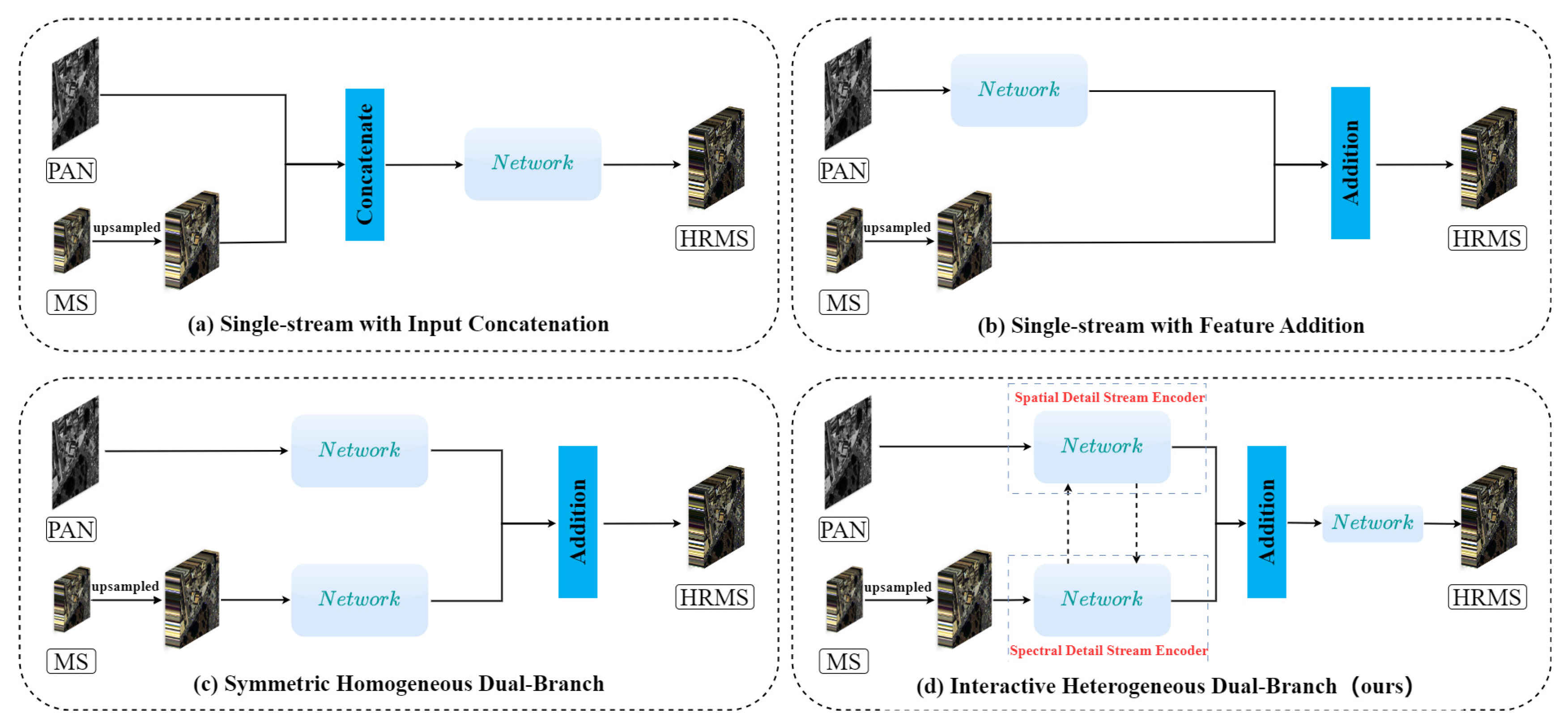
Figure 1. DL-based pansharpening framework.
Remotesensing 17 03271 g001
Figure 2. Architecture of the Hybrid Spectral–Structural Transformer Network (HSSTN).
Remotesensing 17 03271 g002
Figure 3. Detailed architecture of Self-Attention Block (SAB) and Cross-Attention Block (CAB) modules. (a) Detailed architecture of the SAB module. (b) Detailed architecture of the CAB module.
Remotesensing 17 03271 g003
Figure 4. Architecture of RBCA.
Remotesensing 17 03271 g004
Figure 5. Detailed architecture of Multi-Scale Feature Fusion (MSFF) and Pyramid Squeeze Attention (PSA) modules. (a) Detailed architecture of the MSFF module. (b) Detailed architecture of the PSA module.
Remotesensing 17 03271 g005
Figure 6. Dataset preparation process.
Remotesensing 17 03271 g006
Figure 7. Comparative visualisation of algorithms on the full-scale GaoFen-2 dataset. (a) MS. (b) PAN. (c) Brovey. (d) HPF. (e) PNN. (f) PanNet. (g) PSGAN. (h) PGMAN. (i) LDP-Net. (j) PanFormer. (k) FAFormer. (l) PLRDiff. (m) Pan-Mamba. (n) Ours.
Remotesensing 17 03271 g007
Figure 8. Comparative visualisation of algorithms on the reduced-scale GaoFen-2 dataset. (a) MS. (b) PAN. (c) Brovey. (d) HPF. (e) PNN. (f) PanNet. (g) PSGAN. (h) PGMAN. (i) LDP-Net. (j) PanFormer. (k) FAFormer. (l) PLRDiff. (m) Pan-Mamba. (n) Ours.
Remotesensing 17 03271 g008
Figure 9. Comparative visualisation of spectral residuals across algorithms on the full-scale GaoFen-2 dataset. (a) Brovey. (b) HPF. (c) PNN. (d) PanNet. (e) PSGAN. (f) PGMAN. (g) LDP-Net. (h) PanFormer. (i) FAFormer. (j) PLRDiff. (k) Pan-Mamba. (l) Ours.
Remotesensing 17 03271 g009
Figure 10. Comparative visualisation of spectral residuals across algorithms on the reduced-scale GaoFen-2 dataset. (a) Brovey. (b) HPF. (c) PNN. (d) PanNet. (e) PSGAN. (f) PGMAN. (g) LDP-Net. (h) PanFormer. (i) FAFormer. (j) PLRDiff. (k) Pan-Mamba. (l) Ours.
Remotesensing 17 03271 g010
Figure 11. Comparative visualisation of algorithms on the full-scale QuickBird dataset. (a) MS. (b) PAN. (c) Brovey. (d) HPF. (e) PNN. (f) PanNet. (g) PSGAN. (h) PGMAN. (i) LDP-Net. (j) PanFormer. (k) FAFormer. (l) PLRDiff. (m) Pan-Mamba. (n) Ours.
Remotesensing 17 03271 g011
Figure 12. Comparative visualisation of algorithms on the reduced-scale QuickBird dataset. (a) MS. (b) PAN. (c) Brovey. (d) HPF. (e) PNN. (f) PanNet. (g) PSGAN. (h) PGMAN. (i) LDP-Net. (j) PanFormer. (k) FAFormer. (l) PLRDiff. (m) Pan-Mamba. (n) Ours.
Remotesensing 17 03271 g012
Figure 13. Comparative visualisation of spectral residuals across algorithms on the full-scale QuickBird dataset. (a) Brovey. (b) HPF. (c) PNN. (d) PanNet. (e) PSGAN. (f) PGMAN. (g) LDP-Net. (h) PanFormer. (i) FAFormer. (j) PLRDiff. (k) Pan-Mamba. (l) Ours.
Remotesensing 17 03271 g013
Figure 14. Comparative visualisation of algorithms on the full-scale WorldView-3 dataset. (a) MS. (b) PAN. (c) Brovey. (d) HPF. (e) PNN. (f) PanNet. (g) PSGAN. (h) PGMAN. (i) LDP-Net. (j) PanFormer. (k) FAFormer. (l) PLRDiff. (m) Pan-Mamba. (n) Ours.
Remotesensing 17 03271 g014
Figure 15. Comparative visualisation of algorithms on the reduced-scale WorldView-3 dataset. (a) MS. (b) PAN. (c) Brovey. (d) HPF. (e) PNN. (f) PanNet. (g) PSGAN. (h) PGMAN. (i) LDP-Net. (j) PanFormer. (k) FAFormer. (l) PLRDiff. (m) Pan-Mamba. (n) Ours.
Remotesensing 17 03271 g015
Figure 16. Comparative visualisation of spectral residuals across algorithms on the full-scale WorldView-3 dataset. (a) Brovey. (b) HPF. (c) PNN. (d) PanNet. (e) PSGAN. (f) PGMAN. (g) LDP-Net. (h) PanFormer. (i) FAFormer. (j) PLRDiff. (k) Pan-Mamba. (l) Ours.
Remotesensing 17 03271 g016
Table 1. Details of the satellite datasets used in the experiments.
SensorAttributeSpecification
GaoFen-2  [60]Acquired DateAugust 2014
Area CoveredGuangzhou, China (Urban City)
Spatial ResolutionMS: 3.2 m; PAN: 0.8 m
Spectral Bands4 (Blue, Green, Red, NIR)
Bit Depth10-bit
Train SetPAN: 256 × 256 ; MS: 64 × 64 ; HRMS: 256 × 256 ; Number: 25,000
Test SetPAN: 400 × 400 ; MS: 100 × 100 ; HRMS: 400 × 400 ; Number: 286
QuickBird [61]Acquired Date18 October 2013
Area CoveredVidhansabha, Rajasthan, India
Spatial ResolutionMS: 2.40 m; PAN: 0.70 m
Spectral Bands4 (Blue, Green, Red, NIR)
Bit Depth11-bit
Train SetPAN: 256 × 256 ; MS: 64 × 64 ; HRMS: 256 × 256 ; Number: 4000
Test SetPAN: 400 × 400 ; MS: 100 × 100 ; HRMS: 400 × 400 ; Number: 32
WorldView-3 [61]Acquired Date27 November 2014
Area CoveredAdelaide, Australia
Spatial ResolutionMS: 1.20 m; PAN: 0.30 m
Spectral Bands8 (Coastal, Blue, Green, Yellow, Red, Red Edge, NIR1, NIR2)
Bit Depth11-bit
Train SetPAN: 256 × 256 ; MS: 64 × 64 ; HRMS: 256 × 256 ; Number: 18,000
Test SetPAN: 400 × 400 ; MS: 100 × 100 ; HRMS: 400 × 400 ; Number: 308
Table 2. Quantitative evaluations using different methods on the GaoFen-2 dataset.
ModelSCCERGASQ4SAMSSIMHQNR D λ D s
Brovey0.89623.48620.84152.53800.82900.85160.06670.0875
HPF0.94544.10640.86822.63280.80970.86430.03040.1086
PNN0.94501.51460.96701.72360.96360.92150.03720.0429
PanNet0.97131.33990.98141.67530.96960.89390.02890.0795
PSGAN0.95761.17360.98581.58620.97590.93840.00600.0559
PGMAN0.96761.16590.98621.90270.97120.92930.03350.0385
LDT-Net0.96591.01470.98132.34350.98620.95880.00350.0378
PanFormer0.98120.96410.99051.68040.98190.95620.23400.0209
FAFormer0.97570.92470.99120.93620.98430.97300.00750.0196
PLRDiff0.97620.93280.99151.10280.96350.98130.00680.0120
Pan-Mamba0.97850.91520.99321.16520.98710.97910.00560.0154
Ours0.98770.87890.99621.08870.98600.98080.00430.0150
Reference10101100
In the table, bolded data indicates the optimal result among all methods, while underlined data represents the second-best result.
Table 3. Quantitative evaluations using different methods on the QuickBird dataset.
ModelSCCERGASQ4SAMSSIMHQNR D λ D s
Brovey0.93412.71900.89292.30760.86000.89620.06420.0423
HPF0.95253.11260.84893.26780.84860.89240.01310.0958
PNN0.92463.34480.90203.48700.90180.90210.05180.0486
PanNet0.96331.73290.95811.79760.94350.91640.05070.0347
PSGAN0.95272.26820.94261.97560.92660.95890.02180.0197
PGMAN0.95862.10390.94982.19980.91020.97080.00420.0251
LDT-Net0.94752.10430.95052.23610.92210.93260.04680.0216
PanFormer0.97311.57260.96721.88400.92620.98130.00190.0168
FAFormer0.97481.74020.96491.79800.94990.97860.00360.0179
PLRDiff0.96511.82400.94962.00280.92670.98810.00210.0098
Pan-Mamba0.97831.60730.96921.68930.94010.97770.00530.0171
Ours0.98001.59210.97221.78890.94480.98920.00260.0082
Reference10101100
In the table, bolded data indicates the optimal result among all methods, while underlined data represents the second-best result.
Table 4. Quantitative evaluations using different methods on the WorldView-3 dataset.
ModelSCCERGASQ8SAMSSIMHQNR D λ D s
Brovey0.89833.62410.90192.46890.73900.89610.04570.0610
HPF0.90083.70120.90722.34580.86520.91620.04830.0873
PNN0.96733.37260.93062.05410.93520.90230.03150.0684
PanNet0.96933.50240.93851.56270.94830.91190.04090.0492
PSGAN0.96863.46960.92091.69230.95920.91080.04150.0498
PGMAN0.97032.96210.95711.06490.95980.95280.01760.0301
LDT-Net0.97932.87560.95291.36420.96290.90970.06090.0813
PanFormer0.97442.88890.94160.86070.96930.95700.01890.0246
FAFormer0.98572.93620.94860.85620.96970.95830.02270.0194
PLRDiff0.97922.90620.94930.87350.96090.97710.00620.0168
Pan-Mamba0.98062.68150.96080.70060.98830.95920.01950.0217
Ours0.98872.31520.96730.65290.98300.97640.00280.0209
Reference10101100
In the table, bolded data indicates the optimal result among all methods, while underlined data represents the second-best result.
Table 5. Model complexity and efficiency comparison.
ModelInference Time (s)Parameters (M)FLOPs (G)
Brovey [66]0.05--
HPF [67]0.07--
PNN [18]0.080.101.56
PanNet [34]0.090.081.22
PSGAN [37]0.132.4433.79
PGMAN [48]0.113.9112.77
LDT-Net [45]0.100.110.14
PanFormer [26]0.401.6261.01
FAFormer [68]0.342.322.69
PLRDiff [50]25.80391.055552.80
Pan-Mamba [40]0.100.4916.02
Ours0.130.386.10
Note: Inference time was benchmarked on a single NVIDIA GeForce RTX 3070 GPU. FLOPs were calculated on an image pair with a PAN size of 400 × 400.
Table 6. Comprehensive ablation study on different datasets and metrics.
QuickBirdGaoFen-2
Methods HQNR ERGAS Q4 HQNR ERGAS Q4
Ours0.98921.59210.97220.98080.87890.9962
Removal Ablation Studies
w/o RBCA0.98621.85330.96500.97830.94920.9947
w/o MSFF0.97321.72450.95320.95920.96080.9922
w/o PSA0.98041.68900.95880.96680.89920.9937
Replacement Ablation Studies
RBCA → 3 × 3 Conv0.98451.62340.96850.97650.90120.9925
MSFF → 1 × 1 Conv + Concat0.98231.64450.96680.97340.91560.9898
PSA → Spatial Attention0.98761.59340.97120.97940.88230.9952
Reference101101
“w/o” denotes removing the module, while “A → B” denotes replacing module A with B. The best results are marked in bold.
Disclaimer/Publisher’s Note: The statements, opinions and data contained in all publications are solely those of the individual author(s) and contributor(s) and not of MDPI and/or the editor(s). MDPI and/or the editor(s) disclaim responsibility for any injury to people or property resulting from any ideas, methods, instructions or products referred to in the content.