Highlights
What are the main findings?
- The highest correlation between the collocated meteor radar and MF radar wind observations are ~0.6, occurring at 82–84 km.
- The horizontal wind observations between these two instruments are more consistent during winter and spring than those during summer and autumn.
What is the implication of the main finding?
- The current analysis contributes to the accurate detection of the neutral wind in the MLT region.
- The long-term study by joint cross-device datasets also benefits from the comparative analysis of meteor radar and MF radar.
Abstract
Accurate wind measurements in the mesosphere and lower thermosphere (MLT) region are essential for climate modeling, satellite drag estimation, and space weather prediction. This study presents a comprehensive comparison and correlation analysis of the zonal and meridional wind observations from co-located meteor radar and medium-frequency (MF) radar systems in Kunming (102.1°E, 24.2°N), China, in the year 2022. Both zonal and meridional wind components were analyzed within the overlapping altitude range of 70–100 km. Statistical distributions of the wind speeds from both radars followed a near-Gaussian pattern concentrated within ±100 m/s, indicating good consistency. A joint dataset was constructed for the 78–100 km range, where over 2000 h of concurrent observations were available. The strongest correlation between the wind speed measurements of the two radars was ~0.6, which occurred near 82–84 km. Seasonal analysis further indicated better consistency in the winter and spring months, while the summer months exhibited reduced correlations, especially for zonal wind measurements. Systematic biases between the two instruments were also identified, with minimal intercept offsets observed from April to October. This study is valuable in the development of high-quality, long-term MLT wind field datasets for atmospheric research and numerical model validation.
1. Introduction
The middle and upper atmosphere, particularly the mesosphere and lower thermosphere (MLT) region at altitudes of approximately 60–100 km, serves as a crucial transitional zone between the Earth’s atmosphere and outer space. Dynamical processes in this region significantly influence spacecraft orbit maintenance, climate prediction, and space weather modeling. However, the extremely low density of air and weak signal characteristics in this region make high-precision, continuous observations difficult using traditional detection techniques. Due to relatively sparse observation methods, wind field data in the MLT region still lack effective accuracy assessment.
Meteor radars and medium-frequency (MF) radars are two important instruments for detecting zonal and meridional wind fields in the MLT region. These radars do not rely on weather conditions and have low operational and maintenance costs, making them suitable for long-term, networked observations. Standardized comparison and calibration between meteor radars and MF radars will contribute to the construction of more accurate MLT wind field datasets, thereby supporting aerospace and national defense applications.
Meteor radars typically operate in the 30–50 MHz frequency range and detect the scattering of electromagnetic waves by ionized meteor trails. Meteoroids enter the atmosphere at speeds of tens of kilometers per second, colliding with neutral molecules to generate ionized trails that form columnar plasma structures capable of reflecting radar beams. Wind velocity and direction can be retrieved from the Doppler shift in the echo signal [1]. Single-station radars generally provide only horizontal wind information, while multi-station radar networks can resolve the three-dimensional structure of the wind field. MF radars usually operate within the 1.5–5 MHz range, relying on reflections of medium-frequency electromagnetic waves by the ionosphere combined with Doppler shift measurements to detect zonal and meridional winds in the 60–100 km altitude region.
For years, zonal and meridional wind field data from meteor and MF radars have played vital roles in the study of atmospheric dynamics in the MLT region. For example, Luo et al. analyzed the diurnal and seasonal variation characteristics of sporadic meteor radiants using data from three meteor radars located in Mohe, Wuhan, and Ledong, providing insights into the origins and orbits of cosmic dust near Earth [2]. The horizontal wind observations over Mengcheng during 2015–2020 are utilized for the study of the intraseasonal variation in the mesosphere, as well as the quasi-16-day wave, which agree well with Whole Atmosphere Community Climate Model simulations [3,4]. Lima et al. investigated seasonal temperature variations over low-latitude Brazil based on meteor radar observations [5]. They found that the phase difference between equatorial temperature and wind fields (or the amplitude of diurnal tides) remained stable over time, revealing dynamic coupling processes in the tropical mesosphere through nonlinear interactions between stratospheric oscillations. Batubara et al. studied the variations in meteor peak heights over thirteen years using wind field observations from Indonesia’s meteor radar and analyzed their correlation with solar activity and sunspot numbers [6]. By comparing results with the MSISE and COSPAR IRI models, they found that daily meteor count rates can reflect upper atmospheric dynamics, and that variations in meteor peak height show a positive correlation with solar activity trends. Du et al. analyzed variations in meteor azimuth on diurnal and annual scales using data from meteor radars in Mohe and Wuhan, supplementing the understanding of azimuthal distribution features of meteors in mid-to-high latitudes and revealing characteristics of source regions linked to Earth’s rotation and revolution [7]. Dawkins et al. studied the linear trend in meteor ablation height and its response to the 11-year solar cycle using data from 12 global meteor radar stations [8]. Differences among high-latitude stations revealed the complex interaction between atmospheric variability and dynamical processes across time scales. Yi et al. used ion diffusion coefficient data from the Mengcheng meteor radar to derive 9-year mesopause temperature and relative density changes, revealing clear annual temperature cycles and the strong correlation between mesopause density structure and zonal wind variations [9]. Ratnam et al. used meteor radar data from Tirupati, India, to study echo characteristics and average wind field features in the MLT region [10]. Egito et al. extracted vertical winds over the equatorial region using meteor radar observations from São João do Cariri, Brazil, and calculated momentum fluxes carried by planetary waves, quantifying their impact on the mean atmospheric circulation [11]. Dempsey et al. investigated the altitude distribution and seasonal variability of semidiurnal and diurnal tides over Antarctica’s Rothera station, comparing the results with WACCM and ECMAM model outputs, and inferred reasons for model discrepancies [12]. Xiong et al. examined tidal structures in the MLT region using neutral wind data from Wuhan meteor radar, showing dominance of diurnal tides and significantly weaker semidiurnal and terdiurnal tides [13]. Lima used meteor radar zonal and meridional wind field data from 80 to 100 km at Cachoeira Paulista, Brazil, to investigate characteristics of the quasi-two-day wave (QTDW), finding that the QTDW is most pronounced during solstices [14], which agrees well with the QTDW results over Wuhan and Mohe [15]. Song et al. analyzed climatological features and variation patterns of the zonal and meridional winds in the MLT region using King Sejong meteor radar data and compared the results with other Antarctic stations, suggesting wind field changes may be closely correlated with gravity wave drag (GWD) variations [16]. In addition, the gravity wave activities at middle latitudes are also analyzed by Long et al. with 5-min resolution meteor radar observations over Mohe [17]. Eswaraiah et al. investigated the response of the mesosphere to a minor stratospheric sudden warming (SSW) event in February 2017 using Fukue station radar data and ERA-5 reanalysis, finding that even minor SSW events can cause significant low-latitude mesosphere responses, emphasizing the importance of middle- and low-latitude dynamics in global atmospheric circulation coupling [18]. Guharay et al. analyzed semidiurnal tide characteristics in the MLT over Maui, Hawaii, showing seasonal and altitude dependence in low-latitude semidiurnal tides [19]. Guharay et al. studied 3.5-day ultra-fast Kelvin (UFK) waves using 4-year wind data from Cachoeira Paulista, finding discrete burst-like appearances and modulation by annual cycles and harmonics [20].
Iimura et al. analyzed quasi-5-day wave (5DW) characteristics using conjugate latitude radar data from both hemispheres, revealing strong temporal and spatial variability and potential impacts on regional circulation and energy transport [21]. Guharay et al. studied solar cycle influences on dominant tides in the MLT using 1999–2018 data from Cachoeira Paulista, showing that overall tidal variation is not strongly correlated with solar activity, though the diurnal tide showed negative seasonal correlation [22]. Pancheva et al. analyzed climatological wind data, diurnal tides (DTs), and semidiurnal tides (SDTs) from meteor radars in Svalbard and Tromsø, revealing significant differences in DT seasonal and vertical structures despite geographic proximity [23]. Guo et al. used JASMET radar data to study vertical structures and seasonal variability of tides at 80–100 km [24]. John et al. compared zonal wind diurnal variations from TIMED/TIDI and Thumba radar to validate meteor radar wind measurements near EEJ heights [25]. Namboothiri et al. characterized MLT zonal and meridional wind fields from MF radars at Yamagawa and Wakkanai [26], while Xiao et al. analyzed MLT wind structures near 30°N using data from Wuhan and Yagihara, simulated by the 2D-SOCRATES model [27]. Ramkumar et al. found significant electrodynamic interference in MF radar wind measurements near the EEJ [28]. Namboothiri et al. studied terdiurnal tides at Wakkanai and compared them with London, Ontario data, revealing strong diurnal variation and weak seasonal variation [29]. Manson et al. combined optical and MF radar data from 1991 to 1998 to investigate Airglow Springtime Transition (AST) features [30]. Tomikawa et al. analyzed diurnal tide characteristics using 10 years of MF radar data from Syowa Station, Antarctica [31]. Sridharan et al. used Rayleigh lidar temperature data from Gadanki and MF radar wind data from Tirunelveli to study tidal–gravity wave interactions forming Mesospheric Inversion Layers (MILs) [32]. Hibbins et al. used Rothera MF radar to reveal periodic (≤1 day) wind variations and gravity wave–background wind interactions [33]. Kishore et al. analyzed MLT mean wind and solar tides from Poker Flat MF radar, verifying its reliability in polar observations [34]. McDonald applied Empirical Mode Decomposition (EMD) to separate components in wind observations from Scott Base MF radar [35]. Manson et al. compared long-term MF radar data with GSWM and CMAM models, validating tidal physics and gravity wave parameterizations [36]. Hocke et al. analyzed climatological features of mean winds and tides using MF radar data from Wakkanai and Yamagawa [37]. Vincent et al. studied interannual variability of solar tides using MF radar wind data from Adelaide, Christmas Island, and Kauai [38]. Krishnapriya et al. analyzed high-frequency gravity wave activity associated with Tropical Cyclone Vayu in June 2019 using MF radar data from Kolhapur, showing vertical coupling between the lower and upper atmosphere via gravity wave propagation [39]. Hoffmann et al. used zonal and meridional wind field data from Juliusruh and Andenes (meteor and MF radar), along with high-resolution general circulation model simulations, to investigate seasonal variability in MLT wave activity [40].
Due to the rarity of co-located meteor and MF radar deployments, comparative studies using joint observations are limited. The Geophysical Observatories in Kunming and Langfang have both meteor and MF radars operating simultaneously and continuously. This study uses one consecutive year (2022) of co-located data from Kunming station to conduct a comparative analysis of meteor and MF radar observations, aiming to reveal intrinsic differences and regional dependencies between the two measurement techniques. The current analysis results are valuable in the development of high-quality, long-term MLT wind field datasets for atmospheric research and numerical model validation, which is also usable for the usage of these observations for scientific research.
2. Data Processing and Analysis Methods
The data used in this study were obtained from meteor and MF radars deployed in the Kunming station (102.1°E, 24.2°N), which independently measured the zonal and meridional wind fields. The dataset spans from 00:00 on January 1 to 23:00 on December 31, 2022, with a temporal resolution of 1 h and a vertical resolution of 2 km. It is noteworthy that the meteor radar primarily observes higher altitudes, covering the 70–100 km range, whereas the MF radar operates over a broader but generally lower altitude range of 50–100 km.
As shown in Table 1, the overlapping detection altitude range of the meteor radar and the MF radar is 70–100 km. The wind field measurements within this common altitude range in 2022, including the zonal and meridional winds observed by both MF and MR radar, are illustrated in Figure 1 and Figure 2.

Table 1.
The system paramters for meteor radar and MF radar at Kunming.
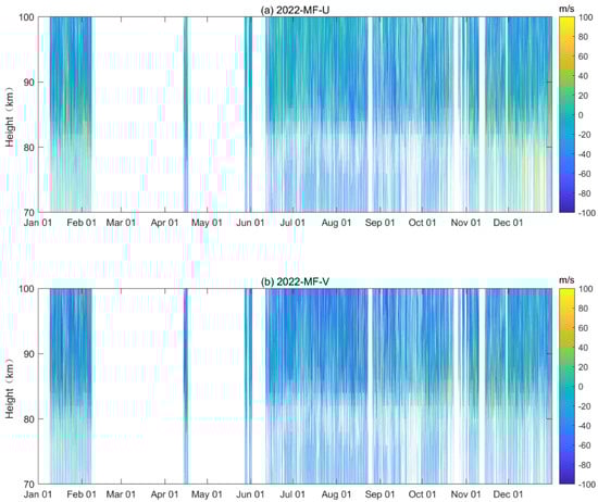
Figure 1.
Observations of the zonal wind (a) and meridional wind (b) made by the MF radar in 2022.
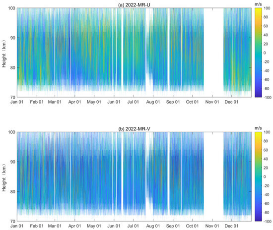
Figure 2.
Observations of the zonal wind (a) and meridional wind (b) made by the meteor radar in 2022.
Figure 1 presents the MF radar observations of the wind field over Kunming from 00:00 on 1 January to 23:00 on 31 December 2022. Figure 1a shows the zonal wind field, while Figure 1b shows the meridional wind field. The x-axis represents time, with tick marks indicating the first hour of the first day of each month, and the y-axis represents altitude, ranging from 70 km to 100 km. The color bar indicates wind speed (m/s), where positive values denote eastward zonal winds or northward meridional winds, and negative values denote westward zonal winds or southward meridional winds. White gaps in the figures indicate periods of missing data. Overall, the data gaps in the meridional and zonal wind fields show similar characteristics. In terms of temporal distribution, the MF radar data show fewer gaps in the second half of 2022, whereas the first half exhibits more severe data loss. Specifically, extensive data gaps across the entire altitude range are observed during early January, from mid-February to mid-April, late April to late May, and early June. Regarding altitude distribution, the 80–100 km range shows relatively fewer data gaps, while data below 80 km are more frequently missing.
Figure 2 illustrates the zonal and meridional wind field observations obtained by the meteor radar over Kunming for the same period and altitude range as in Figure 1. Panel (a) displays the zonal wind, while panel (b) presents the meridional wind. A comparison between Figure 1 and Figure 2 reveals notable differences in the data availability characteristics between the two radar systems. In terms of temporal distribution, the meteor radar exhibited fewer data gaps in both zonal and meridional wind measurements during the first half of 2022, whereas more significant data loss occurred in the second half of the year—particularly from mid-October to mid-November, during which a complete absence of data was observed across all altitudes. Regarding vertical distribution, the meteor radar showed relatively fewer missing data points in the 74–100 km altitude range, while more frequent data gaps were observed below 74 km. Moreover, it is evident that the meteor radar, compared with the MF radar, experienced less overall data loss and delivered higher-quality wind measurements throughout the year.
Subsequently, this study conducted a quantitative statistical analysis of the zonal and meridional wind speed distributions measured by the MF and the meteor radars at Kunming station in the overlapping altitude range during 2022. Specifically, the wind speed range for each radar (from minimum to maximum) was evenly divided into 50 equal-width bins, and the number of data points falling within each bin was counted. The statistical results are shown in Figure 3 and Figure 4.
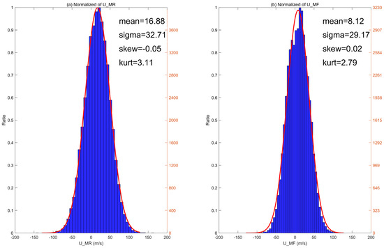
Figure 3.
Zonal wind distributions observed by (a) the meteor radar and (b) the MF radar.
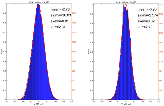
Figure 4.
Meridional wind distributions observed by the meteor radar (a) and the MF radar (b).
Figure 3 presents the distribution of zonal wind speeds observed by the meteor radar and the MF radar over Kunming in the 70–100 km altitude range in 2022. Figure 3a shows the results from the meteor radar, and Figure 3b shows those from the MF radar. The x-axis represents wind speed, with positive values indicating eastward winds and negative values indicating westward winds, while the y-axis represents the number of observations. Blue and red bars represent the number of data points within each wind speed bin. A comparison of Figure 3a,b reveals that the meteor radar exhibits a wider wind speed range (−150 to 150 m/s), whereas the MF radar’s range is relatively narrower (−100 to 130 m/s). In addition, both radars’ zonal wind speed distributions show a generally normal (Gaussian) distribution pattern, with the majority of data points concentrated within the −100 to 100 m/s range. The Gaussian fitting analysis shows that the mean zonal wind of the meteor radar observations during 2022 is ~16.88 m/s with a standard deviation of 32.71 m/s. In addition, the skewness and kurtosis of the meteor radar zonal wind distribution are −0.05 and 3.11, respectively. As a comparison, the Gaussian fitting analysis of the MF zonal wind shows a mean value of 8.12 m/s with a standard deviation of 29.17 m/s during 2022. In addition, the skewness and kurtosis of the MF zonal wind distribution are 0.02 and 2.79, respectively.
Figure 4 shows the meridional wind speed distributions observed by the meteor radar and the MF radar over Kunming at 70–100 km in 2022. Figure 4a corresponds to the meteor radar, and Figure 4b to the MF radar. As in the zonal case, the meridional wind speeds measured by the meteor radar cover a broader range (−150 to 150 m/s), while the MF radar ranges from −150 to 120 m/s. Again, the wind speed distributions of the meridional wind field generally conform to a normal distribution, with most values falling within the −100 to 100 m/s interval. Considering potential systematic and random errors inherent in both radar systems and the observational processes, which may lead to extreme deviations in wind speed measurements, this study focuses on wind data within the concentrated range of −100 to 100 m/s from both the meteor and MF radars for subsequent cross-comparison and analysis. The Gaussian fitting analysis shows that the mean meridional wind of the meteor radar observations during 2022 is −2.78 m/s with a standard deviation of 36.03 m/s. In addition, the skewness and kurtosis of the meteor radar meridional wind distribution are −0.01 and 2.81, respectively. As a comparison, the Gaussian fitting analysis of the MF meridional wind shows a mean value of −0.96 m/s with a standard deviation of 27.74 m/s during 2022. In addition, the skewness and kurtosis of the MF meridional wind distribution are 0.02 and 2.79, respectively.
3. Results
By comparing Figure 1 and Figure 2, it can be observed that the distribution of missing detection values in terms of height and time differs significantly between the MF radar and the meteor radar. To minimize errors and conduct more effective subsequent cross-comparison analysis, this study counted the number of observation points with simultaneous zonal and meridional wind field data from both radars in 2022, at 16 fixed altitudes with a vertical resolution of 2 km, within the 70–100 km height range. The results are shown in Figure 5.
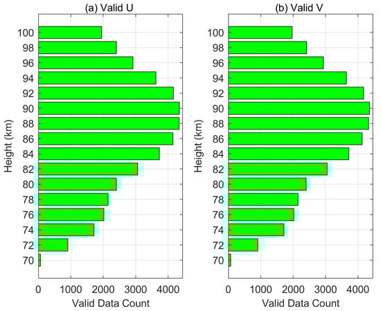
Figure 5.
Vertical distribution of the zonal wind (a) and meridional wind (b) from the coincident observations in 2022.
Figure 5 presents the distribution of the jointly observed data volume from the MF radar and the meteor radar in the 70–100 km height range in 2022. Figure 5a shows the zonal wind results, and Figure 5b shows the meridional wind results. A comparison of Figure 5a,b reveals that the statistical results for the meridional and zonal wind fields are almost identical. The jointly observed data volume from both radars shows an increasing trend followed by a decreasing trend with height. The minimum joint data volume occurs at 70 km, with less than 200 h of observation, while the maximum joint data volume occurs at 90 km, exceeding 4000 h.
Furthermore, Figure 5 also indicates that in the 78–100 km height range, the joint observation data volume from both radars exceeds 2000 h, suggesting that both radars can conduct relatively stable observations in this height range, with higher data quality, making it suitable for subsequent cross-comparison analysis. Notably, in the 86–92 km altitude range, the joint observation data volume exceeds 4000 h, indicating that the observation data in this range has high reliability and representativeness.
A correlation analysis was conducted for the data jointly detected from the meteor and MF radars in the 78–100 km height range; the results are shown in Figure 6, Figure 7, Figure 8 and Figure 9. Figure 6 shows the correlation between the zonal wind field data observed by the meteor and MF radars at different heights. The x-axis represents the zonal wind speed detected by the meteor radar, and the y-axis represents the zonal wind speed detected by the MF radar. Both units are in m/s. The red solid line in the figure represents the fitted line calculated using the least squares method. To quantitatively determine the distribution of the correlation between the two sets of detection data with height, this study calculated and statistically analyzed the slope and intercept of the fitted line at the 12 heights mentioned above. The results of these calculations are shown in Figure 7.
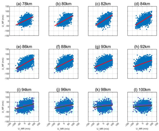
Figure 6.
Linear fitting results of zonal wind recorded at different heights by the meteor and MF radars in 2022. The dots represent the coindicent wind observations be meteor radar and MF radar, and red lines are the lienar fitting results.
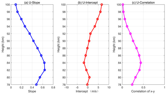
Figure 7.
Distributions of slopes (a), intercepts (b), and correlation coefficients (c) for the linear fitting of zonal wind at different heights.
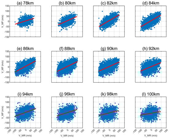
Figure 8.
Linear fitting results of meridional wind recorded at different heights by the meteor and MF radars in 2022. The dots represent the coindicent wind observations be meteor radar and MF radar, and red lines are the lienar fitting results.
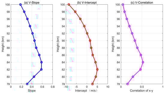
Figure 9.
Distributions of slopes (a), intercepts (b) and correlation coefficients (c) for the linear fitting of meridional wind at different heights.
Figure 7 shows the distribution of the slope and intercept values of the fitted line for the zonal wind field data at different heights. Figure 7a shows the distribution of the slope of the fitted line with height, where the x-axis represents the slope values, and the y-axis represents height (in km). Figure 7b shows the distribution of the intercept of the fitted line with height, where the x-axis represents the intercept values, with units in m/s. Combining Figure 6 and Figure 7 indicates that the slope of the fitted line shows an increasing trend with height, followed by a decreasing trend, indicating that the correlation between the meteor radar and MF radar joint detection data first increases and then decreases with height. The maximum slope value occurs at 82 km, reaching approximately 0.64, and the minimum slope occurs at 100 km, with a value of approximately 0.09.
Furthermore, Figure 7b shows that the intercept of the fitted line for the zonal wind joint detection data generally increases with height. In the 78–88 km height range, the intercept fluctuates around 0, with a trough value of approximately −1.83 m/s at 84 km. At this height, the deviation between the meteor radar and MF radar detection is minimal. Above 88 km, the intercept shows an increasing trend with height, reaching a peak value of approximately 6.6 m/s at 100 km, indicating that the deviation between the two radars increases with height. Figure 7c shows the height variations in the zonal wind correlation coefficients between meteor and MF radar observations. The highest correlation of ~0.45 are found to be at 84 km, and the correlation coefficients at 82 and 86 km reaches ~0.4, which are only slightly smaller than the peak value at 84 km. In addition, we found that the higher correlation coefficients are observed where the zonal wind observations from these two instruments are more consistent with each other (Figure 7a).
Figure 8 shows the correlation between the meridional wind field data jointly observed by the meteor and MF radars at different heights. The x-axis represents the meridional wind speed detected by the meteor radar, and the y-axis represents the meridional wind speed detected by the MF radar, with both units in m/s. The red solid line in the figure represents the fitted line calculated using the least squares method. Similarly to the zonal wind field, the slope and intercept of the fitted line for the meridional wind field at different heights were also calculated, and the results are shown in Figure 9.
Figure 9 shows the distribution of the slope and intercept values of the fitted line for the meridional wind joint detection data with height. Figure 9a shows the distribution of the slope of the fitted line with height, where the x-axis represents the slope values, and the y-axis represents height (in km). Figure 9b shows the distribution of the intercept of the fitted line with height, where the x-axis represents the intercept values, with units in m/s.
Comparing Figure 8 and Figure 9 shows that the slope of the fitted line for the meridional wind field shows a similar trend to the slope for the zonal wind field in Figure 7a—it increases and then decreases with height. This indicates that the correlation of the joint detection data between the meteor and MF radars for the meridional wind field first increases and then decreases with height. The maximum slope value occurs at 84 km, with a peak value of approximately 0.59, and the minimum slope occurs at 100 km, with a value of approximately 0.18.
Figure 9b shows that the intercept of the fitted line for the meridional wind joint detection data first increases and then decreases with height. In the 78–92 km height range, the intercept is greater than 0, reaching a peak value of approximately 5.02 m/s at 82 km. In the 92–100 km height range, the intercept is less than 0, with a trough value of approximately −8.65 m/s at 100 km. The intercept is 0 at 92 km, indicating that the fixed deviation between the meteor radar and MF radar detection is minimal at this height. Figure 9c shows the height variations in the meridional wind correlation coefficients between meteor and MF radar observations, which shows similar vertical trend as the zonal component. The highest correlation of ~0.52 is found to be at 84 km, and the correlation coefficients at 82 and 86 km reaches ~0.48. We found that the higher correlation coefficients for meridional wind are also observed where the wind observations of these two instruments are more consistent with each other (Figure 9a).
Next, the distribution of the joint detection data from the MF and meteor radars in 2022 across the 78–100 km height range was statistically analyzed by month; the results are shown in Figure 10.
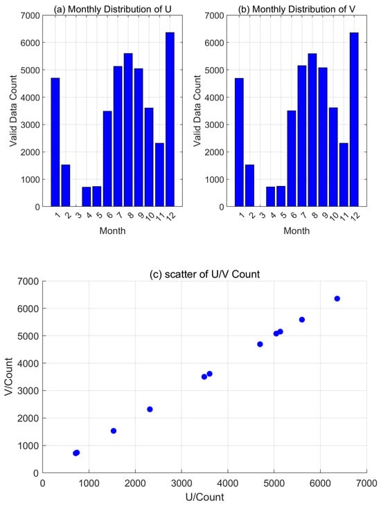
Figure 10.
Monthly statistics of zonal wind (a), meridional wind (b), and their relationship (c) from meteor radar and MF radar observation in 2022.
Figure 10 shows the distribution of the joint observation data volume from the MF and meteor radars in the 78–100 km height range across months in 2022. Figure 10a shows the zonal wind results, and Figure 10b shows the meridional wind results. The x-axis represents the months, and the y-axis represents the number of data points.
Comparing Figure 10a,b shows that the data volume distribution for the meridional wind field and the zonal wind field follows a nearly identical pattern across months. The joint observation data volume is smaller in the first half of the year and larger in the second half. It is noteworthy that the joint observation data volume peaks in December, exceeding 6000, while the joint observation data for March is 0, which corresponds to the full-height data gap for March observed by the MF radar in Figure 1. Additionally, Figure 10 shows that the joint observation data volume from February to May is less than 2000 h, indicating that the data quality during this period is relatively low. Figure 10c shows that the valid zonal and meridional wind observations utilized in the analysis are consistent during the whole year, which indicates that the operation of these two instruments are stable during 2022 and the statistical analysis results are reliable.
A correlation analysis of the joint detection data from the meteor and MF radars in the 78–100 km height range for 2022 was performed by month, and the results are shown in Figure 11, Figure 12, Figure 13 and Figure 14.
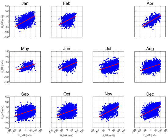
Figure 11.
Linear fitting results of the zonal wind observed by the meteor and MF radars in different months in 2022.
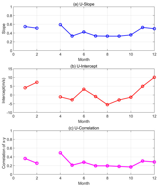
Figure 12.
Variations in the slopes (a), intercepts (b) and the correlation coefficients (c) for the linear fitting of the zonal wind field during different months.
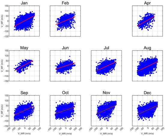
Figure 13.
Linear fitting results of the meridional wind observed by the meteor and MF radars in different months in 2022.
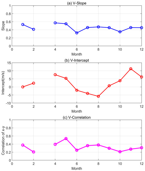
Figure 14.
Variations in the slopes (a), intercepts (b) and the correlation coefficients (c) for the linear fitting of the meridional wind field during different months.
Figure 11 shows the correlation between the zonal wind field jointly observed by the meteor and MF radars in different months. The x-axis represents the zonal wind speed detected by the meteor radar, and the y-axis represents the zonal wind speed detected by the MF radar, with units in m/s. The red solid line represents the fitted line calculated using the least squares method.
To investigate the distribution characteristics of the correlation between the joint detection data from both radars across months, the slopes, and intercepts of the fitted lines were calculated and statistically analyzed for all 12 months. Figure 12 shows the distribution of the slope and intercept of the fitted lines for the zonal wind joint observation data across months. Figure 12a shows the distribution of the slope of the fitted line across months, with the x-axis representing the months and the y-axis representing the slope. Figure 12b shows the distribution of the intercept of the fitted line across months, with the y-axis representing the intercept in m/s.
Examining Figure 11 and Figure 12 shows that the slope of the fitted line for the zonal wind field is lower from May to October, generally below 0.5, indicating that the correlation between the MF radar and meteor radar results is relatively weak in the summer and fall. However, from January to April and in November and December, the slope is higher than 0.5, suggesting a stronger correlation between the joint observations during the spring and winter months. The slope reaches its peak in April at approximately 0.59 and its minimum in May at approximately 0.33. Additionally, Figure 12b shows that the intercept of the fitted line for the zonal wind joint detection data fluctuates around 0 m/s from April to October, indicating a smaller fixed bias between the meteor and MF radars in the middle of the year. In contrast, from January to February and in November and December, the intercept is generally larger, suggesting a greater fixed bias between the two radars at the beginning and end of the year. The intercept reaches a peak of approximately 10.11 m/s in December and a trough of approximately −5.52 m/s in August. Figure 12c shows that the correlation between the zonal wind observations from meteor and MF radar is maximum during April, which is ~0.5. The correlation coefficients are ~0.4, ~0.3 and ~0.3 for January, November, and December, respectively. The correlation coefficients during other months are only ~0.2.
Figure 13 shows the correlation between the joint observation data of the meridional wind field from the meteor and MF radars in different months. The x-axis represents the meridional wind speed detected by the meteor radar, and the y-axis represents the meridional wind speed detected by the MF radar, with both units in m/s. The red solid line represents the fitted line calculated using the least squares method.
Similarly, for the meridional wind field, the slope and intercept of the fitted line were calculated for each month; the results are shown in Figure 14. Figure 14 displays the distribution of the slope and intercept of the fitted lines for the meridional wind joint observation data across months. Figure 14a shows the distribution of the slope of the fitted line across months, with the x-axis representing the months and the y-axis representing the slope. Figure 14b shows the distribution of the intercept of the fitted line across months, with the y-axis representing the intercept in m/s.
Examining Figure 13 and Figure 14 shows that the slope of the fitted line for the meridional wind field is only below 0.4 in June and October, with little variation across months. Compared with Figure 12a, the meridional wind fitted slope is generally higher than the zonal wind slope, indicating that the correlation between the MF radar and meteor radar results for meridional wind detection is stronger than that for zonal wind detection. The meridional wind fitted slope reaches its peak in April at approximately 0.57 and its minimum in June at approximately 0.32. Additionally, Figure 14b shows that the intercept of the fitted line for the meridional wind field exhibits a clear oscillatory trend with a period of approximately 270 days. The intercept first increases, then decreases, and then increases again with the passage of months. In January, May, and September, the intercept is close to 0 m/s. In April, the peak value is approximately 7.59 m/s, in August, the trough is approximately −5.82 m/s, and in November, the peak value reaches approximately 11.26 m/s. Figure 14c shows that the correlation between the meridional wind observations from meteor and MF radar is maximum during May, which is ~0.5. The correlation coefficients are ~0.4 during January, April, July and August. The correlation coefficients during other months are only ~0.2–0.3.
4. Discussion and Conclusions
This study systematically analyzes the differences and consistencies between meteor radar and medium-frequency radar in detecting zonal and meridional wind fields in the middle and upper atmosphere, within the altitude range of 70–100 km, based on joint observation data from 2022 in the Kunming region. The analysis covers various dimensions, including overall wind speed distribution, time–altitude detection differences, the distribution of co-observation data with altitude and season, and wind field correlations. The results indicate the following:
- 1.
- Significant differences in observation coverage characteristics: The meteor radar exhibits better data completeness throughout the year, particularly in the altitude range of 74–100 km, with higher detection stability; in contrast, the medium-frequency radar shows significant data gaps below 80 km.
- 2.
- Good consistency in wind speed distribution statistics: Both instruments observe zonal and meridional wind speeds, which generally follow a normal distribution, mainly concentrated in the range of −100 to 100 m/s, demonstrating good comparability.
- 3.
- Altitude and seasonal dependence of co-observation data: The two radars show the best consistency at the altitude range of 78–100 km, particularly between 86 and 92 km, where the co-observation time exceeds 4000 h. In terms of time, more co-observed data are available in summer and autumn, with the least amount of data in spring.
- 4.
- Altitude and seasonal differences in wind field fitting correlation: The altitude analysis reveals that the correlation between the two radars is strongest at 82–84 km, with the correlation decreasing with altitude. Seasonal analysis shows that the correlation of zonal wind is higher in spring and winter and lowest in summer, while the meridional wind correlation is relatively more stable. We speculate that the height variation in the linear fitting results are likely related to the measurement principles of these two radars, while the seasonal variations in the fitting results are possibly related to the weather conditions during different seasons. This needs verification with a longer dataset.
- 5.
- Regular pattern of fixed bias: The analysis of fitting intercepts reveals that both instruments exhibit some systematic biases in wind speed observation, especially at the beginning and the end of the year, with smaller biases between April and October, providing a basis for subsequent unified correction. However, the variations in the systematic bias are not totally understood.
Reid et al. shows that the ratio between MF radar and meteor radar is ~0.7 at Davis Station in the Australis, which is slightly larger than the current analysis results [41]. This is possibly due to different meteor injection and ion scattering at these two stations. Nevertheless, both Reid et al. [41] and Wilhelm et al. [42] showed that neutral winds are underestimated by MF radar than that by meteor radar. In fact, Hall et al. pointed out that the comparison results between MF and meteor radars may well depend on geographic location, surface topology and also season since mean winds affect gravity wave filtering and therefore momentum deposition in the middle atmosphere [43,44].
In conclusion, meteor and medium-frequency radars complement each other in the detection of middle and upper atmospheric wind fields. The altitude range of 86–92 km, where the joint observation data is abundant and of high quality, is suitable for cross-comparison and calibration as the core layer. The systematic comparison and consistency evaluation of the observation data from both instruments contribute to the construction of high-quality and continuous wind field datasets for the middle and upper atmosphere with multiple instruments, providing important references and support for studies in middle atmospheric dynamics, global circulation model calibration, and climate change research.
Author Contributions
Conceptualization, X.W.; Data curation, Z.D.; Investigation, N.L.; Writing—original draft, Y.G. All authors have read and agreed to the published version of the manuscript.
Funding
This project was funded by the Postdoctoral Project of Hubei Province (Grant Number 2024HBBHCXA054).
Data Availability Statement
Meteor and MF radar data can be found at https://data2.meridianproject.ac.cn/ (accessed on 1 September 2025).
Acknowledgments
All the authors acknowledge the Chinese Meridian Project for providing Meteor and MF radar data.
Conflicts of Interest
The authors declare no conflicts of interest.
References
- Reid, I.M. Meteor Radar for Investigation of the MLT Region: A Review. Atmosphere 2024, 15, 505. [Google Scholar] [CrossRef]
- Luo, J.; Gong, Y.; Zhang, S.; Zhou, Q.; Ma, Z. Seasonal variations in the strength of sporadic meteor sources observed by meteor radar. J. Geophys. Res. Space Phys. 2025, 130, e2024JA033618. [Google Scholar] [CrossRef]
- Tang, Y.; Hao, X.; Qiu, S.; Cheng, W.; Yang, C.; Wu, J. Intraseasonal Variation in the Mesosphere Observed by the Mengcheng Meteor Radar from 2015 to 2020. Atmosphere 2023, 14, 1034. [Google Scholar] [CrossRef]
- Yang, C.; Lai, D.; Yi, W.; Wu, J.; Xue, X.; Li, T.; Chen, T.; Dou, X. Observed Quasi 16-Day Wave by Meteor Radar over 9 Years at Mengcheng (33.4°N, 116.5°E) and Comparison with the Whole Atmosphere Community Climate Model Simulation. Remote Sens. 2023, 15, 830. [Google Scholar] [CrossRef]
- Lima, L.M.; Batista, P.P.; Paulino, A.R. Meteor radar temperatures over the Brazilian low-latitude sectors. J. Geophys. Res. Space Phys. 2018, 123, 7755–7766. [Google Scholar] [CrossRef]
- Batubara, M.; Yamamoto, M.Y.; Madkour, W.; Manik, T. Long-term distribution of meteors in a solar cycle period observed by VHF meteor radars at near-equatorial latitudes. J. Geophys. Res. Space Phys. 2018, 123, 10403–10415. [Google Scholar] [CrossRef]
- Du, X.; Yin, W.; Du, Z.; Zhou, Y.; Feng, J.; Xu, B.; Xu, T.; Deng, Z.; Zhao, Z.; Zhang, Y.; et al. Distribution Characteristics of Meteor Angle of Arrival in Mohe and Wuhan, China. Atmosphere 2023, 14, 1431. [Google Scholar] [CrossRef]
- Dawkins, E.C.M.; Stober, G.; Janches, D.; Carrillo-Sánchez, J.D.; Lieberman, R.S.; Jacobi, C.; Moffat-Griffin, T.; Mitchell, N.J.; Cobbett, N.; Batista, P.P.; et al. Solar cycle and long-term trends in the observed peak of the meteor altitude distributions by meteor radars. Geophys. Res. Lett. 2023, 50, e2022GL101953. [Google Scholar] [CrossRef]
- Yi, W.; Xue, X.; Lu, M.; Zeng, J.; Ye, H.; Wu, J.; Wang, C.; Chen, T. Mesopause temperatures and relative densities at midlatitudes observed by the Mengcheng meteor radar. Earth Planet. Phys. 2023, 7, 665–674. [Google Scholar] [CrossRef]
- Ratnam, M.V.; Teja, A.K.; Pramitha, M.; Eswaraiah, S.; Rao, S.V.B. Climatology of meteor echoes and mean winds in the MLT region revealed by SVU meteor radar over Tirupati (13.63°N, 79.4°E): Long-term trends. Adv. Space Res. 2025, 75, 4768–4785. [Google Scholar] [CrossRef]
- Egito, F.; Andrioli, V.F.; Batista, P.P. Vertical winds and momentum fluxes due to equatorial planetary scale waves using all-sky meteor radar over Brazilian region. J. Atmos. Sol.-Terr. Phys. 2016, 149, 108–119. [Google Scholar] [CrossRef]
- Dempsey, S.M.; Hindley, N.P.; Moffat-Griffin, T.; Wright, C.J.; Smith, A.K.; Du, J.; Mitchell, N.J. Winds and tides of the Antarctic mesosphere and lower thermosphere: One year of meteor-radar observations over Rothera (68°S, 68°W) and comparisons with WACCM and eCMAM. J. Atmos. Sol.-Terr. Phys. 2021, 212, 105510. [Google Scholar] [CrossRef]
- Xiong, J.G.; Wan, W.; Ning, B.; Liu, L. First results of the tidal structure in the MLT revealed by Wuhan meteor radar (30°40′N, 114°30′E). J. Atmos. Sol.-Terr. Phys. 2004, 66, 675–682. [Google Scholar] [CrossRef]
- Lima, L.M.; Batista, P.P.; Takahashi, H.; Clemesha, B.R. Quasi-two-day wave observed by meteor radar at 22.7°S. J. Atmos. Sol.-Terr. Phys. 2004, 66, 529–537. [Google Scholar] [CrossRef]
- Tang, L.; Gu, S.-Y.; Sun, R.; Dou, X. Multi-Year Behavioral Observations of Quasi-2-Day Wave Activity in High-Latitude Mohe (52.5°N, 122.3°E) and Middle-Latitude Wuhan (30.5°N, 114.6°E) Using Meteor Radars. Remote Sens. 2024, 16, 311. [Google Scholar] [CrossRef]
- Song, B.G.; Chun, H.Y.; Song, I.S.; Lee, C.; Kim, J.H.; Jee, G. Long-term characteristics of the meteor radar winds observed at King Sejong station, Antarctica. J. Geophys. Res. Atmos. 2023, 128, e2022JD037190. [Google Scholar] [CrossRef]
- Long, C.; Yu, T.; Sun, Y.-Y.; Yan, X.; Zhang, J.; Yang, N.; Wang, J.; Xia, C.; Liang, Y.; Ye, H. Atmospheric Gravity Wave Derived from the Neutral Wind with 5-Minute Resolution Routinely Retrieved by the Meteor Radar at Mohe. Remote Sens. 2023, 15, 296. [Google Scholar] [CrossRef]
- Eswaraiah, S.; Kumar, K.N.; Kim, Y.H.; Chalapathi, G.V.; Lee, W.; Jiang, G.; Yan, C.; Yang, G.; Ratnam, M.V.; Prasanth, P.V.; et al. Low-latitude mesospheric signatures observed during the 2017 sudden stratospheric warming using the fuke meteor radar and ERA-5. J. Atmos. Sol.-Terr. Phys. 2020, 207, 105352. [Google Scholar] [CrossRef]
- Guharay, A.; Franke, S.J. Characteristics of the semidiurnal tide in the MLT over Maui (20.75°N, 156.43°W) with meteor radar observations. J. Atmos. Sol.-Terr. Phys. 2011, 73, 678–685. [Google Scholar] [CrossRef]
- Guharay, A.; Batista, P.P.; Clemesha, B.R. Study of the ultra-fast Kelvin wave with meteor radar observations over a Brazilian extra-tropical station. J. Atmos. Sol.-Terr. Phys. 2013, 102, 115–124. [Google Scholar] [CrossRef]
- Iimura, H.; Fritts, D.C.; Janches, D.; Singer, W.; Mitchell, N.J. Interhemispheric structure and variability of the 5-day planetary wave from meteor radar wind measurements. Ann. Geophys. 2015, 33, 1349–1359. [Google Scholar] [CrossRef][Green Version]
- Guharay, A.; Batista, P.P.; Andrioli, V.F. Investigation of solar cycle dependence of the tides in the low latitude MLT using meteor radar observations. J. Atmos. Sol.-Terr. Phys. 2019, 193, 105083. [Google Scholar] [CrossRef]
- Pancheva, D.; Mukhtarov, P.; Hall, C.; Meek, C.; Tsutsumi, M.; Pedatella, N.; Nozawa, S. Climatology of the main (24-h and 12-h) tides observed by meteor radars at Svalbard and Tromsø: Comparison with the models CMAM-DAS and WACCM-X. J. Atmos. Sol.-Terr. Phys. 2020, 207, 105339. [Google Scholar] [CrossRef]
- Guo, L.; Lehmacher, G. First meteor radar observations of tidal oscillations over Jicamarca (11.95°S, 76.87°W). Ann. Geophys. 2009, 27, 2575–2583. [Google Scholar] [CrossRef]
- John, S.R.; Kumar, K.K.; Subrahmanyam, K.V.; Manju, G.; Wu, Q. Meteor radar measurements of MLT winds near the equatorial electro jet region over Thumba (8.5°N, 77°E): Comparison with TIDI observations. Ann. Geophys. 2011, 29, 1209–1214. [Google Scholar] [CrossRef]
- Namboothiri, S.P.; Kishore, P.; Igarashi, K.; Nakamura, T.; Tsuda, T. MF radar observations of mean winds over Yamagawa (31.2°N, 130.6°E) and Wakkanai (45.4°N, 141.7°E). J. Atmos. Sol.-Terr. Phys. 2000, 62, 1177–1187. [Google Scholar] [CrossRef]
- Xiao, C.Y.; Hu, X.; Zhang, X.X.; Zhang, D.Y.; Wu, X.C.; Gong, X.Y.; Igarashi, K. Interpretation of the mesospheric and lower thermospheric mean winds observed by MF radar at about 30 N with the 2D-SOCRATES model. Adv. Space Res. 2007, 39, 1267–1277. [Google Scholar] [CrossRef]
- Ramkumar, T.K.; Gurubaran, S.; Rajaram, R. Lower E-region MF radar spaced antenna measurements over magnetic equator. J. Atmos. Sol.-Terr. Phys. 2002, 64, 1445–1453. [Google Scholar] [CrossRef]
- Namboothiri, S.P.; Kishore, P.; Murayama, Y.; Igarashi, K. MF radar observations of terdiurnal tide in the mesosphere and lower thermosphere at Wakkanai (45.4°N, 141.7°E), Japan. J. Atmos. Sol.-Terr. Phys. 2004, 66, 241–250. [Google Scholar] [CrossRef]
- Manson, A.H.; Meek, C.E.; Stegman, J.; Espy, P.J.; Roble, R.G.; Hall, C.M.; Hoffmann, P.; Jacobi, C. Springtime transitions in mesopause airglow and dynamics: Photometer and MF radar observations in the Scandinavian and Canadian sectors. J. Atmos. Sol.-Terr. Phys. 2002, 64, 1131–1146. [Google Scholar] [CrossRef]
- Tomikawa, Y.; Tsutsumi, M. MF radar observations of the diurnal tide over Syowa, Antarctica (69°S, 40°E). Ann. Geophys. 2009, 27, 2653–2659. [Google Scholar] [CrossRef]
- Sridharan, S.; Sathishkumar, S.; Gurubaran, S. Influence of gravity waves and tides on mesospheric temperature inversion layers: Simultaneous Rayleigh lidar and MF radar observations. Ann. Geophys. 2008, 26, 3731–3739. [Google Scholar] [CrossRef]
- Hibbins, R.E.; Espy, P.J.; Jarvis, M.J.; Riggin, D.M.; Fritts, D.C. A climatology of tides and gravity wave variance in the MLT above Rothera, Antarctica obtained by MF radar. J. Atmos. Sol.-Terr. Phys. 2007, 69, 578–588. [Google Scholar] [CrossRef]
- Kishore, P.; Namboothiri, S.P.; Igarashi, K.; Murayama, Y.; Watkins, B.J. MF radar observations of mean winds and tides over Poker Flat, Alaska (65.1°N, 147.5°W). Ann. Geophys. 2002, 20, 679–690. [Google Scholar] [CrossRef]
- McDonald, A.J.; Baumgaertner, A.J.G.; Fraser, G.J.; George, S.E.; Marsh, S. Empirical Mode Decomposition of the atmospheric wave field. Ann. Geophys. 2007, 25, 375–384. [Google Scholar] [CrossRef]
- Manson, A.H.; Meek, C.E.; Koshyk, J.; Franke, S.; Fritts, D.C.; Riggin, D.; Hall, C.M.; Hocking, W.K.; MacDougall, J.; Igarashi, K.; et al. Gravity wave activity and dynamical effects in the middle atmosphere (60–90 km): Observations from an MF/MLT radar network, and results from the Canadian Middle Atmosphere Model (CMAM). J. Atmos. Sol.-Terr. Phys. 2002, 64, 65–90. [Google Scholar] [CrossRef]
- Hocke, K.; Igarashi, K. Diurnal and semidiurnal tide in the upper middle atmosphere during the first year of simultaneous MF radar observations in northern and southern Japan (45°N and 31°N). Ann. Geophys. 1999, 17, 405–414. [Google Scholar] [CrossRef][Green Version]
- Vincent, R.A.; Kovalam, S.; Fritts, D.C.; Isler, J.R. Long-term MF radar observations of solar tides in the low-latitude mesosphere: Interannual variability and comparisons with the GSWM. J. Geophys. Res. Atmos. 1998, 103, 8667–8683. [Google Scholar] [CrossRef]
- Krishnapriya, K.; Sathishkumar, S.; Sridharan, S.; Jeni Victor, N. Tropical cyclone “Vayu” generated gravity waves (20–60 min) in the mesosphere and lower thermosphere over Kolhapur. J. Atmos. Sol.-Terr. Phys. 2024, 257, 106211. [Google Scholar] [CrossRef]
- Hoffmann, P.; Becker, E.; Singer, W.; Placke, M. Seasonal variation of mesospheric waves at northern middle and high latitudes. J. Atmos. Sol.-Terr. Phys. 2010, 72, 1068–1079. [Google Scholar] [CrossRef]
- Reid, I.M.; McIntosh, D.L.; Murphy, D.J.; Vincent, R.A. Mesospheric radar wind comparisons at high and middle southern latitudes. Earth Planets Space 2018, 70, 84. [Google Scholar] [CrossRef]
- Wilhelm, S.; Stober, G.; Chau, J.L. A comparison of 11-year mesospheric and lower thermospheric winds determined by meteor and MF radar at 69°N. Ann. Geophys. 2017, 35, 893–906. [Google Scholar] [CrossRef]
- Hall, C.M.; Aso, T.; Tsutsumi, M.; Nozawa, S.; Manson, A.H.; Meek, C.E. A comparison of mesosphereand lower thermosphere neutral winds as determined by meteor and medium-frequency radar at 70°N. Radio Sci. 2005, 40, RS4001. [Google Scholar] [CrossRef]
- Hall, C.M.; Aso, T.; Tsutsumi, M.; Nozawa, S.; Meek, C.E.; Manson, A.H. Comparison of meteor and medium frequency radar kilometer scale MLT dynamics at 70°N. J. Atmos. Sol.-Terr. Phys. 2006, 68, 309–316. [Google Scholar] [CrossRef]
Disclaimer/Publisher’s Note: The statements, opinions and data contained in all publications are solely those of the individual author(s) and contributor(s) and not of MDPI and/or the editor(s). MDPI and/or the editor(s) disclaim responsibility for any injury to people or property resulting from any ideas, methods, instructions or products referred to in the content. |
© 2025 by the authors. Licensee MDPI, Basel, Switzerland. This article is an open access article distributed under the terms and conditions of the Creative Commons Attribution (CC BY) license (https://creativecommons.org/licenses/by/4.0/).