Article

An Automatic Detection Method of Slow-Moving Landslides Using an Improved Faster R-CNN Model Based on InSAR Deformation Rates

by
Chenglong Zhang
1,2,3,*,†,
Jingxiang Luo
1,2,3,† and
Zhenhong Li
1,2,3,4
1
College of Geological Engineering and Geomatics, Chang’an University, Xi’an 710054, China
2
State Key Laboratory of Loess Science, Chang’an University, Xi’an 710054, China
3
Big Data Center for Geosciences and Satellites, Xi’an 710054, China
4
Key Laboratory of Western China’s Mineral Resources and Geological Engineering, Ministry of Education, Xi’an 710054, China
*
Author to whom correspondence should be addressed.
These authors contributed equally to this work.
Remote Sens. 2025, 17(18), 3243; https://doi.org/10.3390/rs17183243
Submission received: 31 July 2025 / Revised: 9 September 2025 / Accepted: 16 September 2025 / Published: 19 September 2025

Abstract

Highlights

What are the main findings?
  • An improved Faster R-CNN model integrating ResNet-34, FPN, and CBAM effectively detects slow-moving landslides from InSAR deformation rates.
  • The model successfully detected 496 landslides in the Jinsha River Basin and demonstrated strong cross-regional generalization in Qonggyai County.
What is the implication of the main finding?
  • The method significantly improves the efficiency and accuracy of regional slow-moving landslide detection compared with manual interpretation, hotspot analysis, and clustering approaches.
  • The method does not require retraining and has the capability to detect landslides across different regions.

Abstract

Landslides constitute major geohazards that threaten human life, property, and ecological environments; it is imperative to acquire their location information accurately and in a timely manner. Interferometric Synthetic Aperture Radar (InSAR) has been demonstrated to be capable of acquiring subtle surface deformation with high precision and is widely applied to wide-area landslide detection. However, after obtaining InSAR deformation rates, visual interpretation is conventionally employed in landslide detection, which is characterized by significant temporal consumption and labor-intensive demands. Despite advancements that have been made through cluster analysis, hotspot analysis, and deep learning, persistent challenges such as low intelligence levels and weak generalization capabilities remain unresolved. In this study, we propose an improved Faster R-CNN model to achieve automatic detection of slow-moving landslides based on InSAR Line of Sight (LOS) annual rates in the upper and middle reaches of the Jinsha River Basin. The model incorporates a ResNet-34 backbone network, Feature Pyramid Network (FPN), and Convolutional Block Attention Module (CBAM) to effectively extract multi-scale features and enhance focus on subtle surface deformation regions. This model achieved test set performance metrics of 93.56% precision, 97.15% recall, and 93.6% F1-score. The proposed model demonstrates robust detection performance for slow-moving landslides, and through comparative analysis with the detection results of hotspot analysis and K-means clustering, it is verified that this method has strong generalization ability in the representative landslide-prone areas of the Qinghai–Tibet Plateau. This approach can support dynamic updates of regional slow-moving landslide inventories, providing crucial technical support for the detection of landslides.

1. Introduction

Landslides, as pervasive geohazards, pose severe threats to human life and socioeconomic assets [1,2,3,4]. According to epidemiological surveillance data from the World Health Organization (WHO), an estimated 4.8 million individuals globally were directly exposed to landslides between 1998 and 2017, with these catastrophic geomorphological events resulting in over 18,000 fatalities [5]. Therefore, wide-area landslide detection is critical.
Interferometric Synthetic Aperture Radar (InSAR), as an advanced remote sensing technology, has become a powerful tool for wide-area deformation information detection due to its millimeter-scale measurement accuracy and wide-area spatial coverage capabilities [6,7,8,9,10,11]. With continuous advancements in InSAR technology, conventional Differential InSAR (D-InSAR) and advanced multi-temporal techniques—including Small Baseline Subsets InSAR (SBAS-InSAR) and Persistent Scatterer InSAR (PS-InSAR)—have been extensively applied in landslide detection [12,13,14,15]. Although scholars have conducted extensive and successful research on wide-area slow-moving landslide detection using InSAR technology, the current acquisition of InSAR deformation areas remains predominantly reliant on manual visual interpretation [16,17].
To address the issue of inefficiency in the manual visual interpretation-based acquisition of InSAR deformation zones, Tomás et al. proposed a semi-automatic approach utilizing Persistent Scatterer Interferometry (PSI) data, which decomposes deformation measurements and integrates auxiliary information to detect and screen large-scale geohazards [18]. He et al. used a threshold model integrating InSAR deformation rates with landslide susceptibility assessment results, which performed cluster analysis on points with similar deformation patterns and sensitivity characteristics to detect potential landslide zones [19]. Wang et al. developed an automated procedure using InSAR technology to detect and update landslide deformation before and after the impoundment of the reservoir. By employing local temporal window estimation and spatially adaptive clustering to enhance deformation signals, they achieved dynamic landslide detection in the reservoir area [20]. These methods mainly use thresholding or clustering based on InSAR deformation rates to detect potential landslides, but they are sensitive to noise, they yield ambiguous boundaries, and require extensive parameter tuning [21,22]. Consequently, these approaches demonstrate limited adaptability in complex terrains or regions with diverse landslide characteristics, lack generalization capability, and fall short of achieving intelligent and automated detection. Therefore, how to further enhance the intelligence level of automated landslide detection, reducing manual intervention while improving adaptability, computational efficiency, and detection accuracy, remains a critical challenge requiring urgent resolution.
With the rapid development of Deep Learning (DL) techniques, such as Convolutional Neural Networks (CNNs) [23,24,25,26], DL has made progress in the intelligent extraction of InSAR deformation regions. For example, Anantrasiricha et al. employed CNN-based interferogram detection to automatically identify volcanic land deformation signals from a large number of InSAR interferograms, significantly reducing the number of images requiring manual inspection [27]. Brengman et al. proposed a convolutional neural network named SarNet to detect coseismic surface deformation signals from InSAR interferograms automatically. By training the network, they achieved high accuracy and effectively located deformation areas [28]. Wu et al. utilized a Deformation Detection Network (DDNet) and a Phase Unwrapping Network (PUNet) to automatically detect rapid land subsidence caused by mining activities from Sentinel-1 SAR interferograms [29]. However, in surface deformation detection using DL methods based on interferograms, interferometric fringes are susceptible to disturbances such as atmospheric delay and decorrelation noise, leading to false or missed detection and affecting accuracy. To address the issue that models struggle to focus on recognition in the presence of significant noise in the data, Zhao et al. proposed incorporating an attention mechanism into the DeforNet model. The improved model leverages InSAR deformation data to identify geological disasters caused by mining activities in Shanxi Province, achieving high detection accuracy and efficiency [30]. A recent study proposed a new method for the automatic identification of wide-area landslides using an improved YOLO model and InSAR deformation rates. The detection accuracy of this method for small-scale landslides remains to be improved, but its generalization capability has not been discussed [31]. Overall, there is currently limited research on automatic landslide detection based on InSAR deformation rates and DL. Therefore, there is an urgent need to develop a novel deep learning algorithm utilizing InSAR deformation rates data, which balances multi-scale feature extraction and detail preservation to enhance both the accuracy and efficiency of landslide detection.
In this study, an automated detection method for slow-moving landslides based on the Faster R-CNN framework is proposed, aimed at leveraging InSAR deformation rates of the upper and middle reaches of the Jinsha River Basin for intelligent landslide detection. The algorithm integrates an attention mechanism (Convolutional Block Attention Module, CBAM) and a Feature Pyramid Network (FPN) with ResNet-34 as the backbone, focusing on multi-scale feature extraction and fine-grained details of slow-moving landslides. Finally, the generalization capacity of the algorithm is demonstrated in a new region, Qonggyai County, Xizang.

2. Materials

2.1. Study Area

The Jinsha River, constituting the primary upper reach of the Yangtze River, originates in the Tanggula Mountains of the Qinghai–Tibet Plateau (Yushu section, Qinghai, elevation 5054 m). It flows 2360 km from northwest to southeast before converging with the Minjiang River at Yibin, Sichuan Province (elevation 253 m) to form the main stem of the Yangtze River [32,33]. In this study, we focus on the upper and middle reaches of the Jinsha River, spanning approximately 1500 km from Yinba Village (32.63°N, 97.53°E) in Shiqu County, Sichuan Province to Jin’an Town (26.88°N, 100.44°E) in Lijiang City. This region spans the transitional boundary between China’s first and second topographic terraces, traversing Qinghai, Sichuan, Xizang, and Yunnan provinces.
As Figure 1 shows, the terrain undergoes a dramatic altitudinal drop from the high-altitude Qinghai–Tibet Plateau (average elevation > 4000 m) to lower mountainous areas (elevation 1000–2000 m). The study area exhibits distinct geomorphological features, including deeply incised valleys, dissected plateaus, and intermountain basins, with local topographic relief ranging from 2000 to 3000 m. The study area is predominantly characterized by continuous permafrost, discontinuous permafrost, and seasonally frozen ground. Over the past six decades, the Jinsha River Basin has exhibited a significant warming trend in mean annual temperatures, particularly during the winter seasons, with a multi-year average annual precipitation of approximately 710 mm. In the upper-middle reaches of alpine gorge zones, annual precipitation and runoff exhibit marked vertical zonality: annual precipitation in the flanking mountain ranges from 600 to 800 mm, while runoff depths vary between 400 and 700 mm [34]. These temperature and precipitation variations have resulted in critically unstable soil layers throughout the region. The intensive fault systems and steep topographic gradients predispose the basin to widespread and recurrent geohazards such as landslides and debris flows, thereby constraining socioeconomic development [35]. This distinctive disaster-prone environment establishes the basin as an optimal natural laboratory for automatic slow-moving landslide detection [32,36,37].

2.2. InSAR Results

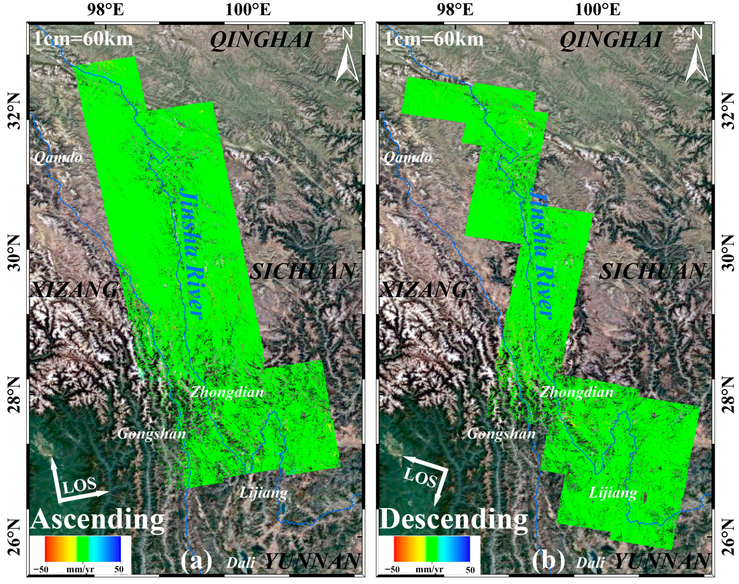
In this study (Figure 2), the Line-of-Sight (LOS) annual displacement deformation rates were obtained from the work of Zhang et al., who processed Sentinel-1 imagery (including 372 ascending and 580 descending scenes acquired between 2017 and 2020) using the Generic Atmospheric Correction Online Service (GACOS) combined with the SBAS-InSAR technique. During the processing, elevation-dependent and long-wavelength atmospheric errors in each unwrapped interferogram were mitigated using GACOS, followed by a spatio-temporal APS filter to reduce short-wavelength disturbances. The quality of phase loop closure was evaluated by calculating the RMS of the loop closure phase, with pixels exceeding 1.5 rad being excluded. Subsequently, mean LOS surface displacement rates and corresponding time series were derived through least squares estimation [38,39]. Please refer to Zhang et al. (2022) for a detailed processing procedure [12].

2.3. Landslide Dataset Construction

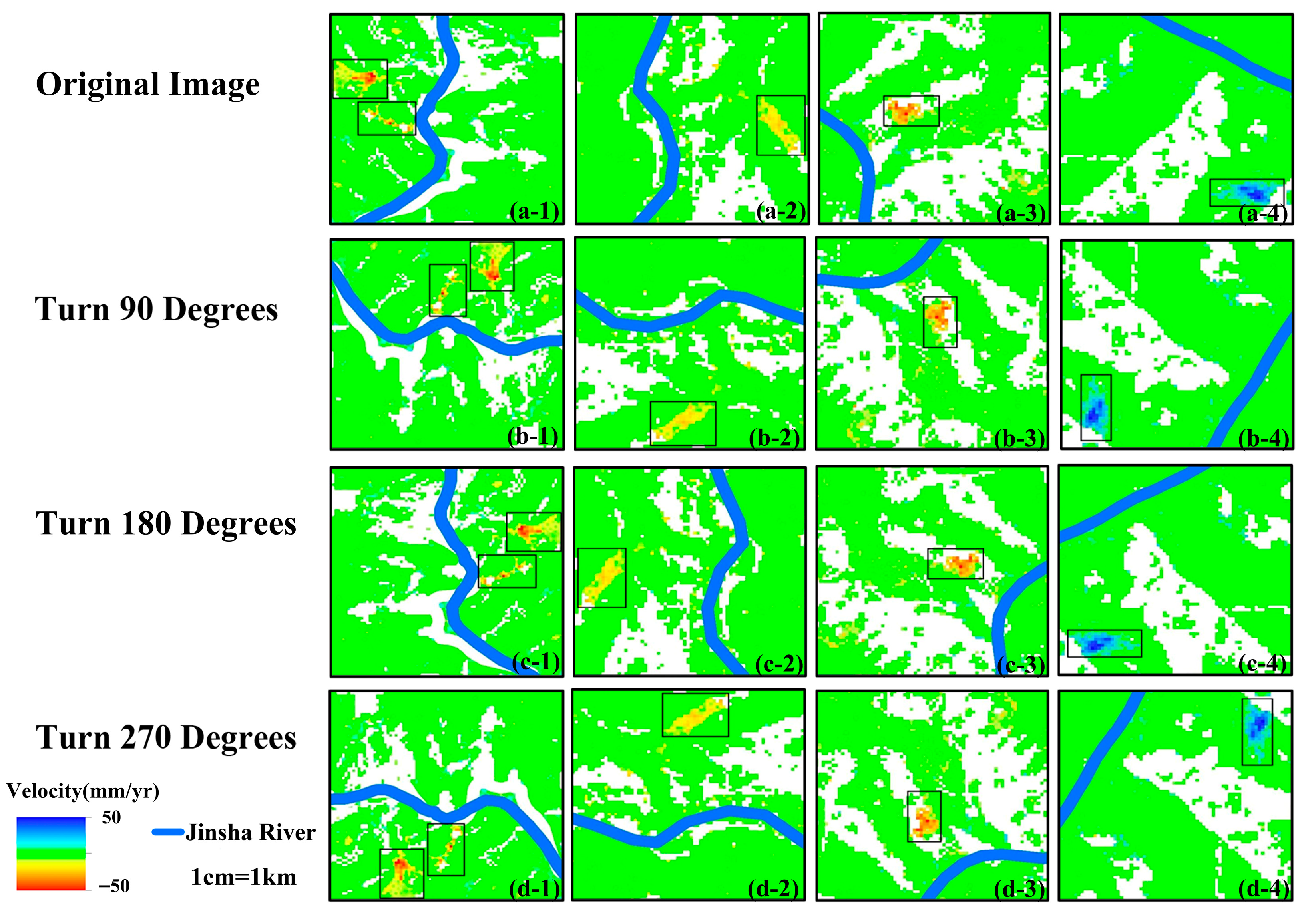
The construction of a high-quality landslide deformation rate image dataset served as a fundamental prerequisite for model training. In this study, we established a specialized landslide inventory by applying threshold criteria of InSAR deformation rates covering the upper and middle reaches of the Jinsha River Basin, as illustrated in Figure 3. Firstly, the deformation rates were cropped using a sliding window approach with a fixed stride and no overlap, producing output images sized 512 × 512 pixels. To overcome the class imbalance problem in DL [40,41], samples with deformation rates less than 10 mm/yr, as well as those located more than 50 km from the Jinsha River, were excluded from the study. Secondly, given the limited scale of the landslide image dataset constructed in this study, data augmentation was crucial for enlarging the dataset and enhancing model training performance. To mitigate the limitation of small sample size and enable the model to learn more diverse feature representations, a systematic rotational strategy was employed, rotating each sample clockwise by 90°, 180°, and 270°. This augmentation process quadrupled the dataset size from 422 to 1688 high-confidence samples. Finally, a total of 1012 samples were meticulously annotated in Pascal VOC format using the LabelImg tool. The labeled dataset was partitioned into training and validation sets at a 7:3 ratio for model development. Following initial training, the resulting model was employed to automatically identify the remaining 676 unlabeled landslide samples. To enhance training efficiency and model performance, a transfer learning approach was adopted, initializing the network with weights pre-trained on the Common Objects in Context (COCO) dataset [42].

3. Methods

3.1. Faster R-CNN Algorithm

Faster R-CNN represents a seminal two-stage object detection framework that demonstrates exceptional performance in the field of computer vision. While two-stage detectors exhibit lower computational efficiency compared to single-stage algorithms, their superior accuracy renders them particularly suitable for landslide detection studies. In 2016, Ren et al. proposed the Faster R-CNN algorithm [43,44], which incorporates a Region Proposal Network (RPN) to replace traditional sliding-window detection, thereby enhancing the speed of bounding box generation.
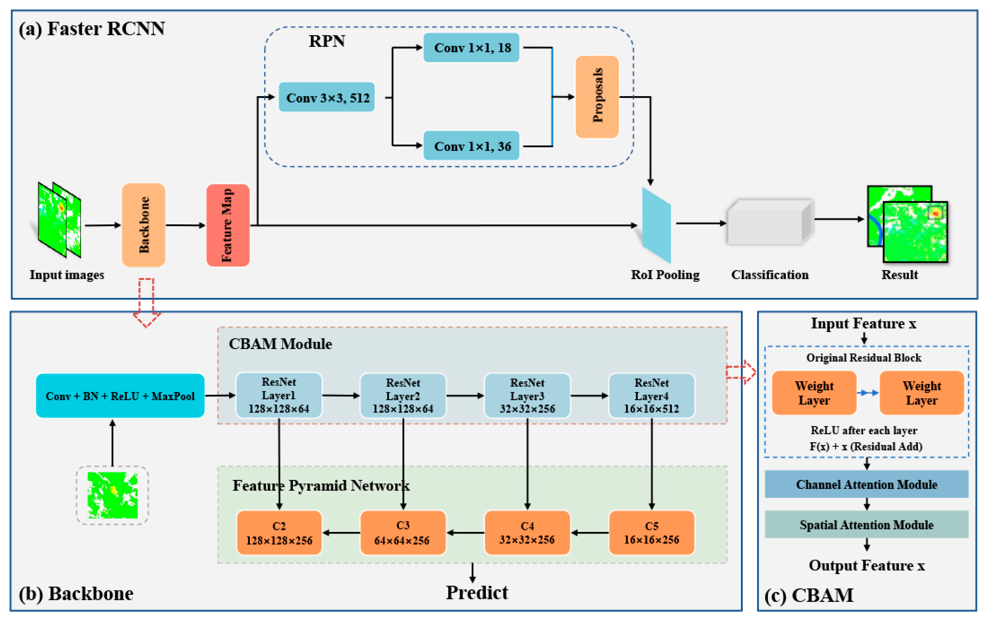
The overall architecture of Faster R-CNN, as illustrated in Figure 4a, comprises four principal modules: the backbone network, RPN, RoI Pooling (RoI), and Classification. The backbone network extracts hierarchical features from InSAR deformation rates and generates feature maps. A subset of these feature maps is processed by the RPN, which identifies potential landslide regions and proposes their approximate locations in the form of bounding boxes. Then, these proposals are passed to the RoI for further processing. The RPN is a crucial component designed to efficiently generate candidate regions likely to contain target objects. To enhance the accuracy of localization, the proposal generation process innovatively incorporates anchor boxes—predefined standard rectangular regions—which are refined through a regression module to better fit the shape and size of actual targets [45]. These serve as initial reference frames for subsequent classification and regression, generating the final proposals.
RoI plays a pivotal role in Faster R-CNN by converting the variable-sized region proposals generated by the RPN into fixed-size feature maps, thereby enabling consistent processing in the subsequent classification and bounding box regression stages. This operation addresses the issue of inconsistent input dimensions and enables the fully connected layers to uniformly process all candidate regions. The classification stage, one of the final phases in Faster R-CNN, is responsible for determining the object categories of all previously identified selected anchors based on the features extracted by RoI, while simultaneously refining their bounding boxes. This stage directly governs the detector’s accuracy and robustness.

3.2. Improved Faster R-CNN Algorithm

3.2.1. The ResNet-34 Algorithm

Deep convolutional neural networks have achieved significant advancements in image processing, substantially enhancing recognition accuracy. ResNet, a widely adopted deep convolutional neural network architecture, is constructed by stacking multiple residual blocks. This design effectively addresses the degradation problem commonly observed in deep neural networks, where increasing network depth leads to a decline in model performance, and has demonstrated strong performance across a wide range of tasks [46,47,48]. While increasing network depth can improve model performance, simply stacking additional layers typically induces two fundamental issues. Firstly, during backpropagation, gradient signals progressively diminish until approaching insignificance, a phenomenon termed the vanishing gradient problem. Second, the gradient magnitudes may grow exponentially, leading to numerical instability known as the exploding gradient problem. To address these issues, ResNet incorporates Batch Normalization (BN) layers—a technique originally proposed to stabilize training [49]—as well as residual structure. These design components mitigate gradient-related pathologies associated with conventional deep networks.
ResNet-34 employs identity mappings within its residual blocks, enabling greater network depth with fewer parameters than traditional sequential stacking, thereby enhancing overall performance. The architecture comprises five primary layers (i.e., conv1, conv2, …, conv5). The initial stage includes a 7 × 7 convolutional layer followed by a 3 × 3 max-pooling operation, both applied with a stride of 2, to rapidly reduce the spatial resolution of the feature maps. Subsequently, the residual stage comprises four residual modules (conv2 to conv5), each incorporating down sampling operations to progressively reduce feature resolution. The final layers of the network include a global average pooling (AvgPool) that replaces fully connected layers, followed by a Softmax classifier for output predictions. Further detailed parameter specifications are provided in Table 1.

3.2.2. ResNet-34 Algorithm with Integrated FPN

Traditional CNNs predominantly depend on single-scale deep features, which not only cause significant resolution degradation but also lead to inadequate detection performance for small and spatially compact landslides in InSAR deformation rate maps. To mitigate this limitation, we integrate ResNet-34 with the FPN [50]. This approach has been successfully applied in landslide detection tasks [51,52].
FPN enhances the performance of the model by assigning RoIs of different scales to the most appropriate pyramid levels, thereby improving multi-scale object detection. For an RoI with a width and height, its corresponding target pyramid level Pk is determined as shown in Equation (1). According to this assignment strategy, smaller RoI are mapped to higher-resolution feature levels, whereas larger RoI are mapped to lower-resolution feature levels, which effectively improves detection performance.
k = k 0 + l o g 2 w h 224
Among them, k is the assigned pyramid level, k0 is the reference level, and w and h are the width and height of the RoI.

3.2.3. ResNet-34 Algorithm with Integrated CBAM

InSAR deformation rate maps are often noisy and affected by decorrelation, two factors that can obscure true landslide deformation. To enhance feature discrimination, we insert the channel attention mechanism and the spatial attention mechanism after Layer 1 and Layer 2 of ResNet-34 [53], where high-resolution features (that exist in these layers) preserve fine local details. By placing CBAM in shallow layers, we enable the network to focus on subtle yet critical deformation cues, suppressing irrelevant background responses and enhancing sensitivity to slow-moving landslides [54,55].
The channel attention mechanism models the inter-dependencies among channels to highlight discriminative feature representations. Specifically, given an input feature map, AvgPool and global max pooling (MaxPool) are first applied to generate channel descriptors. These descriptors are then forwarded to a shared multi-layer perceptron (MLP) for dimensionality reduction and restoration. The outputs are aggregated via element-wise summation and activated by a sigmoid function to obtain the channel attention. The calculation process is shown in Equation (2).
M c F = σ M L P A v g P o o l F + M L P M a x P o o l F
Among them, MC is the channel attention module calculation factor, σ is sigmoid function, and F represents the feature map.
The spatial attention mechanism is complementary to channel attention and primarily focuses on determining where to emphasize within the feature map. Specifically, global average pooling and global max pooling are first applied along the channel dimension to generate two spatial descriptors. These descriptors are then concatenated and processed by a 7 × 7 convolution layer, followed by a sigmoid activation to reduce the dimension to 1channel, thereby producing the spatial attention map. The equation is shown in Equation (3).
M s F = σ f 7 × 7 A v g P o o l F ; M a x P o o l F
Among them, M s is the spatial attention module calculation factor, σ is sigmoid function, and F represents the feature map.
Overall, ResNet-34 enhances the model’s capability for deep feature extraction; FPN improves detection performance across multiple scales, particularly for small- and medium-sized landslides; CBAM strengthens the model’s focus on critical deformation regions. Together, these three components enhance the ability of the improved Faster R-CNN to effectively detect slow-moving landslides.

3.3. Hot Spot Analysis

The hot spot analysis (Getis-Ord G i * ) is a method designed to examine the correlation trends between the attribute characteristics and spatial locations of spatial data (points or regions), accurately identifying the high-cluster and low-cluster patterns in the spatial distribution of data [56,57]. This method is one of the ideal approaches for detecting landslides based on InSAR deformation rates, and the Equation is as follows:
G i d = j = 1 n w i j d x j j = 1 n x j j i
w i j d is the spatial weight matrix, which represents the spatial relationship between the currently analyzed element i and its neighboring elements j within a given distance d, x j denotes the InSAR surface deformation results; and n indicates the total number of elements.
Assuming that G i d f follows a normal distribution, the Z-score for each feature point can be calculated using Equation (5), the higher Z-score, the more pronounced the spatial clustering characteristics. In this study, the given distance d is set to 7, and regions with a Z-score greater than 2.58 (at the 99% significance level) are identified as potential landslide areas. Meanwhile, regions with a deformation rate of less than 10 mm/yr are excluded.
Z G i = G i d E G i d V a r G i d
Among them, V a r G i d represents the variance of G i d , and E G i d denotes the expected value.

3.4. K-Means Clustering

As a widely used unsupervised machine learning algorithm, the K-means algorithm has been extensively applied to clustering based on InSAR deformation rates [58,59]. It achieves classification by partitioning n observations into k clusters, where each observation belongs to the cluster corresponding to the nearest mean (cluster center), thereby minimizing the within-cluster variance, and the Equation is as follows:
m i n K = 1 K x i C k x i u k 2
u k t + 1 = 1 N k x i C k x i
K represents the cluster with similar deformation characteristics, x i denotes the deformation value of an individual measurement point, u k stands for the cluster center of K ; N k indicates the total number of measurements contained in the K cluster, and t represents the number of iterations.
Repeat the iterative process of Equations (6) and (7) until the assignment relationship between the central points and the measurement points remains stable. In this study, regions with a deformation rate of less than 10 mm/yr are excluded, and k is set to 2 according to the classification of landslide areas and non-landslide areas.

3.5. Evaluation Indices

To accurately evaluate the performance of the proposed model, precision and recall are employed as evaluation metrics [60]. Precision measures the proportion of true positive instances among all instances predicted as positive by the model, while recall reflects the proportion of actual positive instances that are correctly identified by the model. The corresponding formulas are presented in Equations (8) and (9).
P r e c i s i o n = T P T P + F P × 100 %
R e c a l l = T P T P + F N × 100 %
Among them, True Positives (TP) refers to a scenario where the model correctly identifies a positive instance of the target class, False Positives (FP) correspond to cases where the model incorrectly predicts negative instances as positive, and False Negatives (FN) denote cases where the model erroneously predicts positive instances as negative.
In practical applications, it is often necessary for a model to strike a balance between precision and recall, as relying on a single metric may not comprehensively capture the model’s overall performance. Therefore, the F1 score is introduced as the harmonic mean of these two metrics, providing a more balanced and robust evaluation index. It helps to avoid potentially misleading conclusions that may arise from using the arithmetic mean alone, as shown in Equation (10).
F 1 = 2 × P r e c i s i o n × R e c a l l P r e c i s i o n + R e c a l l
Mean average precision (mAP) is also used as the primary metric to comprehensively assess the performance of the object detection model [61]. The evaluation focuses on two Intersection over Union (IoU) thresholds: 0.5 (mAP50) and 0.5–0.95 (mAP50:95). The IoU is defined as the ratio between the area of overlap and the area of union between the detected bounding box and the ground truth bounding box, serving as a measure of the spatial agreement between them. Average Precision (AP) evaluates the trade-off between precision and recall by computing the area under the Precision-Recall (P-R) curve, which is generated by varying the confidence threshold. It reflects the model’s overall precision performance across all recall levels. The mAP is then computed as the mean of AP values across all object categories, as presented in Equations (11) and (12).
m A P = 1 N i = 1 N A P i
A P = 0 1 P r e c i s i o n R e c a l l d R e c a l l
Among them, N denotes the total number of classes, and i represents the class index. In the study, the landslide is the only class to be detected.

3.6. Experimental Environment

In this study, all DL models are implemented using the PyTorch 1.10.0 framework, with computations performed on an AutoDL cloud computing platform. The hardware configuration includes an Intel(R) Xeon(R) Platinum 8352V CPU with 55 GB memory and an NVIDIA GeForce GTX 3080Ti GPU with 12GB VRAM. Based on multiple experiments, the initial learning rate is set to 0.01 for 30 training epochs with a batch size of 4. To optimize model training, a learning rate scheduling strategy is implemented: starting from the 15th epoch, the learning rate is multiplied by 0.4 every 2 epochs.

4. Results and Discussion

4.1. Model Evaluation Results

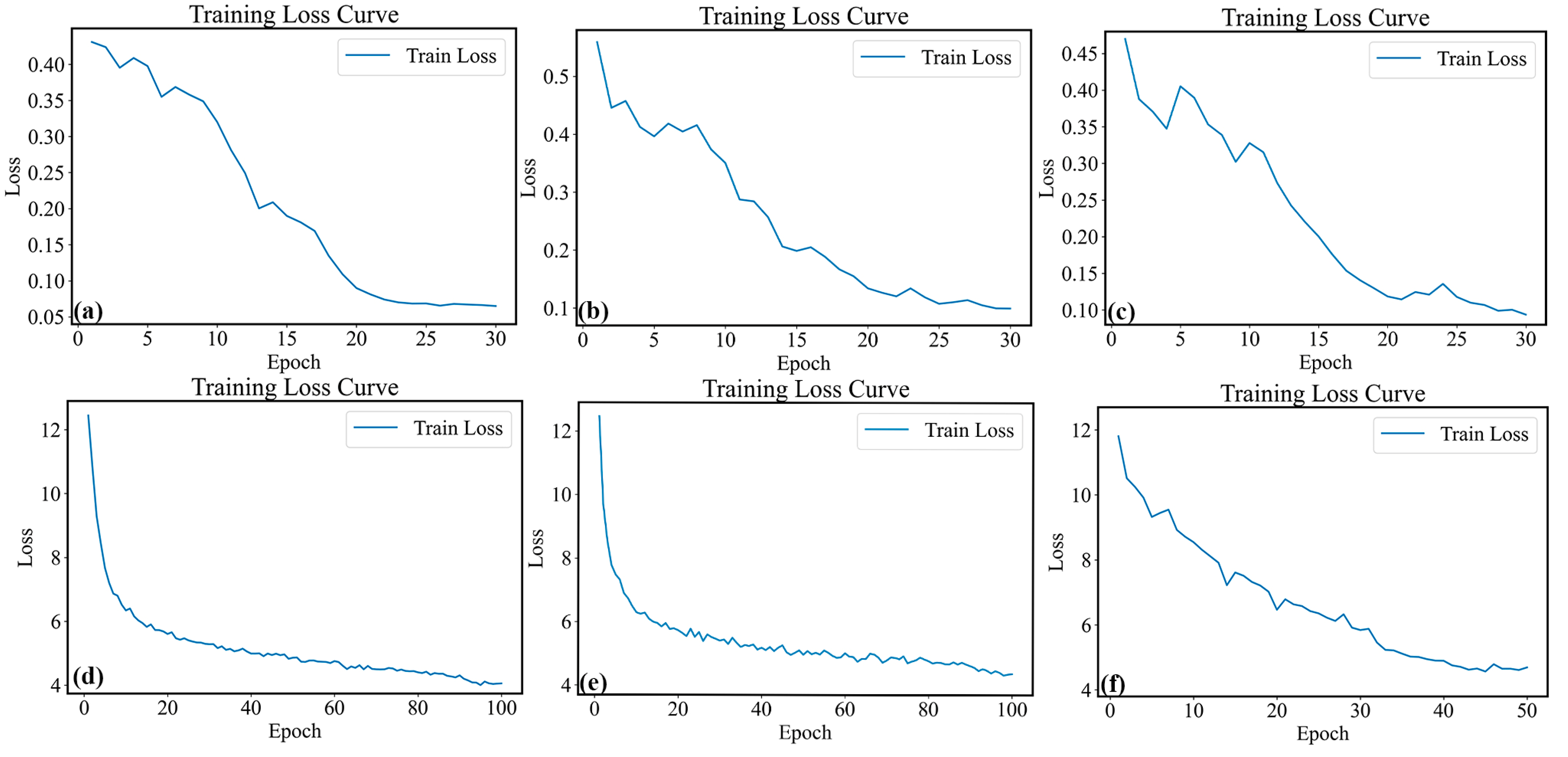
As described in Section 2.3, a landslide inventory dataset was created using the data partitioning strategy detailed above. Subsequently, we conducted performance tests on the improved algorithm and other comparative network models using this landslide dataset. Figure 5 presents the training loss curves of the six models. We can observe from Figure 5a that the decreasing trend of the loss function shifts after the 15th epoch, which is consistent with the learning rate variation we set.
As shown in Table 2, the results indicate that the improved algorithm achieved a precision of 93.56%, a recall of 97.15%, and an F1-score of 93.6% on the dataset. Compared to the latest YOLO variants and Transformer-based models (DETR), the improved model demonstrates superior performance. However, it is noteworthy that the relatively poor performance of Transformer-based models may be attributed to the limited size of the dataset, which prevented the model from fully learning the characteristics of landslide deformation. Overall, the current improved model appears to be more suitable for landslide detection. When the Intersection of Union (IoU) threshold was set to 50%, the mean Intersection of Union (mIoU) reached 93.6%, representing a 10.1% increase compared to the baseline. The experimental results show that the integration of the advanced ResNet-34 backbone with CBAM and FPN modules enables the network to focus on target-relevant regions while effectively extracting multi-scale information from InSAR deformation rate maps, thereby enhancing the model’s detection performance. The FPN primarily contributes to improved detection of small- and medium-scale landslides by retaining fine spatial details, whereas CBAM enhances sensitivity to subtle deformation features by emphasizing informative channels and spatial regions. The marked improvement in recall demonstrates that the enhanced algorithm can more effectively capture the deformation characteristics of landslides, substantially mitigating the risk of missed detections. This finding holds critical practical significance for the early identification of landslides.
To further validate the performance of the improved Faster R-CNN algorithm in detecting slow-moving landslides of varying scales, landslides have been categorized into three classes (small-scale, medium-scale, and large-scale) based on the widely adopted COCO evaluation metrics in object detection [42]. The specific classification criteria are defined as follows: landslides with an area smaller than 32 square pixels are classified as small-scale, those with 32–96 square pixels as medium-scale, and those larger than 96 square pixels as large-scale. The detection accuracy for each category of slow-moving landslides is detailed in Table 3 below.
The experimental results indicate that the model achieves optimal detection performance for large-scale landslides (area > 96 pixels2, AP = 0.693), followed by medium-scale landslides (32–96 pixels2, AP = 0.681), while it exhibits exhibiting relatively lower precision for small-scale landslides (<32 pixels2, AP = 0.591). This pattern is consistent with the role of the FPN, which enhances feature representation at multiple scales and thus benefits medium- and large-scale targets while only partly alleviating the difficulty of small-object detection. In terms of recall performance, the model demonstrates exceptional capability, achieving an overall average recall (AR) of 0.736 when the maximum number of landslide detections is set to 100. Specifically, large-scale landslides achieve the highest recall rate (AR = 0.752), followed by medium-scale landslides (AR = 0.737) and small-scale landslides (AR = 0.630). The consistently high recall across all categories further highlights the contribution of CBAM, which strengthens attention to subtle but informative deformation regions, thereby reducing the likelihood of missed detections. Further evaluation metrics reveal that the model achieves an AP@0.5 of 0.9356, an average recall rate of 0.9715, and an F1-score of 0.9360. These results robustly validate that the improved algorithm maintains high precision while maintaining outstanding recall performance. In summary, the model demonstrates robust performance in detecting slow-moving landslides across three scales, with FPN particularly improving multi-scale adaptability and CBAM ensuring sensitivity to weak deformation signals.

4.2. Slow-Moving Landslide Detection Along the Jinsha River

Based on the dataset partitioning scheme described in Section 2.3, the trained improved Faster R-CNN model was applied to slow-moving landslide detection in the upper and middle reaches of the Jinsha River Basin. The results demonstrate high confidence in detecting slow-moving landslides, indicating that the improved model exhibits strong discriminative capability and superior feature representation performance in object detection tasks.
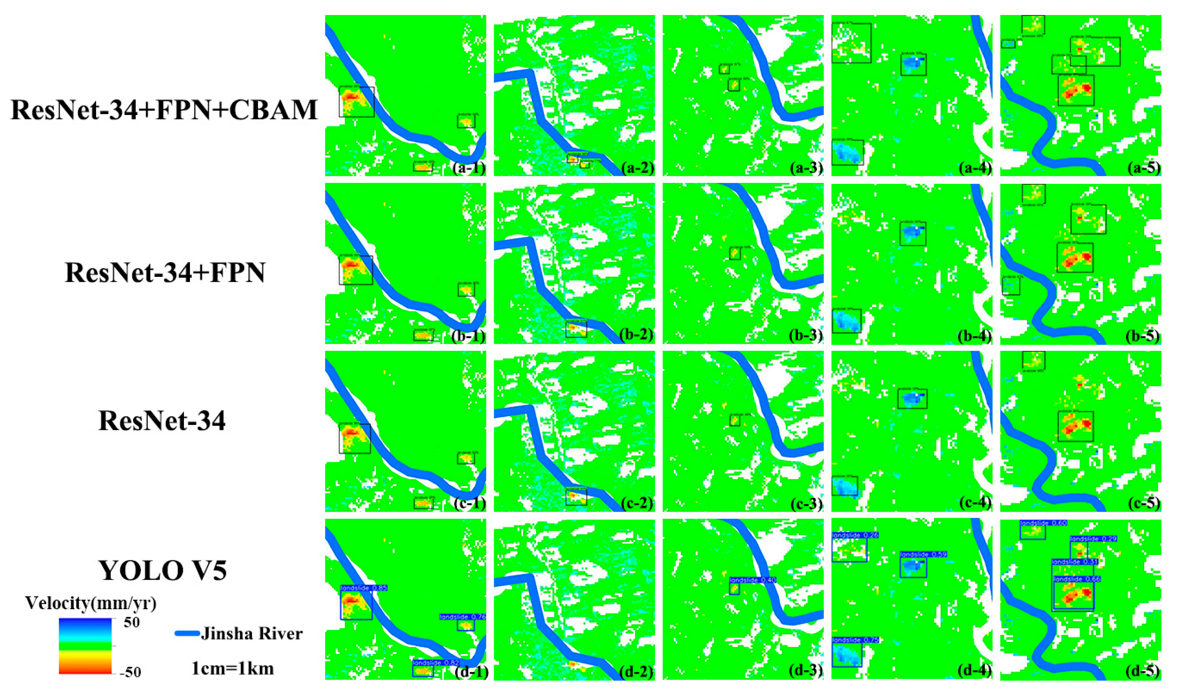
As illustrated in Figure 6, the study area is characterized by high-altitude mountainous terrain where landslide deformation information is prone to environmental interference, making it challenging to distinguish landslide deformation signals from other deformation sources (e.g., glacier movement). As shown in Figure 6(a-2,a-3), by embedding the FPN, the detection accuracy for small-area landslides is significantly improved. Meanwhile, as illustrated in Figure 6(a-5), through the integration of CBAM, the model can effectively focus on the critical deformation features of slow-moving landslides during the detection process, thereby enhancing the detection accuracy. Experimental results empirically validate the superior performance of the improved Faster R-CNN model in slow-moving landslide identification tasks, demonstrating its substantial technical advantages in complex geomorphological environments.
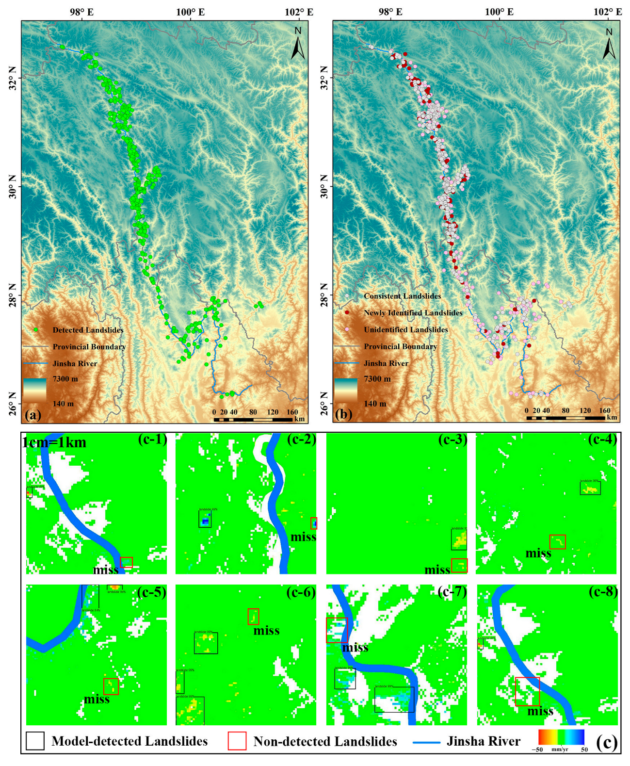
The model detected 496 slow-moving landslides in the upper and middle reaches of the Jinsha River Basin. Compared with the manual interpretation method in existing literature [12], 395 slow-moving landslides were detected, resulting in a 62.7% overlap and indicating high consistency in landslide distribution areas. Additionally, the model detected 101 new slow-moving landslides, mainly in the central region. However, the proposed model fails to detect 234 landslides, which are primarily located in the upstream and downstream regions. A possible explanation for this discrepancy is that 60 landslides were detected through SAR pixel offsets in existing literature [12], and deformation signals were not captured by InSAR. Meanwhile, in some landslide areas, the InSAR deformation rates are low and the feature of the landslide is not prominent, making it difficult for the model to accurately identify them (Figure 7(c-3–c-6)). In the downstream region, dense vegetation cover causes severe signal decorrelation, resulting in low-quality InSAR deformation data (Figure 7(c-7,c-8)). It should be noted that, although GACOS and APS were used to correct atmospheric errors, atmospheric artifacts maybe still exist due to the complex topography of the study area. However, based on the experimental results, the improved model has demonstrated the capability to effectively focus on detecting landslide deformation.

4.3. The Generalization Capability Along the Qonggyai County

To validate the regional transferability of the improved Faster R-CNN model, two representative landslide-prone areas in Qonggyai County, Shannan City, were selected. InSAR deformation rates were acquired by the GACOS-SBAS InSAR technique, and a priori landslide inventory comprising 29 landslide samples was established through the interpretation of Google Earth and Jilin-1 high-resolution optical satellite imagery, which serves as a benchmark for performance evaluation. The trained model was then applied to detect landslides within the selected areas.
Figure 8 illustrates the landslide detection results in the representative areas of Qonggyai County. A total of 39 slow-moving landslides were detected, with 27 matching existing landslide inventories and 12 newly detected landslides. The model produced confidence scores exceeding 90% for all image tiles, indicating stable detection performance in regions beyond the original training area. The remaining 3 landslides in the inventory were not successfully detected. The possible reasons are as follows: (1) the deformation rates of these landslides are extremely low, rendering their features indistinct in the deformation maps and insufficient to meet the algorithm’s detection threshold; (2) geometric distortions introduced during SAR data tiling (as illustrated in Figure 8b) caused a further reduction in the size and clarity of small landslides, leading to missed detections.
To validate the algorithm’s detection capability, hot spot analysis and K-means clustering were employed for landslide detection in the two regions, as illustrated in Figure 9. The detection results of the three methods are presented in Table 4; hot spot analysis detected 40 landslides, K-means clustering detected 34 landslides and the improved Faster R-CNN algorithm detected 38 landslides. The three methods showed a 60% overlap in detected landslides. Compared to visual interpretation results, the improved Faster R-CNN algorithm, hot spot analysis, and K-means clustering failed to identify 2, 1, and 5 landslides, respectively, while newly detected 12, 12, and 10 landslides. The improved Faster R-CNN algorithm and hot spot analysis achieve comparable accuracy and newly identified landslide counts, both out-performing K-means clustering. Unlike hot spot analysis, the trained Faster R-CNN model requires no threshold setting or parameter tuning, resulting in higher efficiency. It demonstrates balanced performance in accuracy, coverage, and novel detection. Trained solely on data from the Jinsha River Basin, the model also achieved satisfactory results in Qonggyai County without additional adjustments, indicating strong cross-regional generalization under similar geological conditions.
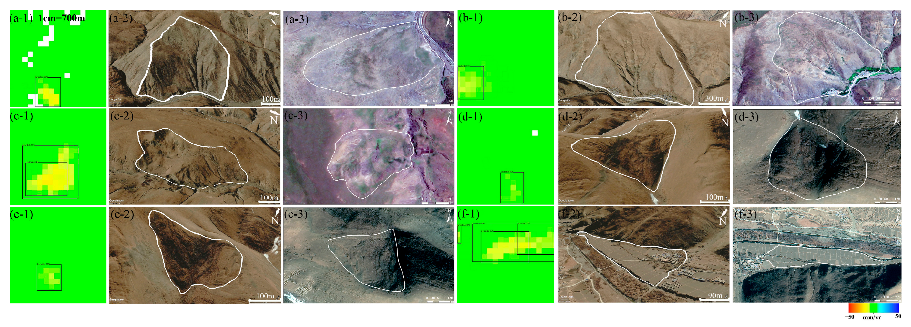
Figure 10 presents partial detection results and corresponding optical images. Figure 10(a-1–c-3) demonstrate that the proposed algorithm can effectively detect slow-moving landslides with obvious deformation (4 cm/year). Figure 10(d-1–d-3,e-1–e-3) indicate that the algorithm has a certain capability to detect landslides with indistinct displacement (2 cm/year). The landslide in Figure 10(f-1–f-3) is located at the junction of the valley bottom and the slope foot, with relatively obvious displacement. However, further judgment on whether it is a landslide should be made in combination with high spatial resolution optical images and field surveys.
It is worth noting that the present study is limited to the detection of slow-moving landslides using InSAR-derived deformation rates. Given that the study area is a high-altitude region with sparse vegetation coverage and good coherence, the deformation rate results are of high quality, which lays a solid data foundation for the intelligent extraction of slow-moving landslides. In areas with heavy vegetation coverage, however, it is impossible to comprehensively detect slow-moving landslides relying solely on single SAR data and a single InSAR technique. More importantly, identifying landslides with all velocity ranges cannot be achieved by depending exclusively on InSAR technology; instead, it requires the assistance of multiple techniques such as SAR/optical pixel offset, optical remote sensing, LiDAR, and DEM.

5. Conclusions

In this study, we propose an improved Faster R-CNN model based on InSAR deformation rates for wide-area detection of slow-moving landslides. The model was successfully applied in the middle and upper reaches of the Jinsha River Basin and further validated for generalizability in the representative landslide-prone areas of Qonggyai County.
Firstly, based on InSAR deformation rate data in the middle and upper reaches of the Jinsha River, we constructed a landslide image dataset comprising 1688 samples by data augmentation. Subsequently, the improved model was trained and tested on the dataset, successfully identifying 496 slow-moving landslides and achieving a precision of 93.56%, recall of 97.15%, F1-score of 93.60%, and mAP@50 of 93.56%. Finally, the model’s cross-regional transferability and generalization capability were evaluated in Qonggyai County, a region characterized by analogous geological conditions. The detection results demonstrated in good agreement with those derived from hotspot analysis and K-means clustering.
The findings hold substantial practical significance for disaster mitigation in the middle and upper reaches of the Jinsha River Basin. This study significantly enhances the efficiency of slow-moving landslide detection, achieving both high accuracy and detection speed. The proposed method demonstrates strong application potential in mountainous regions, providing effective support for the dynamic detection of slow-moving landslides.

Author Contributions

Conceptualization, C.Z. and J.L.; methodology, C.Z. and J.L.; formal analysis, J.L.; resources, J.L.; writing—original draft preparation, J.L.; writing—review and editing, J.L. and Z.L.; supervision, J.L. and Z.L.; funding acquisition, J.L. and Z.L. All authors have read and agreed to the published version of the manuscript.

Funding

This research is funded by the National Natural Science Foundation of China (42404020), Shaanxi Province Geoscience Big Data and Geohazard Prevention Innovation Team (2022), the Shaanxi Province Science and Technology Innovation team (Ref. 2021TD-51) and Generic Technical Development Platform of Shaanxi Province for Imaging Geodesy(2024ZG-GXPT-07). This work was also supported by the Fundamental Research Funds for the Central Universities, CHD (Ref. 300102260301, 300102261108, 300102262902, 300102264302 and 300102265103).

Data Availability Statement

Dataset available on request from the authors.

Conflicts of Interest

The authors declare no conflicts of interest.

References

  1. Guzzetti, F.; Mondini, A.C.; Cardinali, M.; Fiorucci, F.; Santangelo, M.; Chang, K.-T. Landslide inventory maps: New tools for an old problem. Earth-Sci. Rev. 2012, 112, 42–66. [Google Scholar] [CrossRef]
  2. Keefer, D.K.; Larsen, M.C. Assessing Landslide Hazards. Science 2007, 316, 1136–1138. [Google Scholar] [CrossRef]
  3. Nava, L.; Carraro, E.; Reyes-Carmona, C.; Puliero, S.; Bhuyan, K.; Rosi, A.; Monserrat, O.; Floris, M.; Meena, S.R.; Galve, J.P.; et al. Landslide displacement forecasting using deep learning and monitoring data across selected sites. Landslides 2023, 20, 2111–2129. [Google Scholar] [CrossRef]
  4. Chen, B.; Li, Z.; Zhang, C.; Ding, M.; Zhu, W.; Zhang, S.; Han, B.; Du, J.; Cao, Y.; Zhang, C.; et al. Wide Area Detection and Distribution Characteristics of Landslides along Sichuan Expressways. Remote Sens. 2022, 14, 3431. [Google Scholar] [CrossRef]
  5. Wang, H.; Zhang, L.; Yin, K.; Luo, H.; Li, J. Landslide identification using machine learning. Geosci. Front. 2021, 12, 351–364. [Google Scholar] [CrossRef]
  6. Massonnet, D.; Rossi, M.; Carmona, C.; Adragna, F.; Peltzer, G.; Feigl, K.; Rabaute, T. The displacement field of the Landers earthquake mapped by radar interferometry. Nature 1993, 364, 138–142. [Google Scholar] [CrossRef]
  7. Reale, D.; Verde, S.; Calà, F.; Imperatore, P.; Pauciullo, A.; Pepe, A.; Zamparelli, V.; Sansosti, E.; Fornaro, G. Multipass InSAR with Multiple Bands: Application to Landslides Mapping and Monitoring. In Proceedings of the IGARSS 2022—2022 IEEE International Geoscience and Remote Sensing Symposium, Kuala Lumpur, Malaysia, 17–22 July 2022; pp. 4510–4513. [Google Scholar]
  8. Bhattacharya, A.; Mukherjee, K. Review on InSAR based displacement monitoring of Indian Himalayas: Issues, challenges and possible advanced alternatives. Geocarto Int. 2017, 32, 298–321. [Google Scholar] [CrossRef]
  9. Wasowski, J.; Bovenga, F. Chapter 11—Remote sensing of landslide motion with emphasis on satellite multi-temporal interferometry applications: An overview. In Landslide Hazards, Risks, and Disasters, 2nd ed.; Davies, T., Rosser, N., Shroder, J.F., Eds.; Elsevier: Amsterdam, The Netherlands, 2022; pp. 365–438. [Google Scholar]
  10. Pedretti, L.; Bordoni, M.; Vivaldi, V.; Figini, S.; Parnigoni, M.; Grossi, A.; Lanteri, L.; Tararbra, M.; Negro, N.; Meisina, C. InterpolatiON of InSAR Time series for the dEtection of ground deforMatiOn eVEnts (ONtheMOVE): Application to slow-moving landslides. Landslides 2023, 20, 1797–1813. [Google Scholar] [CrossRef]
  11. Zhang, L.L.; Dai, K.R.; Deng, J.; Ge, D.Q.; Liang, R.B.; Li, W.L.; Xu, Q. Identifying Potential Landslides by Stacking-InSAR in Southwestern China and Its Performance Comparison with SBAS-InSAR. Remote Sens. 2021, 13, 3662. [Google Scholar] [CrossRef]
  12. Zhang, C.; Li, Z.; Yu, C.; Chen, B.; Ding, M.; Zhu, W.; Yang, J.; Liu, Z.; Peng, J. An integrated framework for wide-area active landslide detection with InSAR observations and SAR pixel offsets. Landslides 2022, 19, 2905–2923. [Google Scholar] [CrossRef]
  13. Yazici, B.V.; Gormus, E.T. Investigating persistent scatterer InSAR (PSInSAR) technique efficiency for landslides mapping: A case study in Artvin dam area, in Turkey. Geocarto Int. 2022, 37, 2293–2311. [Google Scholar] [CrossRef]
  14. Wang, G.J.; Xie, M.W.; Chai, X.Q.; Wang, L.W.; Dong, C.X. D-InSAR-based landslide location and monitoring at Wudongde hydropower reservoir in China. Environ. Earth Sci. 2013, 69, 2763–2777. [Google Scholar] [CrossRef]
  15. Solari, L.; Del Soldato, M.; Raspini, F.; Barra, A.; Bianchini, S.; Confuorto, P.; Casagli, N.; Crosetto, M. Review of Satellite Interferometry for Landslide Detection in Italy. Remote Sens. 2020, 12, 1351. [Google Scholar] [CrossRef]
  16. Liu, X.; Zhao, C.; Zhang, Q.; Lu, Z.; Li, Z.; Yang, C.; Zhu, W.; Liu-Zeng, J.; Chen, L.; Liu, C. Integration of Sentinel-1 and ALOS/PALSAR-2 SAR datasets for mapping active landslides along the Jinsha River corridor, China. Eng. Geol. 2021, 284, 106033. [Google Scholar] [CrossRef]
  17. Di Martire, D.; Paci, M.; Confuorto, P.; Costabile, S.; Guastaferro, F.; Verta, A.; Calcaterra, D. A nation-wide system for landslide mapping and risk management in Italy: The second Not-ordinary Plan of Environmental Remote Sensing. Int. J. Appl. Earth Obs. Geoinf. 2017, 63, 143–157. [Google Scholar] [CrossRef]
  18. Tomás, R.; Pagán, J.I.; Navarro, J.A.; Cano, M.; Pastor, J.L.; Riquelme, A.; Cuevas-González, M.; Crosetto, M.; Barra, A.; Monserrat, O.; et al. Semi-Automatic Identification and Pre-Screening of Geological–Geotechnical Deformational Processes Using Persistent Scatterer Interferometry Datasets. Remote Sens. 2019, 11, 1675. [Google Scholar] [CrossRef]
  19. He, Y.; Wenhui, W.; Lifeng, Z.; Youdong, C.; Yi, C.; Baoshan, C.; Xu, H.; Zhao, Z. An identification method of potential landslide zones using InSAR data and landslide susceptibility. Geomat. Nat. Hazards Risk 2023, 14, 2185120. [Google Scholar] [CrossRef]
  20. Wang, Y.; Dong, J.; Zhang, L.; Deng, S.; Zhang, G.; Liao, M.; Gong, J. Automatic detection and update of landslide inventory before and after impoundments at the Lianghekou reservoir using Sentinel-1 InSAR. Int. J. Appl. Earth Obs. Geoinf. 2023, 118, 103224. [Google Scholar] [CrossRef]
  21. Lu, P.; Bai, S.; Tofani, V.; Casagli, N. Landslides detection through optimized hot spot analysis on persistent scatterers and distributed scatterers. ISPRS J. Photogramm. Remote Sens. 2019, 156, 147–159. [Google Scholar] [CrossRef]
  22. Han, J.; Guo, X.; Jiao, R.; Nan, Y.; Yang, H.; Ni, X.; Zhao, D.; Wang, S.; Ma, X.; Yan, C.; et al. An Automatic Method for Delimiting Deformation Area in InSAR Based on HNSW-DBSCAN Clustering Algorithm. Remote Sens. 2023, 15, 4287. [Google Scholar] [CrossRef]
  23. Ding, A.; Zhang, Q.; Zhou, X.; Dai, B. Automatic recognition of landslide based on CNN and texture change detection. In Proceedings of the 2016 31st Youth Academic Annual Conference of Chinese Association of Automation (YAC), Wuhan, China, 11–13 November 2016; pp. 444–448. [Google Scholar]
  24. Yu, H.; Ma, Y.; Wang, L.; Zhai, Y.; Wang, X. A landslide intelligent detection method based on CNN and RSG_R. In Proceedings of the 2017 IEEE International Conference on Mechatronics and Automation (ICMA), 6–9 August 2017; pp. 40–44. [Google Scholar]
  25. Ghorbanzadeh, O.; Blaschke, T.; Gholamnia, K.; Meena, S.R.; Tiede, D.; Aryal, J. Evaluation of Different Machine Learning Methods and Deep-Learning Convolutional Neural Networks for Landslide Detection. Remote Sens. 2019, 11, 196. [Google Scholar] [CrossRef]
  26. Jiang, W.; Xi, J.; Li, Z.; Zang, M.; Chen, B.; Zhang, C.; Liu, Z.; Gao, S.; Zhu, W. Deep Learning for Landslide Detection and Segmentation in High-Resolution Optical Images along the Sichuan-Tibet Transportation Corridor. Remote Sens. 2022, 14, 5490. [Google Scholar] [CrossRef]
  27. Anantrasirichai, N.; Biggs, J.; Albino, F.; Hill, P.; Bull, D. Application of Machine Learning to Classification of Volcanic Deformation in Routinely Generated InSAR Data. J. Geophys. Res. Solid Earth 2018, 123, 6592–6606. [Google Scholar] [CrossRef]
  28. Brengman, C.M.J.; Barnhart, W.D. Identification of Surface Deformation in InSAR Using Machine Learning. Geochem. Geophys. Geosyst. 2021, 22, e2020GC009204. [Google Scholar] [CrossRef]
  29. Wu, Z.P.; Wang, T.; Wang, Y.J.; Wang, R.; Ge, D.Q. Deep Learning for the Detection and Phase Unwrapping of Mining-Induced Deformation in Large-Scale Interferograms. IEEE Trans. Geosci. Remote Sens. 2022, 60, 5216318. [Google Scholar] [CrossRef]
  30. Zhao, Y.; Feng, G.; Wang, Y.; Wang, X.; Wang, Y.; Lu, H.; Xu, W.; Wang, H. A new algorithm for intelligent detection of geohazards incorporating attention mechanism. Int. J. Appl. Earth Obs. Geoinf. 2022, 113, 102988. [Google Scholar] [CrossRef]
  31. Ma, R.P.; Yu, H.Y.; Liu, X.J.; Yuan, X.R.; Geng, T.T.; Li, P.A. InSAR-YOLOv8 for wide-area landslide detection in InSAR measurements. Sci. Rep. 2025, 15, 1595. [Google Scholar] [CrossRef] [PubMed]
  32. Yong, L.; Xiaoyi, F.; Genwei, C. Landslide and rockfall distribution by reservior of stepped hydropower station in the Jinsha River. Wuhan Univ. J. Nat. Sci. 2006, 11, 801–805. [Google Scholar] [CrossRef]
  33. Fan, X.; Xu, Q.; Alonso-Rodriguez, A.; Subramanian, S.S.; Li, W.; Zheng, G.; Dong, X.; Huang, R. Successive landsliding and damming of the Jinsha River in eastern Tibet, China: Prime investigation, early warning, and emergency response. Landslides 2019, 16, 1003–1020. [Google Scholar] [CrossRef]
  34. Ran, Y.; Li, X.; Cheng, G.; Zhang, T.; Wu, Q.; Jin, H.; Jin, R. Distribution of Permafrost in China: An Overview of Existing Permafrost Maps. Permafr. Periglac. Process. 2012, 23, 322–333. [Google Scholar] [CrossRef]
  35. Liu, H.; Lan, H.; Liu, Y.; Zhou, Y. Characteristics of spatial distribution of debris flow and the effect of their sediment yield in main downstream of Jinsha River, China. Environ. Earth Sci. 2011, 64, 1653–1666. [Google Scholar] [CrossRef]
  36. Zhou, J.-W.; Xu, W.; Yang, X.-G.; Shi, C.; Yang, Z. The 28 October 1996 landslide and analysis of the stability of the current Huashiban slope at the Liangjiaren Hydropower Station, Southwest China. Eng. Geol. 2010, 114, 45–56. [Google Scholar] [CrossRef]
  37. Zhao, W.; Wang, F.; Xu, Q.; Zhao, J.; Zhang, F.; Li, W.; Dong, X.; Yang, J.; Guo, D.; He, W. Identification, distribution, and mechanisms of large landslides in the upper reaches of Jinsha River. Bull. Eng. Geol. Environ. 2025, 84, 199. [Google Scholar] [CrossRef]
  38. Yu, C.; Li, Z.; Penna, N.T. Triggered afterslip on the southern Hikurangi subduction interface following the 2016 Kaikōura earthquake from InSAR time series with atmospheric corrections. Remote Sens. Environ. 2020, 251, 112097. [Google Scholar] [CrossRef]
  39. Li, Z.; Fielding, E.J.; Cross, P. Integration of InSAR Time-Series Analysis and Water-Vapor Correction for Mapping Postseismic Motion After the 2003 Bam (Iran) Earthquake. IEEE Trans. Geosci. Remote Sens. 2009, 47, 3220–3230. [Google Scholar] [CrossRef]
  40. Jing, X.Y.; Zhang, X.; Zhu, X.; Wu, F.; You, X.; Gao, Y.; Shan, S.; Yang, J.Y. Multiset Feature Learning for Highly Imbalanced Data Classification. IEEE Trans. Pattern Anal. Mach. Intell. 2021, 43, 139–156. [Google Scholar] [CrossRef]
  41. Fernández, A.; García, S.; del Jesus, M.J.; Herrera, F. A study of the behaviour of linguistic fuzzy rule based classification systems in the framework of imbalanced data-sets. Fuzzy Sets Syst. 2008, 159, 2378–2398. [Google Scholar] [CrossRef]
  42. Lin, T.-Y.; Maire, M.; Belongie, S.; Hays, J.; Perona, P.; Ramanan, D.; Dollár, P.; Zitnick, C.L. Microsoft COCO: Common Objects in Context. In Proceedings of the Computer Vision—ECCV 2014, Zurich, Switzerland, 6–12 September 2014; pp. 740–755. [Google Scholar]
  43. Girshick, R. Fast R-CNN. In Proceedings of the 2015 IEEE International Conference on Computer Vision (ICCV), Santiago, Chile, 7–13 December 2015; pp. 1440–1448. [Google Scholar]
  44. Ren, S.; He, K.; Girshick, R.; Sun, J. Faster R-CNN: Towards Real-Time Object Detection with Region Proposal Networks. IEEE Trans. Pattern Anal. Mach. Intell. 2017, 39, 1137–1149. [Google Scholar] [CrossRef] [PubMed]
  45. Vo, X.T.; Jo, K.H. A review on anchor assignment and sampling heuristics in deep learning-based object detection. Neurocomputing 2022, 506, 96–116. [Google Scholar] [CrossRef]
  46. He, K.; Zhang, X.; Ren, S.; Sun, J. Deep Residual Learning for Image Recognition. In Proceedings of the 2016 IEEE Conference on Computer Vision and Pattern Recognition (CVPR), Las Vegas, NV, USA, 27–30 June 2016; pp. 770–778. [Google Scholar]
  47. Roy, S.K.; Manna, S.; Song, T.C.; Bruzzone, L. Attention-Based Adaptive SpectralSpatial Kernel ResNet for Hyperspectral Image Classification. IEEE Trans. Geosci. Remote Sens. 2021, 59, 7831–7843. [Google Scholar] [CrossRef]
  48. Haut, J.M.; Paoletti, M.E.; Plaza, J.; Plaza, A.; Li, J. Visual Attention-Driven Hyperspectral Image Classification. IEEE Trans. Geosci. Remote Sens. 2019, 57, 8065–8080. [Google Scholar] [CrossRef]
  49. Ioffe, S.; Szegedy, C. Batch normalization: Accelerating deep network training by reducing internal covariate shift. In Proceedings of the 32nd International Conference on International Conference on Machine Learning, Lille, France, 6–11 July 2015; Volume 37, pp. 448–456. [Google Scholar]
  50. Lin, T.Y.; Dollár, P.; Girshick, R.; He, K.; Hariharan, B.; Belongie, S. Feature Pyramid Networks for Object Detection. In Proceedings of the 2017 IEEE Conference on Computer Vision and Pattern Recognition (CVPR), Honolulu, HI, USA, 21–26 July 2017; pp. 936–944. [Google Scholar]
  51. Yun, L.; Zhang, X.; Zheng, Y.; Wang, D.; Hua, L. Enhance the Accuracy of Landslide Detection in UAV Images Using an Improved Mask R-CNN Model: A Case Study of Sanming, China. Sensors 2023, 23, 4287. [Google Scholar] [CrossRef]
  52. Wang, Z.; Sun, T.; Hu, K.; Zhang, Y.; Yu, X.; Li, Y. A Deep Learning Semantic Segmentation Method for Landslide Scene Based on Transformer Architecture. Sustainability 2022, 14, 16311. [Google Scholar] [CrossRef]
  53. Woo, S.; Park, J.; Lee, J.-Y.; Kweon, I.S. CBAM: Convolutional Block Attention Module. In Proceedings of the Computer Vision—ECCV 2018, Munich, Germany, 8–14 September 2018; pp. 3–19. [Google Scholar]
  54. Chandra, N.; Vaidya, H.; Sawant, S.; Meena, S.R. A Novel Attention-Based Generalized Efficient Layer Aggregation Network for Landslide Detection from Satellite Data in the Higher Himalayas, Nepal. Remote Sens. 2024, 16, 2598. [Google Scholar] [CrossRef]
  55. Meng, S.; Shi, Z.; Pirasteh, S.; Ullo, S.L.; Peng, M.; Zhou, C.; Gonçalves, W.N.; Zhang, L. TLSTMF-YOLO: Transfer Learning and Feature Fusion Network for Earthquake-Induced Landslide Detection in Remote Sensing Images. IEEE Trans. Geosci. Remote Sens. 2025, 63, 1–12. [Google Scholar] [CrossRef]
  56. Liang, Y.; Zhang, Y.; Li, Y.; Xiong, J. Automatic Identification for the Boundaries of InSAR Anomalous Deformation Areas Based on Semantic Segmentation Model. Remote Sens. 2023, 15, 5262. [Google Scholar] [CrossRef]
  57. Zhang, J.; Zhu, W.; Cheng, Y.; Li, Z. Landslide Detection in the Linzhi–Ya’an Section along the Sichuan–Tibet Railway Based on InSAR and Hot Spot Analysis Methods. Remote Sens. 2021, 13, 3566. [Google Scholar] [CrossRef]
  58. Chong, Y.; Zeng, Q. Long-Term Ground Deformation Monitoring and Quantitative Interpretation in Shanghai Using Multi-Platform TS-InSAR, PCA, and K-Means Clustering. Remote Sens. 2024, 16, 4188. [Google Scholar] [CrossRef]
  59. Festa, D.; Novellino, A.; Hussain, E.; Bateson, L.; Casagli, N.; Confuorto, P.; Del Soldato, M.; Raspini, F. Unsupervised detection of InSAR time series patterns based on PCA and K-means clustering. Int. J. Appl. Earth Obs. Geoinf. 2023, 118, 103276. [Google Scholar] [CrossRef]
  60. Talaei Khoei, T.; Ould Slimane, H.; Kaabouch, N. Deep learning: Systematic review, models, challenges, and research directions. Neural Comput. Appl. 2023, 35, 23103–23124. [Google Scholar] [CrossRef]
  61. Everingham, M.; Van Gool, L.; Williams, C.K.I.; Winn, J.; Zisserman, A. The Pascal Visual Object Classes (VOC) Challenge. Int. J. Comput. Vis. 2010, 88, 303–338. [Google Scholar] [CrossRef]
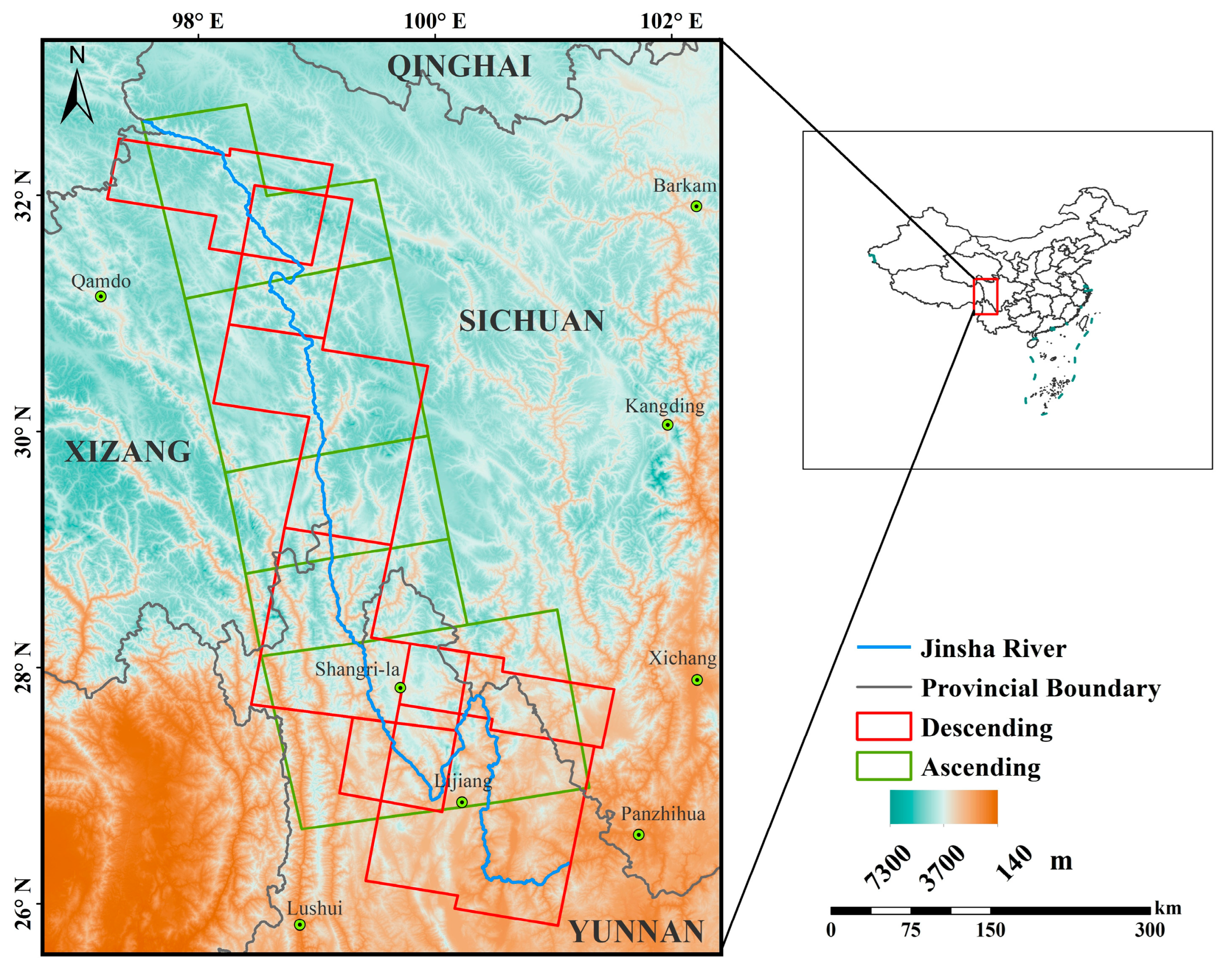
Figure 1. Overview of the study area and coverage of SAR imagery. The green line rectangles indicate the coverage of Sentinel-1 ascending images, while the red line rectangle marks the coverage of Sentinel-1 descending images. The blue and black lines are rivers and provincial boundaries, respectively.
Remotesensing 17 03243 g001
Figure 2. InSAR deformation rates in the middle and upper reaches of the Jinsha River. (a) The mean LOS surface displacement rates from Sentinel-1 ascending images, (b) The mean LOS surface displacement rates from Sentinel-1 descending images. A Positive value (blue) represents the Earth’s surface moving toward the radar, while negative values (red) indicate movement away from the radar.
Remotesensing 17 03243 g002
Figure 3. Training and landslide sample detection results based on InSAR annual displacement rate maps. (a-1d-4) represent the original data, 90 degrees rotation, 180 degrees rotation and 270 degrees rotation, respectively.
Remotesensing 17 03243 g003
Figure 4. Improved Faster R-CNN algorithm. (a) The overall architecture of Faster R-CNN; (b) backbone network composed of attention-enhanced ResNet-34 and FPN; (c) CBAM.
Remotesensing 17 03243 g004
Figure 5. The training loss curve of the four models. (a) the improved Faster R-CNN model; (b) the Faster R-CNN model with ResNet-34 and FPN; (c) the Faster R-CNN model with ResNet-34; (d) YOLO V5 model; (e) YOLO V12 model; (f) DETR model.
Remotesensing 17 03243 g005
Figure 6. Landslide detection results of different models. (a-1a-5) the Faster R-CNN with ResNet-34 +FPN+CBAM; (b-1b-5) the Faster R-CNN with ResNet-34 +FPN; (c-1c-5) the Faster R-CNN with ResNet-34; (d-1d-5) the YOLO V5 model.
Remotesensing 17 03243 g006
Figure 7. Distribution of slow-moving landslides in the Jinsha River Basin. (a) Landslide detection results using the improved Faster R-CNN algorithm; (b) Comparison with manually interpreted results from literature [12], white indicates consistent landslides; red denotes newly detected landslides by the model; pink marks those missed by the model; (c-1c-8) Results of landslides detected and undetected by the model, black boxes represent landslides detected by the model, red boxes represent the missed landslides.
Remotesensing 17 03243 g007
Figure 8. Deformation rates and slow-moving landslide detection results for two representative areas in Qonggyai County. (a,b) illustrate landslide boundaries delineated through visual interpretation (shown as red polygons) alongside the detection outputs of the trained Faster R-CNN model (black rectangles); (c) displays the recognition labels generated by the improved Faster R-CNN.
Remotesensing 17 03243 g008
Figure 9. Landslide detection results by hot spot analysis and K-means clustering. (a,b): hot spot analysis, (c,d): K-means clustering.
Remotesensing 17 03243 g009
Figure 10. Landslide deformation rates and their corresponding optical images. (a-1f-1) The landslide detection results by the improved Faster R-CNN; (a-2f-2) The landslide boundaries are derived from Google Earth; (a-3f-3) The landslide boundaries are derived from Jilin 1 optical with the images acquired in November 2021 and July 2022 at a spatial resolution of 1 m.
Remotesensing 17 03243 g010
Table 1. The ResNet-34 network structure.
Layer NameLayer StructureOutput Size
Conv17 × 7, 64, stride 2112 × 112
Conv2_x3 × 3 max pool, stride 2
3 × 3 , 64 3 × 3 , 64 × 3
56 × 56
Conv3_x 3 × 3 , 128 3 × 3 , 128 × 428 × 28
Conv4_x 3 × 3 , 256 3 × 3 , 256 × 614 × 14
Conv5_x 3 × 3 , 512 3 × 3 , 512 × 37 × 7
1 × 1Avgpool, SoftMax
Table 2. Performance comparison of improved Faster R-CNN and other models on the dataset.
MethodBackbonePrecisionRecallF1mAP 50mAP 50-95
Faster R-CNNResNet-34+FPN+CBAM93.56%97.15%93.60%93.56%67.80%
Faster R-CNNResNet-34+FPN86.67%81.94%84.24%86.70%61.30%
Faster R-CNNResNet-3483.30%76.02%79.48%83.50%42.80%
YOLO V5Darknet5383.18%79.52%81.30%85.27%52.47%
YOLO V12R-ELAN86.06%83.19%84.56%87.20%58.39%
DETRResNet-5079.56%81.34%80.42%82.31%45.96%
Table 3. Evaluation Results Based on COCO Metrics.
MetricIoU ThresholdArea CategorymaxDetsValue
Average Precision (AP)0.50:0.95all1000.678
Average Precision (AP)0.50all1000.936
Average Precision (AP)0.75all1000.797
Average Precision (AP)0.50:0.95small1000.591
Average Precision (AP)0.50:0.95medium1000.681
Average Precision (AP)0.50:0.95large1000.693
Average Recall (AR)0.50:0.95all10.328
Average Recall (AR)0.50:0.95all100.735
Average Recall (AR)0.50:0.95all1000.736
Average Recall (AR)0.50:0.95small1000.630
Average Recall (AR)0.50:0.95medium1000.737
Average Recall (AR)0.50:0.95medium1000.752
Table 4. Detection results of the three methods compared with visual interpretation.
MethodCorrectly DetectedNot DetectedNewly DetectedTotal Detected
Improved Faster R-CNN2721239
Hot Spot Analysis2811240
K-Means Clustering2451034
Disclaimer/Publisher’s Note: The statements, opinions and data contained in all publications are solely those of the individual author(s) and contributor(s) and not of MDPI and/or the editor(s). MDPI and/or the editor(s) disclaim responsibility for any injury to people or property resulting from any ideas, methods, instructions or products referred to in the content.