Article

Hierarchical Frequency-Guided Knowledge Reconstruction for SAR Incremental Target Detection

1
School of Information and Communication Engineering, University of Electronic Science and Technology of China, Chengdu 610299, China
2
Intelligent Terminal Key Laboratory of Sichuan Province, Yibin 644000, China
*
Author to whom correspondence should be addressed.
Remote Sens. 2025, 17(18), 3214; https://doi.org/10.3390/rs17183214
Submission received: 11 August 2025 / Revised: 9 September 2025 / Accepted: 15 September 2025 / Published: 17 September 2025

Abstract

Highlights

What are the main findings?
  • We tackle feature representation mismatches in SAR incremental target detection.
  • We propose HFKR, a wavelet-guided hierarchical frequency reconstruction method.
What is the implication of the main finding?
  • HFKR delivers top performance and stable learning across scenes and multi-step runs.
  • HFKR is designed as an independent modular component, which makes it potentially applicable to other domains.

Abstract

Synthetic Aperture Radar (SAR) incremental target detection faces challenges from the limits of incremental learning frameworks and distinctive properties of SAR imagery. The limited spatial representation of targets, combined with strong background interference and fluctuating scattering characteristics, leads to unstable feature learning when new classes are introduced. These factors exacerbate representation mismatches between existing and incremental tasks, resulting in significant degradation in detection performance. To address these challenges, we propose a novel incremental learning framework featuring Hierarchical Frequency-Knowledge Reconstruction (HFKR). HFKR leverages wavelet-based frequency decomposition and cross-domain feature reconstruction to enhance consistency between global and detailed features throughout the incremental learning process. Specifically, we analyze the manifestation of representation mismatch in feature space and its impact on detection accuracy, while investigating the correlation between hierarchical semantic features and frequency-domain components. Based on these insights, HFKR is embedded within the feature transfer phase, where frequency-guided decomposition and reconstruction facilitate seamless integration of new and old task features, thereby maintaining model stability across updates. Extensive experiments on two benchmark SAR datasets, MSAR and SARAIRcraft, demonstrate that our method delivers superior performance compared to existing incremental detection approaches. Furthermore, its robustness in multi-step incremental scenarios highlights the potential of HFKR for broader applications in SAR image analysis.

1. Introduction

Owing to its distinctive capabilities of all-weather operability, penetration robustness, and persistent observational continuity, Synthetic Aperture Radar (SAR) exhibits indispensable utility in critical domains including oceanic surveillance, geohazard mitigation, and urban spatial planning. As a fundamental task in SAR image interpretation, target detection focuses on achieving precise target localization within complex scenes, serving as a pivotal technological enabler for both military reconnaissance systems and civilian infrastructure management platforms. Traditional methods predominantly rely on manually engineered features and statistical models [1,2], exemplified by the Constant False Alarm Rate (CFAR) detection framework [3] and attribute scattering center models. Nevertheless, these approaches demonstrate inadequate representational capacity for intricate scattering patterns and morphological diversity inherent in high-resolution SAR imagery, while their performance susceptible to degradation under complex scene interference and operational condition variations.
In recent years, deep learning techniques have substantially enhanced the accuracy and generalization of SAR target detection through end-to-end feature learning mechanisms. Detection frameworks based on convolutional neural network (CNN) [4,5,6,7], multi-scale fusion methods driven by the attention mechanism [8,9], and enhancement methods combined with polarization information [10,11,12,13,14,15] have gradually become the mainstream of SAR target detection methods.
Despite the superior performance of deep learning methods, they are highly dependent on large-scale labeled data, which becomes a bottleneck for practical applications. SAR image labeling requires specialized domain knowledge and is much more difficult to obtain than optical images due to imaging costs and confidentiality [16]. In addition, with the dynamic expansion of targets in real-world scenarios (e.g., the emergence of new targets, new scenes, and new sensors), static detection models confront a “catastrophic forgetting” problem [17,18,19], making it difficult to learn new categories of knowledge while maintaining the old target detection capability.
Against this background, the incremental learning (IL) approach provides new ideas for model updating in data-constrained scenarios. Incremental learning can refresh the model without using old data or with a minimal amount of old data, which can effectively alleviate catastrophic forgetting while avoiding repeated training. Due to its practicality, many deep learning-based target detection methods have been extended from offline learning to incremental learning. Incremental learning was initially applied to target classification, with representative works including iCaRL [20] based on replay mechanism and LwF based on regression. Fast-ILOD [21] was the first to introduce incremental learning to target detection, utilizing knowledge distillation (KD) and parameter isolation to migrate LwF to Fast-RCNN [22]. Despite its limited utility due to the use of a non-end-to-end detector, this work offers a viable paradigm for incremental target detection methods. Subsequent works such as Faster-RCNN [23], SID [24], and ERD [25] have employed incremental learning frameworks based on KD. Although there are also works on giving replay and meta-learning, KD based methods are still mainstream.
The above methods are mostly designed for optical images and do not fully consider the unique characteristics of SAR images. The core of an ideal incremental learning method lies in stability and adaptability: expanding detailed features adaptively while maintaining the stability of underlying features (generic features) [26,27]. The rich semantic information and quantitative scale of optical datasets (e.g., COCO [28], VOC [29], etc.) endow the model with stable feature representations, and thus prior approaches have focused on maintaining balancing new and old knowledge within the model. But the sparse feature distribution and high-frequency sensitivity of SAR images cause the feature space to be prone to irreversible distortion during the incremental learning process [30]. As illustrated in Figure 1, the original model, M o r i , is trained using ship and bridge data, while M i n c is trained incrementally based on M o r i with additional oilcan and airplane data. From the feature maps spanning layers p 0 to p 3 , a noticeable shift is observed in M i n c ’s shallow features ( p 0 and p 1 ). Specifically, p 1 exhibits increased attention to near-shore land regions in the upper-left corner, which are irrelevant to the target objects. More critically, M i n c ’s deep features fail to capture key semantic regions, indicating that the original coupling strategy between global and detailed features has broken down. This degradation ultimately leads to misclassification and false alarms, as shown in the detection result Figure 1. In this study, we define this phenomenon as feature representation mismatch [31,32].
Inspired by the multi-scale property of wavelet transform, this paper addresses the feature representation mismatch problem in SAR incremental target detection by strengthening the correlation between global and detailed features. Initially, we analyze the process of model cascading hierarchical features and experimentally verify the correlation between frequency domain features and hierarchical features, establishing a frequency domain-hierarchical feature correlation model. Subsequently, we design the Hierarchical Frequency-Knowledge Reconstruction (HFKR) for SAR incremental target detection. The HFKR is applied in the feature transfer stage of model training, strengthening the correlation between underlying features and detailed features while protecting the model’s underlying knowledge memory through wavelet decomposition, cross-fertilization, and feature remodeling of the teacher and student model features.
In the subsequent part of this paper, Section 2 summarizes previous relevant work. Section 3 details the implementation of our method. Section 4 validates our method’s effectiveness using the MSAR [33] and SARAIRcraft [34] datasets. The key contributions of this paper are as follows:
1.
We analyze the impact of sparse target feature distribution and sensitivity to environmental variations in SAR imagery on incremental target detection, highlighting feature representation mismatch as a key factor driving performance degradation across incremental tasks.
2.
We conduct a comprehensive analysis of the correlation between frequency-domain components and hierarchical semantic features in SAR imagery. This analysis demonstrates that frequency-domain representations more clearly capture multi-scale semantic structures, providing essential guidance for the design of our subsequent reconstruction strategy.
3.
Building upon above analysis, we design the HFKR strategy, which integrates frequency-guided decomposition and reconstruction into the feature transfer process. HFKR effectively addresses feature representation mismatch challenges, enhances representation consistency, and significantly improves detection performance in incremental tasks.

2. Related Work

Overcoming catastrophic forgetting is indeed the core challenge in incremental learning methods. Current academic research on this issue has yielded systematic results, but predominantly focuses on target classification. In contrast, incremental learning methods for face target detection tasks are still in the exploratory stage.

2.1. Incremental Target Classification

The replay-based incremental target classification approach maintains the model’s ability to remember old knowledge by retaining representative historical samples to participate in incremental training. iCaRL [20], as a seminal work in this paradigm, proposes a sample selection strategy based on feature mean center, which achieves knowledge retention by storing the samples closest to the class center in the feature space of each class. Subsequent studies optimize the framework from multiple perspectives, such as [35] proposing a class activation mapping (CAM) adaptive sample compression method to improve storage efficiency, and [36] innovative introduction of a stable diffusion model to generate high-fidelity synthetic samples, which effectively mitigates the feature space erosion problem. In the field of SAR target recognition, such methods dominate due to the low storage requirement of small-size images. Typical improvements include the boundary sample screening method proposed by [2] and the anchor point clustering method designed by [19].
The regularization-based incremental learning approach focuses on constraining parameter updates through a knowledge migration mechanism to prevent new knowledge from overwriting old knowledge representations. LwF [17] pioneered the introduction of knowledge distillation, which achieves knowledge curing by forcing the new model to fit the output distribution of the old model. The framework derives multi-dimensional improvement schemes, like [37] proposed neural collapse classifiers to optimize the distillation process through predefined feature-classifier alignment. In the field of SAR target recognition, Ref. [38] proposed a multi-level adaptive knowledge distillation network that maintains excellent performance under complex electromagnetic scattering characteristics. Meanwhile, the two types of methods have shown the trend of fusion in recent years. For example, Ref. [39] proposed a gradient reweighting framework to jointly optimize inter-class balancing and distribution-aware distillation to alleviate unbalanced forgetting under long-tailed distribution.

2.2. Incremental Target Detection

Incremental target detection, the primary focus of this study, is significantly more challenging than incremental target classification. This heightened difficulty is attributed to two key aspects: First, target detection entails the concurrent management of classification and localization tasks, with an additional requirement to maintain the stability of bounding regression boxes throughout the incremental process. Second, in multi-target contexts, the interference between features of old and new classes is substantially more pronounced.
Fast-ILOD [21] serves as a pioneer in the field, introducing the LwF framework to the Fast-RCNN [22] detector for the first time to mitigate catastrophic forgetting through knowledge distillation. However, architectural characteristics (Selective Search algorithm is independent of the classifier), there are limitations in its end-to-end optimization capability. Subsequent research has turned to more advanced detection frameworks [23,24,25,40,41,42], and representative works include the following: Faster-ILOD [23] innovatively applies knowledge distillation to the regional proposal network (RPN) in Faster-RCNN [43], and improves the detector’s ability to discriminate between old and new category candidate boxes through attentional ROI distillation; SID [24] is based on the anchor-free detector CenterNet [44], adopting parameter isolation strategy to separate the old class detector heads, combined with interaction correlation distillation to maintain feature space consistency; ERD [25] designs elastic corresponding distillation for single-stage detector GFL [45], classifying confidence distributions of it through KL scattering, and combining with EWC [46] regularization to constrain the key parameter updating.
In recent years, researchers have also been trying to break through the paradigm based on knowledge distillation, for example, ONCE [47] dynamically generates class encoding through meta-learning strategies to achieve few-shot incremental learning with only a single forward propagation; Redo [48] enhances feature-level blending by storing the key feature vectors for new task training; the latest SDDGR [49] innovatively introduces a diffusion model by generating realistic images of the old class of targets. combined with L2 knowledge distillation to achieve SOTA performance on COCO dataset.

2.3. Summary and Inspiration to Our Work

Broadly, incremental learning for targets has progressed along four lines that reflect an increasingly fine-grained treatment of knowledge and representations. (I) Replay-based classification retains old knowledge by storing or synthesizing representative samples, which effectively delays feature-space erosion in resource-limited SAR scenarios [20,35]. (II) Regularization-based classification constrains parameter updates via knowledge distillation or importance-aware penalties, such as LwF and EWC, and extends to multi-level feature/classifier distillation to stabilize generic semantics across layers [17,46]. (III) Detection-oriented KD frameworks transfer the above ideas to detection by tailoring ROI distillation and detector specifics: Fast-ILOD/Faster-ILOD adapt LwF to Fast/Faster-RCNN [21,23], SID builds on CenterNet with interaction-correlation distillation [24], ERD designs elastic distillation on the one-stage GFL head [25]. (IV) Beyond-KD approaches explore meta-learning and memory of feature codes, or generative replay with diffusion models to complement data scarcity [41,42,47,48,49]. Together, these streams illustrate a hierarchical development from data-level replay to feature-level constraints and to detector-aware distillation.
Most existing methods preserve generic knowledge through replay, distillation, freezing, and isolation, but rarely model the cross-level correlation between generic (coarse) and detailed (fine) features explicitly. The simple fusion of shallow (teacher) and deep (student) features can introduce semantic mismatch due to their different granularity and scale distributions, which is exacerbated in SAR imagery with sparse and noisy evidence. Motivated by this gap, we adopt a frequency-domain, granularity-aware view: each feature map is decomposed into { LL , LH , HL , HH } via a separable DWT, where LL captures global structure and LH/HL/HH emphasize localized details. Building on this, our HFKR reconstructs cross-composed teacher–student low/high-frequency maps and aligns them distributionally, thereby stabilizing cross-level semantics during increments.

3. Materials and Methods

3.1. Preliminary

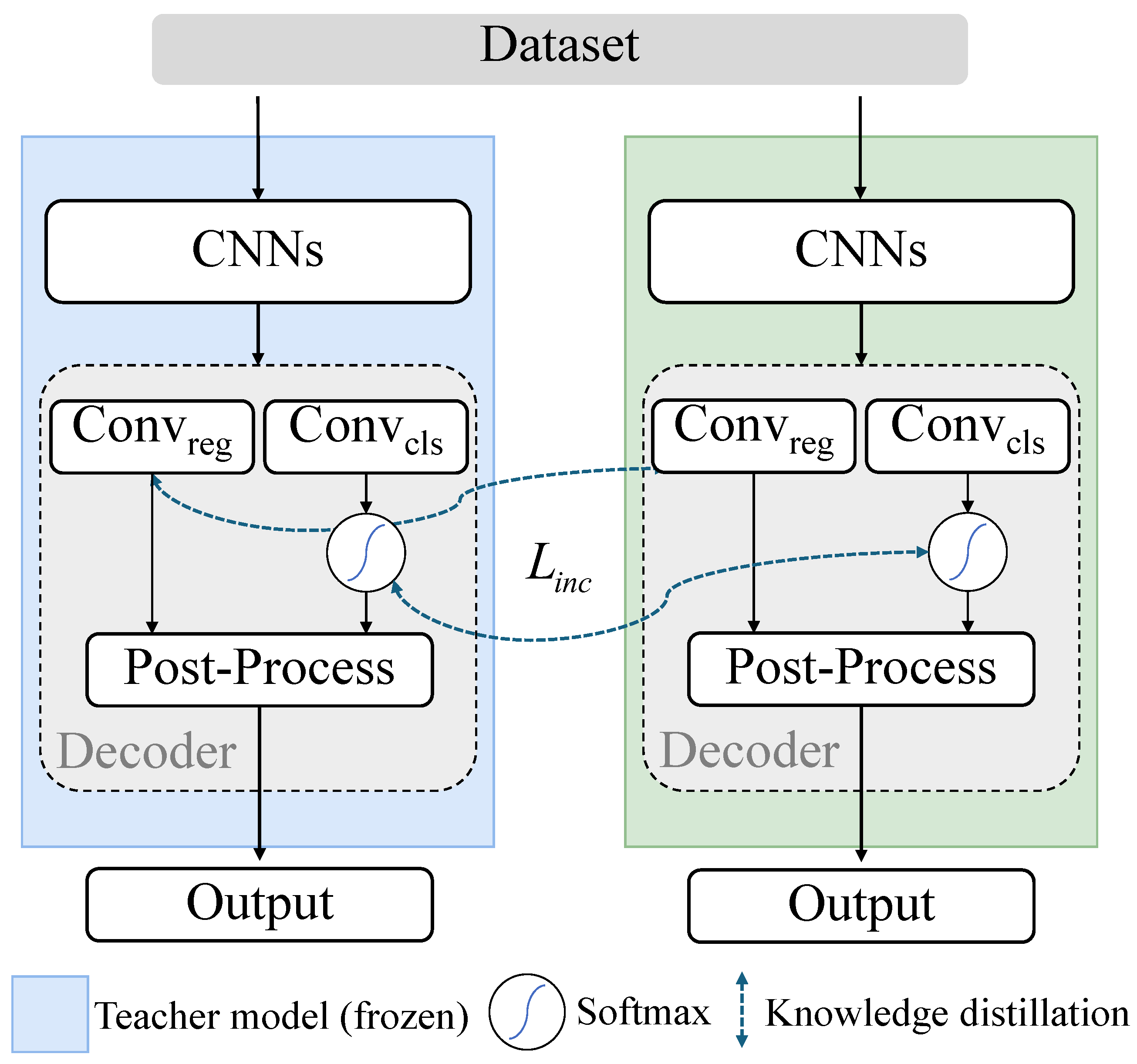
Incremental target detection (ITD) is a method that allows for iterative updates using new data to adapt to novel target detection requirements based on a pre-existing model, with a central aim of preventing the complete erasure of old knowledge. The target detection approach leveraging knowledge distillation extends the original model by adding new branches to achieve model adaptation. The original model, which remains frozen, acts as a guide to create a feature knowledge transfer pathway between the old and new models. This mechanism further ensures the incremental model’s retention of prior knowledge through knowledge distillation. Given that the core functions of the detector—localization and recognition—are performed by the regressor and classifier, respectively, the incremental detector also requires modifications to both the regressor and classifier. The overall framework is shown in Figure 2.
The classifier needs to be expanded before incremental training. Suppose the number of classes in the original dataset is m and the new data is n classes. Then the classification branch will be expanded from m + 1 layers to m + n + 1 layers. When the training is performed, the first m + 1 layers are fine-tuned by the output of the m + 1 layers of the old model, and the last n layers are trained with new knowledge from the new data.
Modification of the regressor is further complicated by the fact that the regressor output is not probability distributed and does not satisfy the requirements of knowledge distillation. Some incremental target detection methods treat localization as a “class-independent” function and simply freeze or fine-tune the regressor parameters, but more recent work has shown that this approach is ineffective in the presence of persistent data increments. For this reason, we refer to the work in [25], which uses GFL as the underlying target detector. GFL proposes a general representation of the regression boundaries, which allows the regression output to be transformed into a probability distribution. For B = l , r , t , b , each of its coordinate positions y is transformed as follows:
y = [ y 0 , y 1 , y k ] Δ i = y i y i 1 , Δ i = Δ j , i , j { 1 , 2 , 3 k }
y i * = i = 0 k S ( p r e d ( i ) ) · i i = 0 k S ( p r e d ( i ) ) · Δ = 1
where Δ is the discretization step of the offset (bin width) and K is the number of bins. S · denotes the SoftMax operator applied to the regression logits to obtain the class distribution over the bins, and y * denotes the SoftMax weighted expectation reconstructed from the discrete distribution. The transformed boundary position is notated as { p l , p r , p t , p b } and subsequently engaged in the incremental learning process through knowledge distillation.
Based on this, this study incorporates wavelet variation concepts and proposes a method optimized for SAR incremental target detection. Section 3.2 explores the correlation between frequency-domain and layer-degree features, setting the stage for subsequent methods. Section 3.3 presents the Hierarchical Frequency-Knowledge Reconstruction (HFKR) method, which enables multi-frequency reconstruction of detector features. HFKR corrects the incremental training process via knowledge distillation, mitigating the feature characterization mismatch problem in non-smooth SAR data increments.

3.2. Frequency Domain-Granularity Feature Correlation

Convolutional neural networks (CNNs) typically comprise multiple layers of convolutional kernels. Shallow layers are designed to capture intuitive features with smaller receptive fields, targeting basic image patterns like edges and textures. These patterns are highly generalizable across diverse tasks and datasets. Conversely, deep layers construct more advanced semantic information by integrating shallow features. This information is more abstract and task-specific, focusing on details such as structural relationships between parts.
An ideal incremental training process should acquire new high-level semantic features while keeping generic features intact. Previous studies, such as [23,24,25], attempt to preserve old knowledge via knowledge distillation with partial parameter freezing; however, this strategy often neglects the correlation between hierarchical features (generic bases vs. detailed cues). High-level semantics are built upon and refine generic features, while parameter freezing makes it difficult to establish or update such cross-level dependencies, leaving the model to rely largely on the pre-increment generalizability of the base network. Moreover, both generalizability and plasticity have been shown to diminish as increments accumulate [50,51], further undermining continual learning. To mitigate this, one line of work introduces explicit feature learning during incremental training to relate generic and detailed features across teacher and student [24,52]; a straightforward attempt is to fuse shallow teacher features with deeper student features (and vice versa) or to integrate them via feature-level distillation. Yet such naïve fusion/distillation is prone to knowledge confusion because the hierarchy of features does not precisely match the hierarchy of semantics: deep features mainly encode coarse, generic information, whereas shallow features often contain fine local details [53,54]. In addition, heterogeneous feature-scale distributions make the tuning of fusion strengths sensitive, which is particularly problematic for SAR imagery with sparse feature evidence [55,56]. These limitations motivate an approach that decouples generic components from detailed components and then aligates them instead of indiscriminately fusing them.
To tackle this challenge, this study introduces wavelet transformation to build a feature decoupling framework. Wavelet transform, a tool for time-frequency localization analysis, decomposes signals across multiple scales using scalable and translatable wavelet basis functions. This approach captures local signal features in both time and frequency domains. Unlike Fourier global analysis, wavelet basis functions can adaptively analyze both high-frequency transient components and low-frequency slow components by adjusting scale and translation factors. Practically, the discrete wavelet transform (DWT) creates a multi-resolution analysis framework by discretizing the scale ( a = 2 j ) and translation ( b = k 2 j ) parameters in a binary manner:
L L = h h f L H = g h f H L = h g f H H = g g f
With h and g representing the low-pass and high-pass filters, respectively, and ↓ denoting the downsampling operation, this process decomposes the image into a low-frequency approximation component ( L L ) and three high-frequency detail components ( L H , H L , H H ). The multiscale characteristic of this technique offers a significant advantage in image processing. The low-frequency sub-bands preserve the main structure of the image, while the high-frequency sub-bands capture detailed features such as edge textures.
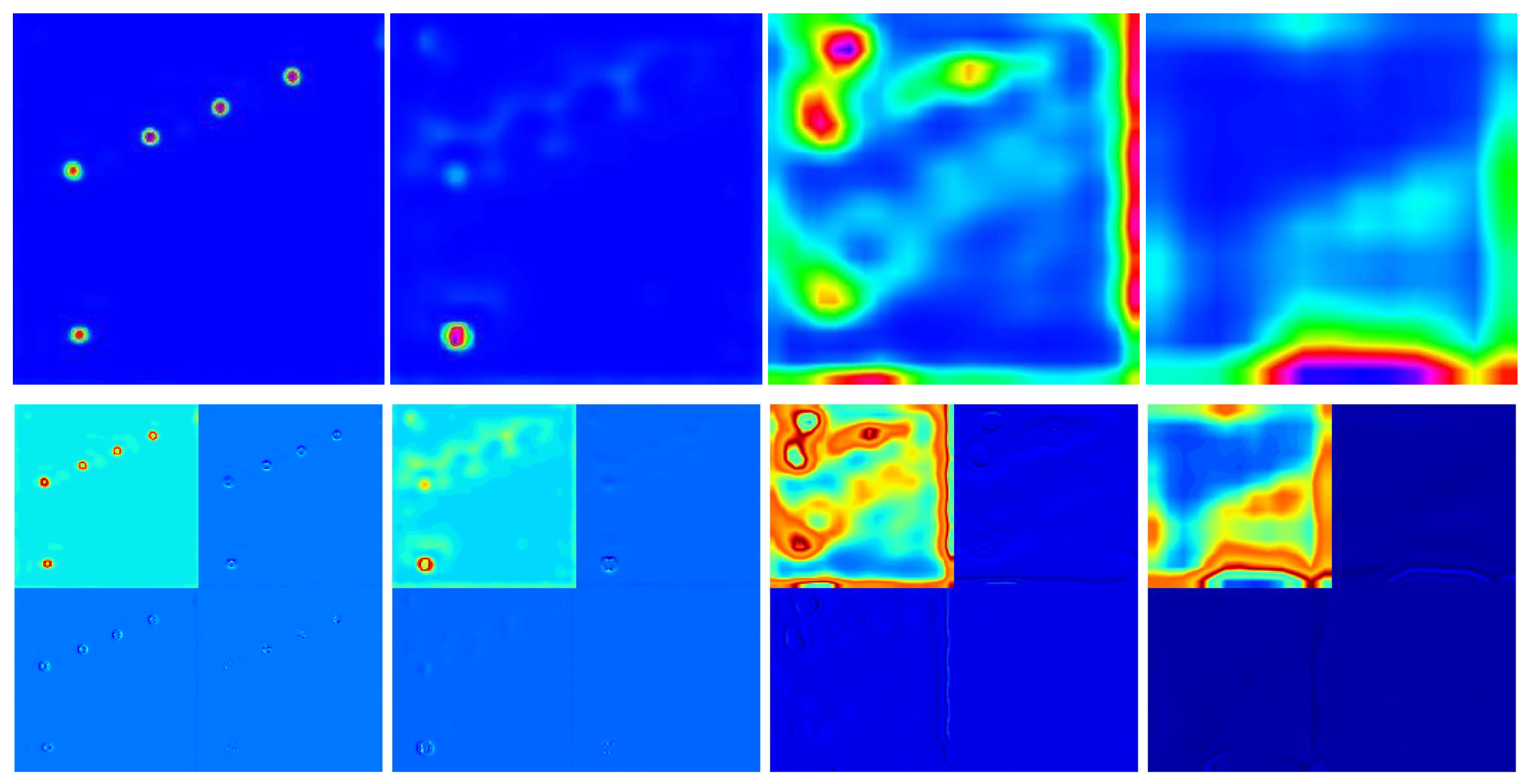
The multi-scale property of wavelet transform provides ideas for solving the feature representation mismatch problem. The feature maps and frequency maps are illustrated in Figure 3. It can be observed that shallow feature attention primarily focuses on the target itself, while deeper layers increasingly attend to the surrounding contextual regions. After wavelet decomposition, the low-frequency components provide clearer contour information, particularly in shallow layers. It is evident that low-frequency components (LL) preserve the core structural information of targets, particularly in shallow layers, while high-frequency components capture more localized, detailed variations. To demonstrate the potential of the wavelet transform for feature decoupling, we conduct a correlation analysis between frequency features and hierarchical features, referred to as frequency–hierarchical correlation verification. Our motivation is to test whether a frequency-domain view can separate depth-dependent semantics and whether this relation persists when the model is trained with different class coverage.
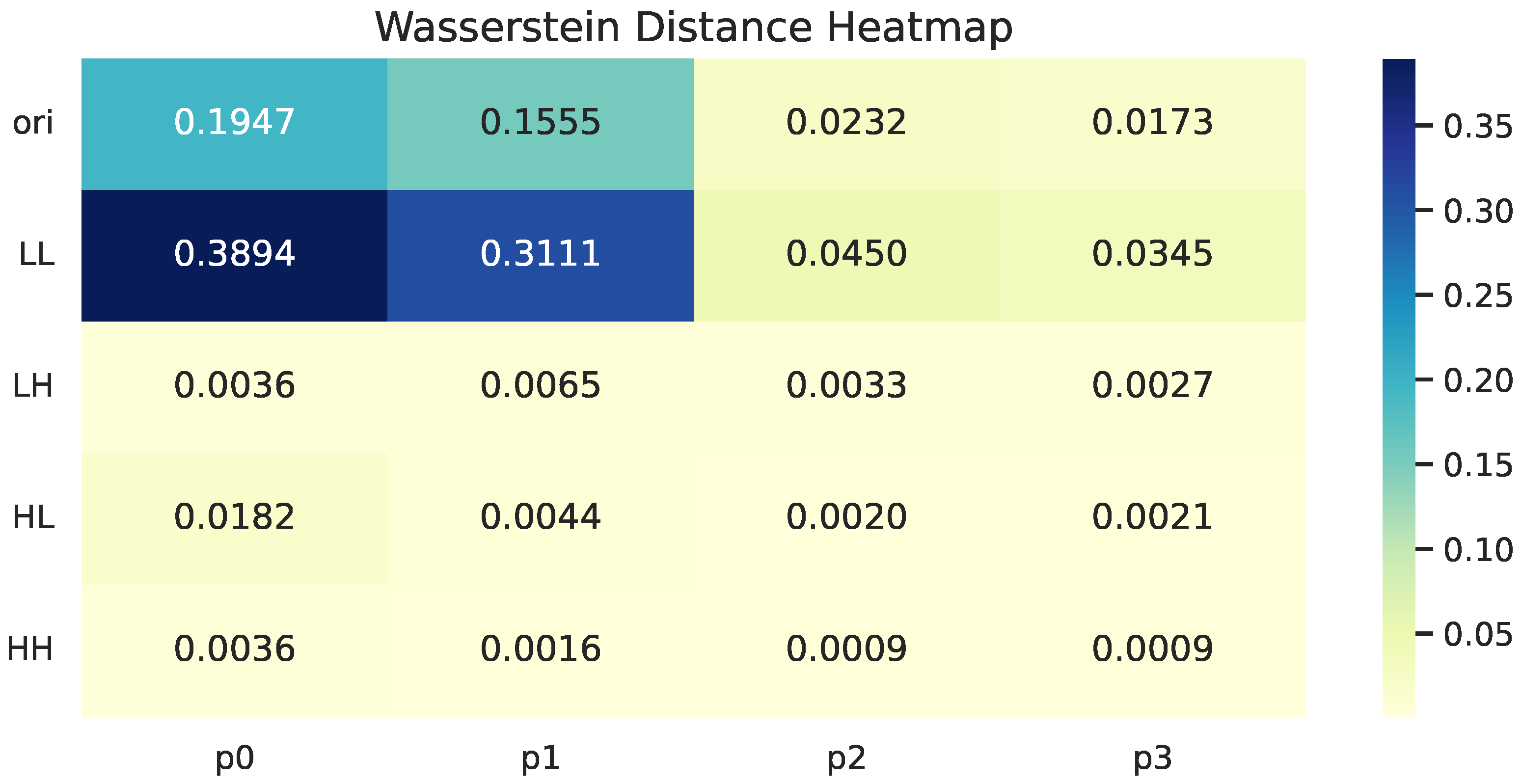
RetinaNet is employed as the base detector. We construct two data settings: D 1 contains only ship and bridge, while D 2 is the full MSAR dataset (held-out splits are used for validation). We first train an offline model M 1 on D 1 , and then perform training to obtain M 2 on D 2 under the same architecture and protocol. For a fair comparison, the analysis is restricted to the shared classes (ship, bridge). At each pyramid level p 0 p 3 , we extract the spatial feature map (ori) of M 1 / M 2 and its separable-DWT sub-bands { LL , LH , HL , HH } . Similarity is quantified by the 1-Wasserstein distance between corresponding activation distributions: for each channel, spatial positions are flattened to form an empirical 1-D distribution; distances are computed channel-wise and summarized as heatmaps. We report (i) inter-layer relations within each model (pairs of ( 1 , 2 ) across p 0 p 3 ), and (ii) cross-model alignment between M 1 and M 2 on the shared classes, with emphasis on the depth-wise evolution of similarity from p 0 to p 3 and on how the spatial maps (ori) compare with the frequency sub-bands { LL , LH , HL , HH } in terms of similarity and difference. This setup makes explicit what is compared and why, and it bridges the mismatch analysis above with the forthcoming W 1 -based quantification.
The Wasserstein Distance (also known as the Earth Mover’s Distance, EMD) [57,58] is a metric used to quantify the spatial distribution differences between two feature maps. It calculates the minimum cost required to transform one feature map into another by optimizing a transport cost function, offering superior sensitivity to spatial structural variations and distributional shifts compared to L2 distance or cosine similarity. Given two 2D feature maps F 1 , F 2 R H × W , we first flatten and normalize them into discrete distributions:
a = vec ( F 1 ) F 1 , b = vec ( F 2 ) F 2
To retain spatial structure, we define a cost matrix C R n × n , where n = H × W , and each entry corresponds to the Euclidean distance between two pixel positions:
C i j = x i x j 2 x i , x j { ( h , w ) h = 1 , , H ; w = 1 , , W }
The discrete Wasserstein-1 distance is then given by the following optimal transport formulation:
W 1 ( a , b ) = min T Π ( a , b ) i = 1 n j = 1 n T i j · C i j
where T R + n × n is the transport plan and Π ( a , b ) denotes the set of admissible couplings:
Π ( a , b ) = T R + n × n | T 1 = a , T 1 = b
After validation, the results are obtained as shown in Figure 4. As the network depth increases, feature maps exhibit reduced inter-layer correlation, thereby validating our earlier hypothesis regarding hierarchical features. Simultaneously, the frequency-domain representations obtained through wavelet decomposition reveal a more distinct hierarchical structure. The low-frequency components at each level exhibit higher correlations compared to the original feature maps, with this effect being especially pronounced in shallow layers. The high-frequency feature components display greater variability, supporting the observed feature mismatches in Figure 1 and the associated model misclassifications. Therefore, based on the preceding analysis and experimental validation, the following two conclusions can be drawn:
  • The multi-scale nature of wavelet transform enables the decomposition of original mixed features into a well-defined hierarchical structure in the frequency domain.
  • Low-frequency features capture the spatial relationship between edges and their positions, exhibiting a degree of generalizability; high-frequency features encode fine-grained discriminative details of targets and are more sensitive to variations in target appearance.

3.3. Hierarchical Frequency-Knowledge Reconstruction (HFKR)

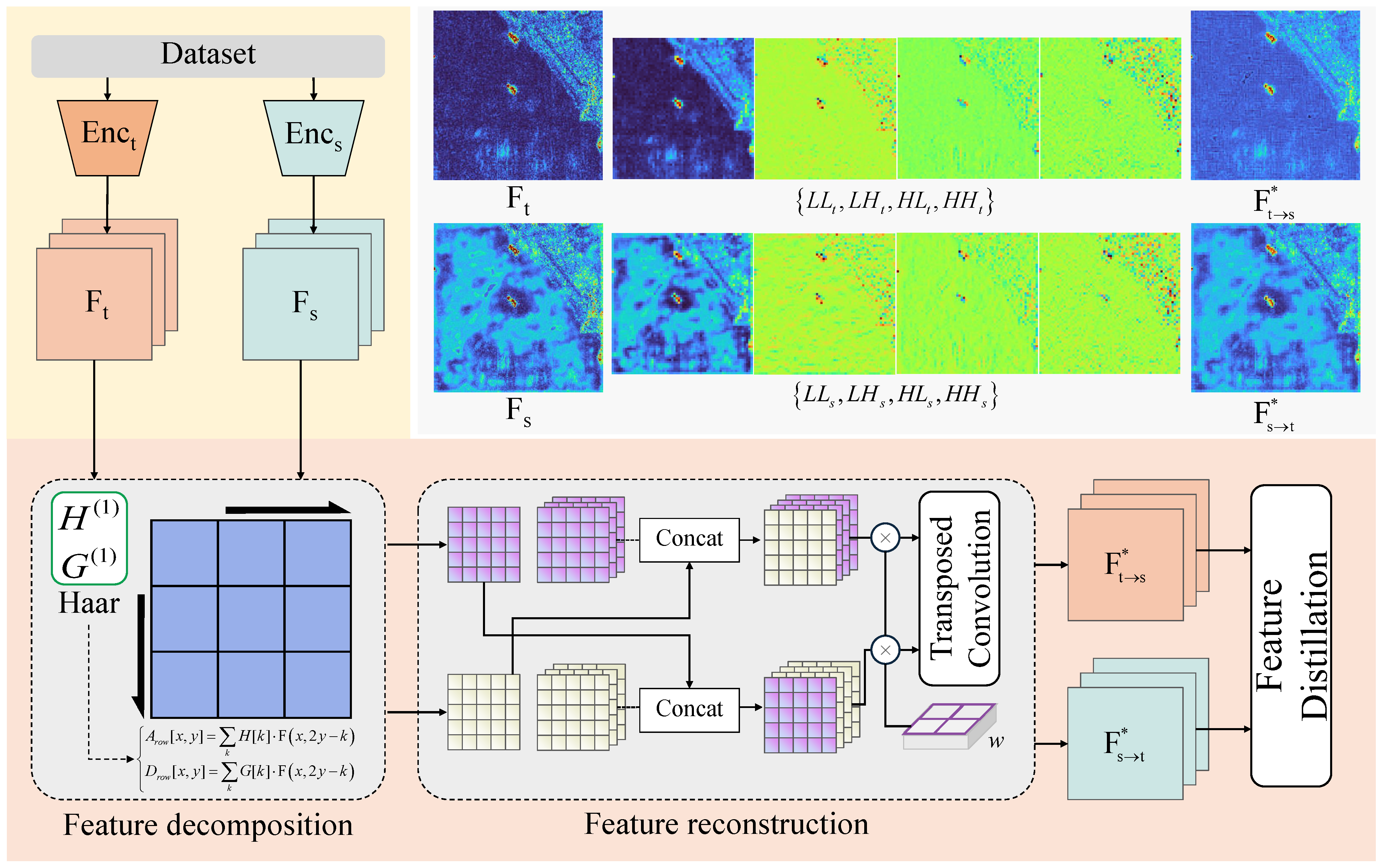
Based on the idea in Section 2, we design the frequency-space decoupled distillation for SAR incremental target detection, called HFKR. As shown in Figure 5, HFKR mainly includes three stages: feature decomposition, feature reconstruction, and fused feature distillation.
HFKR acts in the feature transfer stage and its input is the feature map of the teacher model and the student model. Given the feature map F R C × W × H , each row of the feature map is low-pass and high-pass filtered and downsampled:
F r L [ x , y , c ] = u G [ u ] F [ x , y + u , c ] F r H [ x , y , c ] = u H [ u ] F [ x , y + u , c ]
In Equation (8), F denotes the feature map tensor and square brackets [ · ] indicate indexing, whereas parentheses ( · ) denote function/application. Equation (8) implements the first stage of the separable 2D DWT as a one-dimensional (1-D) analysis filter along the y dimension (within each row). For a given channel c and fixed row index x, the sequence { F [ x , y , c ] } y is convolved with the low-pass filter G and the high-pass filter H, yielding the intermediate responses F r L and F r H . Here, the superscripts L / H denote low/high-pass outputs and the subscript r marks the row-wise stage; the summation index u enumerates filter taps and y + u is the shifted position along the filtered dimension. In this paper, the default Haar in the method exploration phase (we will compare it in more detail in the ablation experiment section) has wavelet coefficients of
H = [ 1 2 , 1 2 ] , G = [ 1 2 , 1 2 ]
Performing the same operation on each column of the result of the previous step results in four sub-feature maps, each of which is 1 4 the size of the original feature map. The calculation procedure is as follows:
F L L [ x , y , c ] = v G [ v ] F r L [ x + v , y , c ] , F L H [ x , y , c ] = v G [ v ] F r H [ x + v , y , c ] , F H L [ x , y , c ] = v H [ v ] F r L [ x + v , y , c ] , F H H [ x , y , c ] = v H [ v ] F r H [ x + v , y , c ] .
Through feature decomposition, the feature maps from both the original model (teacher model) and the student model are decomposed into one set of low-frequency maps (LL) and three sets of high-frequency maps (LH, HL, HH). After each incremental training, prior knowledge is rapidly replaced by new knowledge due to the extreme imbalance of the information before and after. This loss includes not only the detailed features in the new data but also the generic features closely related to the low-frequency maps, as well as the relationship between the generic and detailed features in each task. To mitigate this phenomenon, the idea of this paper is to separate the generic features from the detailed features and establish the correlation between the old and new features of a multi-task by cross-combining and reconstruction. Let the feature maps of the teacher model and the student model be denoted as F t and F s , the decomposition of the above process yields d w t t = { L L t , L H t , H L t , H H t } , d w t s = { L L s , L H s , H L s , H H s } . Combining the low-frequency map of the teacher model with the high-frequency map of the student model, while combining the high-frequency map of the teacher model with the low-frequency map of the student model, we get the following:
d w t t s = { L L t , L H s , H L s , H H s } d w t s t = { L L s , L H t , H L t , H H t }
The recombined frequency domain maps are reconstructed, using an inverse variation method to fuse d w t t and d w t s into new feature maps F t s and F s t . The calculation is as follows:
F * = I W T ( d w t , w ) = 1 2 i { L L , L H , H L , H H } d w t i w i
where w denotes the filter kernel and ⊗ is the transposed convolution (inverse convolution) operation. For the haar wavelet used in this paper, w takes the value:
w L L = 1 1 1 1 , w L H = 1 1 1 1 w H L = 1 1 1 1 , w L H = 1 1 1 1
F t s * includes the low-frequency features from the teacher model and the high-frequency features from the student model, whereas F s t * includes the high-frequency features from the teacher model and the low-frequency features from the student model. To integrate the fused feature maps into the incremental learning process, we combine feature distillation to create a new loss function, L o s s h f k r . The calculation of L hfkr is detailed in Equation (14). In this context, C × W × H denotes the feature map size (number of channels C, width W, and height H), and f i , j , k represents the feature value at the i-th channel, j-th column, and k-th row.
L o s s h f k r = 1 C W H F t s * F s t * 2 = 1 C W H i = 1 C j = 1 W k = 1 H f i , j , k t s f i , j , k s t 2
Let LL t , HF t and LL s , HF s denote the low-/high-frequency components (HF aggregates { LH , HL , HH } ) of the teacher (t) and student (s). We form cross-composed reconstructions F t s * = IDWT ( LL t , HF s ) and F s t * = IDWT ( LL s , HF t ) . If structural (LL) cues are aligned and detail (HF) cues are compatible across models, the two reconstructions should be close; thus Equation (14) enforces a symmetric consistency. With an orthonormal wavelet basis (Parseval):
F t s * F s t * 2 2 = LL t LL s 2 2 + HF s HF t 2 2
So, minimizing Equation (14) is equivalent to jointly aligning low-frequency structure and high-frequency details. This matches Section 3.2, where LL is depth-wise stable and HF captures the divergent fine semantics.
At this stage, the total loss function for incremental training is formulated as shown in Equation (16). The standard learning loss, denoted as L o s s g e n , corresponds to the objective of acquiring knowledge from newly introduced classes and follows the same optimization process as in conventional offline training. The incremental loss, L o s s i n c , reflects the knowledge retained from the original model through knowledge distillation and consists of two components: the incremental classification loss L o s s c l s and the incremental localization loss L o s s r e g .
L o s s = L o s s g e n + α L o s s c l s i n c + L o s s r e g i n c + λ L o s s h f k r
The parameters α and λ in the loss function serve as balancing coefficients. Specifically, α controls the contribution of the incremental localization loss, while λ modulates the influence of the proposed HFKR loss, L o s s h f k r , thereby achieving a trade-off among competing training objectives. In practice, α typically follows the configuration adopted in prior works, whereas the selection of λ is analyzed in detail in the experimental section of this paper.

4. Results

4.1. Datasets

We evaluate the proposed method on the MSAR and SARAIRcraft-1.0 datasets. MSAR is a four-class SAR target dataset comprising 28,449 images and 60,456 targets, sourced from the Hisea-1 and Gaofen-3 satellites. SARAIRcraft-1.0 includes 4368 images and 16,463 aircraft targets across seven classes, using Gaofen-3 satellite data. Detailed dataset statistics are provided in Table 1.
Before incremental training, the dataset must be preprocessed. Since some images include target classes unrelated to the current task, we label only the relevant classes. For example, if bridge detection is conducted on top of a ship detection model, then during the initial training phase, only ships are labeled in images containing both ships and bridges.
Furthermore, the MSAR dataset suffers from severe class imbalance, which significantly affects detector performance. However, addressing class imbalance is not the focus of this study. To minimize confounding factors, we balanced the MSAR dataset by randomly selecting 3000 ship images and 950 oilcan images for training. After preprocessing, the number of images and targets in the two datasets is summarized in Table 2.

4.2. Experimental Settings

4.2.1. Dataset Split

When new class data becomes available, we first employ an incremental learning approach to quickly update the detection model, enabling it to detect both existing and new classes. We then refine the model through further training. This process is repeated with each new data arrival, resulting in a continuously updated model that can be regarded as a sequence of multiple single-step increments. To simulate this process, the dataset was partitioned as follows in this experiment:
  • MSAR dataset partitioning: Ship and bridge are designated as base classes, while oilcan and airplane are treated as incremental classes.
  • SARAIRcraft-1.0 dataset partitioning: A220 and A320/321 are designated as base classes. A330 and ARJ21 are introduced in the first increment, Boeing737 and Boeing787 in the second, and the class “other” in the third increment.

4.2.2. Validation Metrics

In this study, mean Average Precision ( m A P ) is used to evaluate the performance of the detector. A predicted box is considered correctly localized when its Intersection over Union (IoU) is greater than or equal to 0.5, and the corresponding accuracy metric is referred to as m A P 50 .
The calculation of m A P is illustrated in Equation (17), where p and r denote precision and recall, respectively. n recall values are sampled in ascending order, and p i + 1 indicates the precision at recall level r i + 1 . K denotes the number of categories, and the mean of A P values across all classes is taken as the m A P .
A P = i = 1 n 1 ( r i + 1 r i ) · p i + 1 { r 1 , r 2 r n } m A P = 1 K j = 1 K A P j

4.3. Instantiation Under GFL

In our experiments, the base detector is GFL. We use the standard GFL head loss for general training:
Loss gen = QFL + λ DFL DFL + λ IoU IoU
For incremental learning, we adopt logit distillation on old classes:
Loss inc _ cls = τ 2 KL softmax ( z t / τ ) softmax ( z s / τ )
and distributional distillation on the GFL discrete regression distributions:
Loss inc _ reg = sides KL P t bbox P s bbox

4.4. Ablation Study

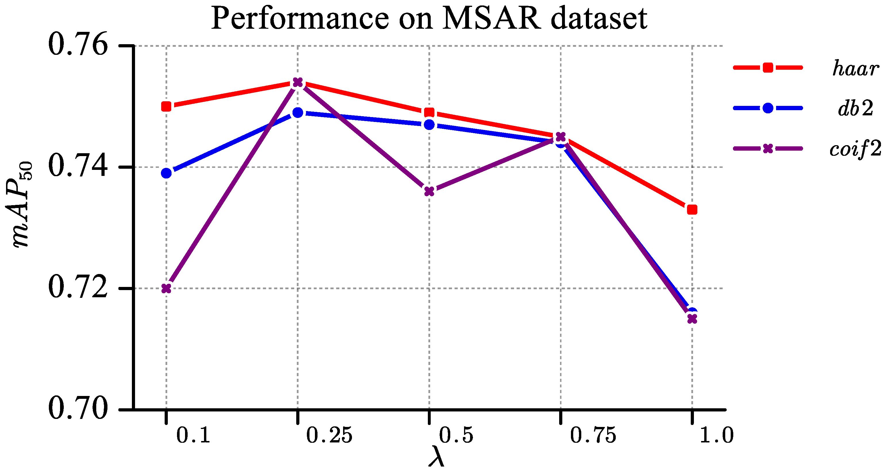
To explore the intrinsic mechanisms of HFKR and its sensitivity to design parameters, we conducted joint ablation experiments focusing on two key components: the coefficient λ and the selection of the wavelet basis for frequency decomposition. According to the work [24,52], the coefficient λ typically ranges from 0.1 to 1. We selected five representative values—0.1, 0.25, 0.5, 0.75, 1—to examine the influence of λ on detection performance. Furthermore, we hypothesize that the choice of wavelet basis affects HFKR performance and is inherently linked to the value of λ . Accordingly, we selected three commonly used wavelets—Haar, db2, and Coif2—whose corresponding bases are illustrated in Table 3.
We tested the detection results under each combination of wavelet and λ , as shown in Figure 6. It can be observed that all three wavelet bases achieve optimal performance when the value of λ is 0.25 or 0.5. Although coif2 achieves comparable performance to haar, it is less stable and computationally efficient. Therefore, haar is selected as the wavelet basis and the value of λ is set to 0.25 in this study.
Furthermore, we utilize the MSAR dataset to validate the effectiveness of HFKR. We follow the data splitting protocol described in the previous section. As shown in Table 4, the model demonstrates improved detection performance after incorporating HFKR. Except for the bridge class, where the detection performance is slightly lower than that of the original method, the proposed model outperforms in all other classes. In particular, the detection performance for the oilcan and airplane classes is significantly improved, with an overall performance gain of 4.5% compared to the original method. These results demonstrate the enhanced effectiveness of the HFKR-based SAR incremental target detection method.

4.5. Comparison with Other Methods

Next, we evaluate the performance of the proposed method through comparative experiments. The proposed method is built upon the GFL [45] detection framework. Comparison methods include RILOD [40], SID [24], ERD [25], IDCOD [42], and Tian [41], which are representative approaches from recent years. To ensure fair comparisons unaffected by the base detector, all methods are re-implemented within the GFL-based framework. All methods are trained under the same basic settings and number of epochs to ensure fairness. Hyperparameters for the comparison methods follow the descriptions in their respective papers and are tuned within a small range to achieve optimal performance.
Section labeling instructions:
  • Red: The best effect of current item
  • Blue: The second-best effect of current item
  • *: Reproduced from the original article (the work was not provided with source code)
  • †: Porting its provided source code into the unified framework (GFL).

4.5.1. Experiments on the MSAR Dataset

Table 5 presents the performance comparison of different incremental detection methods on the MSAR dataset under the (2 + 2) setting, where two base classes (ship, bridge) are followed by two incremental classes (oilcan, airplane). The proposed method, denoted as Ours (with HFKR), achieves the highest overall mAP (75.4%) among all competing approaches, exceeding the next-best method by a margin of 2.0% and narrowing the performance gap to the full-data upper bound (FD) to only 4.1%.
In terms of class-wise performance, our method obtains the best detection results in oilcan and airplane, which are both incremental classes, with mAP values of 97.3% and 58.9%, respectively. This indicates the effectiveness of the proposed Hierarchical Frequency-Knowledge Reconstruction (HFKR) module in preserving model plasticity and ensuring feature alignment across tasks. Although there is a minor drop in the bridge class (71.6% vs. 73.4% in SID), our approach maintains competitive performance on base classes overall, with an old-class mAP of 72.7%.
Compared with representative baselines such as ERD (72.6%) and IDCOD (73.1%), our method demonstrates superior stability in retaining old knowledge while integrating new classes. Moreover, SID shows a drastic drop in new-class performance (45.1%), highlighting the limitations of relying solely on parameter isolation. In contrast, HFKR effectively mitigates feature representation mismatch, leading to balanced improvements across both old and new tasks.
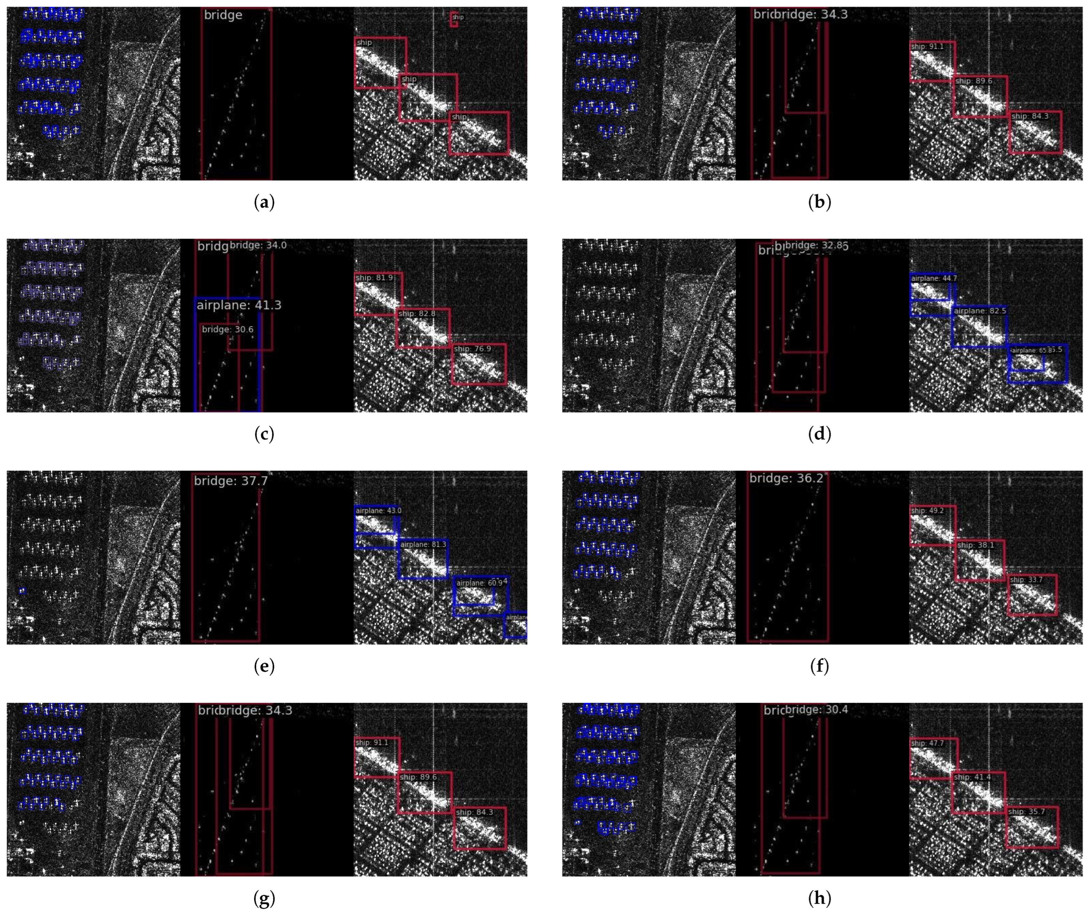
Figure 7 presents a qualitative comparison of detection results from multiple incremental learning methods on the MSAR dataset. The ground truth annotations (leftmost) serve as a reference for evaluating the detection quality of each approach. Traditional methods such as RILOD and SID exhibit evident localization errors and miss several targets, particularly in dense or cluttered regions. ERD and IDCOD demonstrate improved target coverage, but still suffer from false positives or incomplete bounding in complex scenarios. In contrast, the proposed method (Ours) achieves detection results that are closest to the ground truth, exhibiting both accurate localization and superior completeness. Compared with the best-performing baselines (e.g., Tian), our method provides more consistent detection across multiple instances while reducing background interference. This improvement can be attributed to the proposed Hierarchical Frequency-Knowledge Reconstruction (HFKR) mechanism, which enhances feature transfer by aligning cross-level frequency information and stabilizing inter-task representation.

4.5.2. Experiments on the SARAIRcraft Dataset

The SARAIRcraft dataset contains a greater variety of classes, therefore, we conducted multi-step incremental experiments on it. The experimental results are presented in Table 6, demonstrating that our method consistently outperforms others at each incremental stage. In the initial stage, our method significantly outperforms all baseline approaches. It achieved the highest detection rates for the A220, A320/321, and A330 classes. Our approach exceeds the second-best method (SID) by 3.2% in m A P and is only 4.3% behind the upper performance bound (FD), making it the only method within 5% of FD across all approaches.
In the second stage, all methods—except RILOD—achieved performance within 10% of FD. ERD achieved the best performance on the old class with a detection rate of 74.5%. Our method, along with SID, achieved the second-best performance on the old class. For the new class, IDCOD and Tian were the top-performing methods, with detection rates of 66.9% and 65.9%, respectively. Although our method did not achieve the highest performance on either the old class or the new class, it still attained the highest overall m A P of 70.5%, outperforming all other methods due to its more stable performance. Moreover, the gap with FD was reduced to 2.7%, which is 2.1% smaller than that of the next best method.
In the third stage, the performance differences between methods became more pronounced. Three methods—RILOD, IDCOD, and Tian—show a gap of more than 8% from FD, whereas the remaining methods are within a 5% gap. Our method achieves the best performance on the A330 class and second-best results across all other classes. ERD performs exceptionally well on the old classes; however, it achieves the poorest results on the new classes, with a 13.4% gap from FD. Our method achieved second-best detection results on both old and new classes, with a m A P of 74.0%, representing the best overall performance across all categories. It is worth noting that although our method achieved the best performance in each stage, its performance margin is gradually narrowing, indicating a potential limitation that warrants further investigation.
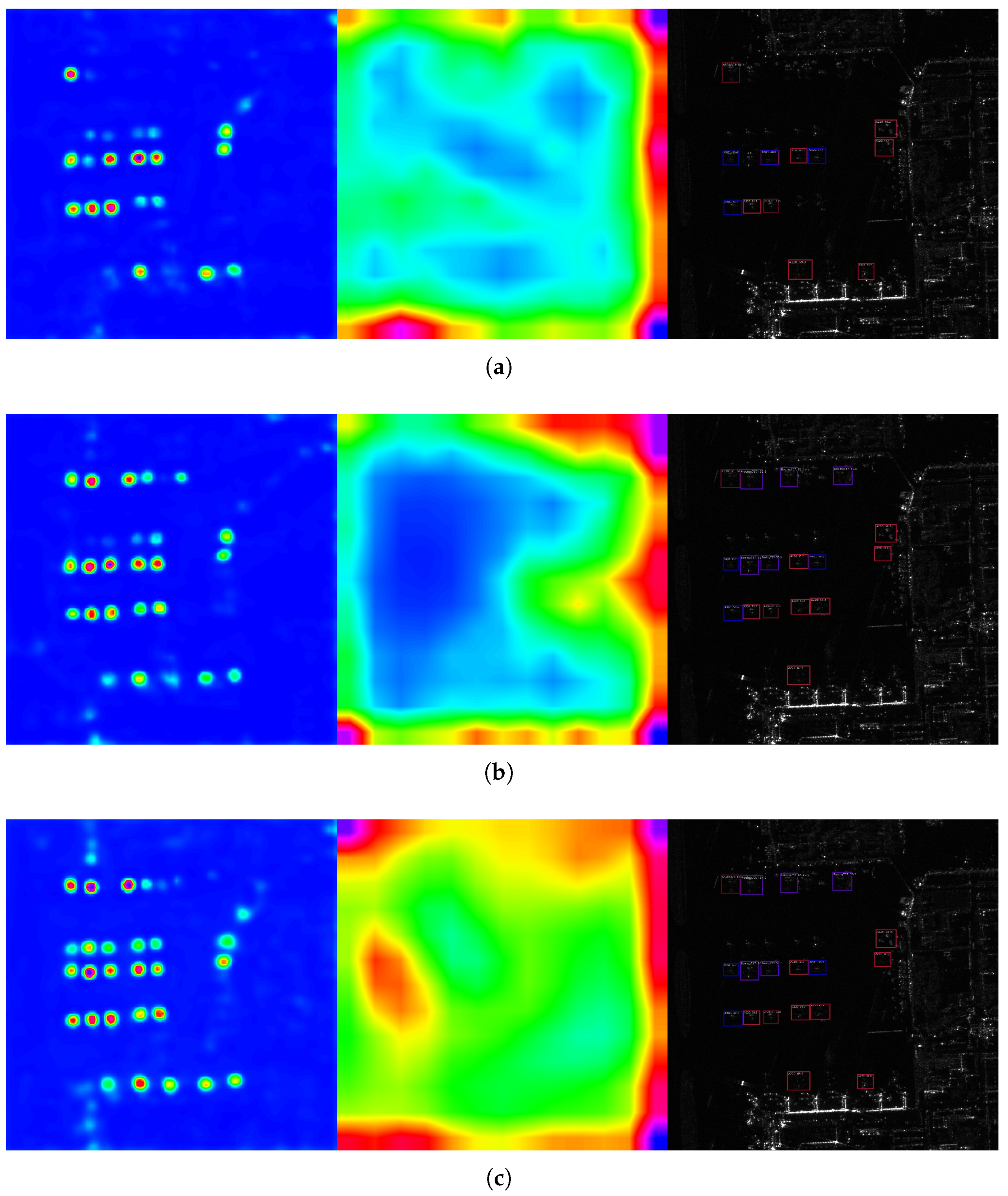
Additionally, to investigate the stability of feature representations across incremental stages, we visualize shallow (p0) and deep (p3) features, along with detection results on the SARAIRcraft dataset. Figure 8 and Figure 9 illustrates the evolution of feature distributions and detection outcomes over three incremental learning stages. As shown in the p0 feature plot, traditional incremental methods often produce noisy and unstable activations, particularly when new classes are introduced. In contrast, our method maintains consistent low-level representations, preserving essential contour and texture information throughout the learning process. The stability of shallow features contributes to effective background discrimination and overall scene understanding. During the incremental learning of deep features, attention drift becomes more pronounced. However, compared with Figure 1, the proposed method exhibits the least feature distortion, which can be attributed to HFKR’s ability to maintain stage-wise feature consistency through frequency-guided feature alignment. Furthermore, experimental results confirm that our method maintains high confidence and accurate localization for both previously learned and newly introduced categories. These findings also underscore the importance of consistent feature representations in long-term incremental learning.

5. Discussion

This section presents a comprehensive analysis of the results discussed in Section 4. The analysis focuses on three key aspects: the overall effectiveness of our method, its performance trends under multi-step incremental settings, and its potential applicability to related domains.

5.1. Overall Effectiveness

The results indicate that the main advantage of the proposed method lies in its overall performance across all classes, rather than superior performance in individual class. As shown in Table 6, our method consistently achieves the highest m A P across all incremental learning phases. However, when examining performance by individual class, it becomes evident that our method does not consistently outperform all baselines. In certain classes, earlier methods and even simpler frameworks achieved slightly better results. This phenomenon suggests that the strength of the proposed method lies in its ability to balance performance between old and new classes, rather than optimizing a specific subset.
This balance is particularly important in real-world SAR target detection scenarios, where overfitting to specific or newly introduced classes can undermine the reliability of long-term models. The ability of the proposed method to maintain high average performance while preserving previously learned knowledge reflects more robust and stable learning dynamics.
Meanwhile, we observe that the airplane class attains a noticeably lower AP than the other categories, whereas the bridge class exhibits pronounced scene-dependent variability: performing poorly in some scenes but very strongly in others. We attribute this to the following factors:
  • Fewer airplane samples in MSAR. Airplane has the smallest class size in our split, which weakens calibration and generalization compared with ship.
  • Small and clustered targets. Airplane targets are typically small and spatially concentrated, this increases localization ambiguity and makes detection intrinsically harder.
  • Bridge size and scene variability. Bridge targets are generally larger than other classes in MSAR and span complex backgrounds (river/urban scenes). Their elongated geometry causes unstable performance in certain scenes despite the larger absolute size.
In future work, we will incorporate small-target augmentations, class-rebalancing, and shape-aware assignment to mitigate the gap while keeping the overall incremental protocol unchanged.

5.2. Performance Trends

Another noteworthy observation is that the advantage of the proposed method gradually diminishes across successive incremental phases. Although the proposed method maintains the best performance at each stage, the performance gap between it and other methods narrows over time. This trend is clearly reflected in the transition from Inc (2 + 2) to Inc (6 + 1), as shown in Table 6. This highlights a critical direction for future improvement.

5.3. Potential Applicability to Related Domains

Finally, based on the above analysis, we believe that the proposed method has strong potential to be effectively applied to other SAR image analysis tasks. The stable performance demonstrated at each stage suggests that the proposed method possesses a certain degree of generalizability across varying data conditions, along with a strong capacity to balance new and old class knowledge. Such challenges are also prevalent in small-sample learning and domain adaptation tasks. This indicates that our method is applicable not only to class-incremental detection tasks but also to hybrid scenarios involving few-shot learning, domain-incremental learning, or even semi-supervised learning paradigms. Such extensions would further validate the versatility and practical value of the proposed method in real-world SAR system applications.

6. Conclusions

Due to the inherent sparsity and sensitivity, SAR images make incremental target detection particularly susceptible to feature representation mismatches between previously learned and newly introduced classes. To address this challenge, this paper first investigates how representation mismatches manifest in SAR-specific scenarios. Through theoretical and experimental studies, it is found that there is a strong correlation between the hierarchical spatial features and their corresponding frequency domain structures. Motivated by this observation, we propose the Hierarchical Frequency-Knowledge Reconstruction (HFKR) method that incorporates wavelet-based frequency decomposition into the incremental learning process. HFKR alleviates the attention shift caused by distribution divergence in the incremental learning process by maintaining hierarchical consistency, and effectively enhances the feature concatenation between old and new tasks. This design is particularly well-suited for SAR applications, where effective feature adaptation plays a crucial role in ensuring robust model evolution.
Trials with multiple data incremental settings verify the effectiveness of our method. HFKR consistently achieves the best performance at each incremental stage, although it does not always lead in per-category accuracy. It is worth noting that as the incremental stage increases, the lead of our method and comparison methods shrinks, which highlights the advantage of HFKR in early adaptation and also points out the future improvement direction. At the same time, we observe that HFKR has good generalization and the ability to balance new and old knowledge, which indicates that the idea of this work has the potential to be extended to related SAR image analysis tasks.

Author Contributions

Methodology, Y.T. and Z.C. (Zongjie Cao); Software, Y.T.; Validation, Y.T. and Z.Z.; Formal analysis, Z.C. (Zongyong Cui); Data curation, Y.T. and Z.Z.; Writing—original draft, Y.T.; Writing—review & editing, Z.C. (Zongyong Cui) and Z.C. (Zongjie Cao); Visualization, Y.T. and Z.Z.; Supervision, Z.C. (Zongjie Cao). All authors have read and agreed to the published version of the manuscript.

Funding

This research was supported by the National Natural Science Foundation of China under Grant 62471112 and 62271116.

Data Availability Statement

The datasets analyzed in this study are publicly available. The MSAR dataset can be accessed at https://radars.ac.cn/web/data/getData?dataType=MSAR, accessed on 19 March 2022. The SAR-AIRcraft-1.0 dataset are available at https://radars.ac.cn/cn/article/doi/10.12000/JR23043, accessed on 17 July 2023.

Acknowledgments

We gratefully acknowledge the Journal of Radars (JRS) Open Data Platform (https://radars.ac.cn) for providing the open SAR datasets that support this work, including MSAR and SARAIRcraft. We also thank the data curators and annotators for their sustained efforts in maintaining high-quality public resources. The views expressed are solely those of the authors.

Conflicts of Interest

The authors declare no conflicts of interest.

Abbreviations

The following abbreviations are used in this manuscript:
HFKRHierarchical Frequency-Guided Knowledge Reconstruction (Proposed)
DWTDiscrete Wavelet Transform
ILIncremental Learning
ITDIncremental Target Detection
KDKnowledge Distillation
EMDEarth Mover’s Distance/Wasserstein Distance

References

  1. Dellinger, F.; Delon, J.; Gousseau, Y.; Michel, J.; Tupin, F. SAR-SIFT: A SIFT-like algorithm for SAR images. IEEE Trans. Geosci. Remote Sens. 2014, 53, 453–466. [Google Scholar] [CrossRef]
  2. Dang, S.; Cao, Z.; Cui, Z.; Pi, Y.; Liu, N. Open Set Incremental Learning for Automatic Target Recognition. IEEE Trans. Geosci. Remote Sens. 2019, 57, 4445–4456. [Google Scholar] [CrossRef]
  3. Qin, X.; Zhou, S.; Zou, H.; Gao, G. A CFAR detection algorithm for generalized gamma distributed background in high-resolution SAR images. IEEE Geosci. Remote Sens. Lett. 2012, 10, 806–810. [Google Scholar]
  4. Du, Y.; Du, L.; Guo, Y.; Shi, Y. Semisupervised SAR Ship Detection Network via Scene Characteristic Learning. IEEE Trans. Geosci. Remote Sens. 2023, 61, 1–17. [Google Scholar] [CrossRef]
  5. Zhou, Z.; Cui, Z.; Tang, K.; Tian, Y.; Pi, Y.; Cao, Z. Gaussian meta-feature balanced aggregation for few-shot synthetic aperture radar target detection. ISPRS J. Photogramm. Remote Sens. 2024, 208, 89–106. [Google Scholar] [CrossRef]
  6. Guo, Y.; Chen, S.; Zhan, R.; Wang, W.; Zhang, J. LMSD-YOLO: A lightweight YOLO algorithm for multi-scale SAR ship detection. Remote Sens. 2022, 14, 4801. [Google Scholar] [CrossRef]
  7. Wang, Z.; Wang, R.; Ai, J.; Zou, H.; Li, J. Global and Local Context-Aware Ship Detector for High-Resolution SAR Images. IEEE Trans. Aerosp. Electron. Syst. 2023, 59, 4159–4167. [Google Scholar] [CrossRef]
  8. Cui, Z.; Wang, X.; Liu, N.; Cao, Z.; Yang, J. Ship detection in large-scale SAR images via spatial shuffle-group enhance attention. IEEE Trans. Geosci. Remote Sens. 2020, 59, 379–391. [Google Scholar] [CrossRef]
  9. Cui, Z.; Li, Q.; Cao, Z.; Liu, N. Dense Attention Pyramid Networks for Multi-Scale Ship Detection in SAR Images. IEEE Trans. Geosci. Remote Sens. 2019, 57, 8983–8997. [Google Scholar] [CrossRef]
  10. Han, S.; Addabbo, P.; Biondi, F.; Clemente, C.; Orlando, D.; Ricci, G. Innovative Solutions Based on the EM-Algorithm for Covariance Structure Detection and Classification in Polarimetric SAR Images. IEEE Trans. Aerosp. Electron. Syst. 2023, 59, 209–227. [Google Scholar] [CrossRef]
  11. Liu, J.; Zhang, T.; Zhang, Z.; Xiong, H. Evaluating the Robustness of Polarimetric Features: A Case Study of PolSAR Ship Detection. IEEE Geosci. Remote Sens. Lett. 2024, 21, 1–5. [Google Scholar] [CrossRef]
  12. Wang, X.; Cao, Z.; Pi, Y. Semisupervised Classification with Adaptive Anchor Graph for PolSAR Images. IEEE Geosci. Remote Sens. Lett. 2022, 19, 1–5. [Google Scholar] [CrossRef]
  13. Tian, Z.; Wang, W.; Zhou, K.; Song, X.; Shen, Y.; Liu, S. Weighted Pseudo-Labels and Bounding Boxes for Semisupervised SAR Target Detection. IEEE J. Sel. Top. Appl. Earth Obs. Remote Sens. 2024, 17, 5193–5203. [Google Scholar] [CrossRef]
  14. Deng, J.; Wang, W.; Zhang, H.; Zhang, T.; Zhang, J. PolSAR Ship Detection Based on Superpixel-Level Contrast Enhancement. IEEE Geosci. Remote Sens. Lett. 2024, 21, 1–5. [Google Scholar] [CrossRef]
  15. Zhao, Y.; Zhao, L.; Ding, D.; Hu, D.; Kuang, G.; Liu, L. Few-Shot Class-Incremental SAR Target Recognition via Cosine Prototype Learning. IEEE Trans. Geosci. Remote Sens. 2023, 61, 1–18. [Google Scholar] [CrossRef]
  16. Xu, W.; Yuan, X.; Hu, Q.; Li, J. SAR-optical feature matching: A large-scale patch dataset and a deep local descriptor. Int. J. Appl. Earth Obs. Geoinf. 2023, 122, 103433. [Google Scholar] [CrossRef]
  17. Li, Z.; Hoiem, D. Learning without forgetting. IEEE Trans. Pattern Anal. Mach. Intell. 2017, 40, 2935–2947. [Google Scholar] [CrossRef]
  18. Dang, S.; Cao, Z.; Cui, Z.; Pi, Y.; Liu, N. Class Boundary Exemplar Selection Based Incremental Learning for Automatic Target Recognition. IEEE Trans. Geosci. Remote Sens. 2020, 58, 5782–5792. [Google Scholar] [CrossRef]
  19. Li, B.; Cui, Z.; Cao, Z.; Yang, J. Incremental Learning Based on Anchored Class Centers for SAR Automatic Target Recognition. IEEE Trans. Geosci. Remote Sens. 2022, 60, 1–13. [Google Scholar] [CrossRef]
  20. Rebuffi, S.A.; Kolesnikov, A.; Sperl, G.; Lampert, C.H. icarl: Incremental classifier and representation learning. In Proceedings of the IEEE Conference on Computer Vision and Pattern Recognition, Honolulu, HI, USA, 21–26 July 2017; pp. 2001–2010. [Google Scholar]
  21. Shmelkov, K.; Schmid, C.; Alahari, K. Incremental learning of object detectors without catastrophic forgetting. In Proceedings of the IEEE International Conference on Computer Vision, Venice, Italy, 22–29 October 2017; pp. 3400–3409. [Google Scholar]
  22. Girshick, R. Fast r-cnn. In Proceedings of the IEEE International Conference on Computer Vision, Santiago, Chile, 7–13 December 2015; pp. 1440–1448. [Google Scholar]
  23. Peng, C.; Zhao, K.; Lovell, B.C. Faster ilod: Incremental learning for object detectors based on faster rcnn. Pattern Recognit. Lett. 2020, 140, 109–115. [Google Scholar] [CrossRef]
  24. Peng, C.; Zhao, K.; Maksoud, S.; Li, M.; Lovell, B.C. SID: Incremental learning for anchor-free object detection via Selective and Inter-related Distillation. Comput. Vis. Image Underst. 2021, 210, 103229. [Google Scholar] [CrossRef]
  25. Feng, T.; Wang, M.; Yuan, H. Overcoming catastrophic forgetting in incremental object detection via elastic response distillation. In Proceedings of the IEEE/CVF Conference on Computer Vision and Pattern Recognition, New Orleans, LA, USA, 18–24 June 2022; pp. 9427–9436. [Google Scholar]
  26. Goodfellow, I.J.; Mirza, M.; Xiao, D.; Courville, A.; Bengio, Y. An Empirical Investigation of Catastrophic Forgetting in Gradient-Based Neural Networks. arXiv 2015, arXiv:1312.6211. [Google Scholar] [CrossRef]
  27. De Lange, M.; Aljundi, R.; Masana, M.; Parisot, S.; Jia, X.; Leonardis, A.; Slabaugh, G.; Tuytelaars, T. A Continual Learning Survey: Defying Forgetting in Classification Tasks. IEEE Trans. Pattern Anal. Mach. Intell. 2022, 44, 3366–3385. [Google Scholar] [CrossRef] [PubMed]
  28. Lin, T.; Maire, M.; Belongie, S.J.; Bourdev, L.D.; Girshick, R.B.; Hays, J.; Perona, P.; Ramanan, D.; Dollár, P.; Zitnick, C.L. Microsoft COCO: Common Objects in Context. arXiv 2014, arXiv:1405.0312. [Google Scholar] [CrossRef]
  29. Everingham, M.; Gool, L.V.; Williams, C.K.I.; Winn, J.; Zisserman, A. The Pascal Visual Object Classes (VOC) Challenge. Int. J. Comput. Vis. 2010, 88, 303–338. [Google Scholar] [CrossRef]
  30. Xu, G.; Zhang, B.; Yu, H.; Chen, J.; Xing, M.; Hong, W. Sparse Synthetic Aperture Radar Imaging From Compressed Sensing and Machine Learning: Theories, applications, and trends. IEEE Geosci. Remote Sens. Mag. 2022, 10, 32–69. [Google Scholar] [CrossRef]
  31. Zhou, H.; Jayender, J. EMDQ: Removal of Image Feature Mismatches in Real-Time. IEEE Trans. Image Process. 2022, 31, 706–720. [Google Scholar] [CrossRef]
  32. Lyu, J.; Bai, C.; Yang, J.W.; Lu, Z.; Li, X. Cross-Domain Policy Adaptation by Capturing Representation Mismatch. In Proceedings of Machine Learning Research, Proceedings of the 41st International Conference on Machine Learning (PMLR), Vienna, Austria, 21–27 July 2024; Salakhutdinov, R., Kolter, Z., Heller, K., Weller, A., Oliver, N., Scarlett, J., Berkenkamp, F., Eds.; Microtome Publishing: Brookline, MA, USA, 2024; Volume 235, pp. 33638–33663. [Google Scholar]
  33. Zhang, T.; Zeng, T.; Zhang, X. Synthetic Aperture Radar (SAR) Meets Deep Learning. Remote Sens. 2023, 15, 303. [Google Scholar] [CrossRef]
  34. Zhang, P.; Xu, H.; Tian, T.; Gao, P.; Li, L.; Zhao, T.; Zhang, N.; Tian, J. SEFEPNet: Scale Expansion and Feature Enhancement Pyramid Network for SAR Aircraft Detection with Small Sample Dataset. IEEE J. Sel. Top. Appl. Earth Obs. Remote Sens. 2022, 15, 3365–3375. [Google Scholar] [CrossRef]
  35. Luo, Z.; Liu, Y.; Schiele, B.; Sun, Q. Class-Incremental Exemplar Compression for Class-Incremental Learning. In Proceedings of the 2023 IEEE/CVF Conference on Computer Vision and Pattern Recognition (CVPR), Vancouver, BC, Canada, 18–22 June 2023; pp. 11371–11380. [Google Scholar] [CrossRef]
  36. Zhang, B.; Luo, C.; Yu, D.; Li, X.; Lin, H.; Ye, Y.; Zhang, B. Metadiff: Meta-learning with conditional diffusion for few-shot learning. In Proceedings of the AAAI Conference on Artificial Intelligence, Vancouver, BC, Canada, 20–27 February 2024; Volume 38, pp. 16687–16695. [Google Scholar]
  37. Yang, Y.; Yuan, H.; Li, X.; Lin, Z.; Torr, P.; Tao, D. Neural Collapse Inspired Feature-Classifier Alignment for Few-Shot Class-Incremental Learning. In Proceedings of the Eleventh International Conference on Learning Representations, Kigali, Rwanda, 1–5 May 2023. [Google Scholar]
  38. Yu, X.; Dong, F.; Ren, H.; Zhang, C.; Zou, L.; Zhou, Y. Multilevel Adaptive Knowledge Distillation Network for Incremental SAR Target Recognition. IEEE Geosci. Remote Sens. Lett. 2023, 20, 4004405. [Google Scholar] [CrossRef]
  39. He, J. Gradient Reweighting: Towards Imbalanced Class-Incremental Learning. In Proceedings of the IEEE/CVF Conference on Computer Vision and Pattern Recognition (CVPR), Seattle, WA, USA, 16–22 June 2024; pp. 16668–16677. [Google Scholar]
  40. Li, D.; Tasci, S.; Ghosh, S.; Zhu, J.; Zhang, J.; Heck, L. RILOD: Near real-time incremental learning for object detection at the edge. In Proceedings of the 4th ACM/IEEE Symposium on Edge Computing, New York, NY, USA, 7–9 November 2019; SEC ’19; pp. 113–126. [Google Scholar] [CrossRef]
  41. Tian, Y.; Cui, Z.; Ma, J.; Zhou, Z.; Cao, Z. Continual Learning for SAR Target Incremental Detection via Predicted Location Probability Representation and Proposal Selection. IEEE Trans. Geosci. Remote Sens. 2024, 62, 5211215. [Google Scholar] [CrossRef]
  42. Feng, H.; Zhang, L.; Yang, X.; Liu, Z. Enhancing class-incremental object detection in remote sensing through instance-aware distillation. Neurocomputing 2024, 583, 127552. [Google Scholar] [CrossRef]
  43. Ren, S.; He, K.; Girshick, R.; Sun, J. Faster R-CNN: Towards Real-Time Object Detection with Region Proposal Networks. In Proceedings of the Advances in Neural Information Processing Systems, Montreal, QC, Canada, 7–12 December 2015; Cortes, C., Lawrence, N., Lee, D., Sugiyama, M., Garnett, R., Eds.; Curran Associates, Inc.: Nice, France, 2015; Volume 28. [Google Scholar]
  44. Zhou, X.; Wang, D.; Krähenbühl, P. Objects as points. arXiv 2019, arXiv:1904.07850. [Google Scholar] [PubMed]
  45. Li, X.; Wang, W.; Wu, L.; Chen, S.; Hu, X.; Li, J.; Tang, J.; Yang, J. Generalized focal loss: Learning qualified and distributed bounding boxes for dense object detection. Adv. Neural Inf. Process. Syst. 2020, 33, 21002–21012. [Google Scholar]
  46. Kirkpatrick, J.; Pascanu, R.; Rabinowitz, N.; Veness, J.; Desjardins, G.; Rusu, A.A.; Milan, K.; Quan, J.; Ramalho, T.; Grabska-Barwinska, A.; et al. Overcoming catastrophic forgetting in neural networks. Proc. Natl. Acad. Sci. USA 2017, 114, 3521–3526. [Google Scholar] [CrossRef]
  47. Perez-Rua, J.M.; Zhu, X.; Hospedales, T.M.; Xiang, T. Incremental few-shot object detection. In Proceedings of the IEEE/CVF Conference on Computer Vision and Pattern Recognition, Seattle, WA, USA, 14–19 June 2020; pp. 13846–13855. [Google Scholar]
  48. Acharya, M.; Hayes, T.L.; Kanan, C. RODEO: Replay for Online Object Detection. In Proceedings of the British Machine Vision Conference, Virtual, 7–10 September 2020. [Google Scholar]
  49. Kim, J.; Cho, H.; Kim, J.; Tiruneh, Y.Y.; Baek, S. SDDGR: Stable Diffusion-Based Deep Generative Replay for Class Incremental Object Detection. In Proceedings of the 2024 IEEE/CVF Conference on Computer Vision and Pattern Recognition (CVPR), Seattle, WA, USA, 16–22 June 2024; pp. 28772–28781. [Google Scholar] [CrossRef]
  50. Dohare, S.; Hernandez-Garcia, J.F.; Lan, Q.; Rahman, P.; Mahmood, A.R.; Sutton, R.S. Loss of plasticity in deep continual learning. Nature 2024, 632, 768–774. [Google Scholar] [CrossRef]
  51. Chen, H.; Wang, Y.; Fan, Y.; Jiang, G.; Hu, Q. Reducing Class-wise Confusion for Incremental Learning with Disentangled Manifolds. arXiv 2025, arXiv:2503.17677. [Google Scholar] [CrossRef]
  52. Tian, Y.; Zhou, Z.; Cui, Z.; Cao, Z. Scene Adaptive SAR Incremental Target Detection via Context-Aware Attention and Gaussian-Box Similarity Metric. IEEE Trans. Geosci. Remote Sens. 2025, 63, 5205217. [Google Scholar] [CrossRef]
  53. Xiong, S.; Tan, Y.; Wang, G.; Yan, P.; Xiang, X. Learning feature relationships in CNN model via relational embedding convolution layer. Neural Netw. 2024, 179, 106510. [Google Scholar] [CrossRef]
  54. Xu, M.; Xu, J.; Liu, S.; Sheng, H.; Shen, B.; Hou, K. Stationary Wavelet Convolutional Network with Generative Feature Learning for Hyperspectral Unmixing. IEEE Trans. Geosci. Remote Sens. 2025, 63, 5501613. [Google Scholar] [CrossRef]
  55. Zhou, F.; Yang, T.; Tan, L.; Xu, X.; Xing, M. DAP-Net: Enhancing SAR target recognition with dual-channel attention and polarimetric features. Vis. Comput. 2025, 41, 7641–7656. [Google Scholar] [CrossRef]
  56. Zhu, R.; Zhou, J.; Chen, S.; Ding, H. Fast Zero Migration Algorithm for Near-Field Sparse MIMO Array Grating Lobe Suppression. IEEE Trans. Antennas Propag. 2025, 73, 1286–1291. [Google Scholar] [CrossRef]
  57. Rubner, Y.; Tomasi, C.; Guibas, L.J. The earth mover’s distance as a metric for image retrieval. Int. J. Comput. Vis. 2000, 40, 99–121. [Google Scholar] [CrossRef]
  58. Cuturi, M. Sinkhorn Distances: Lightspeed Computation of Optimal Transport. In Proceedings of the Advances in Neural Information Processing Systems, Lake Tahoe, NV, USA, 5–8 December 2013; Burges, C., Bottou, L., Welling, M., Ghahramani, Z., Weinberger, K., Eds.; Curran Associates, Inc.: Nice, France, 2013; Volume 26. [Google Scholar]
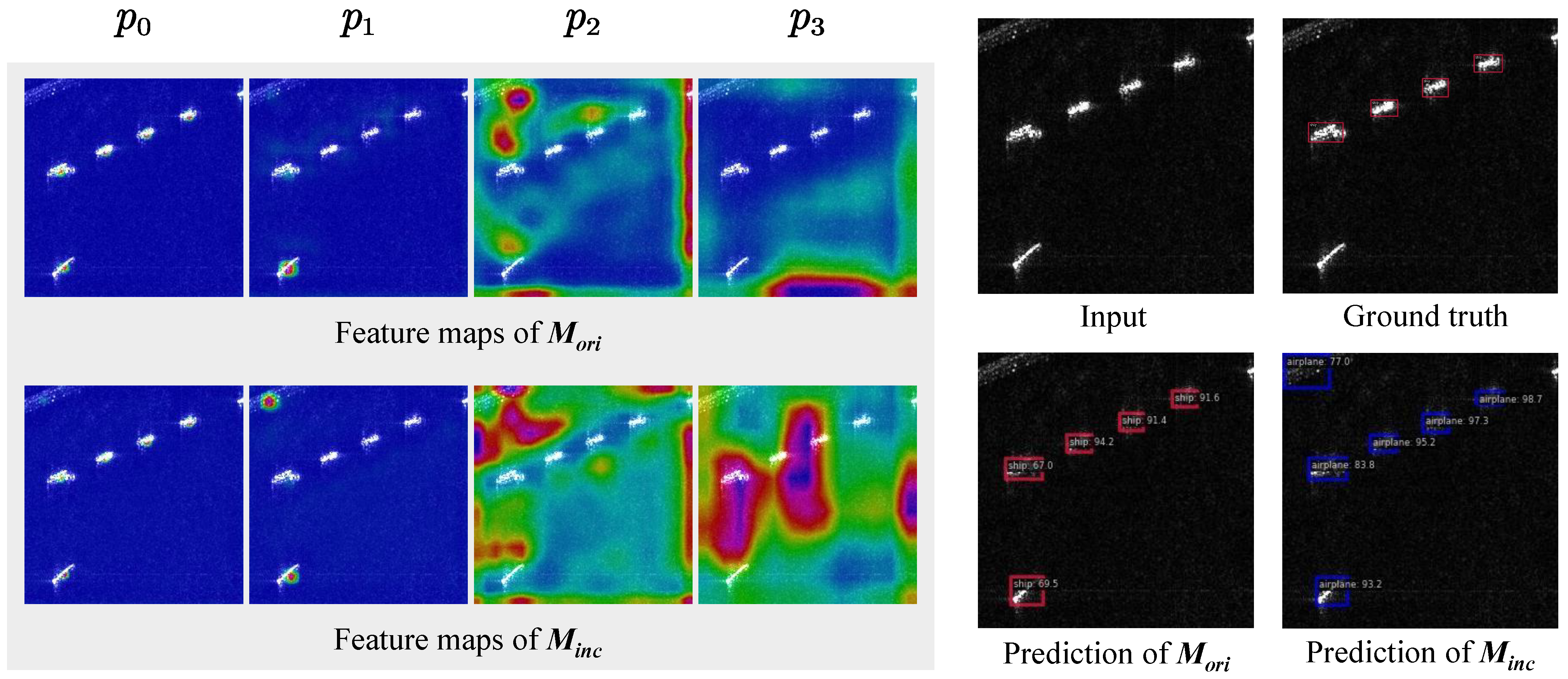
Figure 1. Comparison of features and detection results between the original model M o r i and the incremental model M i n c is presented. M o r i is trained using ship and bridge samples, while M i n c is incrementally trained on top of M o r i with additional oilcan and airplane data. The training follows the ERD method, and all samples are drawn from the MSAR [33] dataset. It is observed that M i n c ’s low-level features undergo unnecessary spatial shifts, while its deep features fail to focus on critical regions. Consequently, although target locations are detected, class prediction errors and false alarms occur.
Remotesensing 17 03214 g001
Figure 2. KD-based incremental target detection framework.
Remotesensing 17 03214 g002
Figure 3. Illustration of hierarchical feature maps and their DWT-based frequency decompositions. Row 1 (left → right): Spatial-domain feature maps at pyramid levels p 0 - p 3 . Row 2: For each level, the four frequency sub-bands are displayed as a L L L H H L H H (top-left: LL, top-right: LH, bottom-left: HL, bottom-right: HH). Each sub-band has half the spatial resolution per dimension (thus one quarter of the area) relative to the original feature map; therefore, we tile { LL , LH , HL , HH } to keep the panel size comparable across rows.
Remotesensing 17 03214 g003
Figure 4. A quantitative validation of the hierarchical-frequency correlation through Wasserstein Distance measurements across layers. The heatmap reveals that frequency-domain features, especially low-frequency ones, exhibit a higher degree of consistency across hierarchical levels compared to the original features. This finding forms the theoretical basis for the proposed HFKR strategy.
Remotesensing 17 03214 g004
Figure 5. Schematic diagram of the HFKR operational process. HFKR starts by extracting feature maps from the teacher ( M t ) and student ( M s ) models, then applying 2D wavelet decomposition to yield d w t 1 and d w t 2 . Their frequency components are cross-combined and reconstructed via inverse convolution to form F t s * and F s t * . Feature distillation follows to calculate loss. The gray-highlighted example shows M s adapting by shifting attention from targets to background, while the reconstructed feature maps re-establish the correlation between the underlying features and abstract features of the two models.
Remotesensing 17 03214 g005
Figure 6. Comparison of detection results across different combinations of λ and wavelet bases, based on the MSAR (2 + 2) data configuration.
Remotesensing 17 03214 g006
Figure 7. Qualitative comparison of detection results on the MSAR dataset. Each subfigure presents three sample results for a specific method. The proposed method (HFKR) achieves accurate and consistent detection performance, comparable to the full-data (FD) baseline and closer to the ground truth (GT) than other incremental learning approaches. (a) Ground Truth. (b) FD. (c) RILOD. (d) SID. (e) ERD. (f) IDCOD. (g) Tian. (h) Ours (HFKR). (To avoid occluding small and densely distributed targets, we remove in-image text labels for airplane and oilcan; blue boxes denote airplane, and light-purple boxes denote oilcan).
Remotesensing 17 03214 g007
Figure 8. Feature and detection evolution on the SARAIRcraft dataset across three incremental learning stages. Each row shows the shallow features (p0), deep features (p3), and detection output. (a) step 1. (b) step 2. (c) step 3.
Remotesensing 17 03214 g008
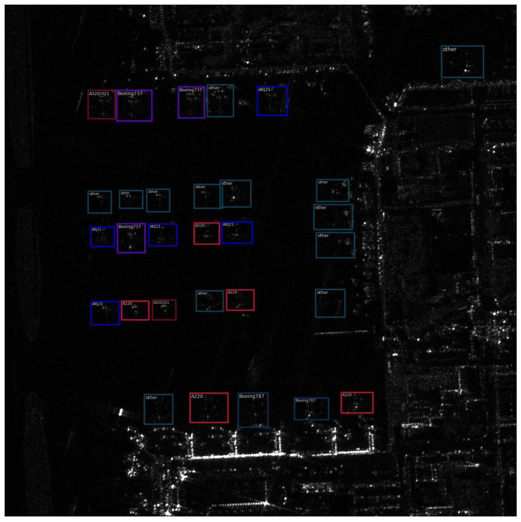
Figure 9. The ground truth of the detected image in Figure 8.
Remotesensing 17 03214 g009
Table 1. Information about the data.
MSARSARAIRcraft
SensorHS-1, GF-3GF-3
Wave Bandcc
Polarization Modemulti-polarizationsingle-polarization
Resolution1 m1 m
Image Size (pixels)256∼2048800∼1500
Number of Imagesship: 26,094
bridge: 1582
oilcan: 1248
airplane: 108
A220: 2065
A320/321: 939
A330: 290
ARJ21: 713
Boeing737: 1495
Boeing787: 1677
other: 2041
Number of Targetsship: 39,858
bridge: 1815
oilcan: 12,319
airplane: 6368
A220: 3730
A320/321: 1771
A330: 309
ARJ21: 1187
Boeing737: 2557
Boeing787: 2645
other: 5264
Table 2. Processed dataset.
Number of ImagesNumber of Targets
Ship30004838
Bridge15821815
Oilcan9508089
Airplane1086368
Table 3. Comparison of low-pass and high-pass filter coefficients for different wavelet bases.
Wavelet BasisLow-Pass Filter hHigh-Pass Filter g
haar (db1) 1 2 1 2 1 2 1 2
db2 1 + 3 4 2 3 + 3 4 2 3 3 4 2 1 3 4 2 3 1 4 2 3 3 4 2 3 + 3 4 2 1 + 3 4 2
coif2 h 0 h 1 h 11 ( 1 ) 0 h 11 ( 1 ) 1 h 10 ( 1 ) 11 h 0
Table 4. Performance comparison on MSAR (2 + 2) for with and without HFKR.
HFKRShipBridgeOilcanAirplaneAvg
73.5 (±0.2)73.4 (±0.4)93.1 (±0.1)43.6 (±0.1)70.9
73.7 (±0.1)71.6 (±0.2)97.3 (±0.2)58.9 (±0.6)75.4
Table 5. Performance comparison on MSAR Dataset.
PhaseMethodClassesmAPDiff (vs. FD)
ShipBridgeOilcanAirplaneOldNewAvgOldNewAvg
InitialFD (classes 1–2)79.584--------
Inc (2 + 2)FD (classes 1–4)79.180.697.460.979.879.279.5---
RILOD * (2019, SEC) [40]52.862.297.139.157.568.162.8−26.3−11.1−16.7
SID † (2021, CVPR) [24]73.179.789.84.476.445.161.7−3.4−34.1−17.8
ERD (2022, CVPR) [25]73.677.196.043.675.469.872.6−4.4−9.4−6.9
IDCOD * (2024, IJON) [42]65.071.097.758.668.078.273.1−11.8−1.0−6.4
Tian (2024, TGRS) [41]73.174.793.051.773.972.473.1−5.9−6.8−6.4
Ours73.771.697.358.972.778.175.4−7.1−1.1−4.1
Table 6. Performance comparison on SARAIRcraft dataset (A22: A220, A32: A320/321, A33: A330, ARJ: ARJ21, B73: Boeing737, B78: Boeing787).
PhaseMethodClassesmAPDiff (vs. FD)
A22A32A33ARJB73B78OtherOldNewAvgOldNewAvg
InitialFD (classes 1–2)62.378.2-----------
Inc (2 + 2)FD (classes 1–4)63.986.078.074.8---74.976.475.7---
RILOD * (2019, SEC) [40]50.068.473.160.0 --59.266.662.9−15.7−9.8−12.8
SID † (2021, CVPR) [24]54.981.077.059.3---67.968.268.2−7.0−8.2−7.5
ERD (2022, CVPR) [25]56.680.961.462.0---68.861.765.2−6.1−14.7−10.2
IDCOD * (2024, IJON) [42]32.356.976.458.8---44.667.656.1−30.3−8.8−19.6
Tian (2024, TGRS) [41]50.871.877.264.2---61.370.765.8−13.6−5.7−9.9
Ours62.081.675.566.7---71.871.171.4−3.1−5.3−4.3
Inc (4 + 2)FD (classes 1–6)57.893.977.268.464.177.8-74.371.073.2---
RILOD * (2019, SEC) [40]43.177.958.546.551.273.0-56.562.158.4−17.8−8.9−14.8
SID † (2021, CVPR) [24]53.986.979.571.852.663.3-73.057.968.0−1.3−13.1−5.2
ERD (2022, CVPR) [25]56.887.578.075.653.158.9-74.556.068.3+0.2−15.0−4.9
IDCOD * (2024, IJON) [42]44.382.268.854.461.672.2-62.466.963.9−11.9−4.1−9.3
Tian (2024, TGRS) [41]50.284.579.164.761.070.7-72.665.968.4−1.7−5.1−4.8
Ours52.087.977.275.056.874.3-73.065.670.5−1.3−5.4−2.7
Inc (6 + 2)FD (classes 1–7)66.989.877.281.265.477.479.476.379.476.8---
RILOD * (2019, SEC) [40]40.386.276.968.854.169.370.465.970.466.6−4.5−9.0−10.2
SID † (2021, CVPR) [24]57.190.977.273.962.678.270.073.370.072.8−3.0−9.4−4.0
ERD (2022, CVPR) [25]59.294.577.272.364.377.866.074.166.073.0−2.2−13.4−3.4
IDCOD * (2024, IJON) [42]41.384.658.367.646.352.874.958.574.960.8−17.8−4.5−16.0
Tian (2024, TGRS) [41]41.987.277.269.956.371.873.167.473.168.2−8.9−6.3−8.6
Ours58.093.977.273.862.478.074.873.974.874.0−2.4−4.6−2.8
Disclaimer/Publisher’s Note: The statements, opinions and data contained in all publications are solely those of the individual author(s) and contributor(s) and not of MDPI and/or the editor(s). MDPI and/or the editor(s) disclaim responsibility for any injury to people or property resulting from any ideas, methods, instructions or products referred to in the content.