ESA-MDN: An Ensemble Self-Attention Enhanced Mixture Density Framework for UAV Multispectral Water Quality Parameter Retrieval

Highlights

What are the main findings?

• An ESA-MDN model is proposed to achieve high-precision modeling of the probability distribution of water quality parameters.
• Data augmentation is accomplished by leveraging the relationship between “multi-point sampling mean and multi-pixel reflectance”, thereby resolving the issue of insufficient sample size.

What is the implication of the main finding?

• ESA-MDN effectively extracts water quality parameters from multispectral data, enabling the generation of spatiotemporal maps critical for identifying pollution sources and guiding emergency responses.
• Data augmentation can effectively increase the sample size, thereby providing more possibilities for improving model accuracy.

Abstract

Urban rivers, as crucial components of ecosystems, serve multiple functions, including flood control, drainage, and landscape services. However, with the acceleration of urbanization, factors such as industrial wastewater discharge, domestic sewage leakage, and surface runoff pollution have led to increasingly severe degradation of water quality in urban rivers. Unmanned aerial vehicle (UAV) remote sensing technology, with its sub-meter spatial resolution and operational flexibility, demonstrates significant advantages in the detailed monitoring of complex urban water systems. This study proposes an Ensemble Self-Attention Enhanced Mixture Density Network (ESA-MDN), which integrate an ensemble learning framework with a mixture density network and incorporates a self-attention mechanism for feature enhancement. This approach better captures the nonlinear relationships between water quality parameters and remote sensing features, achieving high-precision modeling of water quality parameter distributions. The resulting spatiotemporal distribution maps provide valuable support for pollution source identification and management decision making. The model successfully retrieved five water quality parameters, Chl-a, TSS, COD, TP, and DO, and validation metrics such as R², RMSE, MAE, MSE, MAPE, bias, and slope were utilized. Key metrics for the ESA-MDN test set were as follows: Chl-a (R² = 0.98, RMSE = 0.31), TSS (R² = 0.93, RMSE = 0.27), COD (R² = 0.93, RMSE = 0.39), TP (R² = 0.99, RMSE = 0.02), and DO (R² = 0.88, RMSE = 0.1). The results indicated that ESA-MDN can effectively extract water quality parameters from multispectral remote sensing data, with the generated spatiotemporal water quality distribution maps providing crucial support for pollution source identification and emergency response decision making.

1. Introduction

Urban rivers, as vital components of ecosystems, not only fulfill flood control and landscape recreation functions but also serve as critical indicators of urban aquatic environmental health [1,2]. However, accelerated urbanization has led to persistent water quality deterioration under combined pressures from industrial wastewater, domestic sewage, and surface runoff pollution [3,4], creating an urgent demand for rapid, large-scale water quality monitoring in environmental governance. Remote sensing technology, with its advantages of extensive spatial coverage and periodic monitoring, compensates for the limitations of traditional sampling methods. It enables the spatiotemporal dynamic monitoring of water quality parameters, thereby providing significant technical support for global water environment management and achievement of the United Nations’ Sustainable Development Goals (SDGs). While satellite remote sensing offers broad-scale observational capabilities, it is constrained by spatial resolution limitations. By contrast, unmanned aerial vehicle (UAV)-based remote sensing achieves high-frequency, refined monitoring of urban small rivers through sub-meter resolution and operational flexibility [5,6]. Regarding the choice between hyperspectral and multispectral systems, the former remains predominant in water quality remote sensing research, yet its high costs and reliance on heavy-duty UAVs (>5 kg) significantly constrain its widespread adoption. The latter demonstrates superior engineering practicality owing to cost-effectiveness, lightweight design, and operational efficiency [7,8].

Both hyperspectral and multispectral water quality inversion fundamentally rely on the optical properties of aquatic constituents—distinct substances exhibit unique absorption-scattering characteristics at specific wavelengths due to variations in molecular structure and particle size, enabling quantitative concentration monitoring through inversion model development [9,10]. Accurately characterizing the response mechanisms of spectral reflectance to water quality parameters remains the central challenge in aquatic remote sensing research [11,12,13].

Optically active substances, such as chlorophyll-a (Chl-a) and total suspended solids (TSS), exhibit distinct optical response characteristics in specific spectral bands, enabling precise inversion through characteristic band analysis [14,15,16,17]. By contrast, non-optically active parameters, including chemical oxygen demand (COD), total phosphorus (TP), and dissolved oxygen (DO), lack direct spectral response properties, making them challenging to detect directly via remote sensing. However, their concentration variations often demonstrate significant correlations with band combination results, providing potential for indirect estimation [18]. Therefore, this study aims to achieve the inversion of Chl-a, TSS, COD, TP, and DO through algorithmic modeling.

Traditional water quality remote sensing inversion methods employ empirical/semi-analytical models constructed through characteristic band selection and multiple regression analysis. However, such models generally suffer from limited generalization capabilities [19,20,21]. The breakthrough of artificial intelligence technology has introduced novel paradigms for remote sensing data processing [22]. Its adaptive learning capacity effectively addresses nonlinear modeling challenges with multi-source heterogeneous remote sensing data, demonstrating remarkable advantages in enhancing the inversion accuracy of water quality parameters [23,24]. Research indicates that machine learning methods significantly outperform traditional methods in the inversion of water quality parameters [25,26]. However, traditional machine learning approaches have limitations when handling multispectral data, as these data possess fewer spectral channels, resulting in restricted feature representation capabilities. Moreover, they lack sufficient flexibility in addressing nonlinear problems, which may lead to overlooking the complex nonlinear relationships between spectral features and water quality parameters, resulting in overfitting or underfitting phenomena. Consequently, scholars have proposed ensemble learning methods that improve model performance in terms of accuracy and robustness through combination strategies, leading to better outcomes [27,28]. Deep learning, with its capability for multi-level automatic feature extraction, demonstrates a powerful advantage in representation learning when handling high-dimensional nonlinear water quality data. Combined with its end-to-end modeling characteristics, it has become the core algorithm in current water quality remote sensing research [29,30].

In summary, current water quality remote sensing inversion using multispectral data has two major limitations: (1) compared to hyperspectral data, multispectral data, with a limited number of bands, show weaker spectral representation capabilities, resulting in significant gaps in modeling accuracy and applicability for complex water quality parameter inversion; and (2) traditional empirical algorithms and conventional machine learning methods demonstrate insufficient ability to extract and characterize nonlinear features from multispectral data, making it difficult to capture the complex nonlinear response relationships between water constituents and multispectral reflectance, which leads to generally lower inversion accuracy than hyperspectral methods. To address these issues, this study integrates an ensemble learning framework with a mixture density network, proposing an Ensemble Self-attention Augmented Mixture Density Network (ESA-MDN) model tailored for UAV multispectral imagery, enabling the inversion of Chl-a, TSS, COD, TP, and DO in urban small rivers. The model offers several advantages: (1) it features strong hierarchical representation of features and enhanced transferability, effectively improving the inversion accuracy and cross-scenario generalization capability for urban river network water quality monitoring; and (2) the incorporation of a self-attention mechanism enhances feature interactions across bands, allowing for deep extraction of information from limited spectral channels, achieving inversion accuracy comparable to that of hyperspectral data. The significance of this research lies in its innovative integration of ensemble learning and deep learning, which fully demonstrates the potential of multispectral remote sensing technology in environmental monitoring, thereby providing critical technical support for rapid and precise monitoring of global water environments and effectively promoting the collaborative achievement of water ecological management and sustainable development goals.

2. Materials and Methods

The experimental workflow comprised five key steps: (1) Selection of the study area: a typical urban river network is selected as the research area. (2) UAV image acquisition and preprocessing: multispectral remote sensing images were obtained using a DJI M300 RTK drone, followed by radiometric correction, geometric correction, and image mosaicking. (3) Water quality data collection and preprocessing: water samples were collected and analyzed for Chl-a, TSS, COD, TP, and DO parameters according to the GB3838-2002 standard [31], with subsequent data augmentation. (4) Correlation analysis between water quality parameters and spectral reflectance: Pearson correlation coefficients were employed to analyze the response relationships between various band combinations and Chl-a, TSS, COD, TP, and DO, identifying sensitive characteristic bands for inversion model construction. (5) Model development: the ESA-MDN model was established and compared against six representative machine learning models for validation. (6) Model accuracy evaluation: the dataset was randomly split into training and testing sets at an 8:2 ratio, with seven metrics systematically assessing the inversion accuracy and consistency for five water quality parameters (Chl-a, TSS, COD, TP, and DO).

2.1. Study Area

The study area selected was the Lianqi River in Jiading District and Baoshan District of Shanghai (121°21′13″ E–121°21′38″ E, 31°24′34″ N–31°25′42″ N). As the main waterway in the northern Jiading–Baoshan area, the Lianqi River serves multiple functions, including flood control, drainage, shipping, and water diversion, and it is capable of accommodating ships up to 100 tons. The research area was centered along the central line of the Lianqi River, covering typical river water bodies and adjacent ecosystems, making it an ideal location for studying the water environmental characteristics of urban river networks. The surveyed area extended along the central axis of the Lianqi River, with a length of 3.7 km, a width of 0.8 km, and a total area of 2.96 km², as shown in Figure 1.

2.2. UAV Imagery Acquisition and Preprocessing

Data collection was completed in the experimental area using the DJI M300 UAV equipped with the Chang Guang Yu Chen AQ600 Pro multispectral camera, with the parameters provided in

Table 1. Basic information table for UAV flight.

Basic Information on Multispectral Data
Collection Time	8 October 2024 10:00–16:00	Spatial Resolution	10 cm
UAV Flight Height	110 m	UAV Flight Frequency	11
On-site Wind Force	2–3	Weather Conditions	Clear and cloudless weather

. This multispectral camera includes five spectral lenses, with central wavelengths and bandwidths of 450 nm ± 15 nm, 555 nm ± 13.5 nm, 660 nm ± 11 nm, 720 nm ± 5 nm, and 840 nm ± 15 nm, respectively. The field of view is 48.8° × 37.5°. The raw data obtained after the flight was in radiance value format. Before the flight, a calibration plate was photographed using the UAV; this calibration plate was used to convert the DN values of the multispectral images to reflectance. The collected data underwent preprocessing steps, including geometric correction, image stitching, and reflectance calculation, to obtain the surface reflectance data. The relationship between remote sensing reflectance and radiance values for each band is expressed as follows:

R_rs = a_i × L_i + b_i

(1)

For the i-th spectral band, a_i and b_i denote the calibration coefficients, where R_rs represents the corrected reflectance and L_i corresponds to the radiance value.

2.3. Water Quality Data Collection and Preprocessing

This experiment achieved comprehensive data collection through a combination of UAV multispectral photogrammetry and synchronized ground sampling. A total of 30 sampling points were systematically established within the study area (Figure 1c), and water samples were collected at a depth of 20 cm below the water surface using a sampler with a diameter of 30 cm. Each sampling point covered a circular area with a radius of 35 cm and five replicates were collected (Figure 2). The samples were then transferred to a mixing container for homogenization, resulting in a 3 L mixed sample stored in brown glass bottles protected from light until laboratory analysis. Sampling coordinates were recorded using a high-precision GPS, and the determination of water quality parameters (Chl-a, TSS, COD, TP, and DO) strictly followed the GB3838-2002 standard.

Table 2. Basic information on the five water quality parameters.

	Chl-a	TSS	COD	TP	DO
Max	10	9	15	0.95	5.81
Min	2	6	9	0.06	4.2
Mean	4.33	7.73	11.87	0.17	4.95
SD	2.01	1.01	1.53	0.17	0.29

presents the statistical analysis results for the different indicators.

The spatial resolution of the UAV images was 10 cm, and each water quality sampling result represents the average of five samples within a 35 cm radius. Considering the minimal water quality variations over small spatial scales, a circular buffer with a radius of 35 cm was created around each sampling coordinate. Within this circular buffer, the reflectance of the center pixel and nine randomly distributed pixels was extracted (Figure 2). A total of 300 data points were collected, consisting of 30 center points and 270 random points. To ensure data validity, if any outlier reflectance values were detected within the randomly sampled points (exceeding the mean ± 3 standard deviations of adjacent pixels), they were replaced with qualified pixels that had a spectral similarity greater than 90% within a neighboring buffer zone (≤15 cm). Given the sub-meter spatial homogeneity characteristics of river water quality, the reflectance values of the ten pixels within the circular buffer were matched with the corresponding field measurements. This approach effectively reduced positional errors while fully leveraging the spatial information from UAV imagery to enhance the quality of point data.

2.4. Correlation Analysis Between Water Quality Parameters and Spectral Reflectance Values

This study conducted systematic band combination analysis (

Table 3. Band operation rules table.

Type	Band Combination Formulas
Dual-band Combinations	B1 + B2	(B1 + B2)/B2	e(B1 + B2) × B1
	B1 − B2	B1/(B1 − B2)	e(B1 + B2) × B2
	B1 × B2	B2/(B1 − B2)	e(B1 − B2)/B1
	B1/B2	B1/(B1 + B2)	e(B1 − B2)/B2
	(B1 − B2)/(B1 + B2)	B2/(B1 + B2)	e(B1 + B2)/B1
	((B1)2 − (B2)2)/((B1)2 + (B2)2)	eB1 + B2	e(B1 + B2)/B2
	(B1 − B2) × B1	eB1 − B2	e B1/(B1 − B2)
	(B1 − B2) × B2	eB1 × B2	e B2/(B1 − B2)
	(B1 + B2) × B1	eB1/B2	e B1/(B1 + B2)
	(B1 + B2) × B2	e(B1 − B2)/(B1 + B2)	e B2/(B1 + B2)
	(B1 − B2)/B1	$e^{({(B1)}^2-{(B2)}^2)/({(B1)}^2+{(B2)}^2)}$	Log10(1/B1)
	(B1 − B2)/B2	e(B1 − B2) × B1	Log10(1/B1) − Log10(1/B2)
	(B1 + B2)/B1	e(B1 − B2) × B2	Log10(1/B1) + Log10(1/B2)
Three-band combinations	B1 + B2 + B3	(B1 − B2) × B3	e B1 × B2 × B3
	B1 + B2 − B3	B1/(B2 + B3)	e (B1 − B2)/B3
	(B1 − B2 + B3)/(B1 + B2 + B3)	B1/(B2 − B3)	e (B1 + B2) × B3
	(B1 − B2 + B3)/(B1 + B2 − B3)	e B1 + B2 + B3	e (B1 − B2) × B3
	(B1 × B2)/B3	e B1 + B2 − B3	e B1/(B2 + B3)
	(B1 + B2)/B3	e (B1 − B2 + B3)/(B1 + B2 + B3)	e B1/(B2 − B3)
	B1 × B2 × B3	e (B1 − B2 + B3)/(B1 + B2 − B3)	Log10(1/B1) + Log10(1/B2) + Log10(1/B3)
	(B1 − B2)/B3	e (B1 × B2)/B3	Log10(1/B1) − Log10(1/B2) − Log10(1/B3)
	(B1 + B2) × B3	e (B1 + B2)/B3	Log10(1/B1) − Log10(1/B2) + Log10(1/B3)

) using five-band (B1–B5) UAV multispectral imagery to calculate Pearson correlation coefficient matrices between spectral feature variables and water quality parameters (Chl-a, TSS, COD, TP, and DO), thereby enhancing the inversion accuracy of water quality parameters.

2.5. Ensemble Self-Attention Enhanced Mixture Density Networks (ESA-MDN) Learning Model

This study addresses the complex distribution characteristics and uncertainty quantification challenges of urban water quality by proposing an Ensemble Self-Attention Enhanced Mixture Density Network (ESA-MDN) architecture (Figure 3). The model combines the feature engineering capability of machine learning, the nonlinear representation ability of deep learning, and the uncertainty quantification advantage of probabilistic modeling to achieve end-to-end probabilistic prediction.

The Mixture Density Network (MDN) represents a class of deep learning models that integrate neural networks with probabilistic modeling, specifically designed to address the limitations of conventional regression models in handling multimodal output distributions. This capability proves particularly critical in water quality modeling, where complex distribution patterns emerge from: (i) composite effects of mixed pollution sources (e.g., superposition of point-source discharges and agricultural runoff), (ii) periodic hydrodynamic processes (e.g., concentration fluctuations induced by tidal cycles), and (iii) spatiotemporal heterogeneity in biogeochemical reactions (e.g., patchy distribution of algal blooms). These mechanisms frequently generate bimodal or multimodal distributions that MDNs capture through full probability distribution outputs. The model assumes that the target variable y follows a Gaussian Mixture Model (GMM), mathematically expressed as a weighted combination of K Gaussian components with the conditional probability distribution:

$$P(y| x)={\displaystyle \sum _{k=1}^K{\pi }_k(x)}·N(y| {\mu }_k(x),{{\sigma }_k}^2(x))$$

(2)

where K denotes the number of Gaussian components in the mixture model, while π_k(x) represents the mixture weight coefficient corresponding to the k-th Gaussian distribution, which quantifies the relative importance of this component given the input vector x. The probability density function of the k-th Gaussian component is given by $N(y| {\mu }_k(x),{{\sigma }_k}^2(x))$, where μ_k(x) represents the conditional mean of this distribution mode and σ_k(x) quantifies its standard deviation as a measure of uncertainty, as formally defined in Equation (3):

$$N(y| \mu ,{\sigma }^2)={\displaystyle \frac{1}{\sqrt{2\pi {\sigma }^2}}}exp(-{\displaystyle \frac{{(y-\mu )}^2}{2{\sigma }^2}})$$

(3)

$$\begin{array}{l}{\mu }_k=W_{\mu }h+b_{\mu }\begin{array}{cc} & ,\end{array}{\sigma }_k=\mathit{softplus}(W_{\sigma }h+b_{\sigma })\\ \mathit{softplus}(z)=log(1+e^z)\end{array}$$

where W_μ denotes the weight matrix of the mean prediction layer, h represents the feature vector output from the backbone network, and b_μ corresponds to the bias term of the mean prediction layer. Similarly, W_σ signifies the weight matrix of the standard deviation prediction layer, where the softplus activation function ensures the positivity constraint of the standard deviation, and b_σ indicates the bias term of the standard deviation prediction layer.

While Mixture Density Networks (MDNs) provide an innovative probabilistic solution for water quality parameter inversion, they face significant challenges in urban water monitoring applications: (1) limited spectral bands in multispectral imagery constrain the feature representation capacity of conventional MDNs, hindering their ability to extract latent feature information; and (2) training instability and mode collapse frequently occur due to the multimodal nature of likelihood functions. These limitations substantially restrict MDN applications in complex urban aquatic environments. To address these issues, we developed an Enhanced Self-attention MDN (ESA-MDN) that incorporates: (i) ensemble learning-based multimodal inputs, (ii) hierarchical input-network/backbone-network architecture, (iii) self-attention enhanced feature extraction, (iv) regularized mixture density loss functions, and (v) dynamic early stopping mechanisms to prevent overfitting—collectively establishing a robust framework for urban water quality monitoring.

To construct multimodal input features through ensemble learning while addressing the computational challenges posed by large-scale UAV datasets, we employ a dimensionality-reduction strategy that maintains inversion accuracy of water quality parameters. This approach utilizes prediction outputs from four heterogeneous models (CatBoost, KNN, Random Forest, and XGBoost) as integrated inputs to enhance feature representation capacity. The ensemble framework leverages complementary strengths: (i) CatBoost’s ordered boosting algorithm optimally handles categorical features in spectral data, (ii) XGBoost’s second-order Taylor expansion-based gradient boosting framework captures nonlinear band interactions, (iii) Random Forest demonstrates superior small-sample adaptability for feature stability preservation, and (iv) KNN’s distance-based modeling effectively represents spatial autocorrelation through buffered random sampling of aquatic data points.

The ESA-MDN architecture employs a hierarchical input-network/backbone-network design that significantly enhances both feature representation capacity and multimodal modeling precision for water quality inversion. The input network implements high-dimensional mapping with strong regularization, transforming raw inputs into discriminative features while effectively suppressing noise interference. The backbone network integrates: (i) a self-attention mechanism to capture global interdependencies among bands, and (ii) a bottleneck structure (compressing features to hidden_dim//2) to enforce focus on the most discriminative characteristics.

The conventional MDN employs fully-connected layers for direct mixture parameter estimation, which fails to effectively capture long-range dependencies among bands. To address this limitation, we introduce a multi-head self-attention mechanism that computes parallel projections of Query (Q), Key (K), and Value (V) matrices, enabling simultaneous modeling of synergistic variations across different band combinations, as formulated in Equation (4):

$$\begin{array}{l}hea{d}_i=\mathit{softmax}(({\displaystyle \frac{Q_i{K_i}^T}{\sqrt{d_k}}})V_i)\\ Q=X{W}_Q\hspace{1em}, K=X{W}_K\hspace{1em}, V=X{W}_V\end{array}$$

(4)

where X represents the input feature matrix, with W_Q, W_K, and W_V denoting the projection weight matrices for Query (Q), Key (K), and Value (V), respectively. To further enhance the accuracy and stability of water quality parameter inversion, the architecture incorporates residual connections and layer normalization, effectively addressing gradient vanishing issues while improving dynamic adaptation capabilities, as computed in the following equation:

$$\begin{array}{l}{h}_{mid}=LayerNorm(h_{in}+MultiHead(h_{in}))\\ h_{out}=LayerNorm(h_{mid}+FFN(h_{mid}))\end{array}$$

(5)

where h_in denotes the input features, MultiHead(h_in) represents the output of multi-head attention, LayerNorm signifies layer normalization, h_mid corresponds to the intermediate features after the first residual connection, and FFN indicates the feed-forward network.

The regularized mixture density loss function is optimized through the collaborative integration of three core components: negative log-likelihood loss, entropy regularization term, and variance constraint term. Its primary advantage lies in the dual assurance of probabilistic output and dynamic regularization mechanism, which simultaneously enhances predictive accuracy and model robustness. The negative log-likelihood loss serves as the essential component for ensuring prediction accuracy; by minimizing this loss, the distribution predicted by the model approximates the actual distribution of the real data as closely as possible. The entropy regularization term prevents mode collapse by maintaining an appropriate contribution ratio among different factors. The variance constraint effectively mitigates overfitting and gradient anomalies by balancing predictive uncertainty. This integrated approach ultimately achieves a more accurate modeling of the distribution of water quality parameters, mathematically expressed as follows:

$$\mathcal{L}=\underset{\mathrm{NLL} \mathrm{Loss}}{\underbrace{-\mathbb{E}\left[\log {\displaystyle \sum _{k=1}^K{\pi }_k}\mathcal{N}\left(y| {\mu }_k,{\sigma }_k\right)\right]}}+\underset{\mathrm{Entropy} \mathrm{Regularization} \mathrm{Term}}{\underbrace{\alpha \mathbb{E}\left[-{\displaystyle \sum _{k=1}^K{\pi }_k}\log {\pi }_k\right]}}+\underset{\mathrm{Variance} \mathrm{Constraint}}{\underbrace{\beta \mathbb{E}\left[{\displaystyle \frac{1}{\sigma }}+\sigma \right]}}$$

(6)

where y represents the true observed value, μ_k is the mean value, and σ_k is the standard deviation. The term ${\displaystyle \sum _{k=1}^K}$π_kN(y∣μ_k,σ_k) indicates the mixture model where the probabilities are weighted by π_k, leading to the overall likelihood of being generated by the mixture of Gaussian distributions. αα denotes the regularization parameter, and −∑π_klogπ_k is the entropy of the calculation. β represents the regularization factor, which prevents the standard deviations of the Gaussian components (σ) from manifesting extreme values (either too large or too small), thereby averting uncertainty in the measurement. The complete ESA-MDN model architecture is then established by incorporating a dynamic early-stopping mechanism.

To systematically evaluate the performance advantages of the ESA-MDN model, this study selects six representative baseline algorithms encompassing diverse paradigms, including ensemble learning, distance metrics, and neural networks: CatBoost, KNN, Random Forest (RF), XGBoost, LightGBM, and Multilayer Perceptron (MLP). All comparative models underwent automated hyperparameter optimization via Bayesian optimization to ensure fair comparisons under optimal configurations. This benchmark testing framework was meticulously designed to incorporate methodological diversity and representativeness, thereby providing a comprehensive and reliable reference system for model performance assessment.

2.6. Model Accuracy Evaluation

The dataset was randomly divided into training and testing sets at an 8:2 ratio, resulting in a total of 240 samples in the training set and 60 samples in the testing set. The model performance for five key water quality parameters (Chl-a, TSS, COD, TP, and DO) was systematically evaluated using seven metrics: coefficient of determination (R²), root mean square error (RMSE), mean absolute error (MAE), mean square error (MSE), mean absolute percentage error (MAPE), bias, and linear regression slope. This multidimensional assessment framework provided a comprehensive quantification of prediction accuracy and consistency for all measured parameters, as detailed in Equation (7):

$$\begin{array}{l}{R}^2=1-{\displaystyle \frac{{\displaystyle \sum {\left(y_i-{\widehat{y}}_i\right)}^2}}{{\displaystyle \sum {\left(y_i-\overline{y}\right)}^2}}}\\ RMSE=\sqrt{{\displaystyle \frac{1}{n}}{\displaystyle \sum _{i=1}^n{\left({\widehat{y}}_i-y_i\right)}^2}}\end{array}\hspace{1em}\begin{array}{l}MAE={\displaystyle \frac{1}{n}}{\displaystyle \sum _{i=1}^n\left|{\widehat{y}}_i-y_i\right|}\\ MAPE={\displaystyle \frac{100\%}{n}}{\displaystyle \sum _{i=1}^n\left|\frac{y_i-{\widehat{y}}_i}{y_i}\right|}\end{array}\hspace{1em}\begin{array}{l}bias={\displaystyle \frac{1}{n}}{\displaystyle \sum _{i=1}^n\left(y_i-{\overline{y}}_i\right)}\\ Slope={\displaystyle \frac{{\displaystyle \sum _{i=1}^n\left(y_i-{\overline{y}}_i\right)}\left({\widehat{y}}_i-\overline{y}\right)}{{\displaystyle \sum _{i=1}^n{\left(y_i-{\overline{y}}_i\right)}^2}}}\end{array}$$

(7)

where n represents the sample size, y_i denotes the measured value of the water quality parameter, $\widehat{y}$_i corresponds to the predicted value of the water quality parameter, $\overline{y}$_i indicates the mean of measured values, and $\overline{y}$ is the mean of the predicted values.

3. Results

3.1. Band Combinations and Water Quality Parameters Selection

Through correlation analysis, a total of 2880 correlation coefficients were obtained for each water quality parameter. From these results, we excluded statistically insignificant, weakly correlated, and numerically unstable feature bands (such as those affected by overflow or invalid values). Ultimately, the top five optimal band combinations with the highest correlation to each water quality parameter were selected as model input variables. The feature bands used for modeling different water quality parameters, along with their corresponding correlation and significance results, are presented in

Table 4. Feature band selection and correlation analysis.

Feature Bands	Type	Chl-a	TSS	COD	TP	DO
X1	Band operation formula	Log10(1/B2) − Log10(1/B4) + Log10(1/B2)	B4 − B2	B5/(B1 − B3)	B2/(B4 − B3)	(B1 + B4)/B5
	Correlation coefficient	0.38	0.42	0.31	0.70	0.31
	p-value	5.17 × 10−7	1.38 × 10−12	2.84 × 10−7	2.30 × 10−31	2.48 × 10−6
X2	Band operation formula	Log10(1/B2) − Log10(1/B4) + Log10(1/B3)	(B1 − B2 + B4)/(B1 + B2 + B4)	B2/(B1 − B3)	B1/(B4 − B3)	(B4 − B5 + B1)/(B4 + B5 − B2)
	Correlation coefficient	0.37	0.38	0.31	0.70	0.31
	p-value	9.48 × 10−10	2.68 × 10−9	6.66 × 10−7	2.45 × 10−29	7.39 × 10−3
X3	Band operation formula	B1/(B4 − B3)	(B1 + B4)/B2	B4/(B1 − B3)	B5/(B4 − B3)	(B2 − B5 + B4)/(B2 + B5 − B4)
	Correlation coefficient	0.36	0.37	0.30	0.67	0.31
	p-value	1.34 × 10−9	1.18 × 10−10	8.05 × 10−7	4.57 × 10−27	2.86 × 10−3
X4	Band operation formula	Log10(1/B2) − Log10(1/B3) + Log10(1/B2)	(B5 − B1) × B1	B1/(B1 − B3)	B4/(B4 − B3)	(B3 − B5 + B1)/(B3 + B5 − B1)
	Correlation coefficient	0.35	0.37	0.29	0.66	0.31
	p-value	9.55 × 10−7	2.78 × 10−9	2.78 × 10−6	4.40 × 10−26	6.12 × 10−4
X5	Band operation formula	B5/(B4 − B3)	(B5 − B1) × B3	B3/(B4 − B1)	B4/(B3 − B1)	(B3 − B5 + B2)/(B3 + B5 − B2)
	Correlation coefficient	0.35	0.37	0.29	0.38	0.30
	p-value	5.35 × 10−11	2.40 × 10−9	4.21 × 10−6	2.30 × 10−11	2.37 × 10−3

.

3.2. Chl-a Model Performance Analysis

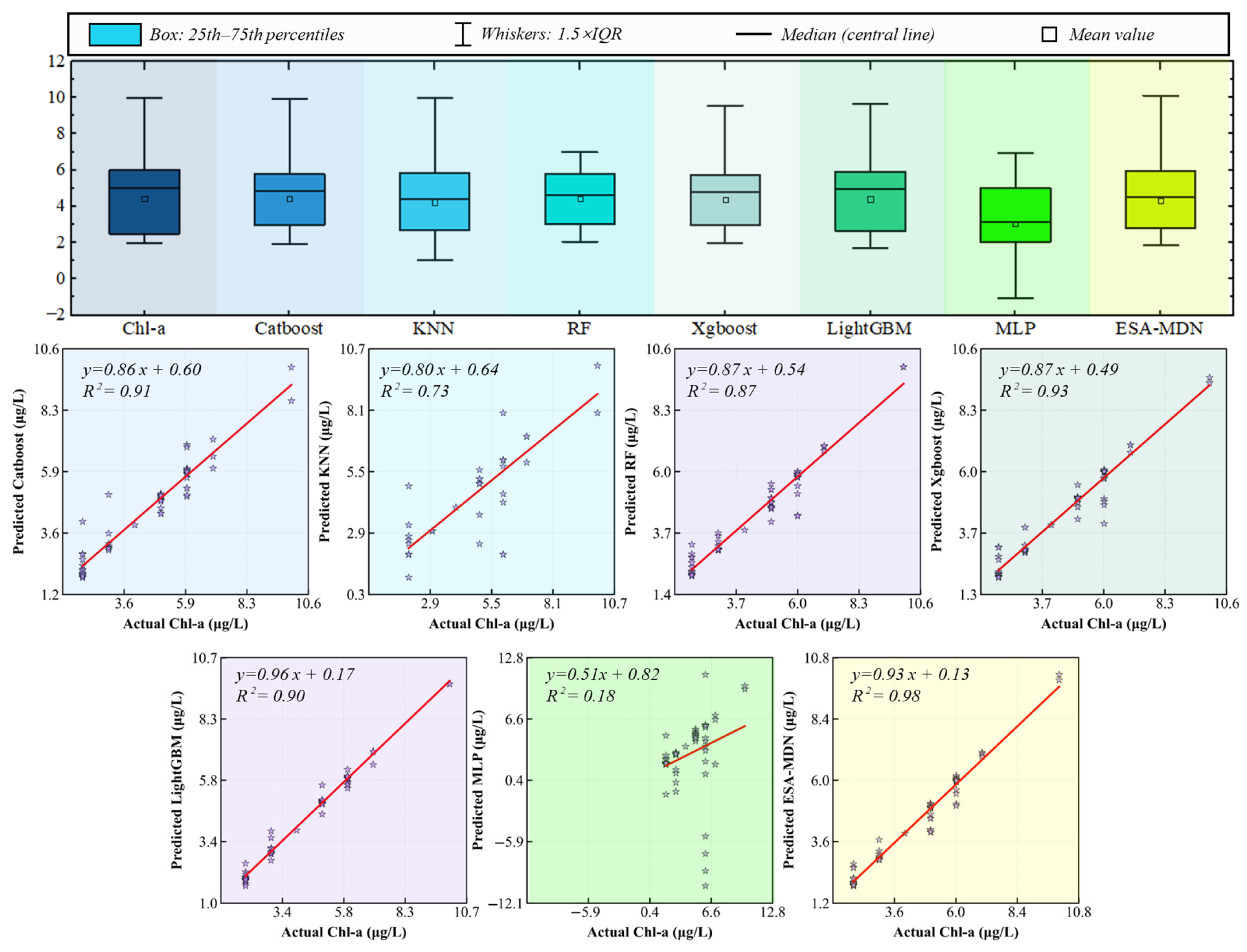
Based on the evaluation of chlorophyll-a concentration prediction performance with the test set (Figure 4), the box plot reveals significant differences in the distribution of prediction values across models. The MLP model exhibits a broader deviation from the actual data, while the ESA-MDN ensemble model demonstrates superior performance, with a coefficient of determination (R² = 0.98) for the predicted values significantly better than that of the other models.

Through systematic evaluation of seven models for chlorophyll-a (Chl-a) concentration retrieval, this study demonstrates that ESA-MDN exhibits significant advantages in both prediction accuracy and stability. The model achieves outstanding test set performance, with R² = 0.98, RMSE = 0.31, MAE = 0.21, MAPE = 6.80%, bias = −0.06, and near-optimal slope = 0.93, while showing minimal discrepancy between training and testing errors. These results confirm its superior generalization capability and effective resistance to overfitting (Figure 5). Among other machine learning models, XGBoost performs best with test set R² = 0.93, RMSE = 0.53, and MAPE = 10.54%. By contrast, the MLP model shows the poorest performance across all metrics, with critically low R² = 0.18, excessively high MAPE = 45.72%, and severe underestimation (Bias = −0.64). Compared with other algorithms, ESA-MDN maintains balanced performance across all evaluation metrics while demonstrating high sensitivity and stability, ensuring more reliable retrieval results. These characteristics make it particularly valuable for aquatic environment Chl-a monitoring applications.

3.3. TSS Model Performance Analysis

Figure 6 presents the results of TSS concentration from multiple models on the test set. In the box plot, most models, except for MLP, exhibit interquartile ranges (IQRs) concentrated near the actual values. The positioning of the ESA-MDN box and the whisker lengths align more closely with the true values, suggesting that the ensemble method may outperform individual models. In the scatter plot, ESA-MDN maintains a high coefficient of determination (R² = 0.93) while demonstrating a more stable predictive distribution.

The TSS concentration inversion results demonstrate that ESA-MDN exhibits optimal performance across all evaluation metrics. The model achieves superior test set performance, with R² = 0.93, RMSE = 0.27, MAE = 0.161, MSE = 0.07, and MAPE = 2.12%, significantly outperforming other models (Figure 7). While XGBoost emerges as the secondary option with acceptable overall performance (test-set R² = 0.87, MAPE = 2.52%), it shows slight overfitting (ΔR² = 0.09). Both CatBoost and LightGBM exhibit notable limitations due to elevated errors (MAPE > 3%) and inadequate generalization capability (ΔR² = 0.18), respectively. Random Forest and KNN demonstrate intermediate performance but suffer from either accuracy or stability issues. The MLP model completely fails owing to severe overfitting and excessively high errors (MAPE = 7.71%). Comprehensive analysis confirms that ESA-MDN represents the optimal choice for suspended matter concentration inversion tasks, owing to its outstanding and balanced performance.

3.4. COD Model Performance Analysis

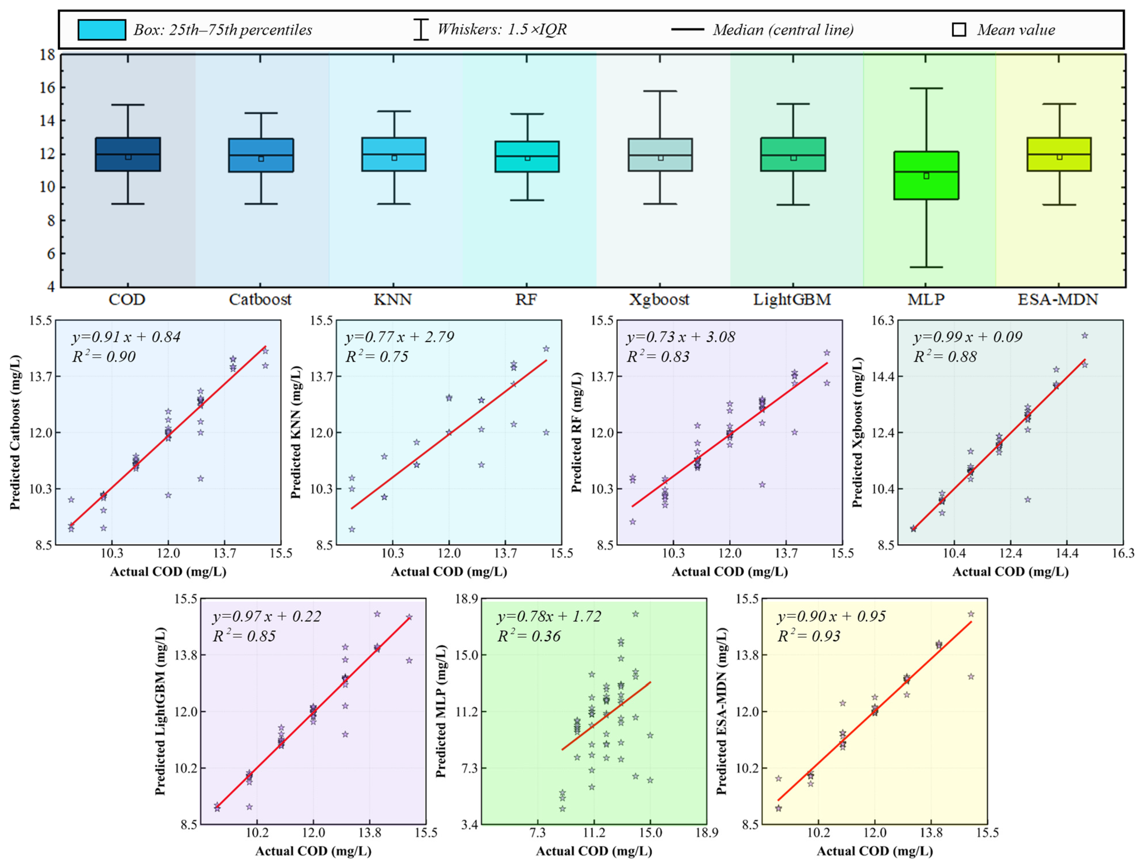
The box plot results in Figure 8 indicate that the distribution ranges of the predicted values from all models closely align with the actual COD concentrations. Among them, the predictions from CatBoost, LightGBM, and the ESA-MDN ensemble model have medians that are nearest to the true value range, with narrower interquartile ranges (IQRs) suggesting higher prediction stability. The scatter plot fitting further quantifies model accuracy, revealing that CatBoost (R² = 0.90) and ESA-MDN (R² = 0.93) demonstrate optimal linear correlations.

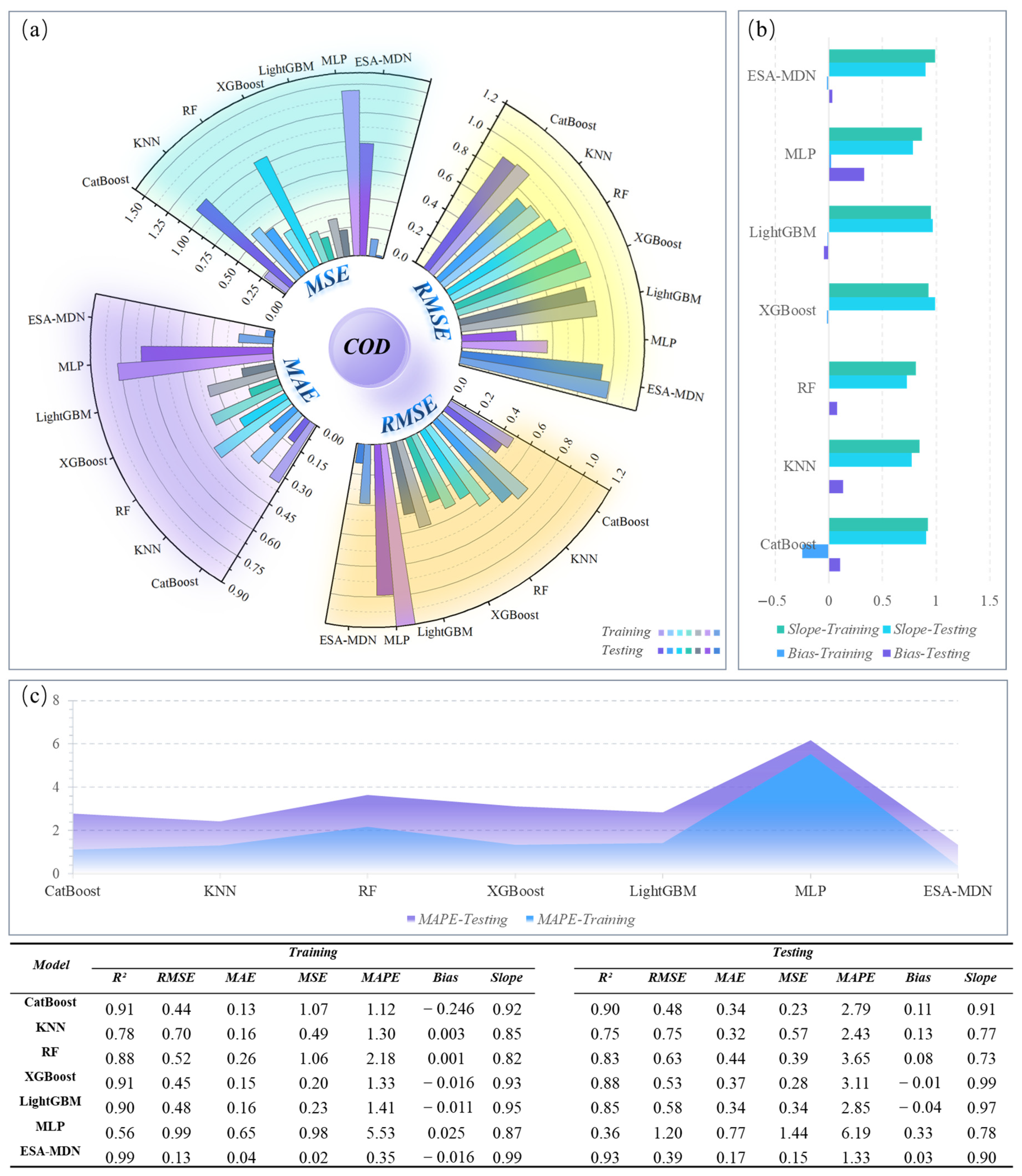
A systematic evaluation of seven models for chemical oxygen demand (COD) concentration retrieval demonstrates that ESA-MDN achieves superior performance across all metrics. The model exhibits outstanding test set results, with R² = 0.93, RMSE = 0.390, MAE = 0.17, MSE = 0.15, and MAPE = 1.33%, while maintaining near-zero bias (0.03) and near-ideal slope (0.90). The minimal performance discrepancy between training and testing phases (ΔR² = 0.06) confirms its excellent prediction accuracy and generalization capability. The comparative performance of the other models is shown in Figure 9.

3.5. TP Model Performance Analysis

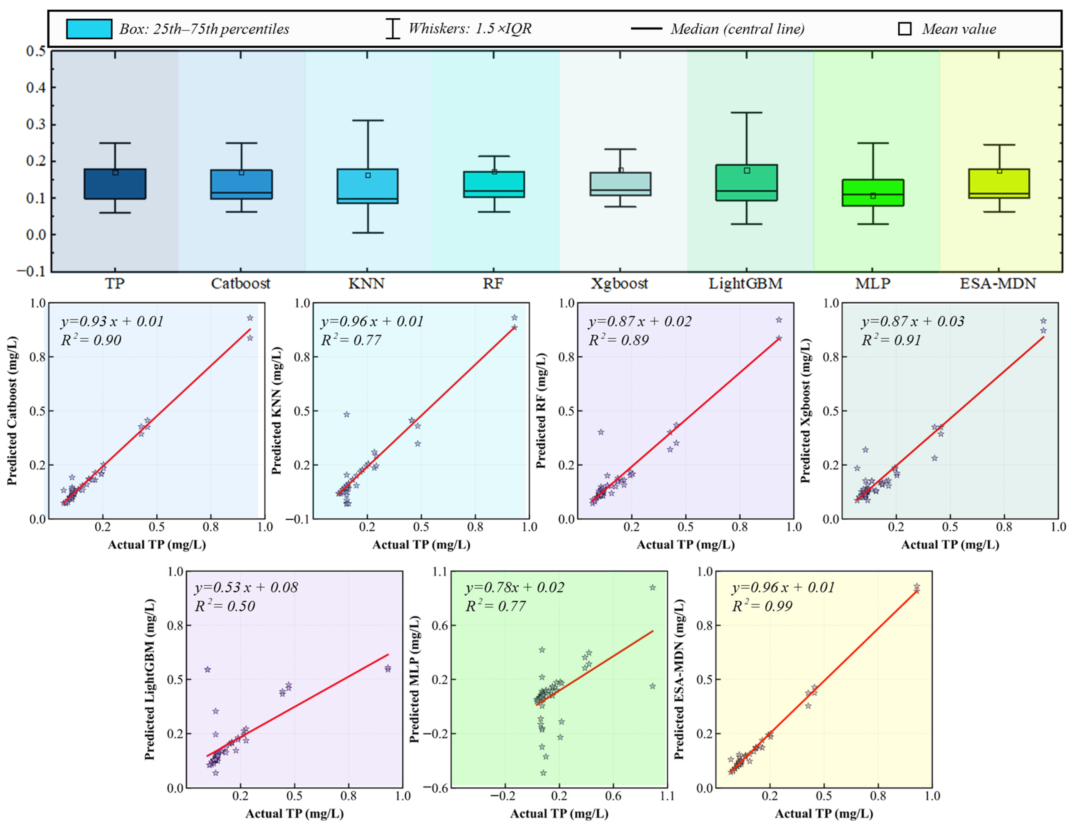
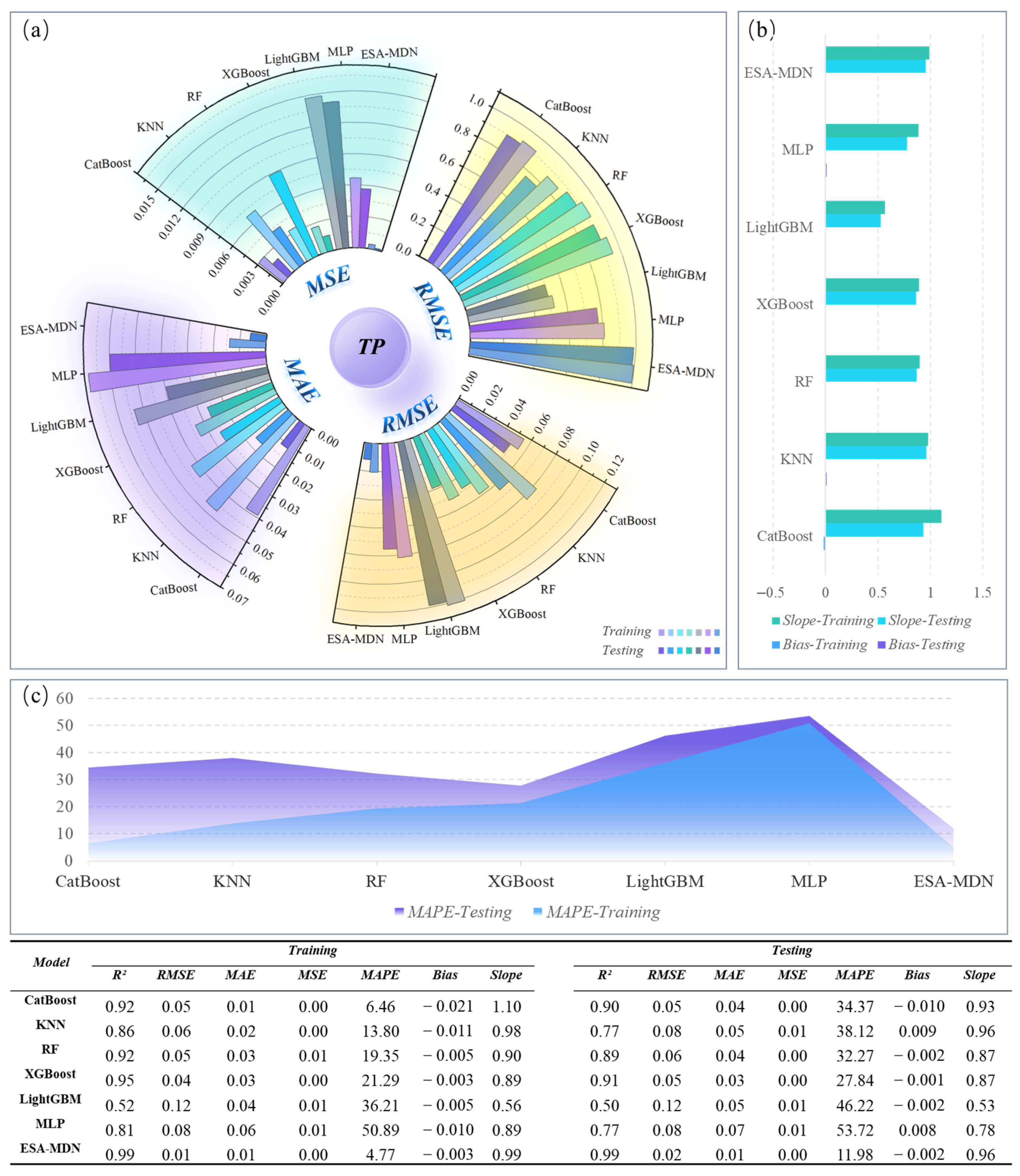
The comprehensive analysis of the box plot results reveals that KNN and LightGBM exhibit longer boxes with greater variability, whereas the boxes for CatBoost and ESA-MDN closely align with the true TP data. The scatter plot fitting results indicate that LightGBM and MLP demonstrate relatively limited predictive performance, while ESA-MDN excels in both the coefficient of determination and fitting slope, as shown in Figure 10.

Figure 11 presents the performance evaluation of seven models for total phosphorus (TP) concentration retrieval, revealing significant disparities in accuracy, error control, and generalization capability among the algorithms. The ESA-MDN model demonstrates multidimensional superiority, with test set R² = 0.99, MAE = 0.02, and slope = 0.96, exhibiting a highly concentrated error distribution (MSE = 0.0004). Comparative analysis shows that ESA-MDN achieves substantial precision enhancement in core metrics compared to other models, establishing its technical superiority for quantitative TP retrieval. By contrast, alternative models exhibit application-limiting deficiencies in specific dimensions due to inherent algorithmic constraints or parameter adaptability issues.

3.6. DO Model Performance Analysis

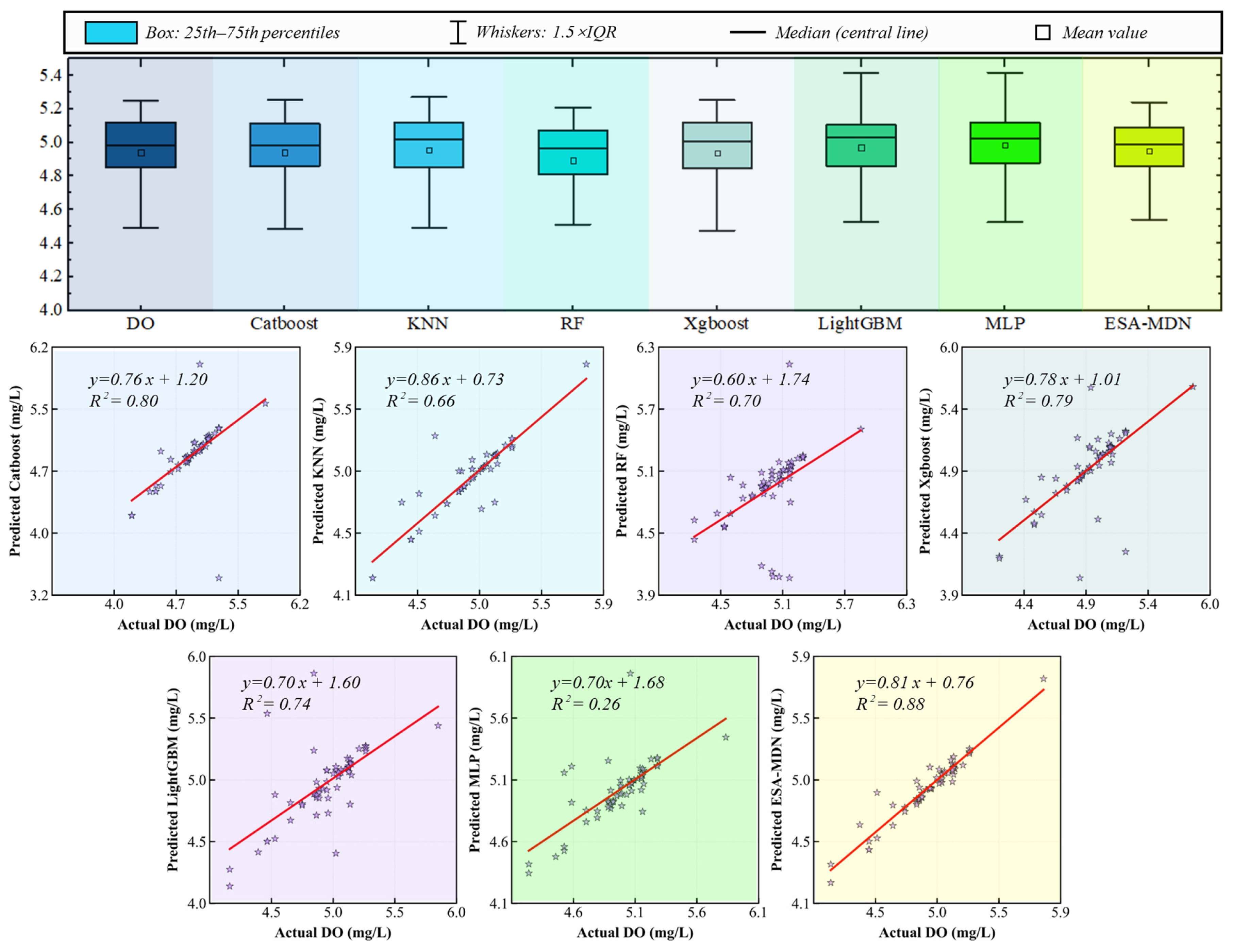
Figure 12 comprehensively presents the prediction performance for dissolved oxygen (DO) concentration based on the test set. The box plot results indicate that the predicted medians (the horizontal lines within the boxes) of all models are generally distributed around the actual values, with CatBoost and ESA-MDN showing medians that are closest to the true values, reflecting high predictive accuracy. Additionally, the scatter plot fitting analysis demonstrates that the ESA-MDN model achieves the best prediction accuracy (R² = 0.88), with a regression slope of 0.81, ranking just below KNN. However, KNN has a lower R² of 0.66, making ESA-MDN the optimal choice overall.

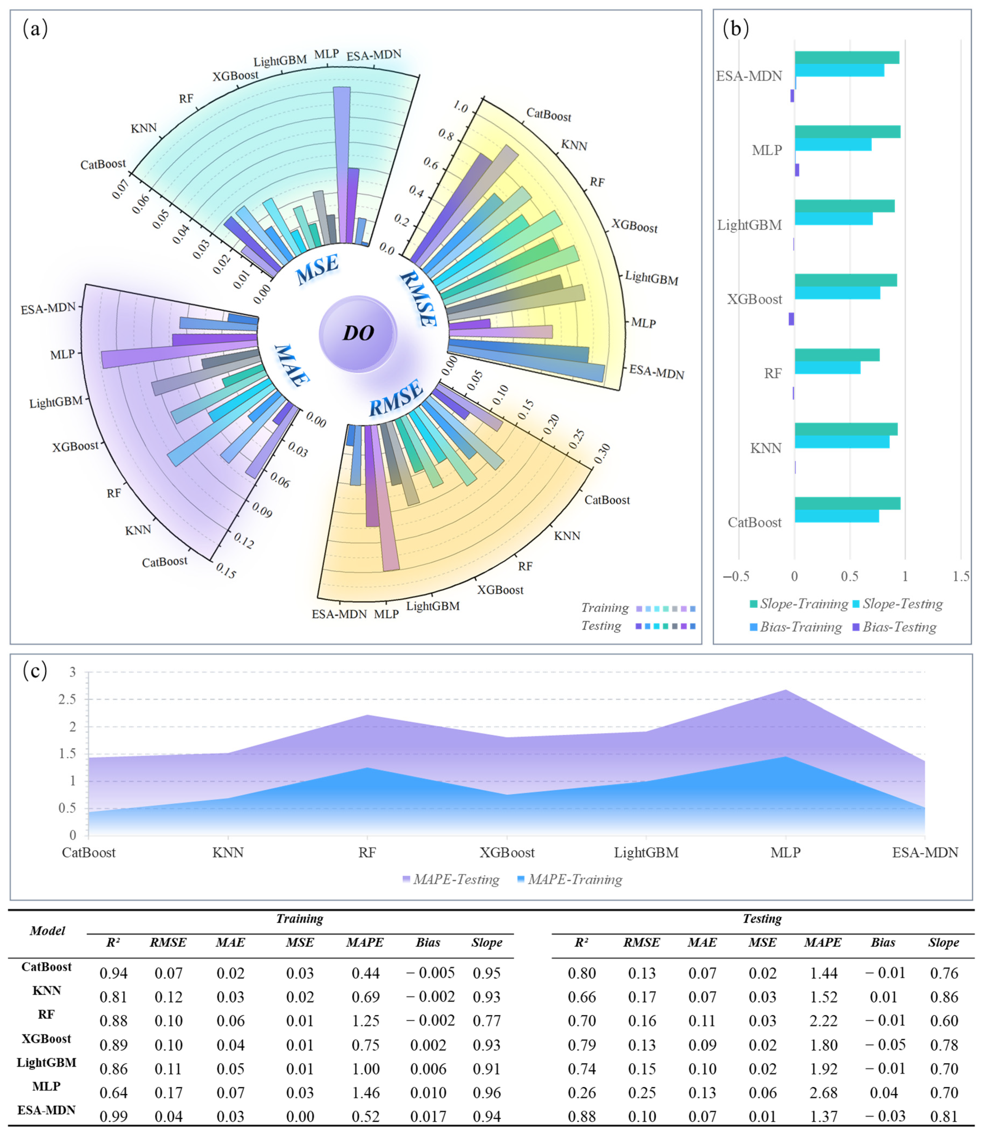
Figure 13 presents the dissolved oxygen (DO) concentration retrieval evaluation results. The findings demonstrate that the ESA-MDN model achieves optimal comprehensive performance, attaining a test set R² of 0.88 with RMSE = 0.10 and MAE = 0.07. The model exhibits the closest approximation to the ideal slope (0.81) and minimal performance discrepancy between training and testing phases (ΔR² = 0.11), confirming its suitability for aquatic DO concentration retrieval. The uniform error distribution further substantiates its superior prediction stability.

3.7. Analysis of Spatial Distribution Maps of Water Quality Parameters

The ESA-MDN model proposed in this study was employed to spatially map the concentrations of Chl-a, TSS, COD, TP, and DO in river water bodies using UAV-acquired multispectral imagery (Figure 14). Within the study area, the Chl-a concentration distribution exhibited characteristic patterns with elevated levels in tributaries and confluence zones between mainstem and tributaries, ranging primarily from 8 to 10.21 μg/L. This spatial distribution is attributed to agricultural non-point source pollution from surrounding tributary areas and direct wastewater discharge from densely populated residential zones. TSS concentrations ranged from 5.51 to 9.85 mg/L, with higher concentrations observed in the main channel, particularly in upstream village areas and downstream industrial zones where field investigations identified multiple discharge outlets potentially contributing to elevated levels. COD concentrations demonstrated a “multi-point source diffusion” pattern, with relatively higher values concentrated in downstream industrial areas. According to the GB3838-2002 standard, these measurements fell within Class I–II water quality limits (≤15 mg/L), indicating compliant but spatially variable conditions with potential pollution risks. TP concentrations spanned 0.04–0.98 mg/L, corresponding to water quality classifications ranging from Class II to V, with Class V predominantly distributed in western tributaries while the main channel exhibited Class II–IV characteristics (0.1–0.36 mg/L). DO distribution remained relatively stable throughout the study area (4.01–5.89 mg/L), meeting Class III–IV standards, with optimal oxygen levels observed in mid-to-downstream residential zones. This comprehensive spatial analysis revealed distinct pollution patterns and water quality gradients across different river segments, providing valuable insights for targeted water quality management strategies.

4. Discussion

4.1. Potential and Limitations of UAV Multispectral Imagery for Water Quality Inversion

Unmanned aerial vehicle (UAV) multispectral remote sensing, with its unique platform characteristics and sensor advantages, can effectively capture spatial pollution patterns that traditional monitoring methods often fail to identify, demonstrating irreplaceable value in urban river monitoring. Compared to in situ water sampling and hyperspectral remote sensing inversion, UAV platforms equipped with multispectral imaging systems show significant cost effectiveness and measurement precision advantages in water quality parameter inversion for urban small rivers. However, despite the effectiveness of this method in controlling monitoring costs, the limited number of spectral bands in multispectral sensors results in a generally inadequate correlation between raw reflectance data, band combination results, and ground truth measurements. This indicates a need for more refined band selection optimization based on hyperspectral data. By developing a multispectral camera tailored for water quality inversion, leveraging knowledge from hyperspectral band selection results, it was possible to significantly enhance the model’s generalization capability and robustness while maintaining cost advantages.

4.2. Advantages and Limitations of Water Quality Data Augmentation Strategies

The accuracy of water quality inversion models is closely related to the sample size, particularly in the context of machine learning and deep learning applications. However, the high costs associated with water quality sampling often limit the increase in sample size. To address this issue, this study proposes a water quality data augmentation strategy that establishes a correspondence between “multi-point sampling means and multi-pixel reflectance,” effectively overcoming the critical bottleneck of insufficient sample size in remote sensing water quality inversion. Compared to the traditional “multi-pixel mean to single-point sampling” approach, this strategy enhances the effective training sample size by an order of magnitude while maintaining sampling costs. This method leverages the spatial detail information from high-resolution UAV imagery to achieve sub-meter level accuracy in water quality-spectral matching, significantly improving the training effectiveness of machine learning models.

However, several issues remain to be addressed: (1) While this strategy increases sample data volume through spatial averaging, the relative concentration of true value points (30 sampling points corresponding to 300 pixels) reduces the spatial distribution diversity of the samples, potentially weakening the model’s ability to represent the spatial heterogeneity of water bodies. (2) Scale effects in the spectral–water quality relationship may arise when water bodies undergo dynamic changes (e.g., turbidity and flow rate), rendering the homogeneity assumption invalid. Further research is needed to enhance sample augmentation under conditions of significant water body variability. (3) Meteorological sensitivity poses challenges, particularly in conditions of cloud cover or high wind speeds, which can lead to substantial fluctuations in reflectance within the 35 cm radius. Future research will systematically integrate multidimensional environmental factors such as water turbidity, flow fields, and meteorological parameters, while also incorporating sample datasets from different regions to build a more comprehensive model analysis framework.

4.3. Applicability and Limitations of the Model in Water Quality Inversion

Ensemble learning enhances predictive performance by combining multiple models, thereby reducing the risk of overfitting and minimizing the likelihood of local optima [32,33]. Consequently, this study developed the Ensemble Self-Attention Enhanced Mixture Density Network (ESA-MDN), which integrates an ensemble learning framework with a mixture density network and incorporates a self-attention mechanism for feature enhancement. This data-driven model achieves high-precision modeling of the probability distribution of water quality parameters. Compared to traditional machine learning methods, ESA-MDN demonstrates two key advantages in water quality parameter inversion: (1) The ensemble deep learning architecture effectively captures the nonlinear relationships between water quality parameters and remote sensing features, showcasing hierarchical feature representation and strong transferability. This is particularly beneficial for non-optical active parameters, which lack obvious spectral response characteristics, where remote sensing inversion relies primarily on the indirect associations with optical active parameters or collaborative analysis of environmental factors. ESA-MDN operates as a data-driven model that significantly reduces dependence on traditional physical parameters through an end-to-end feature learning mechanism. (2) In multispectral imagery, the information from spectral channels is often limited. The self-attention mechanism establishes feature weight matrices between bands, allowing each band’s features to be dynamically adjusted based on contextual information, thereby enhancing cross-band feature interactions and deeply exploring the representational capabilities of the limited spectral channels.

Regarding model applicability, a differentiated model selection strategy should be employed based on specific requirements. When overall accuracy performance is prioritized, the ESA-MDN model outperforms others, including CatBoost, KNN, RF, XGBoost, LightGBM, and MLP, across five key metrics: R², RMSE, MAE, MAPE, and MSE. Using systematic prediction bias as a metric, the results for the Chl-a test set indicated that LightGBM (Bias = 0.01) performed best, followed by CatBoost (Bias = 0.03); for the TSS test set, RF and XGBoost showed the lowest bias (Bias = 0.02); XGBoost also excelled for the COD test set (Bias = 0.01); and for the TP test set, XGBoost had the best performance (Bias = −0.001). In terms of capturing trends in concentration changes, a slope closer to 1 accurately reflects the concentration gradient. For example, in Chl-a measurements, LightGBM had the slope closest to 1 at 0.96; for TSS and TP, both KNN and ESA-MDN achieved the highest slopes of 0.86 and 0.96, respectively; XGBoost had the highest slope for COD (Slope = 0.99); and KNN showed the highest slope for DO (Slope = 0.86). These findings provide important guidance for selecting water quality remote sensing models, suggesting that ESA-MDN should be chosen as the inversion model in accuracy-focused applications. Conversely, in bias-sensitive applications or scenarios requiring high-precision trend analysis, targeted analyses and selections should be conducted based on the specifics of experimental data.

Considering that the current model is entirely data-driven, future research should integrate optical physical models of water bodies by constructing a hybrid modeling framework that combines “physical mechanism constraints and data-driven approaches.” This integration aims to enhance the model’s generalization capabilities and physical interpretability in complex optical environments. Additionally, experiments should be conducted in water bodies across different environments to further quantify the variations in uncertainty across parameters and regions, as well as to explore how spatiotemporal distribution maps can be effectively utilized for water pollution management. It is also essential to strengthen interdisciplinary collaboration, organically merging the latest advancements in remote sensing technology, hydrology, ecology, and artificial intelligence to collectively promote innovative developments in water quality remote sensing monitoring technologies.

5. Conclusions

The water quality status of urban rivers results from the combined effects of water body characteristics, anthropogenic disturbances along riverbanks, and natural environmental factors. This multifactorial coupling leads to pronounced spatial heterogeneity and temporal dynamics in water quality parameters. Remote sensing technology, with its outstanding advantages in spatiotemporal dynamic monitoring, can effectively compensate for the limitations of conventional water quality monitoring methods. However, constrained by insufficient water quality samples and structural deficiencies in existing models, current water quality retrieval models generally exhibit inadequate prediction accuracy and generalization performance in complex urban river network environments. To address this issue, our study proposes a water quality data enhancement method at the data level. Taking the sampling point as the central pixel, we established a 35 cm buffer zone to extract image reflectance data from both this central pixel and nine randomly selected pixels within the buffer. These data were then matched with laboratory analysis results of composite water samples (3 L) collected within a 35 cm radius of corresponding sampling points, thereby achieving data volume expansion. This approach significantly improved the spatial representativeness of sample information and enhanced data utilization efficiency. At the model level, we developed the ESA-MDN model, which integrates ensemble learning strategies with deep learning approaches to perform the retrieval of five water quality parameters: Chl-a (R² = 0.98, RMSE = 0.31), TSS (R² = 0.93, RMSE = 0.27), COD (R² = 0.93, RMSE = 0.39), TP (R² = 0.99, RMSE = 0.02), and DO (R² = 0.88, RMSE = 0.1). This study provides a novel modeling framework for water quality retrieval in complex urban river networks. Future research should focus on collecting additional ground-based water quality measurements and UAV multispectral data across various water body types and seasonal conditions to further validate the model’s generalization capabilities under different environmental scenarios.

References

1. Hermes, A.L.; Logan, M.N.; Poulin, B.A.; McKenna, A.M.; Dawson, T.E.; Borch, T.; Hinckley, E.-L.S. Agricultural Sulfur Applications Alter the Quantity and Composition of Dissolved Organic Matter from Field-to-Watershed Scales. Environ. Sci. Technol. 2023, 57, 10019–10029. [Google Scholar] [CrossRef] [PubMed]
2. Stets, E.G.; Sprague, L.A.; Oelsner, G.P.; Johnson, H.M.; Murphy, J.C.; Ryberg, K.; Vecchia, A.V.; Zuellig, R.E.; Falcone, J.A.; Riskin, M.L. Landscape Drivers of Dynamic Change in Water Quality of U.S. Rivers. Environ. Sci. Technol. 2020, 54, 4336–4343. [Google Scholar] [CrossRef] [PubMed]
3. Roy, S.; Bose, A.; Basak, D.; Chowdhury, I.R. Towards Sustainable Society: The Sustainable Livelihood Security (SLS) Approach for Prioritizing Development and Understanding Sustainability: An Insight from West Bengal, India. Environ. Dev. Sustain. 2023, 26, 20095–20126. [Google Scholar] [CrossRef]
4. Zhou, X.; Liu, C.; Carrion, D.; Akbar, A.; Wang, H. Spectro-Environmental Factors Integrated Ensemble Learning for Urban River Network Water Quality Remote Sensing. Water Res. 2024, 267, 122544. [Google Scholar] [CrossRef] [PubMed]
5. Rahat, S.H.; Steissberg, T.; Chang, W.; Chen, X.; Mandavya, G.; Tracy, J.; Wasti, A.; Atreya, G.; Saki, S.; Bhuiyan, M.A.E. Remote Sensing-Enabled Machine Learning for River Water Quality Modeling under Multidimensional Uncertainty. Sci. Total Environ. 2023, 898, 165504. [Google Scholar] [CrossRef]
6. Wang, H.; Liu, C.; Li, L.; Kong, Y.; Akbar, A.; Zhou, X. High-Precision Inversion of Urban River Water Quality via Integration of Riparian Spatial Structures and River Spectral Signatures. Water Res. 2025, 278, 123378. [Google Scholar] [CrossRef]
7. Lu, Q.; Si, W.; Wei, L.; Li, Z.; Xia, Z.; Ye, S.; Xia, Y. Retrieval of Water Quality from UAV-Borne Hyperspectral Imagery: A Comparative Study of Machine Learning Algorithms. Remote Sens. 2021, 13, 3928. [Google Scholar] [CrossRef]
8. Jiang, Q.; Xu, L.; Sun, S.; Wang, M.; Xiao, H. Retrieval Model for Total Nitrogen Concentration Based on UAV Hyper Spectral Remote Sensing Data and Machine Learning Algorithms—A Case Study in the Miyun Reservoir, China. Ecol. Indic. 2021, 124, 107356. [Google Scholar]
9. Giles, A.B.; Correa, R.E.; Santos, I.R.; Kelaher, B. Using Multispectral Drones to Predict Water Quality in a Subtropical Estuary. Environ. Technol. 2024, 45, 1300–1312. [Google Scholar] [CrossRef]
10. Niroumand-Jadidi, M.; Bovolo, F.; Bruzzone, L. Novel Spectra-Derived Features for Empirical Retrieval of Water Quality Parameters: Demonstrations for OLI, MSI, and OLCI Sensors. IEEE Trans. Geosci. Remote Sens. 2019, 57, 10285–10300. [Google Scholar] [CrossRef]
11. Harringmeyer, J.P.; Ghosh, N.; Weiser, M.W.; Thompson, D.R.; Simard, M.; Lohrenz, S.E.; Fichot, C.G. A Hyperspectral View of the Nearshore Mississippi River Delta: Characterizing Suspended Particles in Coastal Wetlands Using Imaging Spectroscopy. Remote Sens. Environ. 2024, 301, 113943. [Google Scholar] [CrossRef]
12. Li, J.; Wang, G.; Sun, S.; Ma, J.; Guo, L.; Song, C.; Lin, S. Mapping and Reconstruct Suspended Sediment Dynamics (1986–2021) in the Source Region of the Yangtze River, Qinghai-Tibet Plateau Using Google Earth Engine. Remote Sens. Environ. 2025, 317, 114533. [Google Scholar] [CrossRef]
13. Sun, Y.; Wang, D.; Li, L.; Ning, R.; Yu, S.; Gao, N. Application of Remote Sensing Technology in Water Quality Monitoring: From Traditional Approaches to Artificial Intelligence. Water Res. 2024, 267, 122546. [Google Scholar] [CrossRef] [PubMed]
14. Binding, C.E.; Pizzolato, L.; Zeng, C. EOLakeWatch; Delivering a Comprehensive Suite of Remote Sensing Algal Bloom Indices for Enhanced Monitoring of Canadian Eutrophic Lakes. Ecol. Indic. 2021, 121, 106999. [Google Scholar] [CrossRef]
15. Ji, C.; Zhang, Y.; Nejstgaard, J.C.; Ogashawara, I. Assessment of the Sediment Load in the Pearl River Estuary Based on Land Use and Land Cover Changes. CATENA 2025, 250, 108726. [Google Scholar] [CrossRef]
16. Moon, J.; Jung, S.; Suh, S.; Pyo, J. Development of Deep Learning Quantization Framework for Remote Sensing Edge Device to Estimate Inland Water Quality in South Korea. Water Res. 2025, 283, 123760. [Google Scholar] [CrossRef]
17. Sagan, V.; Peterson, K.T.; Maimaitijiang, M.; Sidike, P.; Sloan, J.; Greeling, B.A.; Maalouf, S.; Adams, C. Monitoring Inland Water Quality Using Remote Sensing: Potential and Limitations of Spectral Indices, Bio-Optical Simulations, Machine Learning, and Cloud Computing. Earth-Sci. Rev. 2020, 205, 103187. [Google Scholar] [CrossRef]
18. Tesfaye, A. Remote Sensing-Based Water Quality Parameters Retrieval Methods: A Review. East Afr. J. Environ. Nat. Resour. 2024, 7, 80–97. [Google Scholar] [CrossRef]
19. Cai, X.; Li, Y.; Lei, S.; Zeng, S.; Zhao, Z.; Lyu, H.; Dong, X.; Li, J.; Wang, H.; Xu, J. A Hybrid Remote Sensing Approach for Estimating Chemical Oxygen Demand Concentration in Optically Complex Waters: A Case Study in Inland Lake Waters in Eastern China. Sci. Total Environ. 2023, 856, 158869. [Google Scholar] [CrossRef]
20. Chen, S.; Han, L.; Chen, X.; Li, D.; Sun, L.; Li, Y. Estimating Wide Range Total Suspended Solids Concentrations from MODIS 250-m Imageries: An Improved Method. ISPRS J. Photogramm. Remote Sens. 2015, 99, 58–69. [Google Scholar] [CrossRef]
21. Ngoc, D.D.; Loisel, H.; Jamet, C.; Vantrepotte, V.; Duforêt-Gaurier, L.; Minh, C.D.; Mangin, A. Coastal and Inland Water Pixels Extraction Algorithm (WiPE) from Spectral Shape Analysis and HSV Transformation Applied to Landsat 8 OLI and Sentinel-2 MSI. Remote Sens. Environ. 2019, 223, 208–228. [Google Scholar] [CrossRef]
22. Zhu, X.X.; Tuia, D.; Mou, L.; Xia, G.-S.; Zhang, L.; Xu, F.; Fraundorfer, F. Deep Learning in Remote Sensing: A Comprehensive Review and List of Resources. IEEE Geosci. Remote Sens. Mag. 2017, 5, 8–36. [Google Scholar] [CrossRef]
23. Li, X.; Yang, Y.; Ishizaka, J.; Li, X. Global Estimation of Phytoplankton Pigment Concentrations from Satellite Data Using a Deep-Learning-Based Model. Remote Sens. Environ. 2023, 294, 113628. [Google Scholar] [CrossRef]
24. Zhang, D.; Shi, K.; Wang, W.; Wang, X.; Zhang, Y.; Qin, B.; Zhu, M.; Dong, B.; Zhang, Y. An Optical Mechanism-Based Deep Learning Approach for Deriving Water Trophic State of China’s Lakes from Landsat Images. Water Res. 2024, 252, 121181. [Google Scholar] [CrossRef]
25. Guo, H.; Huang, J.J.; Zhu, X.; Tian, S.; Wang, B. Spatiotemporal Variation Reconstruction of Total Phosphorus in the Great Lakes since 2002 Using Remote Sensing and Deep Neural Network. Water Res. 2024, 255, 121493. [Google Scholar] [CrossRef] [PubMed]
26. Xiong, J.; Lin, C.; Cao, Z.; Hu, M.; Xue, K.; Chen, X.; Ma, R. Development of Remote Sensing Algorithm for Total Phosphorus Concentration in Eutrophic Lakes: Conventional or Machine Learning? Water Res. 2022, 215, 118213. [Google Scholar] [CrossRef] [PubMed]
27. Gan, M.; Lai, X.; Guo, Y.; Chen, Y.; Pan, S.; Zhang, Y. Floodplain Lake Water Level Prediction with Strong River-Lake Interaction Using the Ensemble Learning LightGBM. Water Resour. Manag. 2024, 38, 5305–5321. [Google Scholar] [CrossRef]
28. Mienye, I.D.; Sun, Y. A Survey of Ensemble Learning: Concepts, Algorithms, Applications, and Prospects. IEEE Access 2022, 10, 99129–99149. [Google Scholar] [CrossRef]
29. Ehteram, M.; Ahmed, A.N.; Sherif, M.; El-Shafie, A. An Advanced Deep Learning Model for Predicting Water Quality Index. Ecol. Indic. 2024, 160, 111806. [Google Scholar] [CrossRef]
30. Tripathy, K.P.; Mishra, A.K. Deep Learning in Hydrology and Water Resources Disciplines: Concepts, Methods, Applications, and Research Directions. J. Hydrol. 2024, 628, 130458. [Google Scholar]
31. GB 3838-2002; Environmental Quality Standards for Surface Water. Ministry of Ecology and Environment of the People’s Republic of China: Beijing, China, 2002.
32. Mohseni, U.; Pande, C.B.; Pal, S.C.; Alshehri, F. Prediction of Weighted Arithmetic Water Quality Index for Urban Water Quality Using Ensemble Machine Learning Model. Chemosphere 2024, 352, 141393. [Google Scholar] [CrossRef]
33. Satish, N.; Anmala, J.; Rajitha, K.; Varma, M.R. A Stacking ANN Ensemble Model of ML Models for Stream Water Quality Prediction of Godavari River Basin, India. Ecol. Inform. 2024, 80, 102500. [Google Scholar] [CrossRef]
Figure 1. Geographic location schematic diagram of the study area and distribution of sampling sites: (a) location schematic diagram of the study area; (b) geographic location of Shanghai; and (c) distribution map of UAV aerial survey results and sampling points.
Remotesensing 17 03202 g001
Figure 2. Schematic diagram of random pixel extraction within UAV image buffer zone.
Remotesensing 17 03202 g002
Figure 3. Ensemble Self-Attention Enhanced Mixture Density Network.
Remotesensing 17 03202 g003
Figure 4. Box plot of the numerical distribution of Chl-a test set inversion results and scatter plot with linear fitting.
Remotesensing 17 03202 g004
Figure 5. Performance evaluation of Chl-a inversion model: (a) accuracy metrics (R2, RMSE, MAE, and MSE); (b) bias and consistency; and (c) MAPE assessment.
Remotesensing 17 03202 g005
Figure 6. Box plot of the numerical distribution of TSS test set inversion results and scatter plot with linear fitting.
Remotesensing 17 03202 g006
Figure 7. Performance evaluation of TSS inversion model: (a) accuracy metrics (R2, RMSE, MAE, and MSE); (b) bias and consistency; and (c) MAPE assessment.
Remotesensing 17 03202 g007
Figure 8. Box plot of the numerical distribution of COD test set inversion results and scatter plot with linear fitting.
Remotesensing 17 03202 g008
Figure 9. Performance evaluation of COD inversion model: (a) accuracy metrics (R2, RMSE, MAE, and MSE); (b) bias and consistency; and (c) MAPE assessment.
Remotesensing 17 03202 g009
Figure 10. Box plot of the numerical distribution of TP test set inversion results and scatter plot with linear fitting.
Remotesensing 17 03202 g010
Figure 11. Performance evaluation of TP inversion model: (a) accuracy metrics (R2, RMSE, MAE, and MSE); (b) bias and consistency; and (c) MAPE assessment.
Remotesensing 17 03202 g011
Figure 12. Box plot of the numerical distribution of DO test set inversion results and scatter plot with linear fitting.
Remotesensing 17 03202 g012
Figure 13. Performance evaluation of DO inversion model: (a) accuracy metrics (R2, RMSE, MAE, and MSE); (b) bias and consistency; and (c) MAPE assessment.
Remotesensing 17 03202 g013
Figure 14. UAV-borne remote sensing water quality inversion results: (a) spatial distribution of Chl-a concentration; (b) spatial distribution of SS concentration; (c) spatial distribution of COD concentration; (d) spatial distribution of TP concentration; and (e) spatial distribution of DO concentration.
Remotesensing 17 03202 g014