Article

Oil Spill Identification with Marine Radar Using Feature Augmentation and Improved Firefly Optimization Algorithm

1
Shenzhen Institute of Guangdong Ocean University, Shenzhen 518116, China
2
Naval Architecture and Shipping College, Guangdong Ocean University, Zhanjiang 524091, China
3
Technical Research Center for Ship Intelligence and Safety Engineering of Guangdong Province, Zhanjiang 524088, China
4
Guangdong Provincial Key Laboratory of Intelligent Equipment for South China Sea Marine Ranching, Guangdong Ocean University, Zhanjiang 524088, China
5
Navigation College, Dalian Maritime University, Dalian 116026, China
*
Author to whom correspondence should be addressed.
Remote Sens. 2025, 17(18), 3148; https://doi.org/10.3390/rs17183148
Submission received: 23 July 2025 / Revised: 7 September 2025 / Accepted: 9 September 2025 / Published: 10 September 2025

Abstract

Highlights

What are the main findings?
  • To address the need for precise extraction of oil spill regions of interest, a Local Binary Pattern (LBP) feature enhancement method was introduced.
  • Specific optimizations were strategically applied to the Firefly Optimization Algorithm for better adapt to the complex noise characteristics of marine radar signals. These targeted improvements enabled the algorithm to more effectively distinguish oil film targets from background interference.
What is the implication of the main finding?
  • Precise identification of regions of interest (ROIs) serves as the foundational step in oil spill monitoring systems. The extracted ROIs thus provide the critical spatial context for achieving high-confidence oil film detection through feature fusion enhancement method.
  • The improved firefly algorithm demonstrates superior adaptability for oil film segmentation tasks in complex marine radar imagery, effectively addressing challenges posed by sea clutter and low contrast. This innovation provides a robust technical framework for real-time marine oil spill monitoring systems, enabling high-confidence detection in dynamic ocean environments.

Abstract

Oil spill accidents pose a grave threat to marine ecosystems, human economy, and public health. Consequently, expeditious and efficacious oil spill detection technology is imperative for the pollution mitigation and the health preservation in the marine environment. This study proposed a marine radar oil spill detection method based on Local Binary Patterns (LBP), Histogram of Oriented Gradient (HOG), and an improved Firefly Optimization Algorithm (IFA). In the stage of image pre-processing, the oil film features were significantly enhanced through three steps. The LBP features were extracted from the preprocessed image. Then, the mean filtering was used to smooth out the LBP features. Subsequently, the HOG statistical features were extracted from the filtered LBP feature map. After the feature enhancement, the oil spill regions were accurately extracted by using K-Means clustering algorithm. Next, an IFA model was used to classify oil films. Compared with traditional Firefly Optimization Algorithm (FA) algorithm, the IFA method is suitable for oil film segmentation tasks in marine radar data. The proposed method can achieve accuracy segmentation and provide a new technical path for marine oil spill monitoring.

1. Introduction

With the swift economic progression witnessed globally, the worldwide demand for crude oil is on a steady rise [1]. Presently, maritime transportation is the predominant mode for oil delivery due to its low cost-effectiveness, consequently elevating the likelihood of marine oil spill incidents. The escalating frequency of marine oil spill catastrophes has inflicted severe damage upon the ocean ecosystem [2]. Simultaneously, these oil leakages constitute a significant peril to human economic endeavors [3]. On 25 July 2020 the Japanese cargo vessel Wakashio was grounded in the southeastern waters off Mauritius, an island nation located in the Indian Ocean. A minimum of 1000 tons of fuel was spilled, resulting in severe contamination of the internationally significant wetlands and marine protected regions in southeast Mauritius [4]. On 20 April 2010, the Deepwater Horizon drilling rig experienced a blowout followed by an explosion. This accident led to 11 fatalities and 17 injuries. The underwater oil well persisted in leaking crude oil for 87 consecutive days, with the total spillage reaching approximately 3.19 million barrels [5]. The oil slicks inflicted severe destruction on coral reefs, mangrove forests, and fish habitats, placing certain species in peril of extinction [6]. The oil films are formed on the sea surface, resulting in hypoxic conditions in the marine environment [7]. Due to this oxygen deficiency, plankton, fish, and shrimp perish in large quantities, undermining the foundation of the marine food chain [8]. Toxic substances, including benzene derivatives and heavy metals, are progressively concentrated through the food chain, inflicting lethal harm on apex predators and humans [9]. Polycyclic aromatic hydrocarbons present in petroleum exhibit carcinogenic, teratogenic, and mutagenic properties, capable of damaging the DNA structure of marine organisms and impairing their reproductive capacity [10].
Currently, the predominant international approaches for monitoring oil spills encompass satellite remote sensing, aerial surveillance, vessel-based observation, and buoy deployed detection [11,12]. Fan et al. [13] introduced a multi-feature semantic complementation network (MFSCNet) within a unified framework. This network was specifically designed for the localization and segmentation of oil spills in SAR images. The detection accuracy of the positioning frame can be significantly improved. Chen et al. [14] proposed a hyperspectral ocean oil spill image segmentation model with multi-scale feature fusion (MFFHOSS-Net). This innovative model effectively boosted the precision in segmenting oil spill regions. Yang et al. [15] put forward a model based on the graph convolutional architecture and spatial-spectral information fusion. This model demonstrated outstanding performance in the oil spills detection. Ren et al. [16] introduced a deep-learning-based approach to correcting numerically forecasted sea surface dynamic fields. This method can accurately predict the development of the oil spill disaster. Akhmedov et al. [17] utilized the YOLOv8 segmentation network to train an oil spill detection model for accurately identifying oil spills. The outcomes revealed that real-time oil spill detection can be efficiently achieved. Prajapati et al. [18] proposed a GSCAT-UNET model for oil spill discrimination from lookalikes. The segmentation accuracy and robustness were markedly enhanced by their model. Furthermore, the problems posed by SAR data complexity and dataset imbalance are effectively addressed.
Traditional oil spill detection technologies exhibit some limitations. Visible light technology, for instance, depends on natural illumination and is rendered ineffective at night or under severe weather conditions. Marine radar exhibits distinct advantages in the detection of oil spills, primarily manifested in its capability to operate under all weather conditions in all-day, as well as its sensitivity to alterations in the surface roughness of oil films [19]. The application of marine radar technology of oil spill monitoring enables timely identification of such spills, swift response post-disaster, and more effective mitigation of marine pollution [20].
In this study, a novel method based on an improved Firefly Optimization Algorithm (IFA) for detecting marine oil spills is proposed. Initially, the original radar images containing oil spills are preprocessed. Subsequently, LBP features are extracted from the preprocessed images and further smoothed by using mean filtering. Then, HOG features are computed from the smoothed Local Binary Pattern (LBP) feature map. Next, the K-Means clustering algorithm is applied to classify the Regions of Interest (ROIs). Afterwards, an IFA model is employed to segment the oils roughly. Finally, the detection results were finely screened out. The IFA model is tailored for the oil film segmentation task within marine radar data. The convergence speed and global search capability of the traditional algorithm are markedly enhanced by the IFA, which incorporates strategies like adaptive step size, a multi-group cooperation mechanism, and the Lagrange multiplier. Premature convergence issues are effectively circumvented through its implementation. For instance, the adaptive step size is capable of being dynamically modified in line with the aggregation level of fireflies. This modification helps prevent initial oscillation and subsequent stagnation. Parallel searches by multiple groups of fireflies broaden the spatial coverage. The Lagrange multiplier method can effectively handle intricate constraints. These enhancements enable the algorithm to demonstrate superior accuracy and stability in multi-threshold segmentation scenarios. The research objective is to accurately identify offshore oil film targets, construct a real-time monitoring system, and provide efficient decision-making support for emergency oil spill cleanup.
The structure of this paper is as follows: Section 2 meticulously delineates the data employed in this research along with the methodologies adopted. Section 3 then proceeds to present the experimental results in a clear and comprehensive manner. In Section 4, the proposed method is compared with other methods. Section 5 provides a detailed and systematic summarization of the entire study.

2. Experimental Data and Methods

2.1. Experimental Data

The experimental data was gathered from the teaching internship Yukun, operated by Dalian Maritime University, during the cruise, as shown in Figure 1. The collection platform employed X-band marine radar for near real-time surveillance. The marine radar system utilized Antennas to transmit microwave signals with precise wavelengths for targeting sea zones. Upon encountering diverse oceanic targets such as oil films, waves, islands, and other obstructions, these microwave signals were reflected from the sea surface. The existence of an oil slick on the sea surface notably influences the reflection orientation of microwave signals. It diminished the surface tension of the seawater, rendering the surface more even. This smoothness subsequently decreased the Bragg scattering of the reflected electromagnetic waves, effectively dampening the echo signals. Consequently, on radar imagery, the surface covered by the oil slick manifested as a comparatively dim region owing to the weakened echo signals. In contrast, the perimeters of the oil slick exhibited a relatively bright appearance, generating a stark contrast that facilitates detection. The radar data featured an image dimension of 1024 × 1024 pixels, as shown in Figure 2. The effective detection scope of the radar data spaned 0.75 nautical miles. The parameters of the marine radar equipment are shown in Table 1.

2.2. Pre-Processing Data

The initial radar images were subjected to pre-processing through five crucial procedures—coordinate system conversion, co-frequency interference reduction, spot inhibition, global grayscale correction, and local contrast enhancement—as depicted in Figure 3. These steps were implemented with the aim of minimizing noise disruption and simultaneously enhancing the discernibility of oil film features.

2.2.1. Coordinate System Conversion

Marine radar usually applies data in Polar coordinates for intuitive navigation operations. For ease of oil film segmentation, the original data was transformed into a Cartesian coordinate framework, with angles designated as the horizontal axis and distances as the vertical axis, as shown in Figure 4.

2.2.2. Co-Frequency Interference Noise Reduction

Radar images were subjected to co-frequency interference, which denoted the noise produced by adjacent radars or other electromagnetic apparatuses by utilizing identical or analogous frequency ranges. This interference manifested as periodic streaks or striped noise, typically presenting as horizontal or diagonal, regularly patterned bright and dark streaks within the image. Such interference led to a degradation in image quality and hampered oil film detection [21]. The noise edges were sharpened through the Laplacian operator. Subsequently, the interference-affected region was isolated by using Otsu threshold segmentation. The contaminated pixels were substituted with the average value of adjacent non-noise pixels along the horizontal axis [22,23]. This approach effectively suppressed interference while maintaining the continuity of the background radar echo, as shown in Figure 5.

2.2.3. Spot Inhibition

The speckle noise in radar images was identified as multiplicative noise, which arose from the stochastic interference of coherent waves. It was manifested as granular, randomly distributed bright and dark patches on the image. This noise significantly degrades the signal-to-noise ratio and impairs the visual quality of the image [24]. Speckle noise in radar images was screened in the pre-processing by using a dual-threshold method. Through median filtering, a marked enhancement in the uniformity and target discernibility of radar images was attained, as shown in Figure 6.

2.2.4. Global Grayscale Correction

The global grayscale correction was applied to radar images for addressing the issue of inconsistent overall brightness distribution [25]. A grayscale correction matrix [26] was employed here to globally map and modify the pixel values of the image. The purpose was to remove the local brightness distortion that stemmed from factors such as inconsistent radar system gain, distance-related attenuation, or environmental interference, as shown in Figure 7.

2.2.5. Local Contrast Enhancement

The objective of local contrast enhancement was to elevate the discernibility of detailed information within the image. The Contrast Constrained Adaptive Histogram Equalization (CLAHE) model was used here to automatically adjust local brightness. The visibility of details in dim or low-contrast zones was effectively upgraded [27], as shown in Figure 8.

2.3. Local Binary Pattern

LBP is a classical operator for image local texture feature extraction. It demonstrates robustness towards illumination alterations [28]. Rotation invariance is also a feature that it possesses. The calculation process of LBP feature value is shown in Figure 9.
The traditional extraction process of LBP features is as follows:
(1)
LBP eigenvalues are extracted from the given image as:
L B P P , R x c , y c = p = 0 P 1   s ( g p g c ) · 2 p  
where L B P P , R x c , y c is a LBP eigenvalue in the local window, x c , y c is the coordinate of the current central pixel in the local window, P is the total number of neighborhood pixels, R is neighborhood radius, g c is the gray value of the center pixel x c , y c , g p is the gray value of the p-th neighborhood pixel, s ( g p g c ) is a symbolic function.
(2)
Then, a mean filtering of the 64 × 64 window was performed on the LBP feature map.

2.4. Histogram of Oriented Gradient

The Histogram of oriented gradient (HOG) is a widely used feature descriptor for object detection in the field of computer vision and image processing. The construction approach involves the computation and enumeration of the gradient orientation within local image regions [29]. The filtered LBP feature map was used here for extracting HOG features. The specific extraction process includes the following four steps:
(1)
Gradient calculation
The horizontal gradient G x and the vertical gradient G y were used to convolve with the image I:
G x = I   × 1   0   1 , G y = I   × 1 0 1
Then, the gradient amplitude M ( x , y ) is:
M x , y = G x 2 + G y 2 , θ ( x , y ) = a r c t a n ( G y G x ) [ 0 , π )
where θ ( x , y ) is the direction.
(2)
Cell histogram statistics
The sum of the gradient amplitudes h b of the bth bin interval in the histogram is:
h b = x , y c e l l   M ( x , y ) · δ [ θ x , y b i n b ]
where b i n b is the direction interval corresponding to the bth bin in the histogram, and δ [ θ x , y b i n b ] is the indicator function.
(3)
Block normalization
The adjacent 2 × 2 cell units were combined into blocks, and the histogram vector h in the block was normalized:
h n o r m = h h 2 2 + ϵ 2 , ϵ = 10 4
where h n o r m is the normalized histogram vector, h is the original histogram vector, and ϵ is the smoothing factor used to avoid dividing by zero.
(4)
Feature stitching
The normalized histograms of all blocks are concatenated to obtain the final HOG feature vector f H O G :
f H O G = [ h n o r m 1 , h n o r m 2 , ]
where h n o r m i is the i-th normalized local histogram block vector.

2.5. K-Means Clustering Algorithm

K-means represents a classic unsupervised learning algorithm. It is applied to partition an unlabeled dataset into K distinct clusters. The data points within an identical cluster are rendered as similar as feasible, while those in separate clusters are made as dissimilar as possible. It is one of the most commonly used clustering algorithms in the field of data mining and pattern recognition [30]. The specific classification process includes initialization, allocating data points to clusters, updating centroids, repeating iteration and outputting clustering results.
(1)
Initializing centroids
Randomly select K data points as the initial centroids { μ 1 , μ 2 , , μ K } .
(2)
Allocating data points to K clusters
Calculate the distance from each data point xi to all centroids:
d ( x i , μ k ) = x i μ k 2
where d ( x i , μ k ) is the distance from the data point xi to the centroid μk. x i μ k is the difference vector between the data point and the centroid. Then, xi is assigned to the cluster corresponding to the nearest difference:
S k = { x i a r g   m i n d k ( x i , μ k ) }
where Sk is the data point set of the kth cluster.
(3)
Updating centroids
Recalculate the centroid of each cluster μ k according to the current cluster allocation:
μ k = 1 | S k | x i S k   x i
(4)
Repeating iteration
Execute steps (2) and (3) alternately until the termination conditions are met.
(5)
Outputting clustering results
Finally, K clusters { S 1 , S 2 , , S K } and their centroids { μ 1 , μ 2 , , μ K } are obtained.

2.6. The Improved Firefly Optimization Algorithm

The Firefly Optimization Algorithm (FA) represents a swarm intelligence-based optimization approach. It draws inspiration from the natural luminescent behavior exhibited by fireflies. Specifically, it is modeled after the flickering phenomenon where fireflies emit light signals to allure potential mates or capture prey. The fundamental concept is that fireflies with lower brightness are drawn towards those with higher brightness. This brightness level is directly linked to the objective function value [31]. It was improved here for oil film segmentation in marine radar data.
(1)
Initialization
The FA model typically uses uniform random initialization:
x i U l b , u b , i = 1,2 , , n
where x i is the position vector of the ith firefly, lb and ub are the lower and upper limits of the search space, respectively. The initial solutions generated by the traditional approach may become clustered within a local window, resulting in diminished search efficiency.
The FA model is improved to enhance initial solution diversity via linear distribution and Gaussian perturbation:
x i = ( i n ) + ϵ · N ( 0 , σ 2 ) , ϵ 1
where ϵ is precipitation coefficient, σ is standard deviation of Gaussian noise, i n is linear distribution factor to ensure uniform coverage of the search space, ϵ · N ( 0 , σ 2 ) is minor Gaussian perturbation to avoid overly uniform distribution.
(2)
Brightness Evaluation
The FA model directly converts objective function values into brightness:
I i = k 1 + f ( x i ) , k > 0
where f ( x i ) is the objective function, k is the brightness scaling constant.
The FA model is improved to combine Otsu algorithm with threshold spacing penalty:
f ( x i ) = k = 1 m   ω k ( μ k μ t ) 2 Otsu s   variance · ( m i n ( Δ t ) C ) spacing   penalty
where m is the number of classes, ω k and μ k are the probability and mean of the kth class, respectively. μ t is the global mean, C is the spacing penalty normalization constant. The improved method serves to boost the maximum inter-class distinctness. Concurrently, threshold aggregation is averted through the utilization of m i n ( Δ t ) .
(3)
Attractiveness and Movement
The FA model attractiveness decays exponentially with distance:
β i j = β 0 e γ r i 2 , r i j = x i x j
Then, update the location of potential solutions as:
x i = x i + β i j ( x j x i ) + α ( r 0.5 )
where β 0 is initial attractiveness, γ is light absorption coefficient, α is randomness coefficient. The FA model might result in an uneven equilibrium between exploration and exploitation. Furthermore, the employment of a uniform random vector ( r 0.5 ) could potentially introduce ineffective search trajectories.
The FA model is improved here to add dynamic randomness adjustment:
α = α 0 ( 1 t T m a x )
where α 0 is initial randomness, T m a x is maximum iteration. And the location of potential solutions is polished up as:
x i = x i + β i j ( x j x i ) + α · N ( 0,1 ) d
The IFA model incorporates Gaussian noise N ( 0,1 ) d to replace uniform randomness, ensuring that the search direction is rendered more rational and effective.
(4)
Iteration and Termination
Iteratively alternate the execution of steps (2) and (3) until the pre-defined termination conditions are attained.

3. Results

3.1. ROIs Extraction

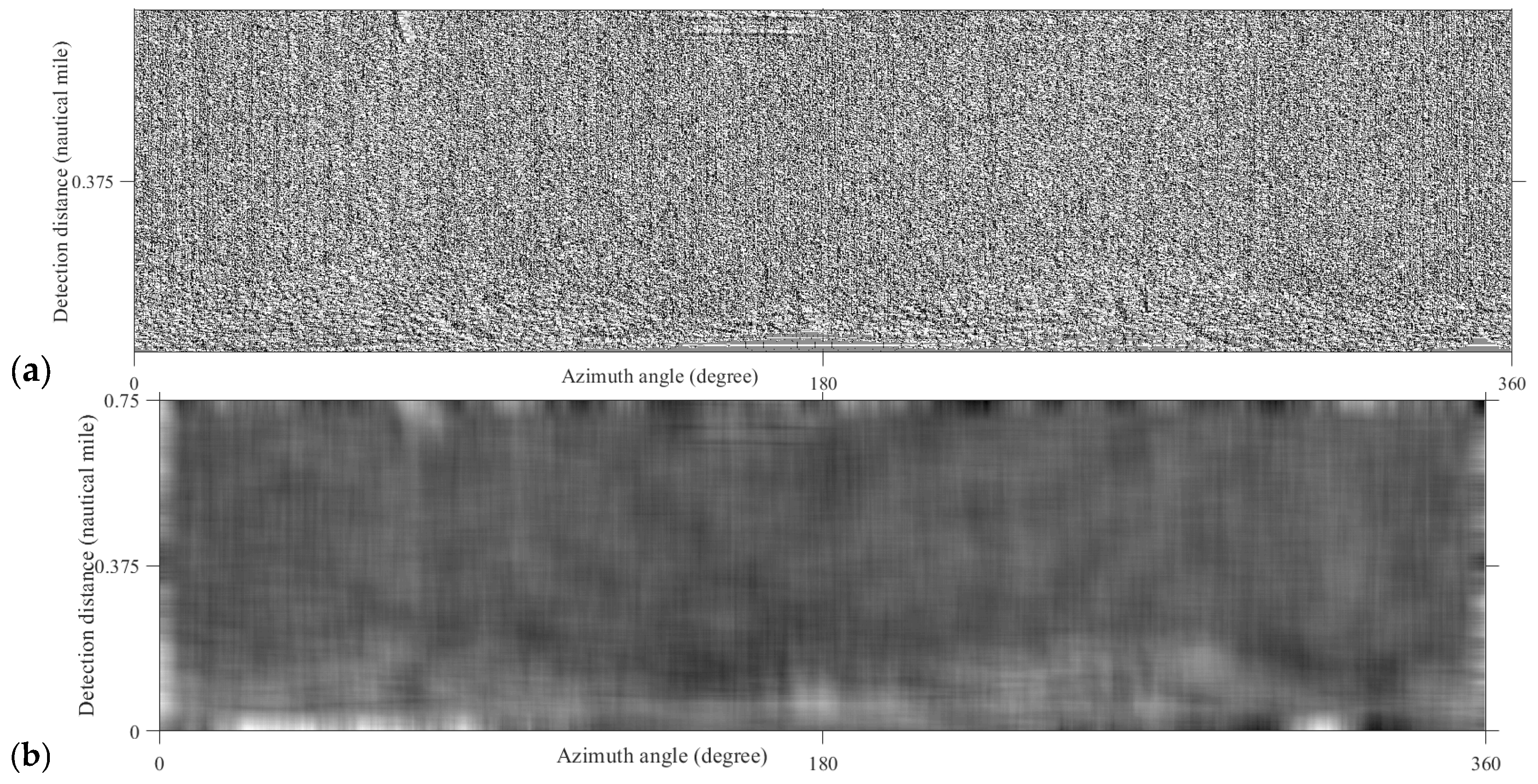
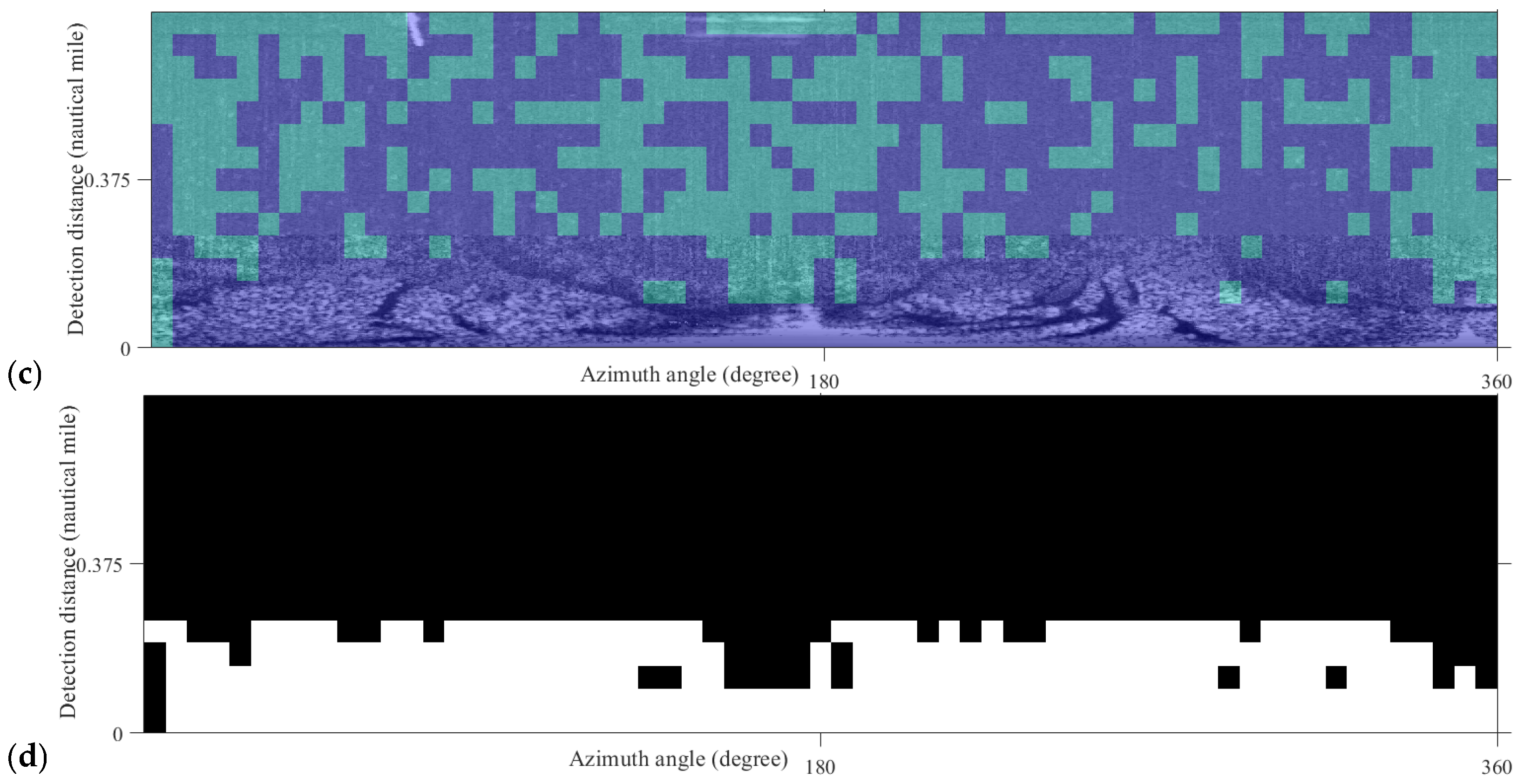
The LBP feature was extracted from the preprocessed oil spill image, as shown in Figure 10a. Then, the acquired LBP feature map was subjected to a mean filtering procedure. During this operational stage, a mean filter window was configured to the size of 64 × 64 pixels, as shown in Figure 10b. Subsequently, the HOG features were extracted from the mean-filtered LBP feature image. Thereafter, K-means clustering analysis was conducted on the extracted HOG features, as shown in Figure 10c. During this procedure, the HOG cell size was defined as 8 × 8 pixels. The HOG block size was specified as 2 × 2 pixels. The quantity of HOG direction bins was determined to be 4. Given that the image had undergone local contrast enhancement treatment, a portion of the upper area of the image was eliminated. Afterwards, a mask image delineating the ROIs was produced, as shown in Figure 10d.

3.2. Oil Film Segmentation

Once the ROIs had been extracted, preprocessed images were subjected to classification via the IFA model. The images were partitioned into four distinct categories through three-threshold classification approach. These categories were designated as the high-confidence oil films, the low-confidence oil films, the uncertain non-oil films, and the high-confidence non-oil films. The number of fireflies was 50, the maximum number of iterations was 100, the randomness parameter α was set to 0.2, the initial attraction was 1, and the light absorption coefficient was 0.5. Among these parameters, α was employed to control the random steps involved in firefly movement. When α was set to a smaller value, it guaranteed that the search process was predominantly refined locally, thereby preventing algorithm instability or convergence issued stemming from excessive randomness. If α was too large, fireflies would excessively random walk and may skip the optimal solution. If α was too small, the algorithm might fall into local optima. The setting of 100 iterations was employed to strike a balance between computational efficiency and convergence.
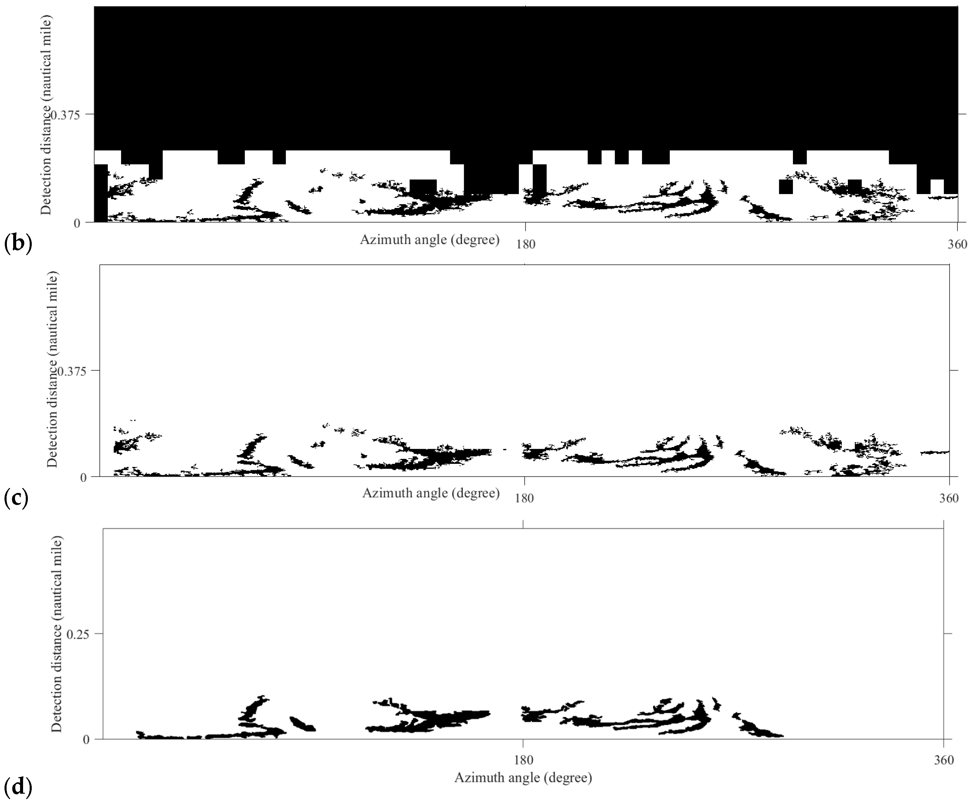
The high-confidence oil films were designated here as the real ones, as shown in Figure 11a. After that, logical operations on the ROIs mask map and the IFA model classification result were performed, as shown in Figure 11b. And the outcome was achieved as shown in Figure 11c. The result of visual interpretation was shown in Figure 11d. Nevertheless, errors are inevitably introduced when marking the oil film edges. The IFA model, an automated computational approach, was typically capable of achieving precise segmentation of the oil film target edges. Compared with the visual interpretation method, the proposed method obtained the accuracy rate of 96.77%, the recall rate of 96.82%, and the F1 score of 98.31%.
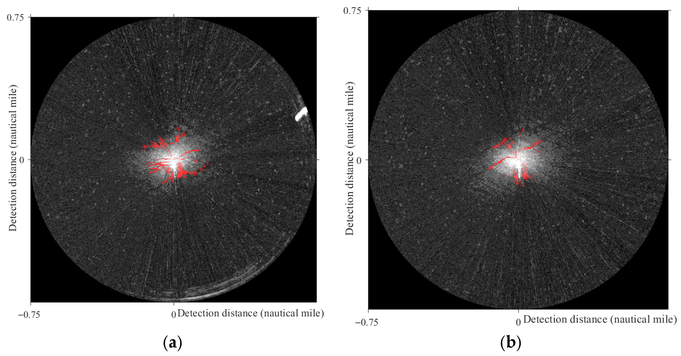
The real oil film targets were incorporated into the Polar coordinate system with red color, as shown in Figure 12.

4. Discussion

4.1. Comparation with Another Effective Oil Spill Monitoring Region Extraction Method

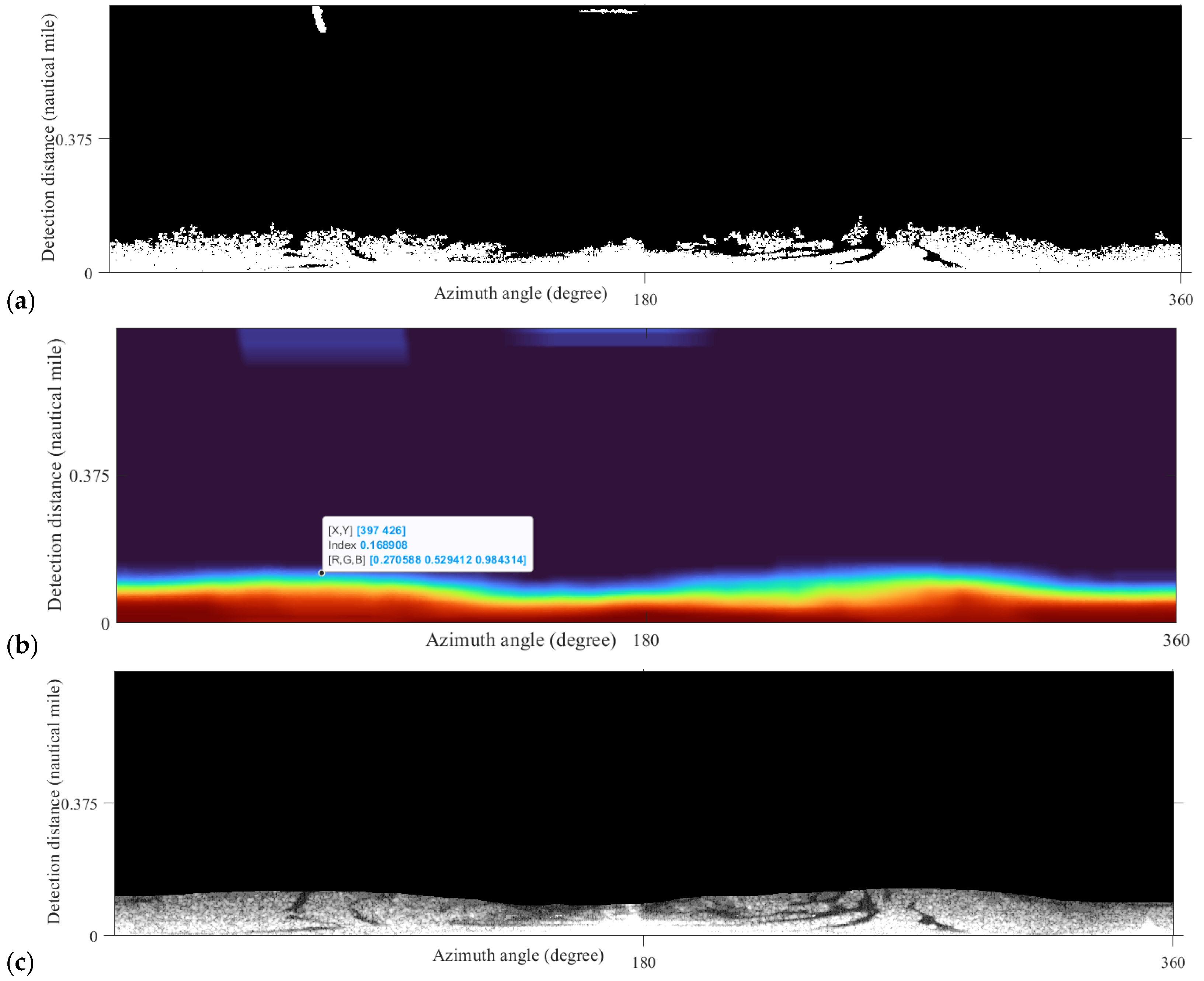
Xu et al. proposed a shipborne radar oil film detection scheme based on SVM and an improved adaptive threshold (called Method 1 here) [26]. Method 1 initially employed SVM and a grayscale distribution matrix to filter out the effective monitoring regions (ROIs) that encompassed wave pixels surrounding the vessel. Subsequently, a local adaptive thresholding technology was utilized to precisely extract the offshore oil films. Method 1 was used here to get the effective oil spill monitoring region outcomes derived from the identical denoised image (Figure 6), as shown in Figure 8. Initially, the SVM was applied for the classification between wave pixels and background components, as shown in Figure 13a. Subsequently, a grayscale distribution matrix was generated, and the segmentation threshold was manually set, as shown in Figure 13b. The threshold value in Figure 13b was required to be manually selected according to expert experience for filtering out the effective wave regions, as shown in Figure 13c. Varying thresholds would result in distinct outcomes in oil film detection. It could be clearly observed that many oil film targets had not been effectively detected in Figure 13c, meaning significant missed detections would appear. If the threshold was manually selected again at 0.3967, more oil film targets would be lost as Figure 13d. Through the comparative analysis, it became evident that our proposed method exhibited superior precision and intelligence in the ROIs extraction. Moreover, the drawbacks of subjectivity and instability inherent in the conventional manual threshold selection procedure were effectively circumvented.

4.2. Comparison of Different Filtering Methods in Effective Oil Spill Monitoring Region Extraction

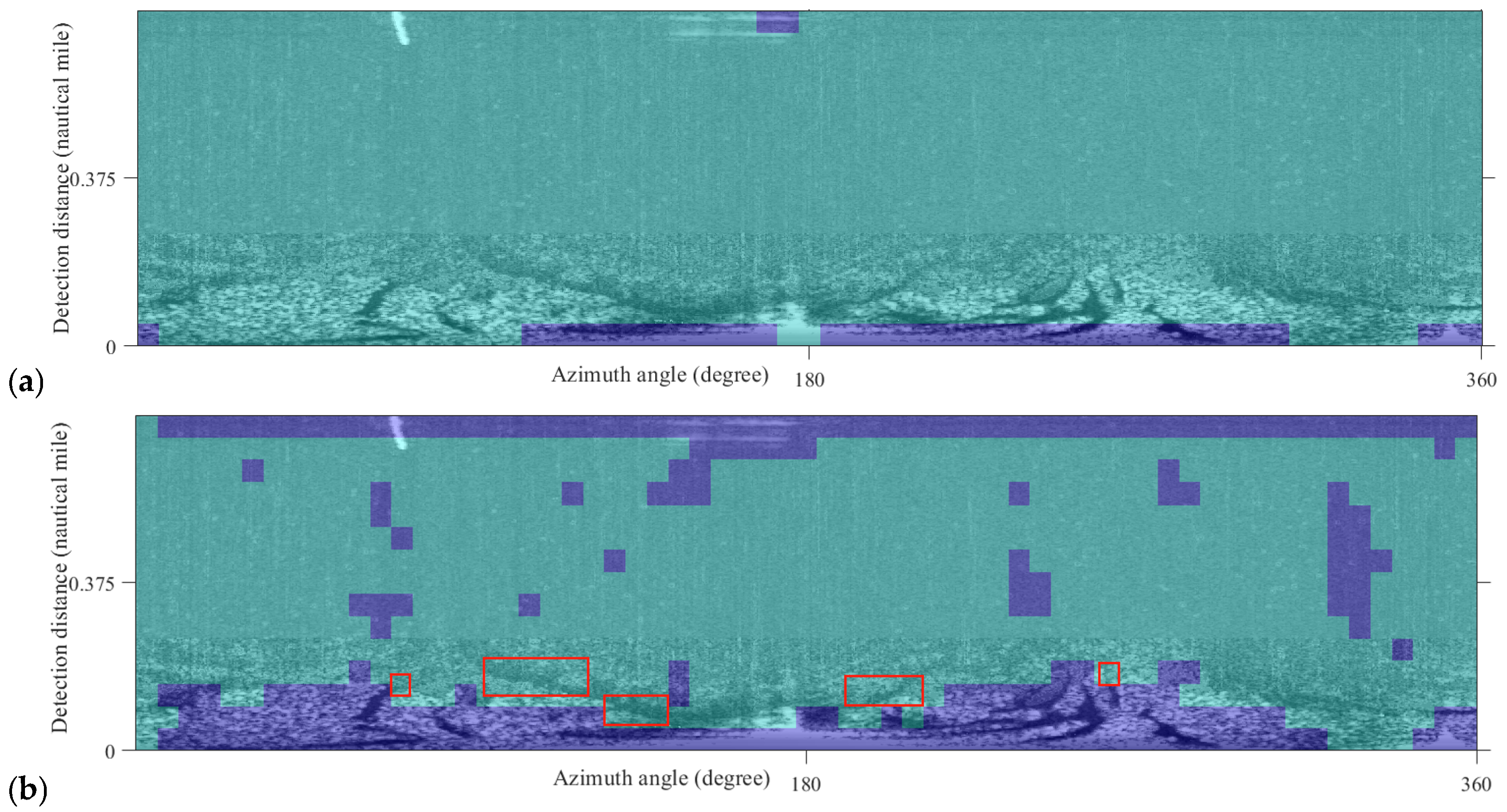
As delineated in Section 2.3, a mean filter was adopted to process the LBP features. Besides mean filter, two other approaches, including mode filter and median filter, were also available for selection, as shown in Figure 14. It was distinctly observed that the classification performance of mode filter was the poorest, with merely a minuscule quantity of oil film targets being identified. Conversely, the classification performance achieved by median filter was better, surpassing that of mode filtering. Nevertheless, a certain number of oil film targets remained undetected in red rectangles of Figure 14b. Therefore, it was recommended to use mean filter to smooth the LBP features for obtaining better effective oil spill monitoring regions.

4.3. Comparison of Another Marine Radar Oil Spill Detection Method

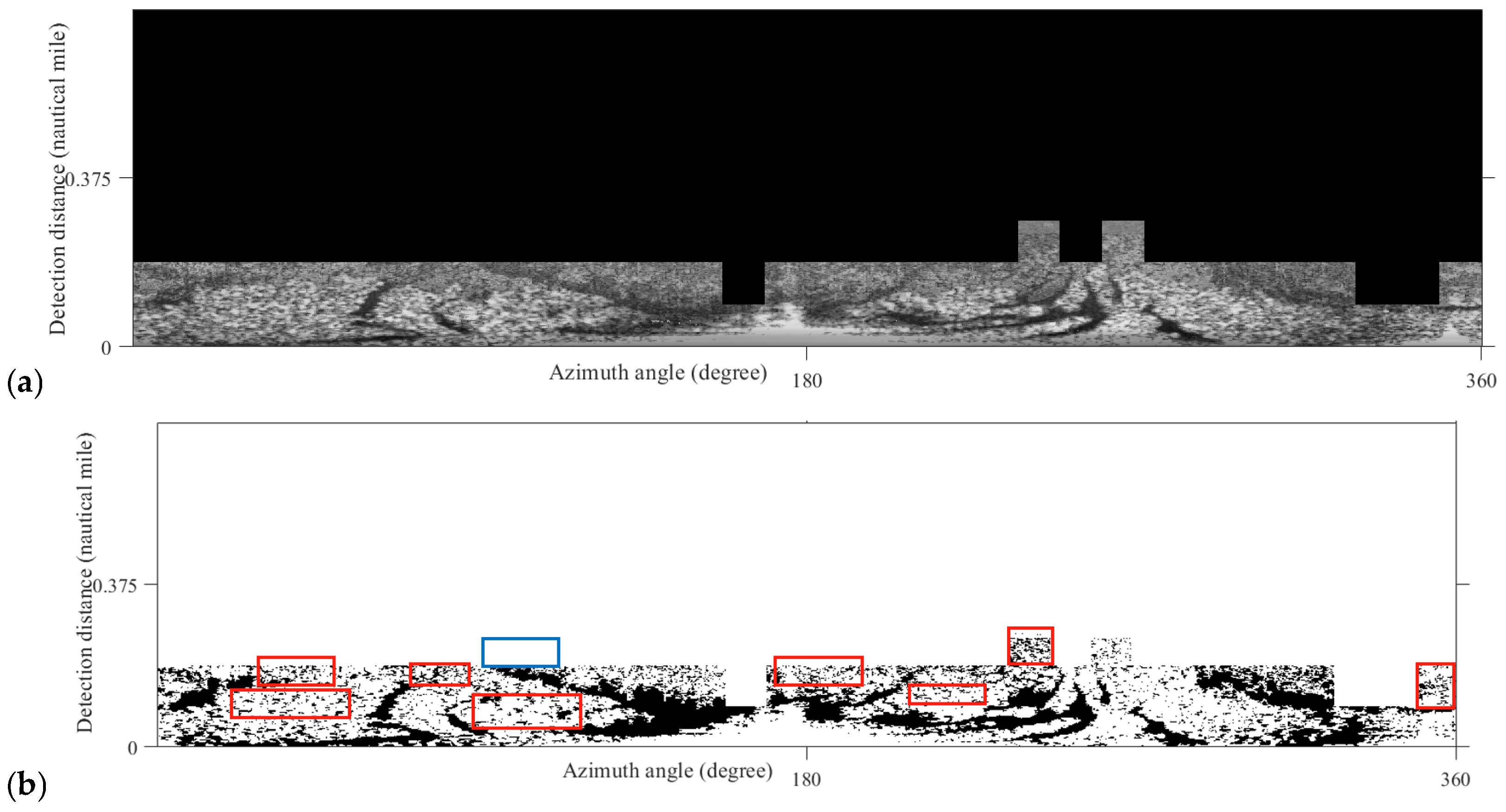
Li et al. put forward an oil spill identification approach (called Method 2 here) that integrated GLCM texture features with SVM classifier for obtaining ROIs [32]. Leveraging the ROIs, the preprocessed image was subjected to classification via the FCM algorithm here for comparison, as shown in Figure 15. Analysis of experimental results revealed that Method 2 demonstrated outstanding performance in identifying effective monitoring regions. Nonetheless, Method 2 exhibited certain constraints. During the image classification phase, a substantial number of suspected oil film targets were misclassified as authentic targets in red rectangles of Figure 15b, giving rise to scenarios of false detection. There were also some missed oil film targets in the blue rectangle. However, our proposed method showed superiority in oil film segmentation results.

4.4. Comparison with the Traditional FA Model

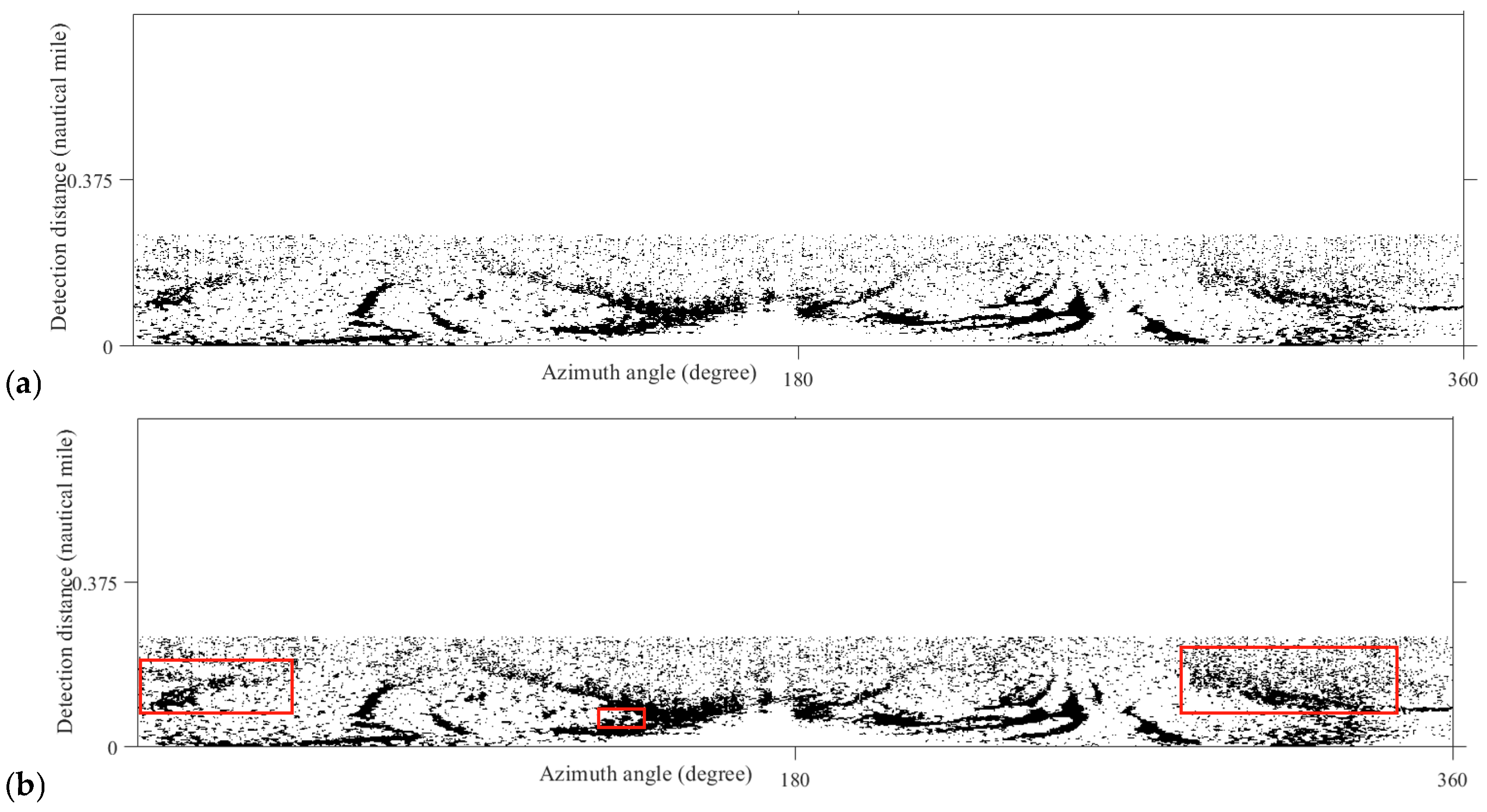
As delineated in Section 2.6, the IFA model has been employed here to segment oil spills preliminarily. The high confidence oil film classification results of the IFA model and the traditional FA model were shown in Figure 16. Through comparative analysis, it was observed that the traditional FA model misclassified numerous suspected oil films as real oil films (marked in red rectangles). The traditional FA model was distinguished by its uncomplicated and intuitive underlying principle, potent global optimization capability, less parameter count, straightforward implementation process, and broad applicability to diverse continuous optimization problems. Nevertheless, its limitation was manifested in its susceptibility to being trapped in local optimal solutions, particularly when addressing high-dimensional or multimodal issues, resulting in a sluggish convergence pace. Through the incorporation of adaptive parameter tuning, a more intricate fitness function, and boundary-handling optimization, the IFA model had its performance substantially boosted in image multi-threshold segmentation. Its local search capability and the diversity of solutions were notably strengthened. Meanwhile, ineffective solutions were circumvented by means of constraints. The oil film segmentation accuracy of the traditional FA model was 71.26%, which was lower than the IFA model. This disparity indicates that the IFA model surpassed the traditional FA model in its capacity to accurately recognize the authentic oil films.

4.5. The Challenge of Calm and Harsh Waves

Various sea conditions exert differing effects on the efficacy of maritime radar in identifying oil spills. The calm sea surface, characterized by relatively minor fluctuations in wave height and frequency, presents significant challenges for the detection of oil films via marine radar systems. In such serene conditions, the radar signals interact with the sea surface in a manner that makes it arduous to distinguish the subtle differences in backscattering caused by the presence of an oil film. Oil films on the water surface typically alter the roughness characteristics of the sea, which in turn affects the radar cross-section and the strength of the returned signals. However, when the sea is calm, the natural variability of the water surface is already quite low, and the impact of the oil film on this variability is often masked, resulting in a reduced ability to detect the oil film accurately.
Conversely, when the waves are harsh, characterized by high wave heights, steep wave slopes, and a complex wave spectrum, the oil film exhibits a weak suppression effect on the waves. The dynamic interaction between the oil film and the rough sea surface is complex. Under harsh wave conditions, the energy of the waves is substantial, and the oil film, which has a relatively low viscosity and surface tension compared to the water, is unable to effectively dampen the wave motion. As a result, the radar signatures of the oil-covered and oil-free areas of the sea surface become less distinct. The weak suppression effect leads to a situation where the oil film does not significantly modify the wave-induced backscattering patterns, making it difficult for marine radar to identify the presence of oil spills based on the analysis of these patterns. This, in turn, increases the overall difficulty of detecting oil spills in marine radar Consequently, specific datasets, customized for each sea condition, are imperative for training and enhancing corresponding algorithms. To tackle this challenge, marine radar data encompassing diverse sea conditions and multiple oil types must be persistently and broadly gathered.

5. Conclusions

In this study, a novel approach for marine oil spill detection was put forward. Initially, the raw oil spill radar data underwent pre-processing. Subsequently, it was processed by employing LBP feature, mean filter, and HOG feature. After that, K-Means classification was carried out for the successful extraction of ROIs. Ultimately, an IFA model was applied for the accurate extraction of oil spills.
The FA is extensively applied to a variety of optimization problems owing to its straightforward architecture, robust global search capability, and facile implementation. Nevertheless, when utilized for oil-film segmentation in marine radar data, it is merely capable of roughly pinpointing the oil film targets. The proposed IFA model here can achieve a notable improvement in segmentation precision while preserving its inherent advantage in global search. It proves to be highly effective in extracting the low-contrast oil films within radar imagery. Moreover, the method adopted in this research exhibits automation traits. It can efficiently preclude the errors and subjective disruptions stemming from manual handling, thereby guaranteeing the objectivity and scientific rigor of the ultimate outcomes. However, the dynamic parameter adjustment mechanism of this algorithm may lead to an increase in computational complexity. The multi-group collaboration mode is strongly reliant on parallel computing resources. Regarding potential application, the algorithm can be adjusted for applying to highlight target segmentation in unmanned aerial vehicle (UAV) images.
In order to improve the applicability of marine radar oil spill detection in different sea conditions, high-quality oil spill image data will be generated by leveraging the adversarial training mechanism of generators and discriminators within Generative Adversarial Networks (GANs) In forthcoming research.

Author Contributions

Conceptualization, J.X. and B.Y.; methodology, H.D. and Z.G.; software, B.X. and J.X.; validation, Y.H. and B.L. (Bo Li); resources, J.X., S.Q. and B.L. (Bingxin Liu); data curation, J.X.; writing—original draft preparation, B.Y.; writing—review and editing, J.X. and B.Y.; supervision, J.X. and H.D.; project administration, J.X.; funding acquisition, J.X. and H.D. All authors have read and agreed to the published version of the manuscript.

Funding

This research was funded by the Guangdong Basic and Applied Basic Research Foundation, grant numbers 2025A1515010886, 2023A1515011212, National Natural Science Foundation of China, grant number 52271359, the Special Projects in Key Fields of Ordinary Universities in Guangdong Province, grant number 2022ZDZX3005, the Shenzhen Science and Technology Program, grant number JCYJ20220530162200001, Postgraduate Education Innovation Project of Guangdong Ocean University, grant numbers 202421, 202539, 202551, Fund of Guangdong Provincial Key Laboratory of Intelligent Equipment for South China Sea Marine Ranching, Grant NO. 2023B1212030003.

Conflicts of Interest

The authors declare that they have no known competing financial interests.

References

  1. Ji, H.; Wang, T.; Wang, Y.; Yang, K.; Jiang, J.; Xing, Z. Influence and Prediction of Oil Film Migration in Submarine Pipeline Spills under Multiple Factors. Process Saf. Environ. Prot. 2023, 178, 74–86. [Google Scholar] [CrossRef]
  2. Chen, Y.; Zhou, S.; Yu, W.; Hu, H. A Novel Environment-Adaptive Dual-Light Image Enhancement Framework for Marine Oil Spill Detection. Mar. Pollut. Bull. 2024, 209, 117257. [Google Scholar] [CrossRef]
  3. Sun, Z.; Yang, Q.; Yan, N.; Chen, S.; Zhu, J.; Zhao, J.; Sun, S. Utilizing Deep Learning Algorithms for Automated Oil Spill Detection in Medium Resolution Optical Imagery. Mar. Pollut. Bull. 2024, 206, 116777. [Google Scholar] [CrossRef]
  4. Scarlett, A.G.; Nelson, R.K.; Gagnon, M.M.; Reddy, C.M.; Grice, K. Very Low Sulfur Fuel Oil Spilled from the MV Wakashio in 2020 Remains in Sediments in a Mauritius Mangrove Ecosystem Nearly Three Years after the Grounding. Mar. Pollut. Bull. 2024, 209, 117283. [Google Scholar] [CrossRef]
  5. Boesch, D.F.; Cebrian, J.; Fonseca, V.F.; Landers, S.C.; Marshall, N.J. Editorial: Vulnerability and Resilience of Marine Ecosystems Affected by the Deepwater Horizon Oil Spill. Front. Mar. Sci. 2023, 10, 1253605. [Google Scholar] [CrossRef]
  6. Lau, T.-K.; Huang, K.-H. A Timely and Accurate Approach to Nearshore Oil Spill Monitoring Using Deep Learning and GIS. Sci. Total Environ. 2024, 912, 169500. [Google Scholar] [CrossRef] [PubMed]
  7. Freeman, D.H.; Nelson, R.K.; Pate, K.; Reddy, C.M.; Ward, C.P. Forecasting Photo-Dissolution for Future Oil Spills at Sea: Effects of Oil Properties and Composition. Environ. Sci. Technol. 2024, 58, 15236–15245. [Google Scholar] [CrossRef] [PubMed]
  8. Bui, N.A.; Oh, Y.; Lee, I. Oil Spill Detection and Classification through Deep Learning and Tailored Data Augmentation. Int. J. Appl. Earth Obs. Geoinf. 2024, 129, 103845. [Google Scholar] [CrossRef]
  9. Chen, Y.-T.; Chang, L.; Wang, J.-H. Full-Scale Aggregated MobileUNet: An Improved U-Net Architecture for SAR Oil Spill Detection. Sensors 2024, 24, 3724. [Google Scholar] [CrossRef]
  10. Zapata-Peñasco, I.; Avelino-Jiménez, I.A.; Mendoza-Pérez, J.; Vázquez Guevara, M.; Gutiérrez-Ladrón de Guevara, M.; Valadez-Martínez, M.; Hernández-Maya, L.; Garibay-Febles, V.; Fregoso-Aguilar, T.; Fonseca-Campos, J. Environmental Stressor Assessment of Hydrocarbonoclastic Bacteria Biofilms from a Marine Oil Spill. Biotechnol. Rep. 2024, 42, e00834. [Google Scholar] [CrossRef]
  11. Jiao, J.; Lu, Y.; Hu, C. Characterizing Oil Spills Using Deep Learning and Spectral-Spatial-Geometrical Features of HY-1C/D CZI Images. Remote Sens. Environ. 2024, 308, 114205. [Google Scholar] [CrossRef]
  12. Brekke, C.; Solberg, A.H.S. Oil Spill Detection by Satellite Remote Sensing. Remote Sens. Environ. 2005, 95, 1–13. [Google Scholar] [CrossRef]
  13. Fan, J.; Zhang, S.; Wang, X.; Xing, J. Multifeature Semantic Complementation Network for Marine Oil Spill Localization and Segmentation Based on SAR Images. IEEE J. Sel. Top. Appl. Earth Obs. Remote Sens. 2023, 16, 3771–3783. [Google Scholar] [CrossRef]
  14. Chen, G.; Huang, J.; Wen, T.; Du, C.; Lin, Y.; Xiao, Y. Multiscale Feature Fusion for Hyperspectral Marine Oil Spill Image Segmentation. J. Mar. Sci. Eng. 2023, 11, 1265. [Google Scholar] [CrossRef]
  15. Yang, J.; Wang, J.; Hu, Y.; Ma, Y.; Li, Z.; Zhang, J. Hyperspectral Marine Oil Spill Monitoring Using a Dual-Branch Spatial–Spectral Fusion Model. Remote Sens. 2023, 15, 4170. [Google Scholar] [CrossRef]
  16. Ren, P.; Jia, Q.; Xu, Q.; Li, Y.; Bi, F.; Xu, J.; Gao, S. Oil Spill Drift Prediction Enhanced by Correcting Numerically Forecasted Sea Surface Dynamic Fields with Adversarial Temporal Convolutional Networks. IEEE Trans. Geosci. Remote Sens. 2025, 63, 4701018. [Google Scholar] [CrossRef]
  17. Akhmedov, F.; Nasimov, R.; Abdusalomov, A. Developing a Comprehensive Oil Spill Detection Model for Marine Environments. Remote Sens. 2024, 16, 3080. [Google Scholar] [CrossRef]
  18. Prajapati, K.; Bhavsar, M.; Mahajan, A. GSCAT-UNET: Enhanced U-Net Model with Spatial-Channel Attention Gate and Three-Level Attention for Oil Spill Detection Using SAR Data. Mar. Pollut. Bull. 2025, 212, 117583. [Google Scholar] [CrossRef]
  19. Chen, R.; Li, B.; Jia, B.; Xu, J.; Ma, L.; Yang, H.; Wang, H. Oil Spill Identification in X-Band Marine Radar Image Using K-Means and Texture Feature. PeerJ Comput. Sci. 2022, 8, e1133. [Google Scholar] [CrossRef]
  20. Liu, P.; Liu, B.; Li, Y.; Chen, P.; Xu, J. Oil Spill Detection on X-Band Marine Radar Images Based on Sea Clutter Fitting Model. Heliyon 2023, 9, e20893. [Google Scholar] [CrossRef]
  21. Shen, J.; Han, B.; Pan, Z.; Li, G.; Hu, Y.; Ding, C. Learning Time–Frequency Information with Prior for SAR Radio Frequency Interference Suppression. IEEE Trans. Geosci. Remote Sens. 2022, 60, 5239716. [Google Scholar] [CrossRef]
  22. Liu, X.; Cheung, G.; Wu, X. Joint Denoising and Contrast Enhancement of Images Using Graph Laplacian Operator. In Proceedings of the 2015 IEEE International Conference on Acoustics, Speech and Signal Processing (ICASSP), South Brisbane, Australia, 19–24 April 2015. [Google Scholar]
  23. Xu, X.; Xu, S.; Jin, L.; Song, E. Characteristic Analysis of Otsu Threshold and Its Applications. Pattern Recognit. Lett. 2011, 32, 956–961. [Google Scholar] [CrossRef]
  24. Jaybhay, J.; Shastri, R. A Study of Speckle Noise Reduction Filters. Signal Image Process. 2015, 6, 71–80. [Google Scholar] [CrossRef]
  25. Zhang, L.; Jin, H.; Wu, D. Analysis and Comparison of Grayscale Correction. In Proceedings of the 3rd International Conference on Robotics, Control and Automation, Chengdu, China, 11–13 August 2018; pp. 180–184. [Google Scholar]
  26. Xu, J.; Wang, H.; Cui, C.; Zhao, B.; Li, B. Oil Spill Monitoring of Shipborne Radar Image Features Using SVM and Local Adaptive Threshold. Algorithms 2020, 13, 69. [Google Scholar] [CrossRef]
  27. Ariateja, D.; Ardiyanto, I.; Soesanti, I. A Review of Contrast Enhancement Techniques in Digital Image Processing. In Proceedings of the 2018 4th International Conference on Science and Technology (ICST), Yogyakarta, Indonesia, 7–8 August 2018. [Google Scholar]
  28. Song, K.-C.; Yan, Y.-H.; Chen, W.-H.; Zhang, X. Research and Perspective on Local Binary Pattern. Acta Autom. Sin. 2013, 39, 730–744. [Google Scholar] [CrossRef]
  29. Ren, H.; Li, Z.-N. Object Detection Using Edge Histogram of Oriented Gradient. In Proceedings of the 2014 IEEE International Conference on Image Processing (ICIP), Paris, France, 27–30 October 2014. [Google Scholar]
  30. Likas, A.; Vlassis, N.; Verbeek, J.J. The Global K-Means Clustering Algorithm. Pattern Recognit. 2003, 36, 451–461. [Google Scholar] [CrossRef]
  31. Wu, J.; Wang, Y.-G.; Burrage, K.; Tian, Y.-C.; Lawson, B.; Ding, Z. An Improved Firefly Algorithm for Global Continuous Optimization Problems. Expert Syst. Appl. 2020, 149, 113340. [Google Scholar] [CrossRef]
  32. Li, B.; Xu, J.; Pan, X.; Ma, L.; Zhao, Z.; Chen, R.; Liu, Q.; Wang, H. Marine Oil Spill Detection with X-Band Shipborne Radar Using GLCM, SVM and FCM. Remote Sens. 2022, 14, 3715. [Google Scholar] [CrossRef]
Figure 1. Data acquisition device architecture.
Remotesensing 17 03148 g001
Figure 2. Original marine radar image.
Remotesensing 17 03148 g002
Figure 3. The data pre-processing.
Remotesensing 17 03148 g003
Figure 4. The original image in Cartesian coordinate system.
Remotesensing 17 03148 g004
Figure 5. Co-frequency interference denoising image.
Remotesensing 17 03148 g005
Figure 6. Spot suppression image.
Remotesensing 17 03148 g006
Figure 7. Grayscale global adjustment image.
Remotesensing 17 03148 g007
Figure 8. Local contrast enhanced image.
Remotesensing 17 03148 g008
Figure 9. Calculation process of LBP eigenvalue.
Remotesensing 17 03148 g009
Figure 10. ROIs extraction. (a) The LBP feature map; (b) The mean filtering; (c) K-means clustering; (d) The Oil film ROIs mask image.
Remotesensing 17 03148 g010aRemotesensing 17 03148 g010b
Figure 11. Oil film segmentation. (a) High-confidence oil film classification results. (b) Logical operations with the ROIs mask map. (c) Final result. (d) Result of visual interpretation.
Remotesensing 17 03148 g011aRemotesensing 17 03148 g011b
Figure 12. Results in Polar coordinate system. The oil film targets were marked in red color. (a) Experimental data. (b) Another oil spill image.
Remotesensing 17 03148 g012
Figure 13. The effective ocean wave monitoring scope of Method 1. (a) SVM classification of ocean wave; (b) The threshold was manually set to 0.1689. (c) The ocean wave monitoring range segmentation of threshold 0.1689. (d) The threshold was manually set to 0.3967. (e) The ocean wave monitoring range segmentation of threshold 0.3967.
Remotesensing 17 03148 g013aRemotesensing 17 03148 g013b
Figure 14. Classification results of different filter methods in effective oil spill monitoring region extraction. (a) Mode filter. (b) Median filter.
Remotesensing 17 03148 g014
Figure 15. Oil spill detection results based on Method 2. (a) Effective oil spill monitoring regions; (b) FCM classification results in effective monitoring regions.
Remotesensing 17 03148 g015
Figure 16. Comparison with the traditional FA model. (a) The IFA classification result. (b) The traditional FA classification result.
Remotesensing 17 03148 g016
Table 1. Marine radar technical parameters.
Parameter NameParameter Value
Distance resolution3.75 M
Antenna length8 FT
Polarization modeHorizontal Polarization
Rotation speed28–45 RPM
Peak power25 KW
Detection angleHorizontal: 0–360°; Vertical: 0–25°
Pulse repetition rate3000 Hz/1800 Hz/785 Hz
Disclaimer/Publisher’s Note: The statements, opinions and data contained in all publications are solely those of the individual author(s) and contributor(s) and not of MDPI and/or the editor(s). MDPI and/or the editor(s) disclaim responsibility for any injury to people or property resulting from any ideas, methods, instructions or products referred to in the content.