Article

Differential Urban-Rural Inequalities and Driving Mechanisms of PM2.5 Exposure in the Central Plains Urban Agglomeration, China

1
State Key Laboratory of Environmental Criteria and Risk Assessment, Chinese Research Academy of Environmental Sciences, Beijing 100012, China
2
College of Forestry, Northeast Forestry University, Harbin 150040, China
3
Key Laboratory of Sustainable Forest Ecosystem Management-Ministry of Education, Northeast Forestry University, Harbin 150040, China
4
Research and Development Center of Big Data for Ecosystem, Northeast Forestry University, Harbin 150040, China
5
College of Environmental Science and Engineering, Nankai University, Tianjin 300350, China
6
State Environmental Protection Key Laboratory of Urban Ambient Air Particulate Matter Pollution Prevention and Control, Tianjin 300350, China
7
College of Materials and Energy, Lanzhou University, Lanzhou 730137, China
8
College of Underwater Acoustic Engineering, Harbin Engineering University, Harbin 150006, China
*
Author to whom correspondence should be addressed.
Remote Sens. 2025, 17(17), 2982; https://doi.org/10.3390/rs17172982
Submission received: 13 July 2025 / Revised: 17 August 2025 / Accepted: 25 August 2025 / Published: 27 August 2025

Abstract

Exposure to PM2.5 poses severe risks to public health and sustainable development, with exposure inequalities exacerbated by variations in atmospheric activity and uneven regional development. However, the urban-rural inequalities and natural-human driving mechanisms underlying PM2.5 exposure inequalities within urban agglomerations are poorly understood. Taking the Central Plains Urban Agglomeration (CPUA) in China as an example, this study investigated the spatio-temporal variations of PM2.5 and considered its future trends. The Theil index was employed to quantify PM2.5 exposure inequalities. An interpretable machine learning model (RF-SHAP) was applied to identify the raster natural and socioeconomic driving factors. We found that 99.68% of the CPUA exhibited a decreasing trend in ground-level PM2.5. The overall Theil index decreased from 0.168 to 0.142, with a rural decline from 0.115 to 0.084, suggesting an overall reduction in air pollution inequalities, particularly in rural areas. Conversely, the urban Theil index increased from 0.096 to 0.208, highlighting an increasing inequality in urban PM2.5 exposure. Resource-based cities, such as Changzhi, Jincheng, and Jiaozuo, exhibited the largest PM2.5 exposure inequality. Elevation was identified as the dominant factor influencing overall and rural PM2.5 exposure inequalities, while population density was the primary driver of urban inequalities. This study highlighted the differences in urban−rural PM2.5 inequalities and their drivers at the city agglomeration scale. The aims were to mitigate PM2.5 exposure inequalities through socio-environmental systems, provide evidence for the integrated management of PM2.5 exposure inequalities in city agglomerations, and support regional sustainable development.

1. Introduction

Atmospheric particulate matter with an aerodynamic diameter of less than or equal to 2.5 μm (PM2.5) is the primary contributor to air pollution events, such as haze [1]. Prolonged exposure to PM2.5 significantly increases the risk of cardiovascular, cerebrovascular, and respiratory diseases, thereby diminishing life expectancy in affected populations [2]. Various types of particles, including vehicle exhaust emissions and fugitive dust, exacerbate the PM2.5 exposure inequalities between urban and rural areas [3,4]. This imbalance has hampered progress toward achieving the Sustainable Development Goals (SDGs) [5,6,7,8,9]. With the increasing pace of urbanization, the sources of PM2.5 have become increasingly diverse, regional, and complicated, and PM2.5 concentrations are influenced by climate conditions, geographic characteristics, pollution control technology and management, and socio-economic factors. Identifying emission sources and reducing PM2.5 emissions, as well as implementing regional joint prevention measures, are critical strategies for improving air quality and promoting regional equity. The success of these measures in safeguarding public health and human well-being requires a comprehensive understanding of the urban−rural PM2.5 exposure inequalities and their underlying drivers [7,10].
Several studies have explored the factors driving air pollution across varying scales. At the urban scale, meteorological datasets have been widely applied to assess the climate influences on air pollution over daily, monthly, and annual periods [11,12]. Atmospheric chemical transport models have been used during the critical pollution seasons to trace particulate matter sources and facilitate the precise attribution of pollutant exposure within localized regions [13]. On broader regional scales, studies have examined the socio-economic drivers of particulate pollution, explored the ‘urban pollution island’ effect, and developed strategies for their integrated management [14,15,16]. Rapid economic growth, coupled with inadequate pollution control measures, amplifies air pollution exposure, endangering public health and ecological stability [5,8]. Therefore, identifying effective pathways for mitigating and controlling air pollution, based on a comprehensive understanding of its drivers, remains a research priority.
The inequalities of air pollution exposure among different regions have received increasing attention from researchers. Addressing these inequalities, particularly amidst the ongoing economic expansion in China, is vital for improving human well-being [17,18,19]. Advanced geospatial analyses have quantitatively assessed exposure inequalities from the street to global scales, uncovering how inequalities in pollution exposure correlate with negative health outcomes, including mortality [7,20,21,22,23,24]. Additionally, studies have linked these inequalities to socio-environmental determinants such as economic development and climate change, highlighting the complex interplay between environmental exposure, health inequities, and regional development. These studies have developed strategies for advancing environmental equity and managing air pollution across regions [25,26,27]. However, the differences in PM2.5 exposure inequality between urban and rural areas over a long period of time still need to be further clarified to reduce the inequality in development urban agglomeration between urban and rural areas.
Several critical research gaps have been identified. First, there is a need to explore the spatio-temporal patterns and future trends of air pollution in urban agglomerations to identify governance hotspots. Second, the long-term evolution of urban−rural PM2.5 exposure inequality in developing countries remains poorly understood, especially in the context of policy constraints and rapid urbanization. While previous studies have examined PM2.5 exposure inequalities, few have integrated natural, climate, emission-related, and socio-economic factors to analyze urban−rural inequalities comprehensively [28].
This study investigated urban−rural PM2.5 exposure inequalities within China, with an emphasis on the Central Plains Urban Agglomeration (CPUA). The CPUA is a densely populated region undergoing rapid urbanization and industrialization, thus facing significant air pollution challenges. The CPUA includes the Taihang Mountains, which influence the transport of air pollutants, leading to high levels of air pollution in this area. Furthermore, the region is characterized by a dense population and the presence of heavy industries, particularly in the northern CPUA, where the abundant coal resources exacerbate vulnerabilities in human well-being [29]. Given its distinctive natural environment and relatively slow pace of socio-economic development, the CPUA was selected as a case study to precisely identify the socio-economic and environmental drivers behind urban−rural PM2.5 exposure inequalities under complex terrain and climate conditions. The findings were used to develop a model for managing PM2.5 exposure inequalities in densely populated, industrialized regions and to promote integrated management strategies at the urban agglomeration scale. By investigating the spatio-temporal patterns of PM2.5 pollution and urban−rural exposure inequalities within the CPUA, the study aimed to identify priority governance zones for air pollution management and proposed scientifically grounded pathways for their integrated management. The research directly aligned with SDG 3 (Good health and well-being), SDG 10 (Reduced inequalities), and SDG 11 (Sustainable cities and communities) [9,30,31,32]. The study addressed three core research questions: (1) How have the spatial and temporal patterns of PM2.5 pollution evolved within representative urban agglomerations, and what insights can be derived from forecasting future trends and identifying pollution hotspots? (2) What are the dynamics of urban−rural PM2.5 exposure inequalities within urban agglomerations, and how have they changed over time? (3) How do natural, climate, and socio-economic drivers collectively influence urban−rural exposure inequalities, and what strategies can be proposed for effective mitigation?

2. Research Methods

2.1. Research Area

Figure 1 shows the location of the CPUA in China, encompassing 30 prefecture-level cities and extends across five provincial-level administrative divisions: Henan, Shandong, Anhui, Shanxi, and Hebei (Figure 1a,b). The CPUA exemplifies a typical case of rapid urbanization and socio-economic transformation, covering approximately 287,000 km2—accounting for 2.99% of China. The CPUA has a complex topography, which is dominated by mountains in the west and plains in the east-central part, with an average elevation of about 288 m (Figure 1c). The complex topography has led to differences in regional atmospheric activity and socio-economic development. In 2022, the China Urban Statistical Yearbook showed that the CPUA contributed 6.88% of the national GDP (8485 billion yuan) and accommodated 13.32% of the total population (188.03 million) of China. The annual mean PM2.5 concentration in the CPUA is 44 μg/m3, which is 1.46 times the average PM2.5 concentration in China (30.8 μg/m3). The ratio of maximum to minimum of PM2.5 concentrations in this area is approximately 2 (Figure 1d). These data highlight a stark disparity between urban and rural areas within the CPUA regarding air pollution exposure, socio-economic conditions, and public resource distribution. As a key component of the national “Rise of Central China” strategy, the CPUA faces substantial pressure to balance economic growth and environmental protection. The region urgently requires scientific evidence to guide pollution mitigation and promote sustainable development. Studying the CPUA can offer practical insights into improving local air pollution control, while also providing a valuable reference for pollution prevention and management in similar urban agglomerations worldwide [33] (Figure 1e,f).

2.2. Data Preparation

2.2.1. PM2.5 Data

The PM2.5 data used in this study were sourced from the Big Data Seamless 1 km Ground-level PM2.5 dataset within the China High Air Pollutants (CHAP) dataset, which provides annual ground-level PM2.5 estimates from 2000 to 2023 at a spatial resolution of 1 km (https://weijing-rs.github.io/ (accessed on 25 August 2025)). This dataset integrates multi-source remote sensing data and employs a four-dimensional spatiotemporal-extreme stochastic model, combining ground-based observational data, atmospheric reanalysis data, emission inventories, and model simulations. It effectively addresses the data gaps in the Moderate Resolution Imaging Spectroradiometer (MODIS) multi-angle implementation of atmospheric correction (MAIAC) aerosol optical depth (AOD) products and exhibits a high cross-validation coefficient of determination between training and text sets (C-V R2 = 0.92), making it suitable for the long-term analysis of PM2.5 pollution trends at the urban agglomeration scale (Table 1) [34,35].

2.2.2. Urban−Rural Boundary Data

To delineate urban and rural areas and examine the inequalities in air pollution exposure within the CPUA, the study employed an annual global urban dataset based on coordinated nighttime lighting data [36]. This dataset provides long-term global urban mapping with a consistent spatial and temporal resolution (1992–2020, 1 km) matching that of the PM2.5 dataset from 2000 to 2020 based on the origin remote sensing data of DMSP-OLS and NPP-VIIRS. Due to the limited temporal resolution of the urban boundary data source, the study only analyzed the inequality of urban−rural pollution exposure in the CPUA from 2000 to 2020. It dynamically captures areas of high-intensity human activity, enabling the precise identification of urban and rural areas within the CPUA and facilitating an in-depth analysis of urban−rural PM2.5 exposure inequality (Table 1) [36]. To ensure the accuracy of city boundaries, urban areas were precisely delineated on an annual basis. The definition of urban areas was based on data sources, namely areas of human activity with continuous nighttime light intensity.

2.2.3. Control Factor Data

To explore the variability in the drivers of urban−rural PM2.5 exposure inequality, climate, emission, and socio-economic factors were investigated for five representative years: 2000, 2005, 2010, 2015, and 2020. The natural factors were vegetation cover (normalized difference vegetation index, NDVI) [37] and elevation (ELE) [38]. The climate factors were precipitation (PRE) [39] and temperature (TEM) [40]. The emission factors were ground-level PM2.5 (PM) [34,35], electricity consumption (EC) [41], and ozone concentration (O3) [42]. The socio-economic factors were nighttime lighting data (NTL) [43], population density (POP) data in a 1 × 1 km raster [44], and gross domestic production (GDP) data [45]. All control factors data have a space resolution of 1 km from 2000 to 2020. These variables were used to analyze urban−rural PM2.5 exposure inequalities and provide a foundation for integrated urban−rural air pollution management (Table 1).

2.3. Methods

2.3.1. Spatial and Temporal Trends of PM2.5 in the Central Plains Urban Agglomeration

The Sen trend analysis and Mann-Kendall (MK) test are widely applied techniques for the trend analysis of an atmospheric pollution concentration time series because they can overcome the interference from outliers or large measurement errors [46], providing more robust results than traditional methods [47]. The trend of PM2.5 exposure intensity and its statistical significance in the CPUA from 2000 to 2023 were analyzed using these two methods. The formula for calculating the Sen slope (β) is as follows [48,49,50]:
β = m e d i a n P M j P M i j i
where “median” refers to the median of the PM2.5 data series, with 1 < I < j < n; i, j represents different times; and PMi and PMi are the corresponding PM2.5 values at times i and j, respectively.
When the slope β is >0, it indicates an upward trend; when β = 0, there is no trend; and when β is <0, it means a downward trend.
The Mann-Kendall test was used to identify the year with a significant PM2.5 change. The test is based on the statistic S, which is defined as
S = i = 1 n 1 j = i + 1 n s g n = ( x j x i )
s g n x j x i = + 1     i f ( x j x i ) > 0 0     i f x j x i = 0 1     i f x j x i < 0 ,
A trend test was performed using the statistic Z. Z is calculated as follows:
Z = S V a r S   ( S > 0 )                 0                 ( S = 0 ) S + 1 V a r S ( S > 0 )
where Var is calculated as
V a r S = n ( n 1 ) ( 2 n + 5 ) 18
where n is the total number of data points in the series and ti denotes the number of data points in group i. A linkage group is a set of data with the same value.
A bilateral trend test is used to assess trends at a specific α significance level. When Z Z 1 α 2 , the null hypothesis is accepted, indicating that the trend is not significant. When Z > Z 1 α 2 , the null hypothesis is rejected, and the trend is considered significant. Three significance levels were tested: α = 0.01, α = 0.05, and α = 0.1. If the absolute value of Z exceeded 1.65, 1.96, or 2.58, the trend was considered significant at the 90%, 95%, and 99% confidence levels, respectively. In this study, the PM2.5 changes were categorized into eight levels (Table 2).

2.3.2. Predicted Changes in PM2.5 in the Central Plains Urban Agglomeration

The Hurst index (H) was employed to characterize the future trends in the PM2.5 concentration. The Hurst index is a key statistical metric that measures the persistence or self-similarity of a time series. The Hurst index is calculated as follows [51]:
First, the spatial and temporal variation sequence of PM2.5 is defined as PM(t), where t = 1, 2, 3⋯, and the mean series is defined as P M ¯ ( τ ) .
P M ¯ ( τ ) = 1 τ t = 1 τ P M t
The cumulative deviation sequence U(t,τ) is denoted as
U ( t , τ ) = t = 1 τ P M t P M τ ( 1 t τ )
The extreme deviation series (R) is
R ( τ ) = m a x 1 t τ U t , τ m i n 1 t τ U t , τ τ = 1 , 2 , 3
The standard deviation series (S) is
S ( τ ) = [ 1 τ t = 1 τ ( P M t P M ¯ ( τ ) ) 2 ] 1 2
Finally, the Hurst index is calculated as follows:
R S = R τ S τ = ( τ ) H
where H represents the Hurst index, ranging from 0 to 1. When H = 0.5, it indicates no discernible trend, denoting a state of “no significant change”; when H > 0.5, it suggests that the process exhibits persistence, and the future trend is likely to align with the past trend, which is known as “positive persistence”; and a value of H < 0.5 indicates that the future trend will likely be the opposite of the past trend, which referred to as “anti-persistence”.
In this study, the MK test and Sen’s slope estimator were combined with the Hurst index to analyze and predict the future trend of PM2.5 concentration changes in the CPUA.

2.3.3. Inequality of PM2.5 Exposure in the Central Plains Urban Agglomeration

The Theil index is widely used to assess inequalities between regions or groups, based on information theory. It has two commonly used forms: the Theil T and Theil L indices [52]. In this study, the Theil L index, which incorporates population weights, was used to calculate air pollution inequality [14,53]:
L = i P i P l o g ( P i P C C i )
where Pi is the population corresponding to the raster; P is the total population of the region; Ci is the PM2.5 concentration corresponding to the raster; and C represents the total PM2.5 concentration within the region.
Additionally, to further quantify the contribution of intra-regional and extra-regional inequality to overall inequality, the Theil index was decomposed into within-group variation (TWG) and between-group variation (TBG) [22]. Specifically, TWG represents the inequality that exists within individual regions, reflecting disparities among counties in cities within the same broader administrative area. In contrast, TBG captures the inequality that arises between different regions, indicating the extent to which inequality of PM2.5 exposure differs across broader regional units. This decomposition allows for a more nuanced understanding of the spatial structure of exposure inequality and helps identify whether local or broader disparities are the dominant drivers of overall inequality. To calculate TWG and TBG, PM2.5 data was first aggregated to the county scale. The contributions of urban inequality, rural inequality, and inter-city inequality to the overall inequality were then parsed as follows:
T = T W G + T B G = k p k p i S k p i p k log p i p k c k c i + k p k p l o g ( P k P C C k )  
where TWG is within-group variation, TBG is between-group variation, and pi, pk, and p are the individual I, group K, and overall population, respectively.

2.3.4. Driving Factors of PM2.5 Inequality in the Central Plains Urban Agglomeration

An interpretable machine learning approach, the Random Forest algorithm with SHapley Additive exPlanations (RF-SHAP), was used to identify and evaluate the key drivers of PM2.5 exposure inequality. This approach integrated various factors, including natural elements such as the NDVI and elevation; climate variables such as precipitation and temperature; emission-related data such as ground-level PM2.5, EC, and O3; and socio-economic indicators, including GDP, NTL, and POP. To ensure that the results are reliable and not affected by data dimensions, we normalized all data before applying the model to guarantee the reliability of the results.
To implement the RF-SHAP model, the RF algorithm was applied, leveraging bootstrap sampling to extract influential drivers from datasets representing overall, rural, and urban inequality. The data was divided into training and test sets with a ratio of 7:3. For each subset, decision trees were constructed, and model parameters were fine-tuned through iterative experiments. The decision tree’s maximum depth was capped at 3, the step size was set to 1, the thread count was limited to 2, and the number of iterations was fixed at 100. These optimized decision trees were then aggregated to derive comprehensive results [54,55].
Shapley additive explanations is a post hoc interpretability method grounded in game theory. It quantifies the contribution of each input variable to a machine-learning model [56]. The SHAP values indicate the significance of features and clarify their directional contribution. A positive SHAP value suggests that increasing the feature enhances the predicted outcome, whereas a negative value implies the opposite [55]. Shapley additive explanations provides both global insights into model behavior and localized explanations for individual predictions. Its versatility makes it applicable across industrial, environmental, social, and economic domains [57,58,59,60]. The SHAP modelling equation is as follows:
f x = φ 0 f , x + i = 1 p φ i ( f , x )
φ i f , x = S F \ { i } S ! p S 1 ! p ! ( f x S i f x S )
where S is a subset of the features used; p is the number of influencing factors in the model; and fx(S) represents the predicted value for subset S. The impact of the i-th factor on the prediction result of the model, given the input x, is denoted as φ i f , x .

2.3.5. Spatial Concentration Effects of PM2.5 in the Central Plains Urban Agglomeration

A hotspot analysis was employed in this study to identify significant spatial clusters of PM2.5 inequalities for 2000, 2005, 2010, 2015, and 2020. It was also used to examine the PM2.5 exposure inequalities across the entire urban agglomeration and the inequalities between urban and rural areas (Formula 15). The analysis utilized the Getis-Ord Gi* statistic, which calculates a probability value (p-value) for each spatial cell by assessing the sum of values in the cell and its neighbors against the expected values under a random distribution assumption. Areas with a p-value of 0.1 or lower were categorized as hotspots or coldspots and further classified as 90%, 95%, or 99% significant [61]. This approach effectively captured spatial clustering and variability in PM2.5 concentrations and exposure inequalities:
G i = j = 1 n x j w i , j X ¯ j = 1 n w i , j S [ n j = 1 n w i , j 2 ( j = 1 n w i , j ) 2 ]
where G i   is the Z-score. High Z-scores indicate hotspots, suggesting evaluated PM2.5 concentrations, while low Z-scores indicate coldspots, indicating lower PM2.5 concentrations. wi,j represents the spatial weight between subnational regions i and j. X ¯   denotes the mean PM2.5 concentration across the region, n is the total number of subnational regions in the CPUA, and S is the standard deviation of PM2.5 for all subnational level regions.

3. Results and Analysis

3.1. Spatio-Temporal Trends and Forecasts of PM2.5

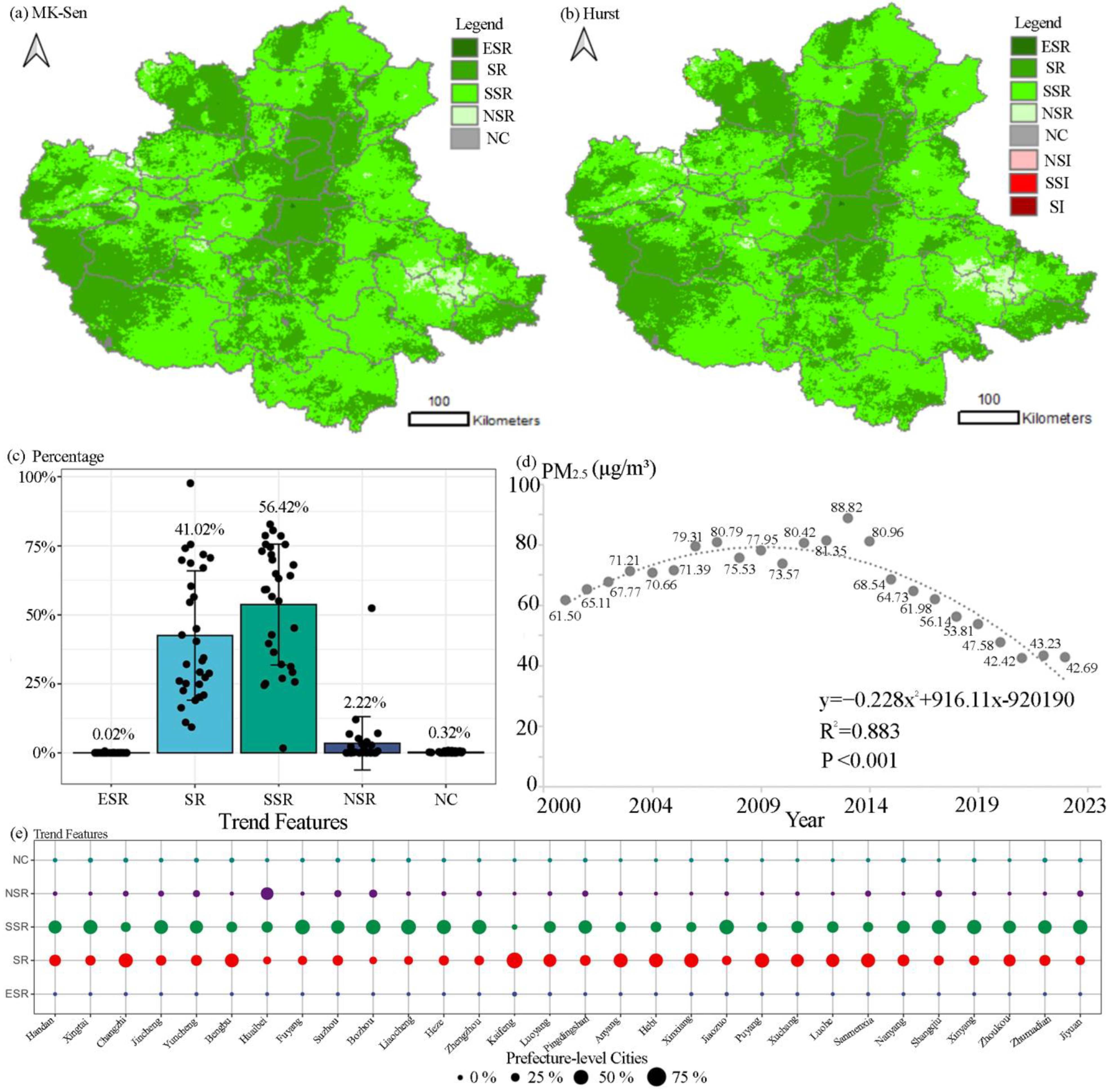
Figure 2 shows that from 2000 to 2023, the regions with highly significant reductions (HSRs) in PM2.5 were mainly concentrated in Zhengzhou, the core city of the CPUA, while the significant reductions (SR) were primarily distributed along the central development corridor and southwestern regions, forming a clear clustering pattern (Figure 2a). It was projected that 99.66% of the CPUA will maintain a continuously declining trend of PM2.5 concentrations, 0.33% will remain stable, and only 0.01% will display an upward trend in future 20 years (Figure 2b). The overall trend was dominated by significant reductions (SRs) and slightly significant reductions (SSRs), covering 0.118 million km2 (41.02% of the total area) and 0.162 million km2 (56.42%), respectively. In contrast, areas with no slight reduction (NSR) and no change (NC) accounted for 0.006 million km2 (2.22%) and 0.001 million km2 (0.32%), respectively (Figure 2c). The average PM2.5 concentration in the CPUA exhibited a distinct inverted U-shaped trajectory, increasing from 61.50 μg/m3 in 2020 to a peak of 88.82 μg/m3 in 2013, before declining to 42.69 μg/m3 in 2023 (R2 = 0.883, p < 0.001 ***, time series regression) (Figure 2d). At the prefecture-level city scale, only Huaibei was dominated by an NSR, while all other cities were dominated by SSRs and SRs, indicating that most cities in the CPUA were experiencing a continuous downward trend in PM2.5 concentrations (Figure 2e).

3.2. Regional Inequalities in the PM2.5 Concentration

Figure 3 shows that from 2000 to 2020, the overall Theil index of the CPUA decreased from 0.168 to 0.142, indicating a reduction in PM2.5 exposure inequality across the region. A significant decline was observed from 2011 to 2012, with the index dropping from 0.174 to 0.141. Within-group variation remained stable at approximately 0.043, while TBG decreased from 0.121 to 0.098, with a sharp drop from 0.130 to 0.099 during 2011–2012 (Figure 3a and Figure S3 and Tables S1–S3).
To further investigate air pollution exposure inequalities between urban and rural areas, the Theil indices were determined for these regions. In rural areas, the total Theil index decreased from 0.115 to 0.084. Between-group variation decreased significantly from 0.071 to 0.037, whereas TWG increased slightly from 0.044 to 0.047. Consequently, TWG’s contribution to overall inequality increased from 38% to 56%. Notably, in 2012, TWG surpassed TBG as the dominant factor causing inequality. In general, these phenomena indicated a growing disparity in rural PM2.5 exposure between cities. In urban areas, the total Theil index steadily increased from 0.096 to 0.208. A decomposition analysis of Theil index revealed a decline in TWG from 0.053 to 0.023, whereas there was an increase in TBG from 0.043 to 0.185. The contribution of TBG to the overall Theil index increased substantially, from 45% to 89%, indicating that inter-city disparity in PM2.5 exposure within urban areas continued to expand. In summary, the rural and overall inequalities of PM2.5 exposure have decreased with the growing disparity between cities becoming the primary driver of regional inequality in the CPUA (Figure 3b and Figure S5).

3.3. The Differences in the Driving Factors of Urban−Rural PM2.5 Exposure Inequality

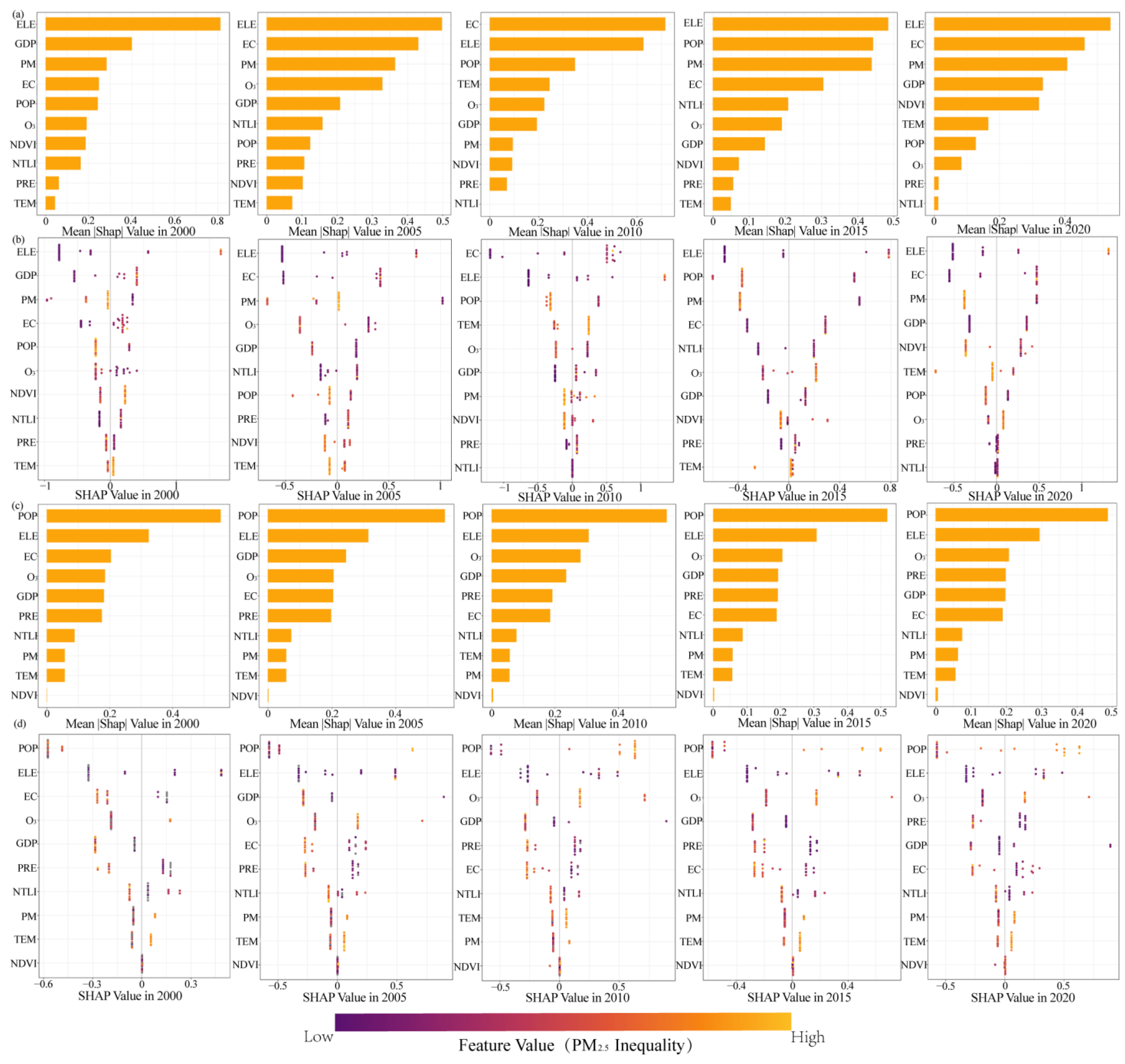
This study explored the inequalities in the drivers of PM2.5 exposure inequality across the CPUA as a whole and between urban and rural areas in 2000, 2005, 2010, 2015, and 2020. Figure 4a,b and Table S8 show that according to the average SHAP values for each of the five years, the factors with the greatest explanatory power for the inequality in PM2.5 exposure, from strongest to weakest, were as follows: elevation (0.593), electricity consumption (0.433), ground-level PM2.5 (0.318), population density (0.258), GDP (0.256), O3 concentration (0.204), NDVI (0.155), temperature (0.116), NTL (0.109), and precipitation (0.062). These results indicated that natural factors (i.e., elevation) had the strongest explanatory power for the inequality of overall PM2.5 exposure in the CPUA, while the impact of socio-economic covariates could not be ignored. In particular, electricity consumption should be given more attention (Figure 4a,b).
In rural areas of the CPUA, since most variables show significant differences in performance between the training set and the test set, most drivers had no explanatory power, with only elevation having notable SHAP values of 0.184, 0.392, 0.173, and 0.178 in 2000, 2005, 2015, and 2020, respectively, and temperature having a SHAP value of 0.221 in 2010. This indicated that consistent with the CPUA as a whole, natural factors (i.e., elevation) were the most significant explanatory factor for inequality in PM2.5 exposure in rural areas of the CPUA (Figure S1 and Table S8).
Figure 4c,d shows that in urban areas, population density consistently exhibited the strongest explanatory power throughout the study period, with mean values of 0.553, 0.555, 0.553, 0.520, and 0.482 in 2000, 2005, 2010, 2015, and 2020, respectively. Elevation was ranked as the second most influential factor, with average values of 0.324, 0.315, 0.306, 0.308, and 0.295 in 2000, 2005, 2010, 2015, and 2020, respectively. From the average SHAP values for the five years, the factors with the greatest explanatory power for inequality in PM2.5 exposure, from strongest to weakest, were the following: population density (0.534), elevation (0.310), O3 concentration (0.218), GDP (0.211), electricity consumption (0.195), precipitation (0.192), NTL (0.081), ground-level PM2.5 (0.059), temperature (0.057), and NDVI (0.004). Unlike the overall and rural areas of CPUA, the inequality of PM2.5 exposure in the urban areas of the CPUA was mainly influenced by factors such as population density, GDP, and electricity consumption. However, elevation still had a relatively strong influence. The O3 concentration should be managed in synergy with PM2.5 because of its strong explanatory power (Figure 4c,d).

3.4. Identifying Hotspots of PM2.5 Exposure Inequality

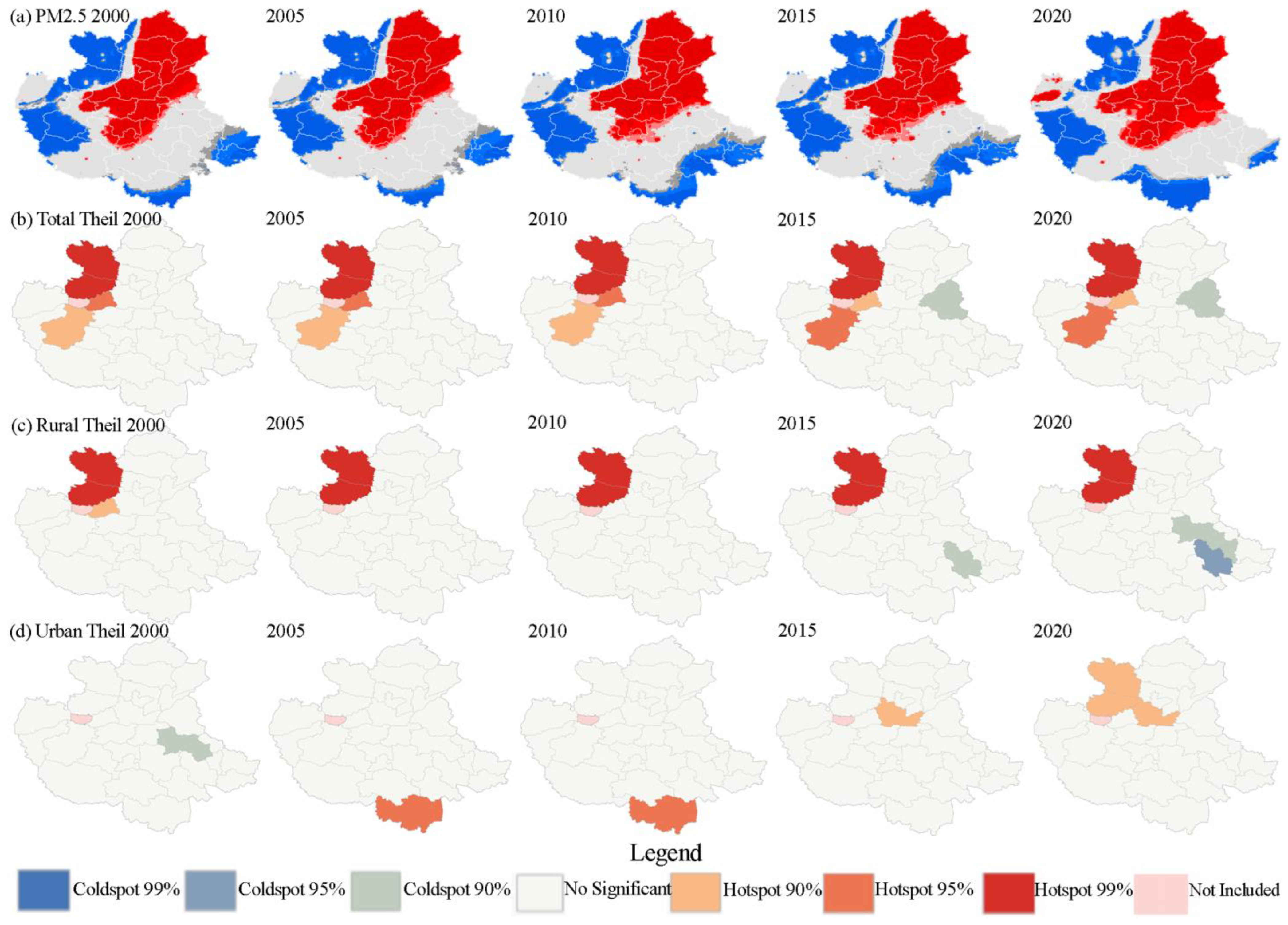
Figure 5 showed that from 2000 to 2020, the proportion of PM2.5-exposed coldspot areas decreased from 34.14% to 30.89%, while the proportion of hotspot areas increased from 31.08% to 36.60%. The coldspot areas were primarily located in the northwestern and southwestern regions of the CPUA. The hotspot areas were predominantly concentrated in the north-central part, with the remaining areas showing no significant changes. The hotspot areas in northeastern Zhoukou, Shangqiu, and Heze further expanded in size, and the hotspot areas in the north-central part of the CPUA spread further to the southeast. In Yuncheng in the northwestern part of the CPUA, there was a shrinkage of the coldspot area and the emergence of a hotspot area in 2020. At the same time, the coldspot areas in Fuyang, Xinyang, Bozhou, and Bengbu in the southwestern part of the CPUA declined further (Figure 5a and Figure S2). During the same periods, the overall hotspot areas based on the Theil index were largely concentrated in Changzhi, Jincheng, Luoyang, and Jiaozuo, reflecting an unequal spatial distribution of PM2.5 pollution exposure (Figure 5b). In rural areas, the Theil index hotspots were mainly observed in Changzhi, Jincheng, and Jiaozuo. Bozhou transitioned into a coldspot in 2015, and by 2020, Bozhou, Huaibei, and Shangqiu formed a coldspot cluster, signifying a spatial aggregation of regions with high equality in PM2.5 exposure in rural areas (Figure 5c). The Theil index values for urban areas did not have obvious spatial clustering characteristics, indicating that the characteristics of PM2.5 exposure inequality in the urban areas of the CPUA prefectural administrative divisions were more dispersed, which makes them unsuitable for collaborative management strategies (Figure 5d).

4. Discussion

4.1. Spatial and Temporal Change of PM2.5 Exposure in CPUA

During the study period, the PM2.5 concentrations in the CPUA initially exhibited an upward trend, followed by a marked decline after reaching an inflection point in 2013. This sustained decrease from 2013 to 2020 was closely associated with the implementation of the Air Pollution Prevention and Control Action Plan introduced by the Chinese government in 2013. The plan effectively curtailed PM2.5 levels by shutting down heavily polluting enterprises, enforcing strict pollution controls, and promoting environmentally friendly pollutant treatments [34,46]. Cities such as Anyang, Hebi, Xinxiang, Zhengzhou, Xuchang, Zhumadian, and Xinyang, situated within the central development corridor of the CPUA, were historically characterized by early industrialization and the dominance of heavy industry. Consequently, these regions experienced a significant reduction in PM2.5 levels post-2013 due to stringent policy measures. Notably, Zhengzhou, the central city of the CPUA, experienced a highly significant decline in PM2.5 concentrations. Zhenghou City implemented rigorous pollution control policies. However, it also faces persistent challenges from the urban heat island effect, which facilitates pollutant transport from surrounding areas to urban regions. Some studies have reported that PM2.5 concentrations are strongly correlated with the magnitude of the urban heat island effect. Furthermore, PM2.5 in the CPUA exhibits obvious spatial spillover and agglomeration effects, presenting significant challenges to the collaborative management of pollution between rural and urban areas, and within urban agglomerations [62,63]. Nevertheless, China’s air pollution control policy measures have resulted in continuous improvements in air quality within the CPUA [14].

4.2. Rural−Urban Differences in PM2.5 Exposure

The study revealed a declining trend in the overall inequality of PM2.5 pollution exposure across the CPUA, with a sharp reduction observed from 2011 to 2012. This significant improvement was largely attributed to the Chinese government’s 2011 Joint Air Pollutant Prevention and Control Policy, which promoted a coordinated approach to control regional air pollution. As PM2.5 exposure inequalities among cities narrowed, regional inequality in pollution exposure diminished, facilitating collaborative air pollutant management within urban agglomeration.
In rural areas, PM2.5 pollution exposure has steadily decreased from 2000 to 2004, stabilizing after 2005. This trend was aligned with the urbanization process in the CPUA, marked the fastest pace of urbanization, driven by the “New Rural Construction” policy and rural-to-urban migration [15,16]. These developments reduced variability in PM2.5 exposure in rural areas, improving public health and promoting equitable regional development [64].
Conversely, PM2.5 pollution exposure inequality in urban areas has steadily increased, a trend closely associated with the rapid pace of urban land development. This process has resulted in imbalanced regional development, leading to concentrated populations in heavily polluted urban and industrial zones [15]. This has increased urban residents’ exposure to air pollution. The failure of rapid urbanization to safeguard public health, ensure equitable development, and bridge economic inequalities among cities has perpetuated a vicious cycle [7]. Consequently, the inequalities in PM2.5 pollution exposure among urban areas have intensified, further exacerbating regional inequalities [65].

4.3. Differences in the Drivers of Inequality in PM2.5 Exposure Between Urban and Rural Areas

The RF-SHAP results revealed that elevation had the greatest explanatory power for both overall and rural PM2.5 exposure in the CPUA. It means that elevation was identified as the most influential factor contributing to the inequality of PM2.5 exposure in the CPUA. Elevation influences local wind patterns and terrain-induced airflow dynamics [66]. Low-lying areas are more prone to becoming pollutant convergence zones due to topographical constraints, which, when coupled with the urban heat island effect, can exacerbate the spatial disparity in PM2.5 exposure. Additionally, the transport of air pollutants is modulated by terrain-induced elevation differences. High-elevation areas are more likely to receive long-range transported pollutants from the upper atmosphere, while low-elevation regions primarily accumulate locally emitted pollutants [67,68].
Population density was identified as the strongest explanatory factor for regional inequality within the CPUA urban area, which suggests that the population density of residential areas may result in PM2.5 exposure inequalities [14]. In China’s urban agglomerations, vulnerable communities, such as impoverished neighborhoods and urban villages that often lack essential infrastructure (e.g., education and healthcare), typically have low population densities [22]. Conversely, areas with higher population densities tend to have more comprehensive infrastructure, making population density a crucial determinant in assessing inequalities in urban PM2.5 exposure [21,23]. Electricity consumption and GDP also significantly affected urban PM2.5 exposure inequalities. GDP exerted a dual impact during the initial stages of economic growth because it drove rapid regional development at the expense of environmental equality. Conversely, in the advanced stages of economic development, it fostered growth by encouraging the adoption of cleaner and more sustainable production practices [69]. It therefore alleviated PM2.5 exposure inequalities within the CPUA. Notably, the O3 concentration also had a substantial explanatory power for PM2.5 exposure inequalities, indicating an urgent need for integrated management strategies for both O3 and PM2.5 within the CPUA to effectively address environmental pollution inequalities [70].

4.4. Limitations of the Study and Future Outlook

The main limitation of this study was the spatial and temporal resolution of the data sources. The analysis relied on annual air pollution exposure data, and it was therefore difficult to incorporate higher temporal resolution data (e.g., daily or monthly PM2.5 levels) [34]. Additionally, the study’s temporal scope (2000–2023) and urban agglomeration scale necessitated the use of 1 × 1 km resolution raster data, which may have introduced underestimation or overestimation errors due to geospatial data uncertainties and potential spatial inaccuracies.
The second limitation was the exclusive use of the Theil index to calculate regional air exposure inequality at the municipal scale. While this approach is valid, previous studies employed alternative measures such as the Gini index, Hoffman index, and Atkinson index to assess regional development inequality [7,14]. The absence of these additional indices may have led to inaccuracies in the calculation of inequality. Furthermore, the study did not account for atmospheric dynamics and spatial diffusion effects, potentially overlooking cross-boundary interactions, such as the diffusion of air masses between Zhengzhou and Kaifeng in the CPUA [64], which could have affected air exposure inequality calculations at the prefecture-level scale.
Last, to maximize the capacity for capturing long-term trends in PM2.5 exposure inequality, we employed annual PM2.5 concentration data at a spatial resolution of 1 km. This choice was guided by the need to balance temporal coverage and spatial detail over an extended time series. Although higher temporal resolution data (e.g., monthly or daily) could potentially offer more detailed insights, previous studies have indicated that temporal variations in inequality at these finer scales are relatively minor.
To address these limitations, we propose several recommendations for future research. First, higher temporal resolution data, such as daily PM2.5 levels, could be used to focus on the number of polluted days rather than annual averages, mitigating the influence of extreme exposure days. Second, future studies should consider quantifying air inequality at the raster scale and analyzing regional air exposure inequalities across broader spatial scales. This approach would overcome the constraints of administrative boundaries, enabling a more precise assessment of inequalities within urban agglomerations. Finally, combining multiple inequality indices to measure air pollution exposure would help identify the most appropriate metric for urban agglomeration scales, fostering more effective collaborative air pollution management strategies.

5. Conclusions

This study used multi-source geospatial data to meticulously examine the trends in PM2.5 concentrations across the CPUA from 2000 to 2023 and then projected future patterns. This study answered three scientific questions:
(1) How have the spatial and temporal patterns of PM2.5 pollution evolved within representative urban agglomerations, and what insights can be derived from forecasting future trends and identifying pollution hotspots? A consistent downward trend in PM2.5 concentrations across the region was identified, with future trends expected to align with this trajectory. From 2000 to 2020, almost all of the CPUA exhibited a decreasing trend of PM2.5, which is in line with the Chinese government’s national strategy of “reducing the concentration of air pollutants”. Additionally, cold spots of PM2.5 exposure were concentrated in the northwestern and southwestern areas of the region, whereas hotspots were primarily located in the north-central areas.
(2) What are the dynamics of urban−rural PM2.5 exposure inequalities within urban agglomerations, and how have they changed over time? From 2000 to 2020, PM2.5 exposure inequalities decreased in both overall and rural areas but escalated in urban settings. Notably, Changzhi, Jincheng, Luoyang, and Jiaozuo were identified as the most significant hotspots of PM2.5 exposure inequality, underscoring the urgent need for integrated management strategies in these regions.
(3) How do natural, climate, and socio-economic drivers collectively influence urban−rural exposure inequalities, and what strategies can be adopted for effective mitigation? The overall PM2.5 exposure inequality and urban−rural inequalities were systematically analyzed, and the underlying drivers of spatial hotspots of exposure inequality were determined. Elevation emerged as a pivotal factor influencing exposure inequality in overall and rural areas, while population density was the main dominant factor in densely populated urban regions.
The main achievements of this study included accurately mapping the spatiotemporal dynamics of air pollution exposure within the CPUA; revealing regional inequalities in exposure inequality (at overall, urban, and rural scales); highlighting the critical need for intensified air pollution management in urban areas; and emphasizing the need to reduce inter-regional inequalities in exposure to achieve SDGs (SDG 3; SDG 10, and SDG 11). Furthermore, it quantified the driving forces of exposure inequality, providing localized, valuable evidence and actionable policy recommendations for the coordinated management of PM2.5 exposure inequalities. Ultimately, the findings of this study will advance sustainable development and foster social equity within the region.

Supplementary Materials

The following supporting information can be downloaded at: https://www.mdpi.com/article/10.3390/rs17172982/s1. Supplementary material to this article included the Supplementary Discussion, the Figures S1–S6, and the Tables S1–S8 [71,72,73,74,75,76,77,78].

Author Contributions

X.S.: Conceptualization, Methodology, Formal analysis, Visualization, Software, Writing—original draft. C.W.: Conceptualization, Formal analysis, Software, Writing—original draft. Y.J. (Yaqin Ji): Conceptualization, Writing—review and editing, Supervision, Funding acquisition, Project administration, Resources. Q.D.: Conceptualization, Methodology. Z.F.: Data Collection, Writing—review and editing. X.M.: Writing—review and editing. E.W.: Writing—review and editing. Y.J. (Yan Jiang): Writing—review and editing. W.F.: Writing—review and editing. All authors have read and agreed to the published version of the manuscript.

Funding

This research was funded by the Xinjiang Heavy Pollution Weather Emergency Control Capacity Building Project (Grant No. 2022-Local Research-1065), and the National Natural Science Foundation of China (Grant No. 32371863). And The APC was funded by the Xinjiang Heavy Pollution Weather Emergency Control Capacity Building Project (Grant No. 2022-Local Research-1065).

Data Availability Statement

Research Data can be found at Supplementary Material Table S1–S8, origin data can be found at Table 1, other data are available upon request from the corresponding author.

Acknowledgments

We also thank International Science Editing (http://www.internationalscienceediting.com) for editing this manuscript.

Conflicts of Interest

The authors declare that they have no known competing financial interests or personal relationships that could have appeared to influence the work reported in this paper.

References

  1. Yang, F.; Xu, Q.; Li, K.; Yuen, K.F.; Shi, W. The Inhibition Effect of Bank Credits on PM2.5 Concentrations: Spatial Evidence from High-Polluting Firms in China. Environ. Pollut. 2022, 308, 119639. [Google Scholar] [CrossRef]
  2. Tian, Y.; Ma, Y.; Xu, R.; Wu, Y.; Li, S.; Hu, Y.; Guo, Y. Landscape Fire PM2.5 and Hospital Admissions for Cause-Specific Cardiovascular Disease in Urban China. Nat. Commun. 2024, 15, 9604. [Google Scholar] [CrossRef]
  3. Wu, D.; Zheng, H.; Li, Q.; Wang, S.; Zhao, B.; Jin, L.; Lyu, R.; Li, S.; Liu, Y.; Chen, X.; et al. Achieving Health-Oriented Air Pollution Control Requires Integrating Unequal Toxicities of Industrial Particles. Nat. Commun. 2023, 14, 6491. [Google Scholar] [CrossRef]
  4. Yang, K.; Chen, D.-H.; Ding, X.; Li, J.; Zhang, Y.-Q.; Zhang, T.; Wang, Q.-Y.; Wang, J.-Q.; Cheng, Q.; Jiang, H.; et al. Different Roles of Primary and Secondary Sources in Reducing PM2.5: Insights from Molecular Markers in Pearl River Delta, South China. Atmos. Environ. 2023, 294, 119487. [Google Scholar] [CrossRef]
  5. Geng, G.; Zheng, Y.; Zhang, Q.; Xue, T.; Zhao, H.; Tong, D.; Zheng, B.; Li, M.; Liu, F.; Hong, C.; et al. Drivers of PM2.5 Air Pollution Deaths in China 2002–2017. Nat. Geosci. 2021, 14, 645–650. [Google Scholar] [CrossRef]
  6. Heft-Neal, S.; Burney, J.; Bendavid, E.; Burke, M. Robust Relationship between Air Quality and Infant Mortality in Africa. Nature 2018, 559, 254–258. [Google Scholar] [CrossRef]
  7. Yu, W.; Ye, T.; Chen, Z.; Xu, R.; Song, J.; Li, S.; Guo, Y. Global Analysis Reveals Region-Specific Air Pollution Exposure Inequalities. One Earth 2024, 7, 2063–2071. [Google Scholar] [CrossRef]
  8. Zhang, Q.; Zheng, Y.; Tong, D.; Shao, M.; Wang, S.; Zhang, Y.; Xu, X.; Wang, J.; He, H.; Liu, W.; et al. Drivers of Improved PM2.5 Air Quality in China from 2013 to 2017. Proc. Natl. Acad. Sci. USA 2019, 116, 24463–24469. [Google Scholar] [CrossRef]
  9. Zhou, Y.; Zhang, X.; Zhang, C.; Chen, B.; Gu, B. Mitigating Air Pollution Benefits Multiple Sustainable Development Goals in China. Environ. Pollut. 2024, 349, 123992. [Google Scholar] [CrossRef]
  10. Goforth, T.; Nock, D. Air Pollution Disparities and Equality Assessments of US National Decarbonization Strategies. Nat. Commun. 2022, 13, 7488. [Google Scholar] [CrossRef]
  11. Hou, L.; Dai, Q.; Song, C.; Liu, B.; Guo, F.; Dai, T.; Li, L.; Liu, B.; Bi, X.; Zhang, Y.; et al. Revealing Drivers of Haze Pollution by Explainable Machine Learning. Environ. Sci. Technol. Lett. 2022, 9, 112–119. [Google Scholar] [CrossRef]
  12. Yang, X.; Wang, L.; Ma, P.; He, Y.; Zhao, C.; Zhao, W. Urban and Suburban Decadal Variations in Air Pollution of Beijing and Its Meteorological Drivers. Environ. Int. 2023, 181, 108301. [Google Scholar] [CrossRef]
  13. Shu, L.; Wang, T.; Liu, J.; Chen, Z.; Wu, H.; Qu, Y.; Li, M.; Xie, M. Elucidating Drivers of Severe Wintertime Fine Particulate Matter Pollution Episodes in the Yangtze River Delta Region of Eastern China. Sci. Total Environ. 2024, 912, 169546. [Google Scholar] [CrossRef]
  14. Liu, Y.; Zhang, L.; Zang, Z.; Wang, Z.; Luo, Y.; Wang, H.; Jiao, L. Heterogeneity of Population Exposure to Particulate Matter Pollution and Its Socioeconomic Driving Mechanism in Shaanxi Province, China. Environ. Pollut. 2024, 363, 125274. [Google Scholar] [CrossRef]
  15. Niu, L.; Zhang, Z.; Liang, Y.; van Vliet, J. Spatiotemporal Patterns and Drivers of the Urban Air Pollution Island Effect for 2273 Cities in China. Environ. Int. 2024, 184, 108455. [Google Scholar] [CrossRef]
  16. Zhou, X.; Zhang, X.; Wang, Y.; Chen, W.; Li, Q. Spatio-Temporal Variations and Socio-Economic Drivers of Air Pollution: Evidence from 332 Chinese Prefecture-Level Cities. Atmos. Pollut. Res. 2023, 14, 101782. [Google Scholar] [CrossRef]
  17. Cushing, L.J.; Li, S.; Steiger, B.B.; Casey, J.A. Historical Red-Lining Is Associated with Fossil Fuel Power Plant Siting and Present-Day Inequalities in Air Pollutant Emissions. Nat. Energy 2023, 8, 52–61. [Google Scholar] [CrossRef]
  18. Zhao, J.; Tang, Y.; Zhu, X.; Zhu, J. National Environmental Monitoring and Local Enforcement Strategies. Nat. Cities 2025, 2, 58–69. [Google Scholar] [CrossRef]
  19. Zheng, Z.; Chen, L.; Sun, N.; Jin, Y.; Wang, Y. Pollution, Hazards, and Health Inequalities: A Longitudinal Exploration of the Impact of PM2.5 on Depression among Rural Older Adults with Different Incomes in China. Humanit. Soc. Sci. Commun. 2024, 11, 1682. [Google Scholar] [CrossRef]
  20. Deguen, S.; Zmirou-Navier, D. Social Inequalities Resulting from Health Risks Related to Ambient Air Quality—A European Review. Eur. J. Public Health 2010, 20, 27–35. [Google Scholar] [CrossRef]
  21. Liao, L.; Du, M.; Chen, Z. Environmental Pollution and Socioeconomic Health Inequality: Evidence from China. Sustain. Cities Soc. 2023, 95, 104579. [Google Scholar] [CrossRef]
  22. Liu, M.; Wang, Y.; Liu, R.; Ding, C.; Zhou, G.; Han, L. How Magnitude of PM2.5 Exposure Disparities Have Evolved across Chinese Urban-Rural Population during 2010–2019. J. Clean. Prod. 2023, 382, 135333. [Google Scholar] [CrossRef]
  23. Nunez, Y.; Benavides, J.; Shearston, J.A.; Krieger, E.M.; Daouda, M.; Henneman, L.R.F.; McDuffie, E.E.; Goldsmith, J.; Casey, J.A.; Kioumourtzoglou, M.-A. An Environmental Justice Analysis of Air Pollution Emissions in the United States from 1970 to 2010. Nat. Commun. 2024, 15, 268. [Google Scholar] [CrossRef]
  24. Testi, I.; Wang, A.; Paul, S.; Mora, S.; Walker, E.; Nyhan, M.; Duarte, F.; Santi, P.; Ratti, C. Big Mobility Data Reveals Hyperlocal Air Pollution Exposure Disparities in the Bronx, New York. Nat. Cities 2024, 1, 512–521. [Google Scholar] [CrossRef]
  25. Ban, J.; Lu, K.; Wang, Q.; Li, T. Climate Change Will Amplify the Inequitable Exposure to Compound Heatwave and Ozone Pollution. One Earth 2022, 5, 677–686. [Google Scholar] [CrossRef]
  26. Li, Y.; Li, B.; Liao, H.; Zhou, B.-B.; Wei, J.; Wang, Y.; Zang, Y.; Yang, Y.; Liu, R.; Wang, X. Changes in PM2.5-Related Health Burden in China’s Poverty and Non-Poverty Areas during 2000–2020: A Health Inequality Perspective. Sci. Total Environ. 2023, 861, 160517. [Google Scholar] [CrossRef]
  27. Smith, G.S.; Anjum, E.; Francis, C.; Deanes, L.; Acey, C. Climate Change, Environmental Disasters, and Health Inequities: The Underlying Role of Structural Inequalities. Curr. Environ. Health Rep. 2022, 9, 80–89. [Google Scholar] [CrossRef]
  28. Kang, J.; Zhang, B.; Zhang, J.; Dang, A. Quantifying the Effects of Different Containment Policies on Urban NO2 Decline: Evidence from Remote Sensing and Ground-Station Data. Remote Sens. 2023, 15, 1068. [Google Scholar] [CrossRef]
  29. He, T.; Song, H. A Novel Approach to Assess the Urban Land-Use Efficiency of 767 Resource-Based Cities in China. Ecol. Indic. 2023, 151, 110298. [Google Scholar] [CrossRef]
  30. Martins, F.P.; Closs, J.G.; Waked, D.; Saldiva, P.H.N.; Veras, M.M. Positive Impacts of Air Pollution Reduction on SDG 3 Targets in Urban Environment. In Integrated Science for Sustainable Development Goal 3: Universal Good Health and Well-Being; Rezaei, N., Ed.; Springer Nature Switzerland: Cham, Switzerland, 2024; pp. 269–292. ISBN 978-3-031-64292-0. [Google Scholar]
  31. Wang, C.; Liu, S.; Feng, T.; Liu, Y.; Liu, Y.; Hu, Z.; Yang, L.; Niu, Q.; Mao, X. Is the Assessment Approach of Sustainable Development Goal 11.3.1 Justified? Evidence from the Drivers of Future Urban Land Use Efficiency. J. Clean. Prod. 2024, 444, 141147. [Google Scholar] [CrossRef]
  32. Zhu, J.; Zhai, Y.; Feng, S.; Tan, Y.; Wei, W. Trade-Offs and Synergies among Air-Pollution-Related SDGs as Well as Interactions between Air-Pollution-Related SDGs and Other SDGs. J. Clean. Prod. 2022, 331, 129890. [Google Scholar] [CrossRef]
  33. Mu, W.; Zhu, X.; Ma, W.; Han, Y.; Huang, H.; Huang, X. Impact Assessment of Urbanization on Vegetation Net Primary Productivity: A Case Study of the Core Development Area in Central Plains Urban Agglomeration, China. Environ. Res. 2023, 229, 115995. [Google Scholar] [CrossRef]
  34. Wei, J.; Li, Z.; Lyapustin, A.; Sun, L.; Peng, Y.; Xue, W.; Su, T.; Cribb, M. Reconstructing 1-Km-Resolution High-Quality PM2.5 Data Records from 2000 to 2018 in China: Spatiotemporal Variations and Policy Implications. Remote Sens. Environ. 2021, 252, 112136. [Google Scholar] [CrossRef]
  35. Wei, J.; Li, Z.; Cribb, M.; Huang, W.; Xue, W.; Sun, L.; Guo, J.; Peng, Y.; Li, J.; Lyapustin, A.; et al. Improved 1&thinsp;Km Resolution PM2.5 Estimates across China Using Enhanced Space–Time Extremely Randomized Trees. Atmos. Chem. Phys. 2020, 20, 3273–3289. [Google Scholar] [CrossRef]
  36. Zhao, M.; Cheng, C.; Zhou, Y.; Li, X.; Shen, S.; Song, C. A Global Dataset of Annual Urban Extents (1992–2020) from Harmonized Nighttime Lights. Earth Syst. Sci. Data 2022, 14, 517–534. [Google Scholar] [CrossRef]
  37. Yang, J.; Dong, J.; Xiao, X.; Dai, J.; Wu, C.; Xia, J.; Zhao, G.; Zhao, M.; Li, Z.; Zhang, Y.; et al. Divergent Shifts in Peak Photosynthesis Timing of Temperate and Alpine Grasslands in China. Remote Sens. Environ. 2019, 233, 111395. [Google Scholar] [CrossRef]
  38. Danielson, J.J.; Gesch, D.B. Global Multi-resolution Terrain Elevation Data 2010 (GMTED2010); USGS Open-File Report 2011-1073; U.S. Geological Survey: Reston, VA, USA, 2011.
  39. Peng, S. 1-Km Monthly Precipitation Dataset for CHINA (1901–2024); National Tibetan Plateau/Third Pole Environment Data Center: Beijing, China, 2020. [Google Scholar] [CrossRef]
  40. Peng, S. 1-km Monthly Mean Temperature Dataset for China (1901-2024); National Tibetan Plateau/Third Pole Environment Data Center: Beijing, China, 2019. [Google Scholar]
  41. Chen, J.; Gao, M.; Cheng, S.; Hou, W.; Song, M.; Liu, X.; Liu, Y. Global 1 Km × 1 Km Gridded Revised Real Gross Domestic Product and Electricity Consumption during 1992–2019 Based on Calibrated Nighttime Light Data. Sci. Data 2022, 9, 202. [Google Scholar] [CrossRef]
  42. Wei, J.; Li, Z.; Li, K.; Dickerson, R.R.; Pinker, R.T.; Wang, J.; Liu, X.; Sun, L.; Xue, W.; Cribb, M. Full-Coverage Mapping and Spatiotemporal Variations of Ground-Level Ozone (O3) Pollution from 2013 to 2020 across China. Remote Sens. Environ. 2022, 270, 112775. [Google Scholar] [CrossRef]
  43. Chen, Z.; Yu, B.; Yang, C.; Zhou, Y.; Yao, S.; Qian, X.; Wang, C.; Wu, B.; Wu, J. An Extended Time Series (2000–2018) of Global NPP-VIIRS-like Nighttime Light Data from a Cross-Sensor Calibration. Earth Syst. Sci. Data 2021, 13, 889–906. [Google Scholar] [CrossRef]
  44. Bhaduri, B.; Bright, E.; Coleman, P.; Dobson, J. LandScan. Geoinformatics 2002, 5, 34–37. [Google Scholar]
  45. Liu, H.; Jiang, D.; Yang, X.; Luo, C. Spatialization Approach to 1 Km Grid GDP Supported by Remote Sensing. Geo-Inf. Sci. 2005, 7, 120–123. [Google Scholar]
  46. Li, K.; Li, C.; Hu, Y.; Xiong, Z.; Wang, Y. Quantitative Estimation of the PM2.5 Removal Capacity and Influencing Factors of Urban Green Infrastructure. Sci. Total Environ. 2023, 867, 161476. [Google Scholar] [CrossRef]
  47. Wang, A.; Zhang, M.; Chen, E.; Zhang, C.; Han, Y. Impact of Seasonal Global Land Surface Temperature (LST) Change on Gross Primary Production (GPP) in the Early 21st Century. Sustain. Cities Soc. 2024, 110, 105572. [Google Scholar] [CrossRef]
  48. Kendall, M.G. Rank Correlation Methods; Charles Griffin: London, UK, 1948. [Google Scholar]
  49. Mann, H.B. Nonparametric Tests Against Trend. Econometrica 1945, 13, 245–259. [Google Scholar] [CrossRef]
  50. Sen, P.K. Estimates of the Regression Coefficient Based on Kendall’s Tau. J. Am. Stat. Assoc. 1968, 63, 1379–1389. [Google Scholar] [CrossRef]
  51. Hurst, H.E. Long-Term Storage Capacity of Reservoirs. Trans. Am. Soc. Civ. Eng. 1951, 116, 770–799. [Google Scholar] [CrossRef]
  52. Conceicao, P.; Ferreira, P. The Young Person’s Guide to the Theil Index: Suggesting Intuitive Interpretations and Exploring Analytical Applications; University of Texas at Austin: Austin, TX, USA, 2000. [Google Scholar]
  53. Zhao, T.; Zhang, X.; Liu, W.; Wang, J.; Li, Z.; Liu, L. Increase in per Capita Cropland Imbalance across Countries from 1985 to 2022: A Threat to Achieving Sustainable Development Goals. Geogr. Sustain. 2025, 6, 100239. [Google Scholar] [CrossRef]
  54. Breiman, L. Random Forests. Mach. Learn. 2001, 45, 5–32. [Google Scholar] [CrossRef]
  55. Yang, Y.; Shi, M.; Liu, B.; Yi, Y.; Wang, J.; Zhao, H. Contribution of Ecological Restoration Projects to Long-Term Changes in PM2.5. Ecol. Indic. 2024, 159, 111630. [Google Scholar] [CrossRef]
  56. Chen, T.; Guestrin, C. XGBoost: A Scalable Tree Boosting System. In Proceedings of the 22nd ACM SIGKDD International Conference on Knowledge Discovery and Data Mining, San Francisco, CA, USA, 13 August 2016; ACM: New York, NY, USA; pp. 785–794. [Google Scholar]
  57. Van den Broeck, G.; Lykov, A.; Schleich, M.; Suciu, D. On the Tractability of SHAP Explanations. J. Artif. Intell. Res. 2022, 74, 851–886. [Google Scholar] [CrossRef]
  58. Chen, X.; Ma, W.; Zheng, F.; Wang, Z.; Hua, C.; Li, Y.; Wu, J.; Li, B.; Jiang, J.; Yan, C.; et al. Identifying Driving Factors of Atmospheric N2O5 with Machine Learning. Environ. Sci. Technol. 2024, 58, 11568–11577. [Google Scholar] [CrossRef]
  59. Shao, T.; Wang, P.; Yu, W.; Gao, Y.; Zhu, S.; Zhang, Y.; Hu, D.; Zhang, B.; Zhang, H. Drivers of Alleviated PM2.5 and O3 Concentrations in China from 2013 to 2020. Resour. Conserv. Recycl. 2023, 197, 107110. [Google Scholar] [CrossRef]
  60. Zhang, Z.; Xu, B.; Xu, W.; Wang, F.; Gao, J.; Li, Y.; Li, M.; Feng, Y.; Shi, G. Machine Learning Combined with the PMF Model Reveal the Synergistic Effects of Sources and Meteorological Factors on PM2.5 Pollution. Environ. Res. 2022, 212, 113322. [Google Scholar] [CrossRef]
  61. Manepalli, U.; Bham, G.H.; Kandada, S. Evaluation of Hotspots Identification Using Kernel Density Estimation (K) and Getis-Ord (Gi*) on I-630. In Proceedings of the 3rd International Conference on Road Safety and Simulation; National Academy of Sciences Indianapolis Indiana, Indianapolis, IN, USA, 14–16 September 2011; Volume 21, pp. 14–16. [Google Scholar]
  62. Yang, F.; Yu, J.; Zhang, C.; Li, L.; Lei, Y.; Wu, S.; Wang, Y.; Zhang, X. Spatio-Temporal Differentiation Characteristics and the Influencing Factors of PM2.5 Emissions from Coal Consumption in Central Plains Urban Agglomeration. Sci. Total Environ. 2024, 945, 173778. [Google Scholar] [CrossRef]
  63. Zhang, P.; Zhang, J.; Liu, Z.; Liu, Y.; Chen, Z. Relationship between Land Surface Temperature and Air Quality in Urban and Suburban Areas: Dynamic Changes and Interaction Effects. Sustain. Cities Soc. 2025, 118, 106043. [Google Scholar] [CrossRef]
  64. Luo, H.; Li, L.; Lei, Y.; Wu, S.; Yan, D.; Fu, X.; Luo, X.; Wu, L. Decoupling Analysis between Economic Growth and Resources Environment in Central Plains Urban Agglomeration. Sci. Total Environ. 2021, 752, 142284. [Google Scholar] [CrossRef]
  65. Li, W.; Yi, P.; Yu, H.; Lin, W.; Wu, X. Assessment on Sustainable Development of Three Major Urban Agglomerations in China Based on Sustainability-Differentiation-Combined Weighting Method. Sustain. Dev. 2023, 31, 2678–2693. [Google Scholar] [CrossRef]
  66. Jaén, C.; Titos, G.; Castillo, S.; Casans, A.; Rejano, F.; Cazorla, A.; Herrero, J.; Alados-Arboledas, L.; Grimalt, J.O.; van Drooge, B.L. Diurnal Source Apportionment of Organic and Inorganic Atmospheric Particulate Matter at a High-Altitude Mountain Site under Summer Conditions (Sierra Nevada; Spain). Sci. Total Environ. 2023, 905, 167178. [Google Scholar] [CrossRef]
  67. Gao, Z.; Wang, F.; Du, W.; Wang, S.; Sun, Y.; Yang, W.; Wang, X.; Han, B.; Bai, Z. Elucidating Particle Number Concentrations and Unveiling Source Mechanisms at a Prominent National Background Site on the Northeastern Qinghai-Tibetan Plateau. Sci. Total Environ. 2025, 969, 178928. [Google Scholar] [CrossRef]
  68. Luo, Q.; Liu, W.; Wang, C. Air Pollution Transmission Networks in China’s Urban Agglomerations: Drivers and Vulnerabilities. Cities 2025, 166, 106237. [Google Scholar] [CrossRef]
  69. Zhang, Y.; Shuai, C.; Bian, J.; Chen, X.; Wu, Y.; Shen, L. Socioeconomic Factors of PM2.5 Concentrations in 152 Chinese Cities: Decomposition Analysis Using LMDI. J. Clean. Prod. 2019, 218, 96–107. [Google Scholar] [CrossRef]
  70. Zhao, K.; Yuan, Z.; Wu, Y.; Huang, J.; Yang, F.; Zhang, X.; Huang, D.; Jiang, R. Identification of Synergistic Control for Ozone and PM2.5 Pollution during a Large-Scale Emission Reduction in China. Atmos. Res. 2023, 295, 107025. [Google Scholar] [CrossRef]
  71. Sharifi, A.; Allam, Z.; Bibri, S.E.; Khavarian-Garmsir, A.R. Smart Cities and Sustainable Development Goals (SDGs): A Systematic Literature Review of Co-Benefits and Trade-Offs. Cities 2024, 146, 104659. [Google Scholar] [CrossRef]
  72. Xu, X.; Zhang, Z.; Long, T.; Sun, S.; Gao, J. Mega-City Region Sustainability Assessment and Obstacles Identification with GIS–Entropy–TOPSIS Model: A Case in Yangtze River Delta Urban Agglomeration, China. J. Clean. Prod. 2021, 294, 126147. [Google Scholar] [CrossRef]
  73. Ji, X.; Chen, B. Assessing the Energy-Saving Effect of Urbanization in China Based on Stochastic Impacts by Regression on Population, Affluence and Technology (STIRPAT) Model. J. Clean. Prod. 2017, 163, S306–S314. [Google Scholar] [CrossRef]
  74. Zhang, Q.; Cao, Z.; Liu, Y. Assessing Rural Revitalization Potential through Rural Transformation Degree and Sustainability: A Quantitative Study of 460 Case Villages in Lingbao, China. Habitat Int. 2024, 153, 103194. [Google Scholar] [CrossRef]
  75. Liu, J.; Xue, L.; Huang, X.; Wang, Z.; Lou, S.; Ding, A. Intensified Haze Formation and Meteorological Feedback by Complex Terrain in the North China Plain Region. Atmospheric Ocean. Sci. Lett. 2023, 16, 100273. [Google Scholar] [CrossRef]
  76. Schmidt-Traub, G.; Kroll, C.; Teksoz, K.; Durand-Delacre, D.; Sachs, J.D. National Baselines for the Sustainable Development Goals Assessed in the SDG Index and Dashboards. Nat. Geosci. 2017, 10, 547–555. [Google Scholar] [CrossRef]
  77. Wang, C.; Liu, S.; Zhou, S.; Zhou, J.; Jiang, S.; Zhang, Y.; Feng, T.; Zhang, H.; Zhao, Y.; Lai, Z.; et al. Spatial-Temporal Patterns of Urban Expansion by Land Use/Land Cover Transfer in China. Ecol. Indic. 2023, 155, 111009. [Google Scholar] [CrossRef]
  78. Xu, Z.; Chau, S.N.; Chen, X.; Zhang, J.; Li, Y.; Dietz, T.; Wang, J.; Winkler, J.A.; Fan, F.; Huang, B.; et al. Assessing Progress towards Sustainable Development over Space and Time. Nature 2020, 577, 74–78. [Google Scholar] [CrossRef]
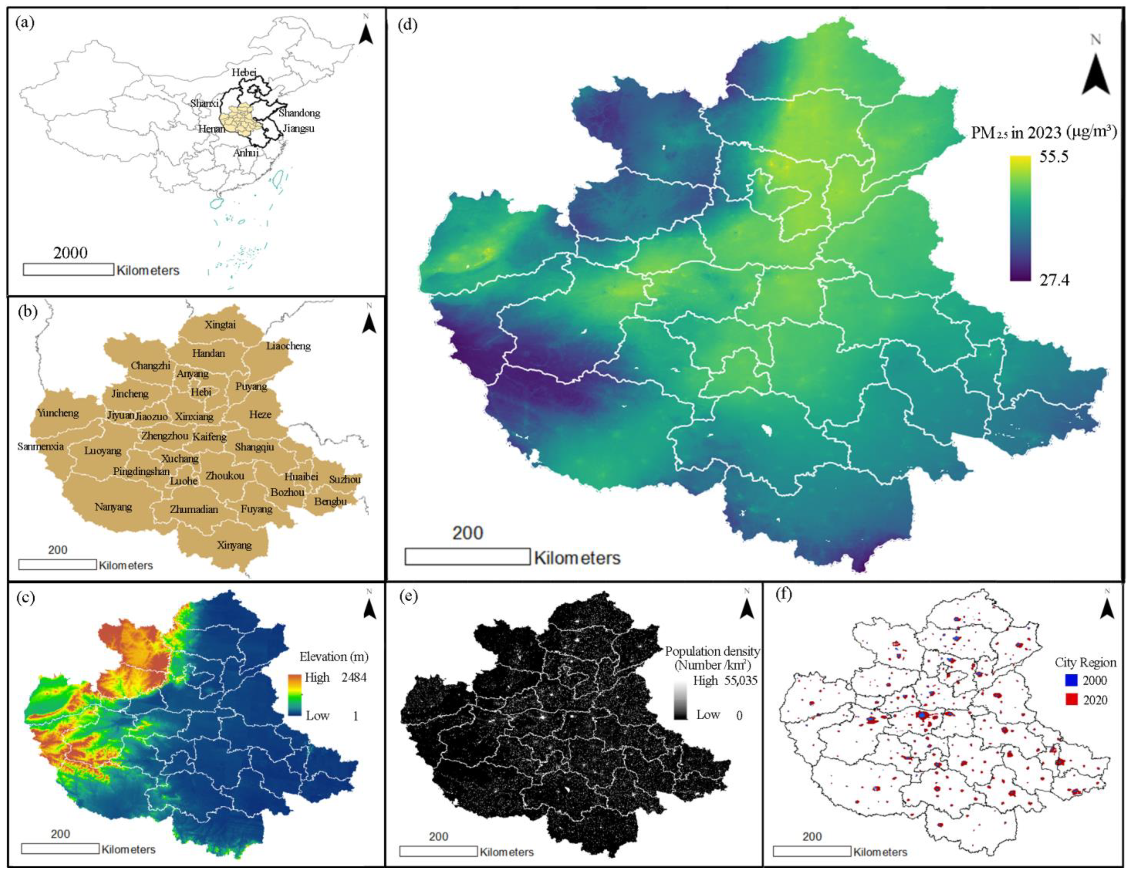
Figure 1. Map of the study area. (a). Geographic location of the Central Plains Urban Agglomeration (CPUA) in China. (b). Spatial distribution of the 30 prefecture-level cities within the CPUA. (c). Elevation of the CPUA, derived from a digital elevation model (DEM). (d). The PM2.5 concentration across the CPUA in 2023, mapped at a resolution of 1 × 1 km. (e). A population density map of the CPUA in 2020. (f). Urban expansion in the CPUA between 2000 and 2020, with blue representing areas built prior to 2000 and red indicating newly developed areas after 2000.
Remotesensing 17 02982 g001
Figure 2. Trends in PM2.5 intensity and spatiotemporal evolution across the Central Plains Urban Agglomeration (CPUA). (a). Sen-MK test results showing the PM2.5 concentration trends. (b). Future PM2.5 concentration trends derived from the Hurst index. (c). Percentage distribution of the five PM2.5 trend categories across cities. (d). Interannual variation in the average PM2.5 concentration. (e). Spatial distribution of PM2.5 concentration trends across 30 prefectural-level cities.
Remotesensing 17 02982 g002
Figure 3. Spatial and temporal characteristics of PM2.5 inequality. (a). Theil indices for the whole region, rural, and urban areas. (b). Temporal distributions of the Theil indices from 2000 to 2020.
Remotesensing 17 02982 g003
Figure 4. The SHapley Additive exPlanations (SHAP) values in 2000, 2005, 2010, 2015, and 2020. (a). Average SHAP values for overall PM2.5 exposure inequality within the CPUA. (b). A bee swarm plot of the individual SHAP values for overall PM2.5 exposure inequality within the CPUA. The y-axis stands for the different driving factors. (c). Average SHAP values for PM2.5 exposure inequality in urban areas within the CPUA. (d). A bee swarm plot of the individual SHAP values for PM2.5 exposure inequality in urban areas within the CPUA. The y-axis stands for the different driving factors. (Note vegetation cover (NDVI), elevation (ELE), precipitation (PRE), temperature (TEM), PM2.5 (PM), electricity consumption (EC), ozone concentration (O3), nighttime lighting (NTL), population density (POP), and gross domestic production (GDP)).
Remotesensing 17 02982 g004
Figure 5. Spatial hotspot−coldspot distribution of PM2.5 concentration and inequality in the Central Plains Urban Agglomeration (CPUA) every five years from 2000 to 2020. (a). Spatial hotspot−coldspot distribution of PM2.5 concentration at the grid scale (1 × 1 km), where light orange, orange-red, and red represent hotspots with confidence levels of 90%, 95%, and 99%, respectively. Grey, light blue, and dark blue represent coldspots with confidence levels of 90%, 95%, and 99%, respectively; white represents areas without significant change. (b). Spatial hotspot−coldspot distribution of the overall PM2.5 Theil index at the prefecture-level city scale. (c). Spatial hotspot−coldspot distribution of the PM2.5 Theil index in rural areas at the prefecture-level city scale. (d). Spatial hotspot−coldspot distribution of the PM2.5 Theil index in urban areas at the prefecture-level city scale.
Remotesensing 17 02982 g005
Table 1. Indicators, source, and classification of all the data used in this study (All data accessed on 25 August 2025).
DimensionIndicatorSpatial ResolutionSourceReference
PollutionPM2.5 (PM)1000 mhttps://zenodo.org/records/13340222[34,35]
UrbanUrban Built Area1000 mhttps://doi.org/10.6084/m9.figshare.16602224.v1[36]
NaturalNormalized Difference Vegetation Index (NDVI)1000 mhttps://www.earthdata.nasa.gov/[37]
Elevation (ELE)1000 mhttps://search.earthdata.nasa.gov/[38]
ClimatePrecipitation (PRE)1000 mhttps://data.tpdc.ac.cn/zh-hans/data[39]
Temperature (TEM)1000 mhttps://data.tpdc.ac.cn/zh-hans/data[40]
DischargeElectricity consumption (EC)1000 mhttps://doi.org/10.6084/m9.figshare.17004523.v1[41]
Ozone Concentration(O3)1000 mhttp://geodata.nnu.edu.cn/data[42]
Social-EconomicNighttime light (NTL)1000 mhttp://geodata.nnu.edu.cn/[43]
Population density (POP)1000 mhttps://www.eastview.com/resources/e-collections/landscan/[44]
Gross Domestic Product (GDP)1000 mhttps://www.resdc.cn/doi/doi.aspx?DOIid = 33[45]
Table 2. Eight levels defining the temporal variation of PM2.5 intensity.
βZTrend TypeTrend Features
>0|Z| > 2.584Extremely significant increase (ESI)
1.96 < |Z| ≤ 2.583Significant increase (SI)
1.65 < |Z| ≤ 1.962Slightly significant increase (SSI)
|Z| ≤ 1.651No significant increase (NSI)
0Z = 00No change (NC)
<0|Z| ≤ 1.65−1No significant reduction (NSR)
1.65 < |Z| ≤ 1.96−2Slightly significant reduction (SSR)
1.96 < |Z| ≤ 2.58−3Significant reduction (SR)
|Z| > 2.58−4Extremely significant reduction (ESR)
Disclaimer/Publisher’s Note: The statements, opinions and data contained in all publications are solely those of the individual author(s) and contributor(s) and not of MDPI and/or the editor(s). MDPI and/or the editor(s) disclaim responsibility for any injury to people or property resulting from any ideas, methods, instructions or products referred to in the content.