Article

A GRU-Enhanced Kolmogorov–Arnold Network Model for Sea Surface Temperature Prediction Derived from Satellite Altimetry Product in South China Sea

1
School of Transportation Engineering, East China Jiaotong University, Nanchang 330013, China
2
Jiangxi Provincial Key Laboratory of Comprehensive Stereoscopic Traffic Information Perception and Fusion, East China Jiaotong University, Nanchang 330013, China
*
Author to whom correspondence should be addressed.
Remote Sens. 2025, 17(16), 2916; https://doi.org/10.3390/rs17162916
Submission received: 2 July 2025 / Revised: 9 August 2025 / Accepted: 20 August 2025 / Published: 21 August 2025

Abstract

High-precision Sea Surface Temperature (SST) prediction is critical for understanding ocean–atmosphere interactions and climate anomaly monitoring. We propose GRU_EKAN, a novel hybrid model where Gated Recurrent Units (GRUs) capture temporal dependencies and the Enhanced Kolmogorov–Arnold Network (EKAN) models complex feature interactions between SST and multivariate ocean predictors. This study integrates GRU with EKAN, using B-spline-parameterized activation functions to model high-dimensional nonlinear relationships between multiple ocean variables (including sea water potential temperature at the sea floor, ocean mixed layer thickness defined by sigma theta, sea water salinity, current velocities, and sea surface height) and SST. L2 regularization addresses multicollinearity among predictors. Experiments were conducted at 25 South China Sea sites using 2011–2021 CMEMS data. The results show that GRU_EKAN achieves a superior mean R2 of 0.85, outperforming LSTM_EKAN, GRU, and LSTM by 5%, 25%, and 23%, respectively. Its average RMSE (0.90 °C), MAE (0.76 °C), and MSE (0.80 °C2) represent reductions of 31.3%, 27.0%, and 53.2% compared to GRU. The model also exhibits exceptional stability and minimal Weighted Quality Evaluation Index (WQE) fluctuation. During the 2019–2020 temperature anomaly events, GRU_EKAN predictions aligned closest with observations and captured abrupt trend shifts earliest. This model provides a robust tool for high-precision SST forecasting in the South China Sea, supporting marine heatwave warnings.

Graphical Abstract

1. Introduction

Given the close interconnection between the ocean and the atmosphere, there is a continuous exchange of heat, momentum, and mass across their interface [1]. SST is a key component in this dynamic interaction and facilitates heat transfer between the two systems [2]. Therefore, accurately predicting SST variations is essential for understanding the complex dynamic mechanisms in both the ocean and the atmosphere [3].
Earlier marine temperature studies often integrated temperature data with ocean circulation models. These models were constructed by formulating dynamic and thermodynamic equations and solving PDEs (Partial Differential Equations) to make predictions [4,5,6,7]. However, these models had certain limitations. Their parametrization schemes were not entirely perfect. Errors in initial/boundary conditions could accumulate easily. Quantifying climate patterns and sea level trends was challenging. Moreover, their high computational cost and low efficiency restricted their real-time use and applications. Data-driven methods, particularly machine learning, which learn patterns directly from observational data, have shown great potential [8,9,10,11,12].
Driven by advances in machine learning and deep learning, significant progress has been achieved in SST prediction globally. International research has successfully deployed sophisticated architectures to capture SST’s complex spatiotemporal nature. Recurrent Neural Networks (RNNs), particularly Long Short-Term Memory (LSTM) and Gated Recurrent Units (GRUs), have proven effective in modeling temporal dependencies for global and regional forecasts, as demonstrated by Ham et al.’s LSTM model for multi-year ENSO (El Niño–Southern Oscillation) predictions [13] and Wanigasekara et al.’s Fast MEEMD–ConvLSTM (Multidimensional Ensemble Empirical Mode Decomposition–Convolutional Long Short-Term Memory) model for predicting sea surface temperature in the Indian Ocean [14]. While Transformers leverage self-attention for long-range dependencies, this is exemplified by the work of Dai et al. on long-term global sea surface temperature prediction using a Temporal Embedding Transformer with Attention Distilling and Partial Stacked Connection [15]. Critically, integrating physical knowledge has emerged as a key frontier to enhance robustness and interpretability. Physics-Informed Neural Networks (PINNs) have been effectively applied to embed ocean thermodynamics into SST prediction, as demonstrated by Meng et al. in their study on physical knowledge-enhanced deep neural networks [16]. Similarly, architectures like STPDE-Net (Space-Time Partial Differential Equation) explicitly encode partial differential equation structures to enhance prediction accuracy [17]. In parallel, efforts within China have adapted these deep learning paradigms to regional seas, yielding tailored solutions. For instance, hybrid models like RC-LSTM (Regional Convolutional Long Short-Term Memory network) have improved short-term forecasts of sea surface temperature (SST) in China’s coastal waters [18]. The Global Cross-Scale Spatiotemporal Attention Deep Neural Network (GCSA-DNN) model, proposed by Li et al., has demonstrated significant improvements in SST predictions for Chinese coastal waters [19]. Additionally, Transformers show promise for seasonal prediction in the Bohai Sea [20].
Despite these substantial advancements, a critical limitation persistently constrains the accuracy and robustness of current ML/DL SST prediction models, both internationally and domestically, particularly in dynamically complex regions like the SCS: a predominant reliance on historical SST as the primary or sole input variable. While competent performance is achievable with single-variable inputs in some contexts [20,21], this approach fundamentally limits predictive potential in environments characterized by complex, multi-factor interactions like the SCS. Furthermore, attempts to incorporate these valuable multiple predictors introduce the inherent challenge of multicollinearity—high correlations among input variables [22,23]. If not explicitly mitigated, multicollinearity degrades model stability, inflates parameter variance, and ultimately reduces prediction accuracy, counteracting the anticipated benefits of richer input data.
To overcome these intertwined limitations—the underutilization of multivariate information and the unaddressed challenge of multicollinearity—and unlock enhanced SST forecasting capability for the SCS, this study introduces a novel hybrid deep learning architecture, GRU_EKAN, and a comprehensive modeling strategy. First, we propose the GRU_EKAN model, uniquely integrating a GRU network, which is adept at learning long-term temporal dependencies within SST sequences, with an Enhanced Kolmogorov–Arnold Network (EKAN). Crucially, EKAN replaces the standard Multi-Layer Perceptron (MLP) at the GRU’s output stage. Leveraging the Kolmogorov–Arnold representation theorem, EKAN employs flexible, B-spline-parameterized univariate activation functions on edges (not nodes). Second, directly confronting the issue of multicollinearity inherent in multivariate regression, we integrate L2 regularization (ridge regression) intrinsically into the GRU_EKAN training process. This acts as a built-in stabilizer, penalizing large coefficient weights to counteract multicollinearity’s negative effects and promote model generalizability. Third, to provide a holistic and robust assessment of model performance across the diverse conditions of the SCS, we employ not only standard metrics (RMSE, MAE, R2) but also introduce a Weighted Quality Evaluation Index (WQE) [24]. The WQE synthesizes RMSE, MAE, MSE, and MAPE into a single, interpretable score, offering a nuanced evaluation of predictive reliability and stability.
The remainder of this paper is structured as follows: Section 2 details the study area, data sources, and the methodology. Section 3 presents the experimental results, encompassing correlation analysis among variables, ablation studies comparing GRU_EKAN against benchmark models (GRU, LSTM, LSTM_EKAN, and Transformer), with extended comparative analysis across all architectures, and comprehensive performance evaluations using various metrics (R2, RMSE, MAE, MSE). Section 4 discusses the findings, focusing on the WQE analysis and an in-depth comparison of predicted versus actual SST values, particularly highlighting the model’s performance during known temperature anomaly events (2019, 2020). Finally, Section 5 summarizes the key conclusions and suggests directions for future research.

2. Data and Methods

2.1. Study Area and Data

This study focuses on a specific area in the SCS (18–20°N, 113–115°E). A uniform grid of 25 points, spaced 0.5° apart, is created, with adjacent points 52.6 km apart east–west and 55.6 km north–south (see in Figure 1). Our objective is to verify that the model maintains high prediction accuracy in these complex and dynamic waters.
This study uses the GLOBAL_MULTIYEAR_PHY_001_030 dataset from the Copernicus Marine Environment Monitoring Service (CMEMS) (available at: https://marine.copernicus.eu, accessed on 9 December 2024) [25,26]. The selected daily mean product has a temporal resolution of one day. The dataset includes variables such as bottomT, mlotst, and so (see Table 1). The potential temperature at a depth of about 0.49 m below sea level is used as the SST. The data covers the period from January 2011 to January 2021.

2.2. Model Construction

The GRU_EKAN model, as constructed in this study, is based on the conventional GRU model and integrated with the enhanced KAN. It replaces the fully connected layer MLP at the end of the standard RNN, aiming to enhance the model’s ability to learn and generalize complex data patterns through the enhanced KAN.

2.2.1. LSTM

The LSTM was first proposed by Hochreiter et al. [27]. When processing long sequences, traditional RNNs often face gradient vanishing or exploding problems [28]. To overcome these, LSTM introduces a unique gating mechanism—input, forget, and output gates. These gates regulate information flow precisely, alleviating gradient vanishing and enabling the network to learn long-distance dependencies.

2.2.2. GRU

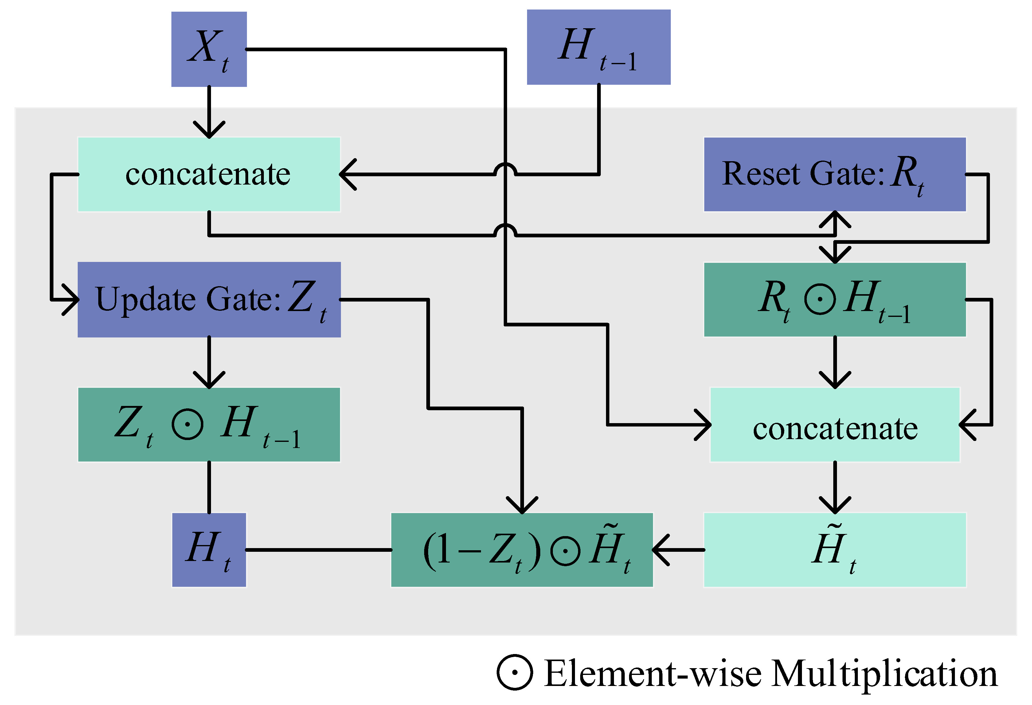
GRU was first proposed by Cho et al. to enhance RNN performance [29] (preprint). As shown in Figure 2, ⊙ denotes the Hadamard product, and σ represents the sigmoid function. At each time step t , GRU receives the current input X t and the previous hidden state H t 1 . It first computes the update gate Z t to determine how much old information to keep and new information to update. Then, it calculates the reset gate R t to decide how much old information to forget. Next, it computes a candidate hidden state based on R t and X t . Finally, it combines old and new information via Z t to produce the current hidden state H ~ t , which is passed to the next step. The GRU’s difference lies in its update and reset gates. These gates work together to dynamically manage information retention and forgetting. This design simplifies the LSTM structure by reducing the number of gates (two in GRU vs. three in LSTM), improving computational efficiency.

2.2.3. Transformer

The Transformer is a deep learning architecture based on attention mechanisms, introduced by Vaswani et al. in 2017 [30]. Departing from traditional RNNs, this model employs multi-head self-attention mechanisms and parallelized computation to efficiently capture long-range dependencies. Its core encoder–decoder structure enables the multi-head attention module to extract features across diverse subspaces, with positional encoding providing temporal awareness. For SST prediction in this study, we optimized the attention heads to 3 through experiments to balance feature interaction depth and computational efficiency. The input dimension is configured as 7, integrating multivariate features: six variables from the dataset plus temporal encodings. The output dimension is set to 1, directly corresponding to the target SST values.

2.2.4. KAN

KAN networks are neural network architectures based on the Kolmogorov–Arnold representation theorem [31]. According to the theorem, any multivariate continuous function can be decomposed into a finite combination of univariate functions.
f ( x ) = q = 1 2 n + 1 ϕ q p = 1 n ϕ q , p ( x p )
where ϕ q , p   is an inner unary function. It processes the p -th component x p   of input vector x independently. It is responsible for nonlinearly transforming original features. ϕ is an outer unary function. It receives the sum of outputs from all inner functions along the same path q and maps it to a scalar value, performing feature fusion and creating higher-order representations. The final output is obtained by combining these outer functions.
Figure 3 contrasts MLP and KAN neural network structures. MLP, based on the universal approximation theorem, positions activation functions at nodes and weights at edges, approximating complex functions via multi-layer structures [32,33]. In contrast, KAN places activation functions at edges and weights at nodes. It computes multivariate functions by combining unary functions, parameterizing them with B-splines. This design addresses MLP’s spectral bias, boosts parameter efficiency and approximation ability, especially for high-dimensional nonlinear problems, and reduces computational complexity [34] (preprint).
B-spline functions, central to the KAN model, replace conventional weight parameters in neural networks [35]. Their flexibility allows adaptation to complex data relationships by shape adjustment, minimizing approximation errors. This enhances the network’s ability to learn subtle patterns in high-dimensional data.
ϕ ( x ) = i = 0 n c i B i , k ( x )
where ϕ ( x ) denotes the spline function, c i represents the spline coefficients optimized by gradient descent, and B i , k x are the B-spline basis functions defined on the mesh.
During training, the spline parameters c i are optimized to minimize the loss function, adjusting the spline’s shape for the best fit to the training data.

2.2.5. GRU_EKAN

GRU_EKAN is an advanced hybrid time series model. Its core innovation lies in the deep integration of GRU with EKAN. The model’s front end uses a standard GRU structure to process input sequences. Through the cooperative action of update and reset gates, it selectively retains historical information and captures temporal evolution patterns. After obtaining the sequence’s final hidden representation, the model abandons traditional linear fully connected layers and instead adopts a multi-layer EKAN structure for non-linear transformation. The EKAN module approximates any complex function using learnable spline basis functions. Its unique dynamic grid adjustment mechanism optimizes spline node positions based on the feature distribution of GRU outputs, effectively solving the “extrapolation” problem of the traditional KAN. It also employs independent channel scaling factors and intelligent initialization strategies based on data distribution. These enhance the model’s ability to perceive feature importance and improve training stability.
The proposed EKAN incorporates two core technological innovations: a dynamic grid adjustment mechanism and channel-wise scaling factors. To precisely align with time series distribution characteristics, the framework implements dynamic grid adjustment by comprehensively sorting GRU output values per feature dimension to identify six equidistant quantiles spanning 0% to 100%, blending these quantile values with a theoretical uniform grid at a 98:2 ratio to form an adaptive topology, and extending three equidistant boundary nodes bilaterally to ensure complete value-domain coverage. Concurrently, channel-wise scaling factors introduce learnable parameters—uniformly initialized in the 0.8–1.2 interval—that dynamically amplify critical features through B-spline output modulation. Fundamentally, this dual-mechanism operates via inverse empirical distribution mapping, transforming uniform nodes through data-driven cumulative distribution functions to create a positive node density–probability density correlation, thereby auto-calibrating resolution in dense regions.

2.3. Model Parameter Settings

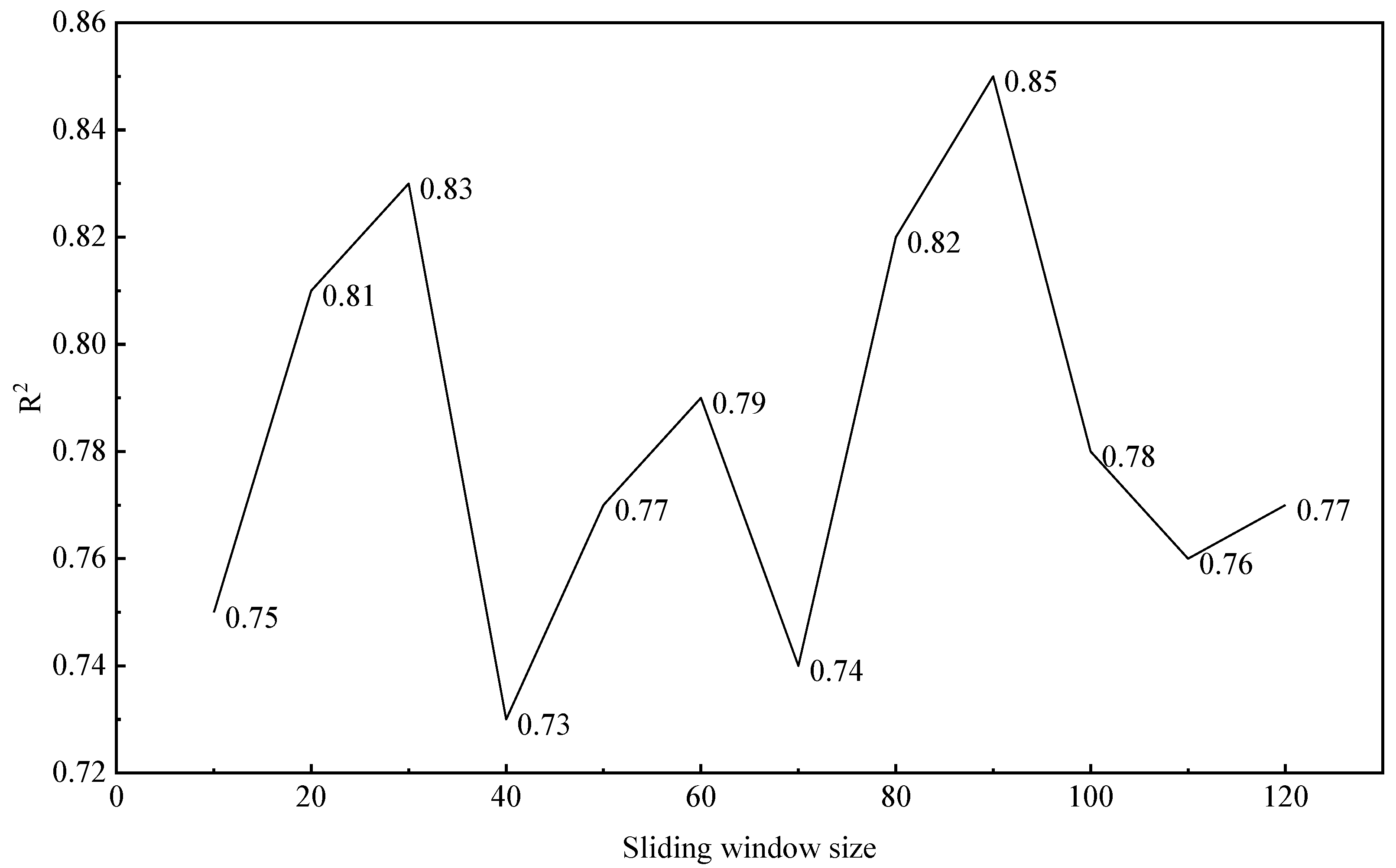
In deep learning, model training involves numerous parameters whose interactions significantly affect prediction accuracy and can lead to substantial variations in outcomes. When determining the sliding window size, we considered the seasonal and cyclical characteristics of the data and initially evaluated window sizes that were multiples of 10. As shown in Figure 4, the results indicated that a 90-day sliding window produced the highest R2 value. Therefore, we adopted this 90-day window size for subsequent modeling. Moreover, since this study employs single-step prediction rather than multi-step prediction, setting the sliding window to 90 days essentially means using the multivariate marine data from the preceding 90 days to predict the SST for the next day.
To ensure the stability and reliability of the experimental results in this study, the same model parameters were used for training and testing in subsequent experiments. Specific parameter settings are detailed in Table 2.
According to the general requirements for deep learning forecasting models [36], the dataset was initially divided into training and testing sets in an 8:2 ratio. To gain a more comprehensive assessment of the model’s predictive performance and optimize the data-splitting approach, the training period (January 2011 to October 2018) was further subjected to a nested splitting strategy. Specifically, this initial training set was split into a training subset (90% of the training set) and a validation subset (10% of the training set). This validation set was crucial for several purposes: computing validation loss to monitor model performance in real time, implementing early stopping when validation loss plateaued, and tuning hyperparameters without compromising the test set (October 2018 to January 2021). This combined approach effectively prevented data leakage and ensured sufficient training data alongside ample testing data for robust model comparison.

2.4. Model Training Process

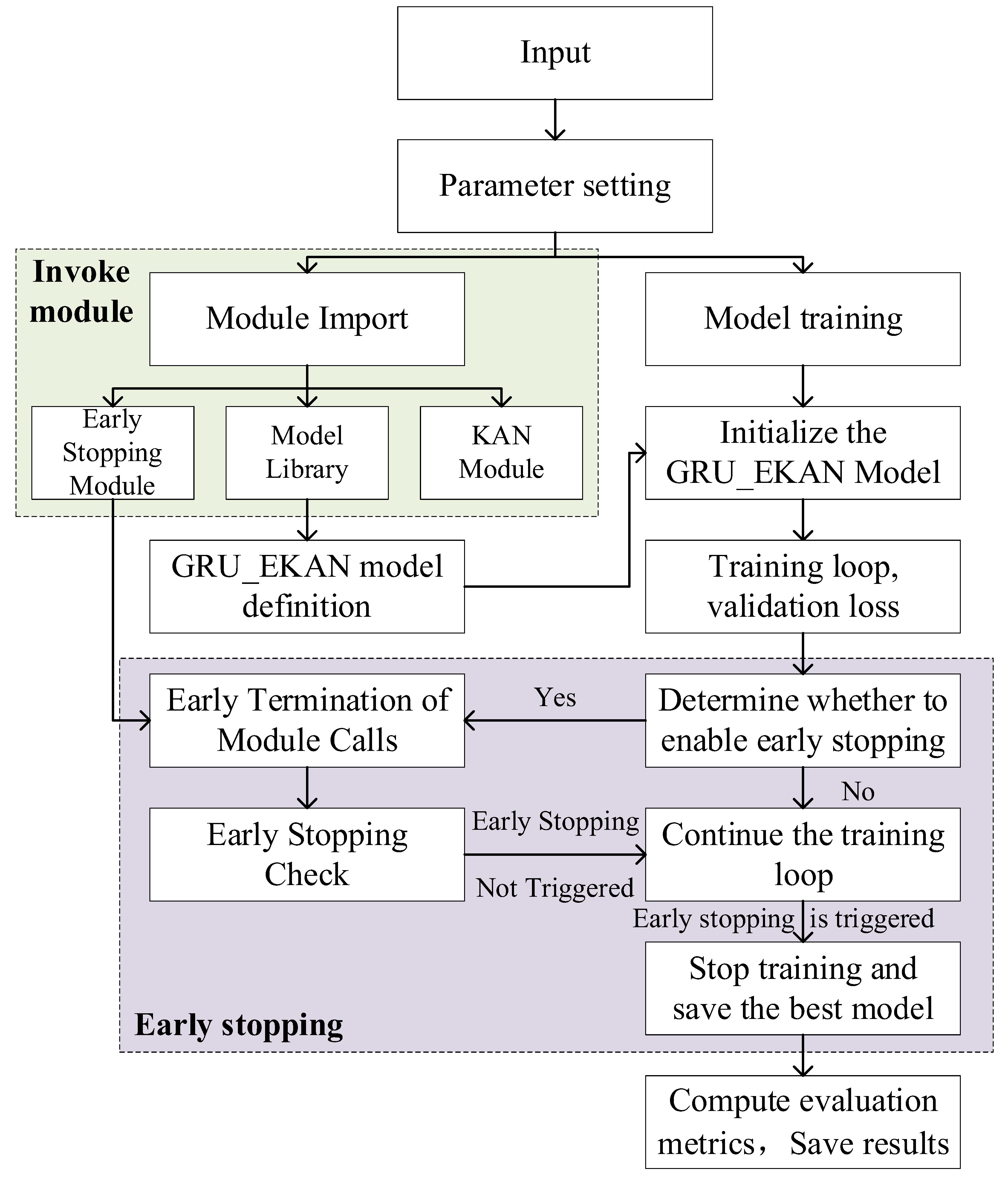
As shown in Figure 5, the model training process of this study is as follows. First, the data were collected and preprocessed. Subsequently, model parameters were configured and the required modules—including early stopping, relevant model libraries, and KAN modules—were imported. The GRU_EKAN model was then defined and initialized, followed by the specification of the loss function and optimizer. During training, model performance was monitored through validation loss calculations, with the early stopping mechanism activated when necessary to mitigate overfitting. Upon training completion, the optimal model was loaded and evaluation metrics were computed. For ablation experiments, models including GRU, LSTM, and LSTM_EKAN were utilized.

3. Results

3.1. Correlation Coefficient Analysis

In marine multivariable regression research, a Pearson correlation coefficient matrix is used to analyze the linear relationships between six variables (bottomT, so, mlotst, uo, vo, and zos) and thetao. The Pearson formula is as follows [37]:
r x y = i = 1 n x i x ¯ y i y ¯ i = 1 n x i x ¯ 2 i = 1 n y i y ¯ 2
where x ¯ and y ¯ denote the means of variables x and y , respectively.
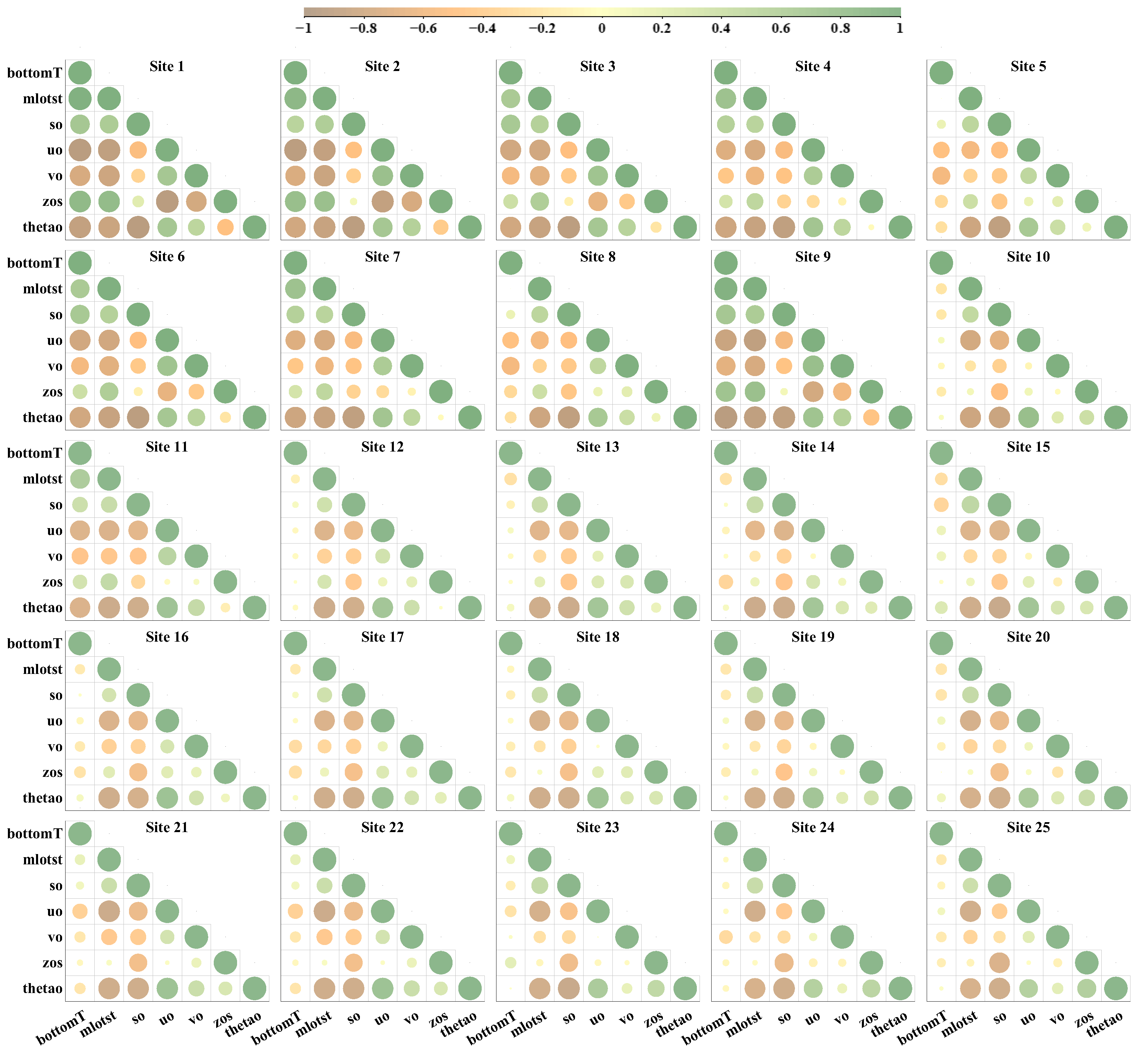
Figure 6 presents a correlation coefficient matrix for 25 sites, utilizing green to denote positive correlations and brown for negative correlations. Within each grid cell, the size of the circular marker indicates the strength of the correlation, with larger circles corresponding to stronger relationships. The results show that theta exhibits a strong negative correlation with bottomT at the initial sites. This suggests that in shallower regions, bottomT is a stable factor influencing the potential temperature structure. Thetao is predominantly negatively correlated with mlotst. The correlation pattern between so and thetao closely mirrors that of mlotst, likely reflecting the influence of intruding cold, saline water masses or upwelling processes. Both uo and vo show positive correlations with thetao, indicating that current velocities are positively associated with sea surface temperature. Overall, the correlation between thetao and zos is weak and shifts from negative to positive across the sites.
Further analysis reveals that the absolute correlation coefficients between all variables and thetao are under 0.6, indicating some linearity exists that may affect model stability and predictive power. To tackle multicollinearity and enhance model stability and generalization, L2 regularization is introduced. It adds a penalty term to the loss function, related to the sum of squares of the model parameters, and the loss function is expressed as [38]:
Loss = 1 n i = 1 n ( y i y ^ i ) 2 + λ j = 1 p β j 2
where 1 n i = 1 n ( y i y ^ i ) 2 is the MSE, λ j = 1 p β j 2 is the L2 regularization term, λ is the regularization parameter, and β j represents the regression coefficients of the model.
In summary, this study used correlation analysis to reveal the relationships between multiple marine variables and thetao. It applied L2 regularization to address multicollinearity, thereby significantly improving the model’s stability and predictive power.

3.2. Comparison of Model Results

This study selects RMSE, MAE, R2, and MSE as evaluation metrics [39,40,41]. MAE measures the model’s overall deviation (stability), MSE identifies large errors in predictions, RMSE indicates the overall error magnitude, and R2 shows the model’s ability to fit overall trends. These metrics reveal the model’s predictive performance from multiple angles, offering a comprehensive understanding of its effectiveness. The specific formulas are as follows:
RMSE = 1 n i = 1 n ( y i y ^ i ) 2
MAE = 1 n i = 1 n | y i y ^ i |
R 2 = 1 i = 1 n ( y i y ^ i ) 2 i = 1 n ( y i y ¯ ) 2
MSE = 1 n i = 1 n ( y i y ^ i ) 2
where y i represents the true sea surface temperature values, y ¯ is their mean, y ^ i denotes the model-predicted temperatures, and n is the total number of data points.
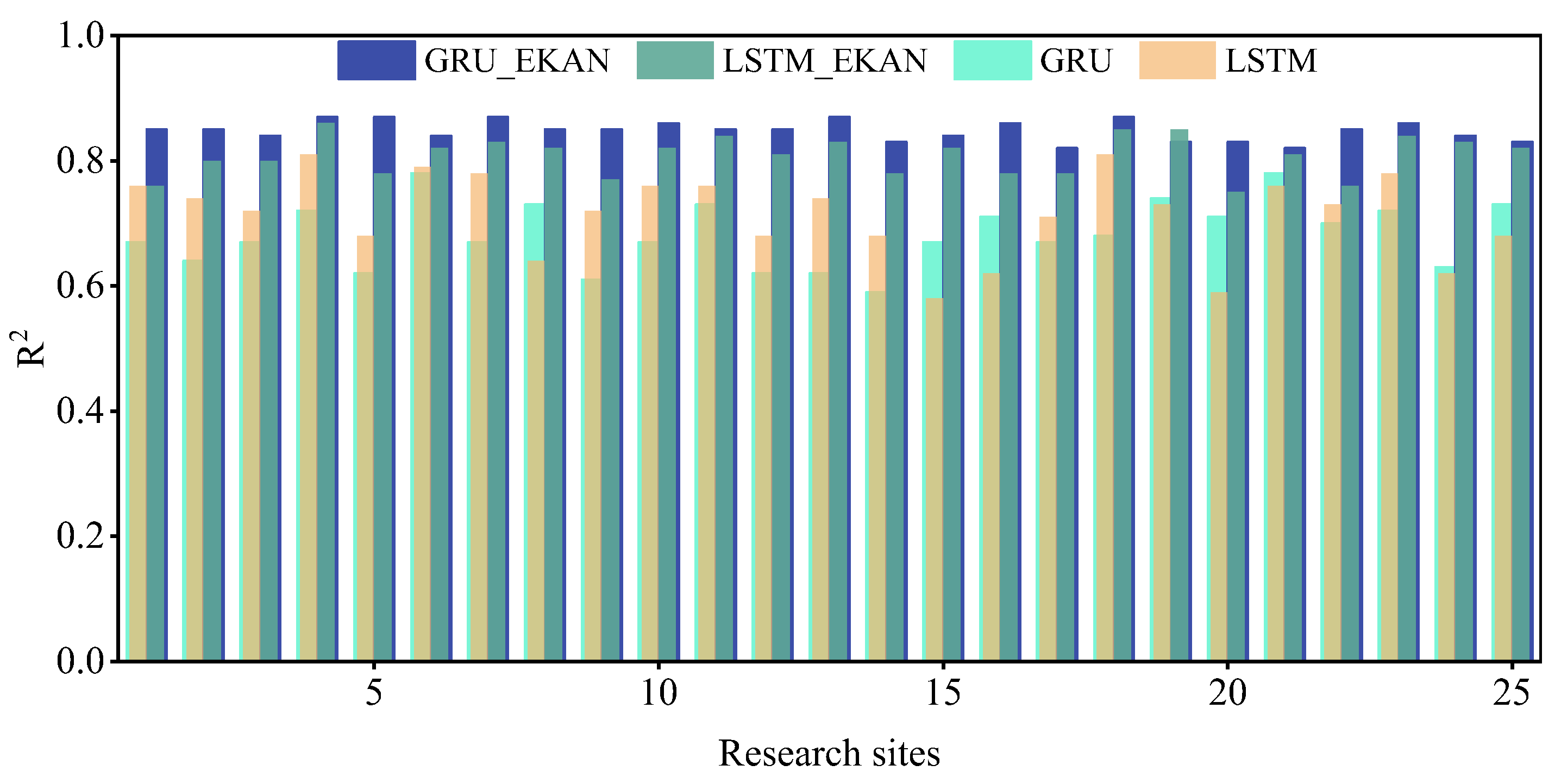
In experiments, even with the same model parameters, multiple tests on the same point can yield different results. To address this, each point was tested three times during training, and the results are shown in Figure 7. The analysis reveals varying predictive performances across the four models (GRU_EKAN, GRU, LSTM, and LSTM_EKAN) at different sites. In terms of average R2 values, GRU_EKAN performs best, followed by LSTM_EKAN, while GRU and LSTM show similar but lower average R2 values. Figure 8 presents boxplots of prediction errors across 25 sites. GRU_EKAN exhibits the narrowest interquartile range, indicating the most concentrated error distribution and superior model stability. With the highest average prediction accuracy (0.85), GRU_EKAN demonstrates significant advantages—surpassing LSTM_EKAN by 6% and GRU by 25%. Meanwhile, LSTM_EKAN shows a 14% improvement over baseline LSTM. Although Transformer achieves a mean value of 0.72, it still trails both GRU_EKAN and LSTM_EKAN, with an 18% deficit relative to GRU_EKAN’s 0.85.
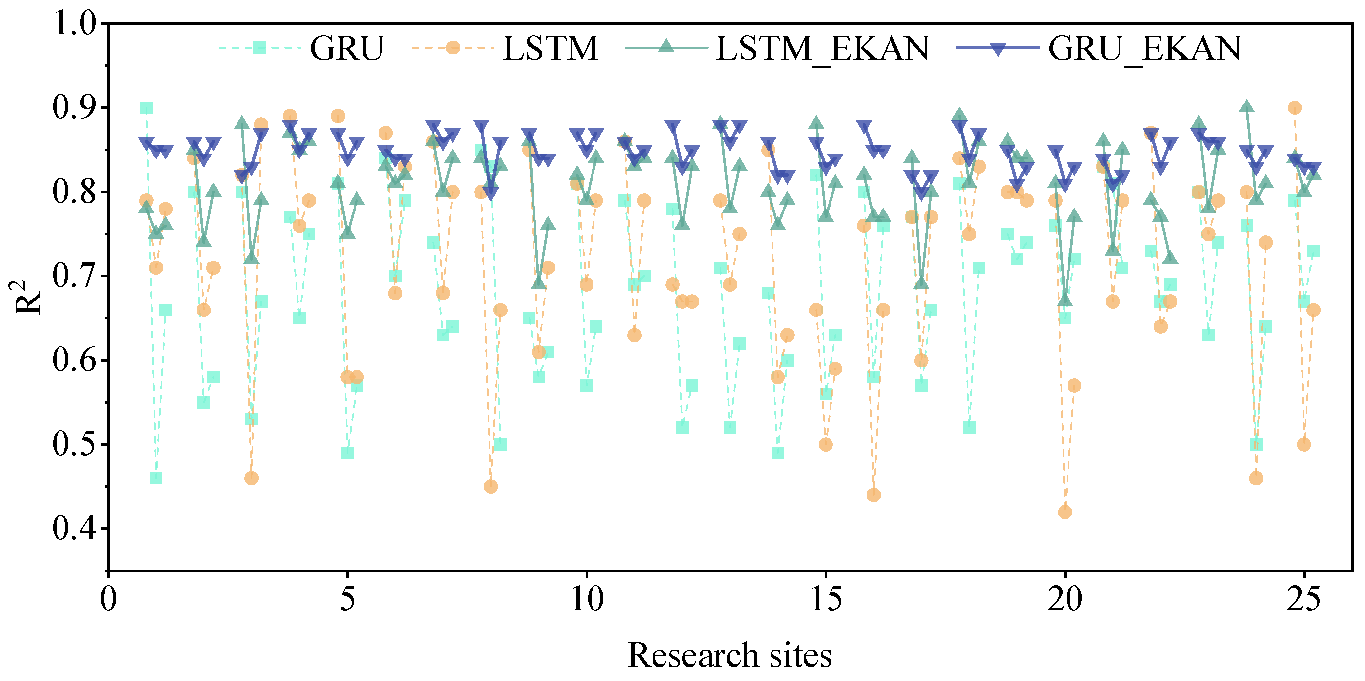
Figure 9 presents the results of a quantitative stability analysis based on repeated experiments conducted at 25 research sites, with each site undergoing three independent trials. The analysis reveals that the GRU_EKAN architecture exhibits superior prediction consistency compared to other models. Specifically, the global R2 standard deviation for GRU_EKAN is 0.019, which is significantly lower than that of GRU (0.121) and LSTM (0.126), representing only 15.7% and 15.1% of their respective values. Notably, the maximum range observed for LSTM was 0.46 at site 15, and the range for GRU was 0.34 at site 2. In contrast, GRU_EKAN maintained a standard deviation of ≤0.025 at these same sites, demonstrating remarkable stability. Furthermore, while the baseline models exhibited high volatility with a range exceeding 0.20 at 60% of the sites, GRU_EKAN consistently maintained a standard deviation of less than 0.03 across all sites. Additionally, the volatility of LSTM_EKAN, measured at 0.049, was 2.58 times higher than that of GRU_EKAN. Importantly, the integration of the EKAN module significantly reduced the median range of GRU by 82.6%, from 0.23 to 0.04, thereby markedly enhancing the consistency of the prediction results.
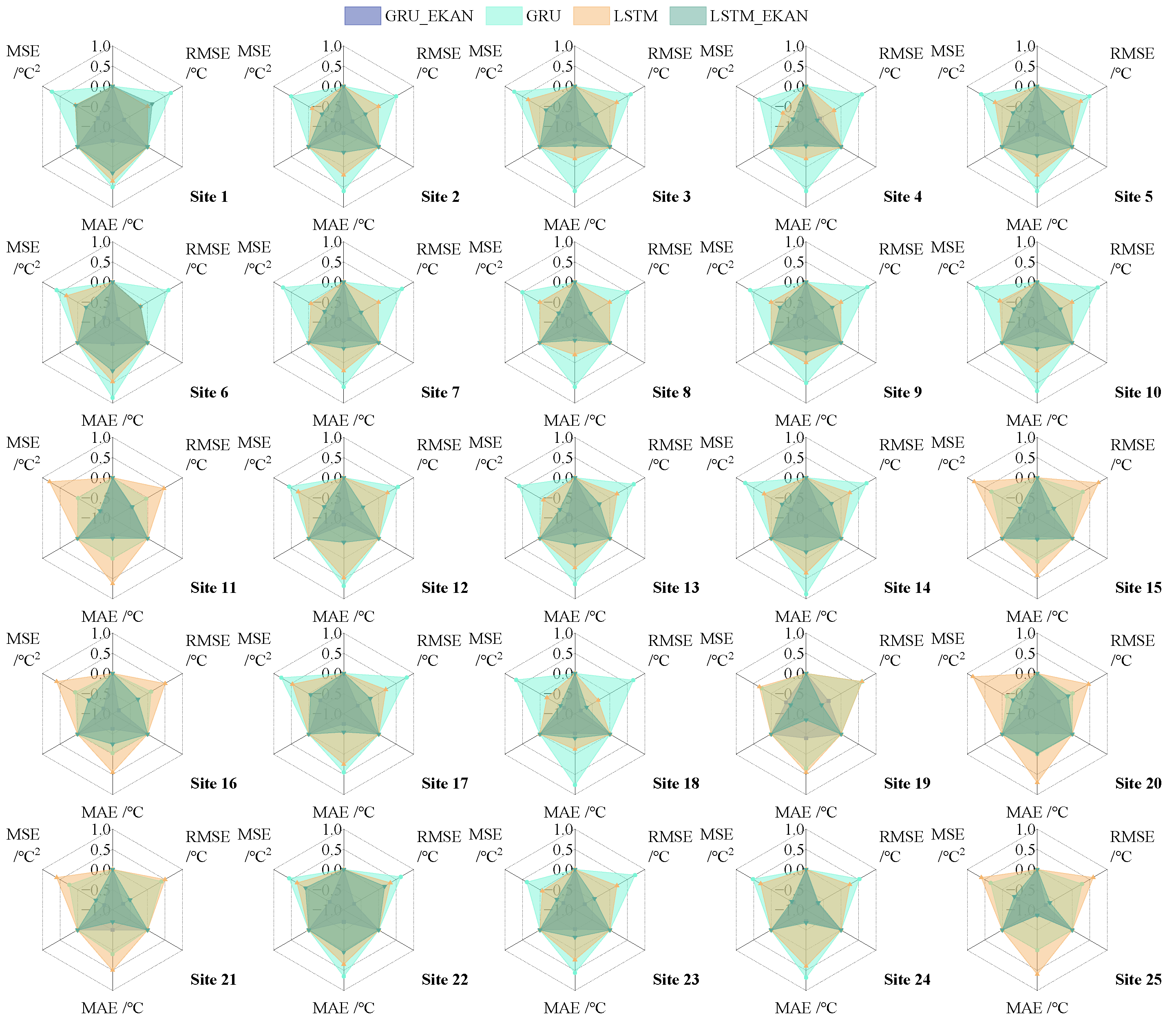
As depicted in Figure 10, the GRU_EKAN model demonstrates superior performance compared to GRU, LSTM, and LSTM_EKAN across the majority of the 25 sites. This is further illustrated by the radar chart, where GRU_EKAN occupies the smallest area, indicating its overall advantage. Although LSTM_EKAN shows a close second, it still trails slightly behind GRU_EKAN. A detailed examination of the accuracy metrics from all 25 sites reveals that GRU_EKAN achieves the lowest average RMSE (0.90 °C), MAE (0.76 °C), and MSE (0.80 °C2). When compared to GRU, GRU_EKAN exhibits substantial reductions of 31.3% in RMSE, 27.0% in MAE, and 53.2% in MSE. Relative to LSTM, the improvements are equally notable, with a 23.1% decrease in RMSE, a 19.9% decrease in MAE, and a 43.3% decrease in MSE. Collectively, these results highlight that GRU_EKAN consistently outperforms the other models, with performance enhancements exceeding 20% across key metrics.
Through a series of evaluation metrics and experimental analyses, this paper comprehensively compares the performance of different models in SST prediction. The results show that the GRU_EKAN model excels in prediction accuracy, stability, and error control, significantly outperforming other models.

4. Discussion

Authors should discuss the results and how they can be interpreted from the perspective of previous studies and of the working hypotheses. The findings and their implications should be discussed in the broadest context possible. Future research directions may also be highlighted.

4.1. WQE Index Analysis

Traditionally, model performance has been assessed through individual metrics such as RMSE and R2. In this study, we introduce the Weighted Quality Evaluation Index (WQE), as proposed by Zhou et al., to provide a more comprehensive evaluation of model performance [24]. The WQE integrates multiple performance metrics, including RMSE, MAE, MSE, and MAPE (Mean Absolute Percentage Error), and assigns specific weights to each metric to derive a composite performance index [39]. This method offers a more accurate representation of the model’s predictive capabilities. The formulas for calculating MAPE and WQE are presented below:
M A P E = 1 n i = 1 n y i y ^ i y i × 100 %
W Q E = 2 X R M S E X m a x X m i n + 3 X M A E X m a x X m i n + M A P E + 4 ( 1 R 2 )
The specific principles for weight assignment are as follows: Given that RMSE is more sensitive to large errors, it is assigned a higher weight (coefficient 2) to emphasize control over significant errors. MAE treats all errors equally and is suitable for scenarios requiring uniform error distribution; therefore, it is assigned the second-highest weight (coefficient 3). MAPE measures relative error but is sensitive to small values; hence, it is assigned a lower weight (coefficient 1) to prevent it from unduly influencing the overall evaluation results. R2 reflects the model’s ability to explain data variation and is a key metric for assessing overall goodness of fit; consequently, it is assigned the highest weight (coefficient 4) to highlight the model’s overall explanatory power. This weighting scheme aims to balance the influence of each metric, enabling the WQE to provide a more comprehensive assessment of model performance and offer a more scientific basis for model selection and optimization.
The findings presented in Table 3 underscore the outstanding performance of the GRU_EKAN model across a range of quality metrics. Notably, within the first five test sites, the GRU_EKAN model consistently delivered WQE values that were significantly lower than those of both the standard GRU and LSTM models, maintaining a stable range between 1.10 and 1.23. This contrasts sharply with the baseline GRU model, which exhibited WQE values ranging from 1.85 to 2.37, and the standard LSTM model, which saw values between 1.18 and 1.90. Furthermore, the GRU_EKAN model outperformed the LSTM_EKAN, another enhanced model, with the latter’s WQE values ranging from 1.03 to 1.58. The only exception was at site 4, where LSTM_EKAN narrowly surpassed GRU_EKAN with a WQE of 1.03 compared to GRU_EKAN’s 1.10. However, even in this instance, GRU_EKAN’s WQE was markedly lower than all other baseline models, with GRU at 1.94 and LSTM at 1.18. A critical aspect highlighted by the data in Table 3 is the remarkable stability of GRU_EKAN’s WQE performance. The model demonstrated a much smaller fluctuation range of 0.13, significantly lower than other models such as GRU (0.52) and LSTM_EKAN (0.55).
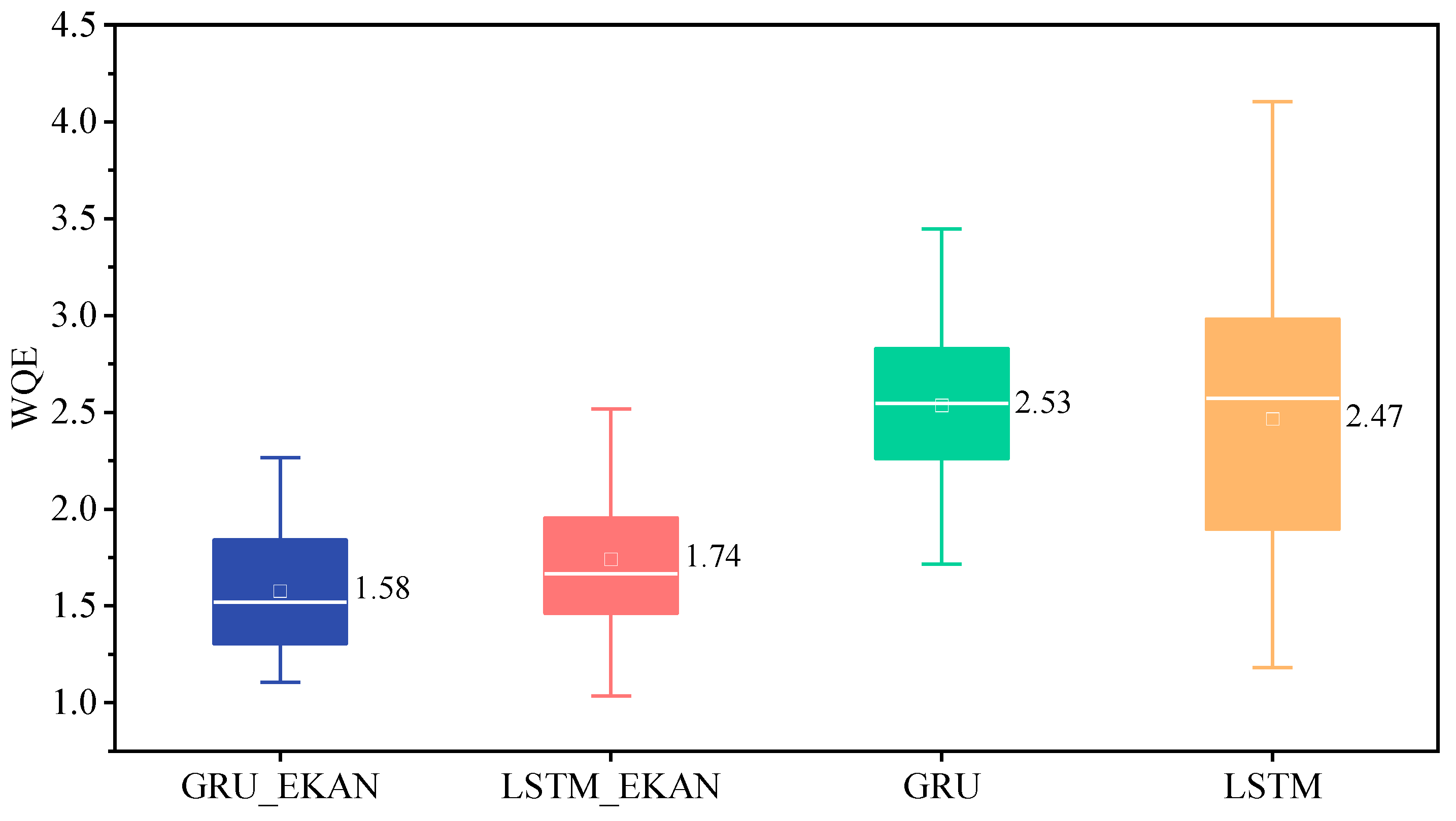
Subsequently, we performed a visual analysis of the WQE outcomes across all sites. Figure 11’s boxplot offers a detailed overview of the WQE performance for the four models—GRU_EKAN, LSTM_EKAN, GRU, and LSTM—across the 25 test sites. The findings reveal that the GRU_EKAN model has the lowest median WQE value at 1.58, highlighting its superior predictive accuracy and stability relative to the other models. Additionally, this model displays a more compact interquartile range and a minimal number of outliers, which further underscores its dependability across diverse conditions. Conversely, the LSTM_EKAN model, with a median WQE of 1.74, although slightly higher than GRU_EKAN, still outperforms the conventional GRU and LSTM models in overall performance. The GRU and LSTM models exhibit median WQE values of 2.53 and 2.47, respectively, which point to a notable shortfall in predictive precision. Furthermore, the broader interquartile ranges and increased frequency of outliers in these models indicate a higher degree of variability in their predictive performance across the various sites.

4.2. Comparison Between Predicted Values and True Values

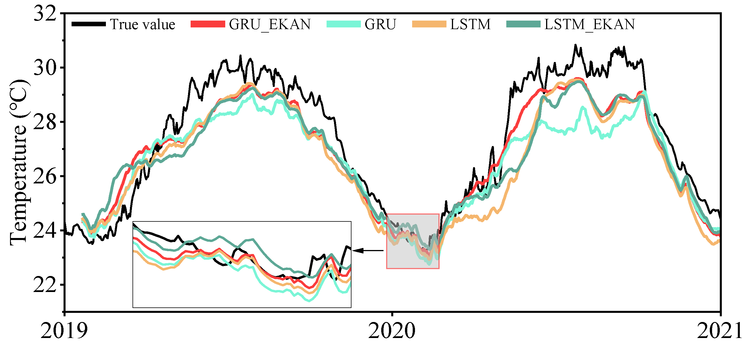
To further evaluate the models’ predictive performance, we compared the predicted values of different models with the actual values, as shown in Figure 11 for site 1. The full dataset covers 25 sites, with results for the remaining 24 in Appendix A. The GRU_EKAN model’s predictions were closest to the observed values at most sites and time periods, especially during high data volatility. Its prediction curve showed smaller fluctuations, closely matching the actual data and demonstrating greater stability. In contrast, while the GRU and LSTM models captured the general trends, they underperformed in prediction accuracy and stability compared to GRU_EKAN.
As shown in Figure 12, the GRU_EKAN model’s predictions are closest to the true values at the beginning and end of the year, indicating high accuracy. However, from early to mid-2019, especially in April and May, the deviation between predictions and true value increases. This is attributed to the combined effects of mid-high latitude circulations and enhanced cross-equatorial flows triggered by the Bay of Bengal cyclone “Fani” in May 2019, causing positive temperature anomalies in the northern SCS [42]. Despite this, the predictions remain relatively close to the true values. Further analysis of 2020 reveals similar mid-year anomalies due to abnormal atmospheric circulation and global warming, leading to a marine heatwave in May [43]. During this period, the model’s predictions show an upward trend first, indicating its ability to capture abnormal temperature changes early for more accurate forecasts.
Through comparative analysis of predicted and actual values across models, the GRU_EKAN model demonstrates superior prediction accuracy and stability, especially during significant data fluctuations. Its early detection of abnormal temperature trends enhances forecast reliability. This highlights the model’s advantages in handling complex marine data and its potential as a robust solution for sea temperature prediction.

5. Conclusions

This study proposed and validated the GRU_EKAN model, a novel hybrid deep learning architecture specifically designed for multivariate SST prediction in the dynamically complex SCS. Simultaneously, the model integrates a GRU network to capture long-term temporal dependencies with an EKAN module to model complex, high-dimensional nonlinear relationships between multiple oceanic variables. L2 regularization was employed within the GRU_EKAN framework to address potential multicollinearity issues identified among predictors through correlation analysis. Quantitative evaluations across 25 spatially distributed SCS monitoring sites demonstrate the significant superiority of GRU_EKAN over all models (GRU, LSTM, and LSTM_EKAN) in multiple key dimensions:
  • Superior Prediction Accuracy and Robustness: GRU_EKAN delivers high-precision predictions with a consistent average R2 of 0.85, demonstrating substantial improvements over benchmark models: 6% higher than LSTM_EKAN (R2 ≈ 0.80), 25% higher than base GRU (R2 ≈ 0.68), 20% higher than LSTM (R2 ≈ 0.71), and 18% higher than Transformer (R2 ≈ 0.72). Furthermore, GRU_EKAN exhibited exceptional stability across diverse locations, evidenced by its markedly lower prediction volatility (global R2 standard deviation = 0.019) compared to GRU (0.121) and LSTM (0.126).
  • Lowest Prediction Errors: GRU_EKAN achieved the best performance across all core error metrics: RMSE = 0.90 °C, MAE = 0.76 °C, MSE = 0.80 °C2. Compared to the base GRU model, this translates to reductions of 31.3% (RMSE), 27.0% (MAE), and 53.2% (MSE). Compared to LSTM, the improvements were 23.1% (RMSE), 19.9% (MAE), and 43.3% (MSE).
  • Highest Comprehensive Predictive Quality: The Weighted Quality Evaluation Index (WQE), synthesizing RMSE, MAE, MSE, and MAPE, unequivocally ranked GRU_EKAN as the best model. It achieved the lowest median WQE value (1.58) across all sites, significantly outperforming LSTM_EKAN (1.74), base GRU (2.53), and LSTM (2.47). Critically, GRU_EKAN also demonstrated the greatest reliability under varying conditions, as shown by its smallest fluctuation in WQE performance (range: 0.13), which was far less than other models (e.g., GRU range: 0.52, LSTM_EKAN range: 0.55).
  • Enhanced Anomaly Detection Capability: During known SCS temperature anomaly events (2019 and 2020), GRU_EKAN predictions were notably closer to observed values than other models. More importantly, it demonstrated a superior ability to detect the onset of abnormal temperature trends earlier, as evidenced during the May 2019 positive anomaly and the May 2020 marine heatwave. Although deviations increased during peak anomaly periods, GRU_EKAN maintained relatively closer tracking than the alternatives.
In summary, the GRU_EKAN model represents a significant advancement in multivariate SST prediction. It demonstrably outperforms traditional GRU, LSTM, Transformer, and the LSTM_EKAN variant in terms of prediction accuracy, stability, error reduction, and overall predictive quality. Its ability to effectively leverage multiple oceanic variables, handle their interdependencies, and accurately capture both normal SST variations and critical climate anomalies like marine heatwaves establishes it as a highly reliable and precise solution for SST forecasting in the complex SCS environment. This high precision is quantitatively evidenced by the model’s superior performance across key metrics: achieving a consistently high mean R2 of 0.85 (significantly exceeding benchmarks by 5–25%), the lowest average prediction errors (RMSE = 0.90 °C, MAE = 0.76 °C, MSE = 0.80 °C2, representing reductions of 23–53% compared to base models), and exceptional stability demonstrated by the smallest R2 standard deviation (0.019) and the best Weighted Quality Evaluation (WQE) Index (median = 1.58). Future work will explore the adaptation and optimization of the GRU_EKAN framework for SST prediction in various marine settings and assess the feasibility of multi-day SST prediction.

Author Contributions

Conceptualization, Z.H.; methodology, Z.H.; code development, X.L.; Hyperparameter tuning, R.S.; validation, S.Z. and H.L.; Writing—original draft, R.S.; Writing—review and editing, Z.H. All authors have read and agreed to the published version of the manuscript.

Funding

This work was sponsored by the National Natural Science Foundation of China (42364002), Natural Science Foundation of Jiangxi Province (20224BAB204065), Innovation Fund for Postgraduates of Jiangxi Province (YC2025-S524), and the Hebei Water Conservancy Research Plan (2022-28).

Data Availability Statement

The ocean reanalysis data used in this study were obtained from the Copernicus Marine Service product Global Ocean Physics Reanalysis (Product ID: GLOBAL_MULTIYEAR_PHY_001_030). This dataset includes temperature, salinity, sea surface height, and associated variables, covering the period January 1993 to June 2021 (accessed on 1 March 2025). The analysis code for this study is openly available in the GitHub repository (V1.0): https://github.com/heimy2000/GTS_Forecaster (accessed on 1 July 2025).

Conflicts of Interest

The authors declare no conflicts of interest.

Appendix A

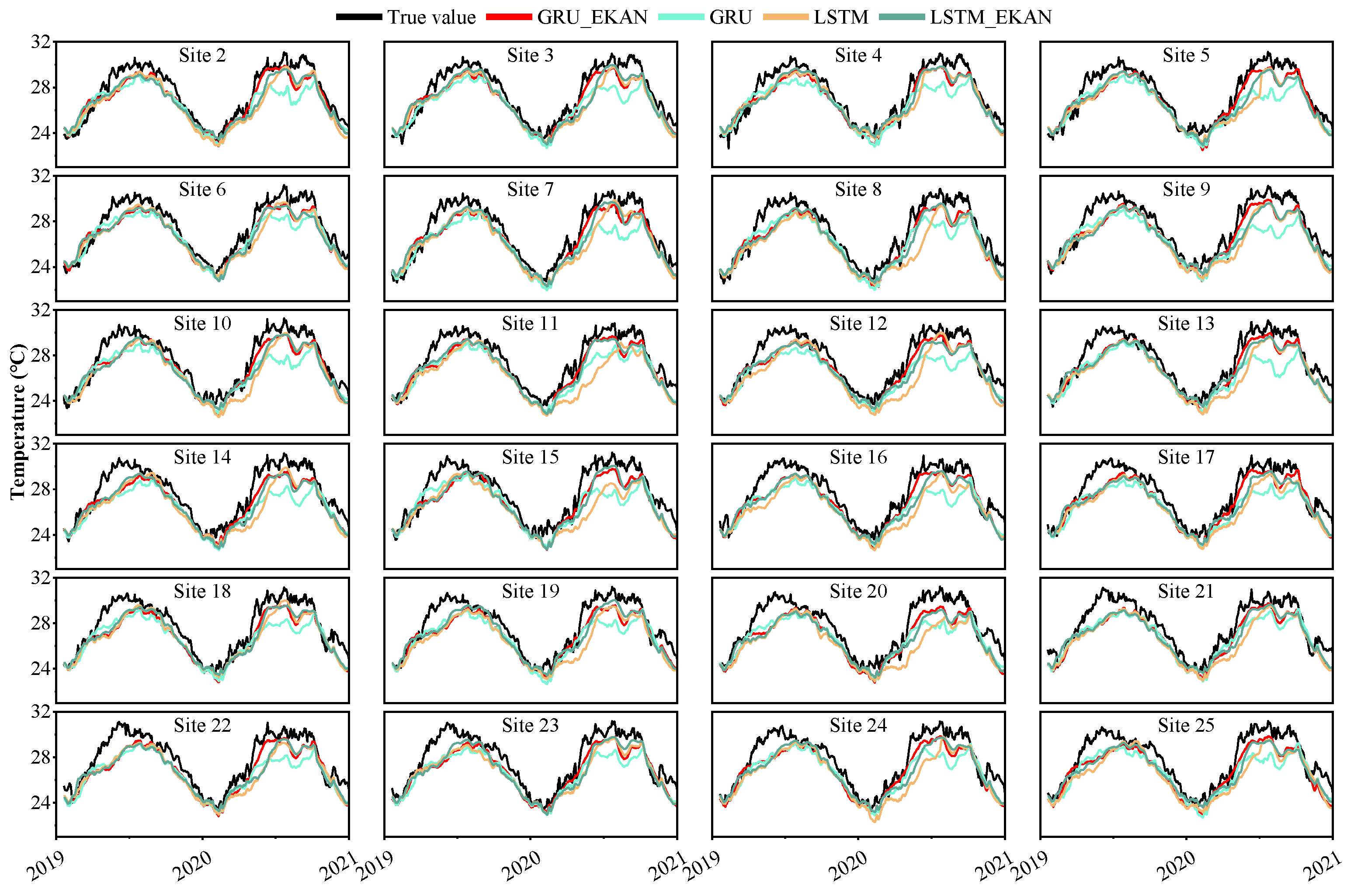
Appendix A presents prediction–result comparison charts for the remaining 24 sites in Figure A1, to offer a more comprehensive understanding of the predictive performance of different models.
Figure A1. Supplement. Comparisons of predicted and actual values for different models at the remaining 24 sites.
Remotesensing 17 02916 g0a1

References

  1. Frankignoul, C. Sea Surface Temperature Anomalies, Planetary Waves, and Air-sea Feedback in the Middle Latitudes. Rev. Geophys. 1985, 23, 357–390. [Google Scholar] [CrossRef]
  2. Deser, C.; Alexander, M.A.; Xie, S.-P.; Phillips, A.S. Sea Surface Temperature Variability: Patterns and Mechanisms. Annu. Rev. Mar. Sci. 2010, 2, 115–143. [Google Scholar] [CrossRef] [PubMed]
  3. Zheng, F.; Zhu, J. Improved Ensemble-Mean Forecasting of ENSO Events by a Zero-Mean Stochastic Error Model of an Intermediate Coupled Model. Clim. Dyn. 2016, 47, 3901–3915. [Google Scholar] [CrossRef]
  4. Dong, B.-W.; Sutton, R.T.; Jewson, S.P.; O’Neill, A.; Slingo, J.M. Predictable Winter Climate in the North Atlantic Sector during the 1997–1999 ENSO Cycle. Geophys. Res. Lett. 2000, 27, 985–988. [Google Scholar] [CrossRef]
  5. Latif, M.; Arpe, K.; Roeckner, E. Oceanic Control of Decadal North Atlantic Sea Level Pressure Variability in Winter. Geophys. Res. Lett. 2000, 27, 727–730. [Google Scholar] [CrossRef]
  6. Rodwell, M.J.; Rowell, D.P.; Folland, C.K. Oceanic Forcing of the Wintertime North Atlantic Oscillation and European Climate. Nature 1999, 398, 320–323. [Google Scholar] [CrossRef]
  7. Venzke, S.; Münnich, M.; Latif, M. On the Predictability of Decadal Changes in the North Pacific. Clim. Dyn. 2000, 16, 379–392. [Google Scholar] [CrossRef]
  8. Chen, Q.; Cai, C.; Chen, Y.; Zhou, X.; Zhang, D.; Peng, Y. TemproNet: A Transformer-Based Deep Learning Model for Seawater Temperature Prediction. Ocean Eng. 2024, 293, 116651. [Google Scholar] [CrossRef]
  9. He, X.; Montillet, J.-P.; Kermarrec, G.; Shum, C.K.; Fernandes, R.; Huang, J.; Wang, S.; Sun, X.; Zhang, Y.; Schuh, H. Space and Earth Observations to Quantify Present-Day Sea-Level Change. Adv. Geophys. 2024, 65, 125–177. [Google Scholar]
  10. Usharani, B. ILF-LSTM: Enhanced Loss Function in LSTM to Predict the Sea Surface Temperature. Soft Comput. 2023, 27, 13129–13141. [Google Scholar] [CrossRef]
  11. Wei, L.; Guan, L. Seven-Day Sea Surface Temperature Prediction Using a 3DConv-LSTM Model. Front. Mar. Sci. 2022, 9, 905848. [Google Scholar]
  12. Xie, J.; Zhang, J.; Yu, J.; Xu, L. An Adaptive Scale Sea Surface Temperature Predicting Method Based on Deep Learning with Attention Mechanism. IEEE Geosci. Remote Sens. Lett. 2019, 17, 740–744. [Google Scholar] [CrossRef]
  13. Ham, Y.-G.; Kim, J.-H.; Luo, J.-J. Deep Learning for Multi-Year ENSO Forecasts. Nature 2019, 573, 568–572. [Google Scholar] [CrossRef] [PubMed]
  14. Wanigasekara, R.; Zhang, Z.; Wang, W.; Luo, Y.; Pan, G. Application of Fast Meemd–Convlstm in Sea Surface Temperature Predictions. Remote Sens. 2024, 16, 2468. [Google Scholar] [CrossRef]
  15. Dai, H.; He, Z.; Wei, G.; Lei, F.; Zhang, X.; Zhang, W.; Shang, S. Long-Term Prediction of Sea Surface Temperature by Temporal Embedding Transformer with Attention Distilling and Partial Stacked Connection. IEEE J. Sel. Top. Appl. Earth Obs. Remote Sens. 2024, 17, 4280–4293. [Google Scholar] [CrossRef]
  16. Dai, H.; Lei, F.; Wei, G.; Zhang, X.; Lin, R.; Zhang, W.; Shang, S. Sea Surface Temperature Prediction by Stacked Generalization Ensemble of Deep Learning. Deep Sea Res. Part Oceanogr. Res. Pap. 2024, 209, 104343. [Google Scholar] [CrossRef]
  17. Yuan, T.; Zhu, J.; Ren, K.; Wang, W.; Wang, X.; Li, X. Neural Network Driven by Space-Time Partial Differential Equation for Predicting Sea Surface Temperature. In Proceedings of the 2022 IEEE International Conference on Data Mining (ICDM), Orlando, FL, USA, 28 November–1 December 2022; pp. 656–665. [Google Scholar]
  18. Yang, J.; Huo, J.; He, J.; Xiao, T.; Chen, D.; Li, Y. A DBULSTM-Adaboost Model for Sea Surface Temperature Prediction. PeerJ Comput. Sci. 2022, 8, e1095. [Google Scholar] [CrossRef]
  19. Du, J.; Nie, J.; Ye, M.; Song, D.; Gao, Z.; Wei, Z. A deep neural networks prediction model for sea surface temperature based on global cross-scale spatial-temporal attention. Chin. J. Mar. Environ. Sci. 2023, 42, 944–954. [Google Scholar]
  20. He, J.; Yin, S.; Chen, X.; Yin, B.; Huang, X. An Informer-Based Prediction Model for Extensive Spatiotemporal Prediction of Sea Surface Temperature and Marine Heatwave in Bohai Sea. J. Mar. Syst. 2025, 247, 104037. [Google Scholar] [CrossRef]
  21. Fan, L.-Y.; Cao, Y.-H.; Huang, N.-Y.; Sun, G.-X.; Cao, J.-N.; Liu, C.-X. OTCFM: A Sea Surface Temperature Prediction Method Integrating Multi-Scale Periodic Features. IEEE Access 2024, 12, 108291–108302. [Google Scholar] [CrossRef]
  22. Chan, J.Y.-L.; Leow, S.M.H.; Bea, K.T.; Cheng, W.K.; Phoong, S.W.; Hong, Z.-W.; Chen, Y.-L. Mitigating the Multicollinearity Problem and Its Machine Learning Approach: A Review. Mathematics 2022, 10, 1283. [Google Scholar] [CrossRef]
  23. Daoud, J.I. Multicollinearity and Regression Analysis. J. Phys. Conf. Ser. 2017, 949, 012009. [Google Scholar] [CrossRef]
  24. Zhou, Y.; He, X.; Montillet, J.-P.; Wang, S.; Hu, S.; Sun, X.; Huang, J.; Ma, X. An Improved ICEEMDAN-MPA-GRU Model for GNSS Height Time Series Prediction with Weighted Quality Evaluation Index. GPS Solut. 2025, 29, 113. [Google Scholar] [CrossRef]
  25. He, X.; Huang, J.; Montillet, J.P.; Wang, S.; Kermarrec, G.; Shum, C.K.; Hu, S.; Wang, F. A Noise Reduction Approach for Improve North American Regional Sea Level Change from Satellite and In Situ Observations. Surv. Geophys. 2025, 47, 1–32. [Google Scholar] [CrossRef]
  26. Fan, Y.; Hu, S.; Sun, X.; He, X.; Zhang, J.; Jin, W.; Liao, Y. Spatial Variation and Uncertainty Analysis of Black Sea Level Change from Virtual Altimetry Stations over 1993–2020. Remote Sens. 2025, 17, 2228. [Google Scholar] [CrossRef]
  27. Hochreiter, S.; Schmidhuber, J. Long Short-Term Memory. Neural Comput. 1997, 9, 1735–1780. [Google Scholar] [CrossRef]
  28. Pascanu, R.; Mikolov, T.; Bengio, Y. On the Difficulty of Training Recurrent Neural Networks. In Proceedings of the International Conference on Machine Learning, PMLR, Atlanta, GA, USA, 16–21 June 2013; pp. 1310–1318. [Google Scholar]
  29. Cho, K.; van Merrienboer, B.; Gulcehre, C.; Bahdanau, D.; Bougares, F.; Schwenk, H.; Bengio, Y. Learning Phrase Representations Using RNN Encoder-Decoder for Statistical Machine Translation. arXiv 2014, arXiv:1406.1078. [Google Scholar] [CrossRef]
  30. Vaswani, A.; Shazeer, N.; Parmar, N.; Uszkoreit, J.; Jones, L.; Gomez, A.N.; Kaiser, Ł.; Polosukhin, I. Attention is all you need. Adv. Neural Inf. Process. Syst. 2017, 30, 5998–6008. [Google Scholar]
  31. Kich, V.A.; Bottega, J.A.; Steinmetz, R.; Grando, R.B.; Yorozu, A.; Ohya, A. Kolmogorov-Arnold Networks for Online Reinforcement Learning. In Proceedings of the 2024 24th International Conference on Control, Automation and Systems (ICCAS), Jeju, Republic of Korea, 29 October–1 November 2024; pp. 958–963. [Google Scholar]
  32. Cybenko, G. Approximation by Superpositions of a Sigmoidal Function. Math. Control Signals Syst. 1989, 2, 303–314. [Google Scholar] [CrossRef]
  33. Hornik, K.; Stinchcombe, M.; White, H. Multilayer Feedforward Networks Are Universal Approximators. Neural Netw. 1989, 2, 359–366. [Google Scholar] [CrossRef]
  34. Liu, Z.; Wang, Y.; Vaidya, S.; Ruehle, F.; Halverson, J.; Soljačić, M.; Hou, T.Y.; Tegmark, M. KAN: Kolmogorov-Arnold Networks. arXiv 2025, arXiv:2501.01234. [Google Scholar] [CrossRef]
  35. Unser, M.; Aldroubi, A.; Eden, M. B-Spline Signal Processing. I. Theory. IEEE Trans. Signal Process. 1993, 41, 821–833. [Google Scholar] [CrossRef]
  36. Shahrabadi, S.; Adão, T.; Peres, E.; Morais, R.; Magalhães, L.G.; Alves, V. Automatic Optimization of Deep Learning Training through Feature-Aware-Based Dataset Splitting. Algorithms 2024, 17, 106. [Google Scholar] [CrossRef]
  37. Asuero, A.G.; Sayago, A.; González, A.G. The Correlation Coefficient: An Overview. Crit. Rev. Anal. Chem. 2006, 36, 41–59. [Google Scholar] [CrossRef]
  38. Hoerl, A.E.; Kennard, R.W. Ridge Regression: Biased Estimation for Nonorthogonal Problems. Technometrics 1970, 12, 55–67. [Google Scholar] [CrossRef]
  39. Hyndman, R.J.; Koehler, A.B. Another Look at Measures of Forecast Accuracy. Int. J. Forecast. 2006, 22, 679–688. [Google Scholar] [CrossRef]
  40. Cameron, A.C.; Windmeijer, F.A. An R-Squared Measure of Goodness of Fit for Some Common Nonlinear Regression Models. J. Econom. 1997, 77, 329–342. [Google Scholar] [CrossRef]
  41. Nagelkerke, N.J. A Note on a General Definition of the Coefficient of Determination. Biometrika 1991, 78, 691–692. [Google Scholar] [CrossRef]
  42. Bao, Y. Mechanisms for the abnormally early onset of the South China Sea summer monsoon in 2019. Acta Meteorol. Sin. 2021, 79, 400–413. [Google Scholar]
  43. Han, T.; Xu, K.; Wang, L.; Liu, B.; Tam, C.-Y.; Liu, K.; Wang, W. Extremely Long-Lived Marine Heatwave in South China Sea during Summer 2020: Combined Effects of the Seasonal and Intraseasonal Variations. Glob. Planet. Change 2023, 230, 104261. [Google Scholar] [CrossRef]
Figure 1. Study area and selected sites.
Remotesensing 17 02916 g001
Figure 2. Structure of the GRU algorithm.
Remotesensing 17 02916 g002
Figure 3. Structural comparison of MLP and KAN.
Remotesensing 17 02916 g003
Figure 4. Test R2 scores for varying sliding window sizes.
Remotesensing 17 02916 g004
Figure 5. Model training process.
Remotesensing 17 02916 g005
Figure 6. Correlation coefficient matrices of 25 sites.
Remotesensing 17 02916 g006
Figure 7. Average R2 of three prediction results for different models.
Remotesensing 17 02916 g007
Figure 8. Boxplots of R2 prediction scores across four models at 25 stations (white dots: mean; white lines: median).
Remotesensing 17 02916 g008
Figure 9. Site-wise R2 values (3 predictions per site, 25 sites).
Remotesensing 17 02916 g009
Figure 10. Comparison of evaluation indicators of GRU_EKAN, LSTM_EKAN, GRU, and LSTM (plotted on a radar chart with three active metrics: RMSE, MSE, MAE, and three blank spokes).
Remotesensing 17 02916 g010
Figure 11. WQE comparison chart of the four models.
Remotesensing 17 02916 g011
Figure 12. Comparison of predicted values and actual values for different models (site 1 as an example).
Remotesensing 17 02916 g012
Table 1. Overview of selected parameters from the GLOBAL_MULTIYEAR_PHY_001_030 dataset.
ParameterDescription
bottomTSea water potential temperature at sea floor (°C)Resolution: 1/12° horizontal resolution
Data assimilation: reduced-order Kalman filter
The correction of large-scale biases in temperature and salinity: 3D-VAR
mlotstOcean mixed layer thickness defined by sigma theta (m)
soSea water salinity (g/kg)
uoEastward sea water velocity (m/s)
voNorthward sea water velocity (m/s)
zosSea surface height above geoid (m)
thetaoSea water potential temperature (°C)
Table 2. Hyperparameter settings of the model.
HyperparameterModel Setting ValueDescription
Training set2851Training data for model training (January 2011–October 2018)
Test set713Test data for evaluating the performance of the model (October 2018–January 2021)
Learning rate0.001Hyperparameter controls the step size of model parameter update.
Hidden size64The dimension of the hidden layer
Input size7The dimension of the input layer
Output size1The dimension of the output layer
Seq len90The length of each sliding data window
Batch size32The batch input at one time in the time series data
Table 3. Statistical comparison of prediction errors for different models (with the first five sites serving as examples).
SiteModelMAERMSEMAPER2WQE
1GRU_EKAN0.750.872.69%0.861.11
LSTM_EKAN0.911.113.25%0.781.58
GRU0.991.233.48%0.721.85
LSTM0.961.143.46%0.761.67
2GRU_EKAN0.730.912.62%0.851.15
LSTM_EKAN0.861.023.08%0.811.39
GRU1.061.363.70%0.662.17
LSTM0.961.133.45%0.761.64
3GRU_EKAN0.790.942.83%0.831.23
LSTM_EKAN0.851.023.05%0.801.39
GRU1.111.383.91%0.642.26
LSTM0.971.143.47%0.751.68
4GRU_EKAN0.750.892.68%0.851.10
LSTM_EKAN0.690.852.48%0.861.03
GRU1.031.273.60%0.691.94
LSTM0.750.932.48%0.831.18
5GRU_EKAN0.720.902.59%0.841.16
LSTM_EKAN0.861.033.06%0.791.46
GRU1.101.363.87%0.622.37
LSTM0.961.133.39%0.711.90
Disclaimer/Publisher’s Note: The statements, opinions and data contained in all publications are solely those of the individual author(s) and contributor(s) and not of MDPI and/or the editor(s). MDPI and/or the editor(s) disclaim responsibility for any injury to people or property resulting from any ideas, methods, instructions or products referred to in the content.