Article

Assessing Kernel-Driven Models’ Efficacy in Urban Thermal Radiation Directionality Modeling Using DART-Simulated Scenarios

1
ICube Laboratory, UMR 7357, CNRS-University of Strasbourg, 300 bd Sebastien Brant, CS 10413, F-67412 Illkirch Cedex, France
2
State Key Laboratory of Efficient Utilization of Arable Land in China, Institute of Agricultural Resources and Regional Planning, Chinese Academy of Agricultural Sciences, Beijing 100081, China
*
Author to whom correspondence should be addressed.
Remote Sens. 2025, 17(16), 2884; https://doi.org/10.3390/rs17162884
Submission received: 14 July 2025 / Revised: 14 August 2025 / Accepted: 17 August 2025 / Published: 19 August 2025
(This article belongs to the Section Urban Remote Sensing)

Abstract

The intensification of the urban thermal environment has brought attention to urban land surface temperature (ULST). Complex building geometry and manmade material lead to significant thermal radiation directionality (TRD) of the urban canopy, and the TRD effect directly influences the accuracy of ULST retrieval algorithms. Therefore, it is essential to understand and eliminate the TRD effect to achieve high-accuracy ULST. In this context, the hemispherical brightness temperature maximum–minimum discrepancy (BTD) was quantitatively analyzed via different spectral bands, component temperature thresholds, urban geometries, and component temperature differences. Meanwhile, the DART simulations database was used to systematically evaluate 1 single-kernel- and 30 dual-kernel-driven models (KDMs), which were combined from 5 base-shape kernels (RossThick, Vinnikov, uea, RossThin, and LSF) and 6 hotspot kernels (RL, Roujean, Vinnikov, LiSparseR, LiDense, and Chen). Results show that the BTD discrepancy (ΔBTD) can reach up to 0.91 K with different band emissivities, whereas the ΔBTD is over 10 K with different component temperature differences. The building density and ratio between building heights and road widths (H/W) also exhibit their importance over urban regions. In addition, the RossThick–/Vinnikov–Roujean dual-kernel KDMs demonstrate better performance with an overall RMSE of 1.12 K. The RL-series KDMs can describe the hotspot distribution well, but the uea-series KDMs outperform at the solar principal plane (SPP) and cross-solar principal plane (CSPP). Specifically, the performance of all KDMs is sensitive to the H/W and component temperature thresholds, and urban geometry can affect the TRD RMSE with increasing H/W and a depletion of high building density. The quantitative TRD analysis and comparison provide a comprehensive reference for understanding the distribution of thermal radiation, which is also a reliable basis for developing the new TRD model over urban regions.

1. Introduction

Thermal radiation directionality (TRD) significantly affects the land surface temperature (LST) applications in monitoring extreme weather events, urban heat island effects, and urban thermal environments [1,2,3,4,5,6]. The TRD causes the incomparability of LST in different observation directions, which significantly constrains the application of LST. The influence of such a phenomenon on urban LST is more profound due to complicated ground geometry structures and various manmade materials [5,7,8,9,10]. The available measurement also demonstrated that urban TRD can reach 10 K, which exceeds the accuracy required of LST retrieval [11,12,13,14]. Therefore, it is important to quantify the TRD and investigate the key influencing factors on TRD in urban areas.
Many pioneers have developed some TRD models to eliminate the TRD influence on LST applications, including physical models and semi-empirical kernel-driven models (KDMs). Several physical models were derived from the thermal radiative transfer (TIR) theory. The TITAN model developed a radiative model considering the solar radiation and thermal emission, which aimed to quantify the radiative contributions of all components within a customizable pixel. It emphasized that the reflection and emission of walls are inevitably taken into account in the calculation of TRD over urban regions [11]. Based on a similar urban scenario, ATIMOU-series models were developed by considering adjacent radiation from the influence of urban geometry structures. They systematically proposed and coupled the thermal transfer equation of each component and displayed directional brightness temperature (DBT) within view zenith angles (VZAs) of 50° [15,16]. However, these physical models are derived based on specific scenarios with complicated expressions. In contrast, the minimal input requirements and acceptable accuracy make KDMs the primary selection in TRD-related studies [11]. Most KDMs were originally developed for different land covers within the natural ground, a few of which were designed for urban surfaces. The KDMs for natural surfaces can be grouped into two categories. The first category is a refinement of the visible and near-infrared (VNIR) bidirectional reflectance distribution function (BRDF) framework, where the DBT is usually used instead of the reflectance [17,18,19,20,21]. The reflectance is sensitive to varying solar illumination, whereas LST cannot immediately respond to the appearance/disappearance of the solar illumination. Given the characteristic difference between reflectance and LST, the GOg model was developed by considering the component temperature differences and the conversion between land surface components with thermal inertia [22]. The second category is directly constructed by thermal infrared radiation (TIR) theory, and the addition of emissivity kernels provides sufficient rationale for the acquisition of DBT in the TIR field [23,24,25,26,27].
Urban ground geometry is different from natural ground, and some studies have explored the KDM applied to urban surfaces. Sun et al. revised the emissivity kernel in [24] by an assumption of the urban isothermal surface; after that, they adopted the CoMSTIR simulation data to evaluate the proposed usea kernel [28]. Likewise, based on the hypothesis that urban buildings are the protrusions with equal heights, random locations, and orientations, the GUTA-series KDMs have been deduced with the neglect of mutual shadowing onto the ground [29,30,31]. In particular, the GUTA-Sparse model focused on the influence of vertical walls on the TRD and adopted three classifications via the relative location between the solar and observation for quantifying the contribution of walls [32]. In addition, the GUTA-Dense model was developed to compensate for the flaws of the GUTA-Sparse model at higher building density [33]. Thereafter, Bian et al. proposed an analytical model by considering the single scattering between urban main components, and they adopted geometric optical theory to calculate the direct radiation of sunlit/shadowed roofs/walls/roads [34].
Though some TRD studies have already been developed, there are still some problems to be explored. On one hand, the comparisons of KDMs are always carried out on natural surfaces, and it is not clear whether those well-behaved KDMs could be used to characterize urban TRD [35,36,37]. On the other hand, it is not comprehensive because these satellite data may cause errors with limited view angles and inconsistent sensor platforms [27,38,39,40]. Additionally, some models were not specifically developed for urban regions in the TIR spectra. Therefore, it is important to evaluate the performance of KDMs for understanding the urban TRD characteristics, which also provides new insights into the improvement of TRD models over urban regions.
Based on the Discrete Anisotropic Radiative Transfer (DART) model, this study aims to clarify the key influencing factors on TRD in urban areas, and to recognize the strengths and weaknesses of the classical available KDMs. Section 2 presents a detailed description of simulation metadata, scenarios, and parameter settings. Section 3 presents the modeling assumption and theory of classical KDMs, including base-shape kernels and hotspot kernels. Then, the TRD is analyzed with multiple influencing factors, and the simulation database is used to evaluate 31 KDMs in Section 4. Finally, this study points out its limitations and summarizes the conclusions.

2. Study Area Materials

2.1. DART Model

The Discrete Anisotropic Radiative Transfer (DART) model was developed by the Center for Space Exploration of the Earth’s Biosphere (CESBIO) in 1992 [41]. It is one of the most sophisticated and comprehensive 3D simulation models, including Flux-tracking, Monte Carlo, and LiDAR. It can simulate the radiative transfer between the atmosphere and land surface from the ultraviolet to thermal infrared bands. It can also be coupled with 3DMAX, ILWIS, and SCOPE models to refine natural and urban scenarios for more realistic simulation results. In addition, the DART-EB mode was exploited to calculate the urban 3D radiative budgets, and it was evaluated by the CAPITOUL project measurements with considerable precision in Toulouse districts [42]. The DART model is frequently improved and optimized to obtain a better performance, whose band radiance error is less than 0.2 K in the Earth Observation thermal infrared bands [43]. Recently, DART-Lux with the new Monte Carlo method can provide accurate and fast simulation of satellite images [44]. Meanwhile, it can output the sunlit/shadow ratios and surface temperature of each triangle or square when solar illumination is present in the radiation simulation. It is convenient for users to conduct experiments and analyze complex terrain areas without real data. Due to its excellent performance in complex underlayment, DART simulation results are frequently used in complicated radiation studies as a reference [5,31,32,33,45,46]. Therefore, DART was selected to simulate the urban TRD effect and evaluate the available kernel-driven models. The simulation configuration (as shown in Table 1) includes surface temperature properties, spectral variables, and urban topography structures, and each facet is Lambertian within the urban landscapes. In this study, it should be noted that atmospheric radiation is not considered in the TRD simulation, in order to quantify the influence of land surface parameters.

2.2. Airborne LST Data of the DESIREX 2008 Campaign

The DESIREX 2008 campaign carried out a series of ground- and airborne-based measurements to support the development of urban thermography studies, and it was organized by the European Space Agency (ESA) during the period from 25 June to 4 July 2008 in Madrid, Spain. The AHS spectrometer was carried on the aircraft with five ports of different spectral bands, and there were 10 LWIR bands in port 4 with an average FWHM of 450 nm. A configuration of 7 LWIR bands was used to obtain the LST by applying the Temperature Emissivity Separation (TES) algorithm, and the supervised classification image for each flight line was also obtained from this campaign [47,48,49]. In this study, the statistical LSTs of a two-pass flight pattern at noon were selected as the reference for the DART simulation. It is noted that some natural surface types (water and vegetation) are not considered due to the limited analysis, and the special thermal conductivity of metal makes it not representative in this study. Though it is easy to distinguish land cover from these airborne data with higher spatial resolution, they are not always comprehensive and ideal. Each land cover of LST was extracted to remove outliers with confidence intervals of 5–95%. Nevertheless, it is still challenging to determine the accurate pixel temperature and magnitude of each component (sunlit/shadowed roofs/walls/roads). Therefore, these LSTs are generalized and set as the combination of average surface temperature (AST) and varying temperature thresholds (ΔT) based on the statistical data. Since the temperature difference between components is important for TRD research [50], this study uses different ΔT values (5 K, 10 K, and 15 K) to diagnose the performance of available KDMs. DART can operate and assign reasonable pixel temperatures based on urban geometry structures, ΔT, and AST. The incorporation of the airborne LST data ensures that all component temperatures are set within reasonable ranges, thereby enhancing the reliability of simulation results. This configuration aims to conveniently and quantitatively analyze the urban TRD in as realistic urban scenarios as possible.

2.3. Spectral Properties

The ECOSTRESS spectral dataset has been updated from the ASTER spectral library with many spectral functions for classic natural and urban land covers, and it is frequently used to obtain land surface emissivity in LST-retrieving algorithms [51,52,53]. In this study, four classical manmade materials (asphalt, concrete, brick, and glass) were selected as the building materials for simulation urban landscapes, and their spectral functions are shown in Figure 1a. Meanwhile, these four spectral functions are convolved with the spectral response function of ECOSTRESS to obtain the simulation surface emissivity of each material, and the emissivity of 5 bands is shown in Figure 1b. Notably, the initial emissivity is set only based on subpixel surface material, and it is independent of the urban geometry structures and component temperatures.

2.4. Simulation Scenarios

In addition to building surface temperatures and material emissivity, the digital surface model (DSM) is important for obtaining an urban TRD simulation database. There is always a lack of urban DSM datasets with high spatial resolution, and a realistic DSM is too intricate to quantify the magnitude of influencing factors for urban TRD. Fortunately, Morrison et al. pointed out that it is valid when the simplified surface temperature and cuboid buildings are used to model LST TRD, and the bidirectional behavior of the scenario is not insensitive to the exact building shapes [53,54]. They demonstrated that LST TRD modeling is not constrained to idealized descriptions of urban morphology. Therefore, this study used simplified buildings and fixed roads to simulate urban landscapes.
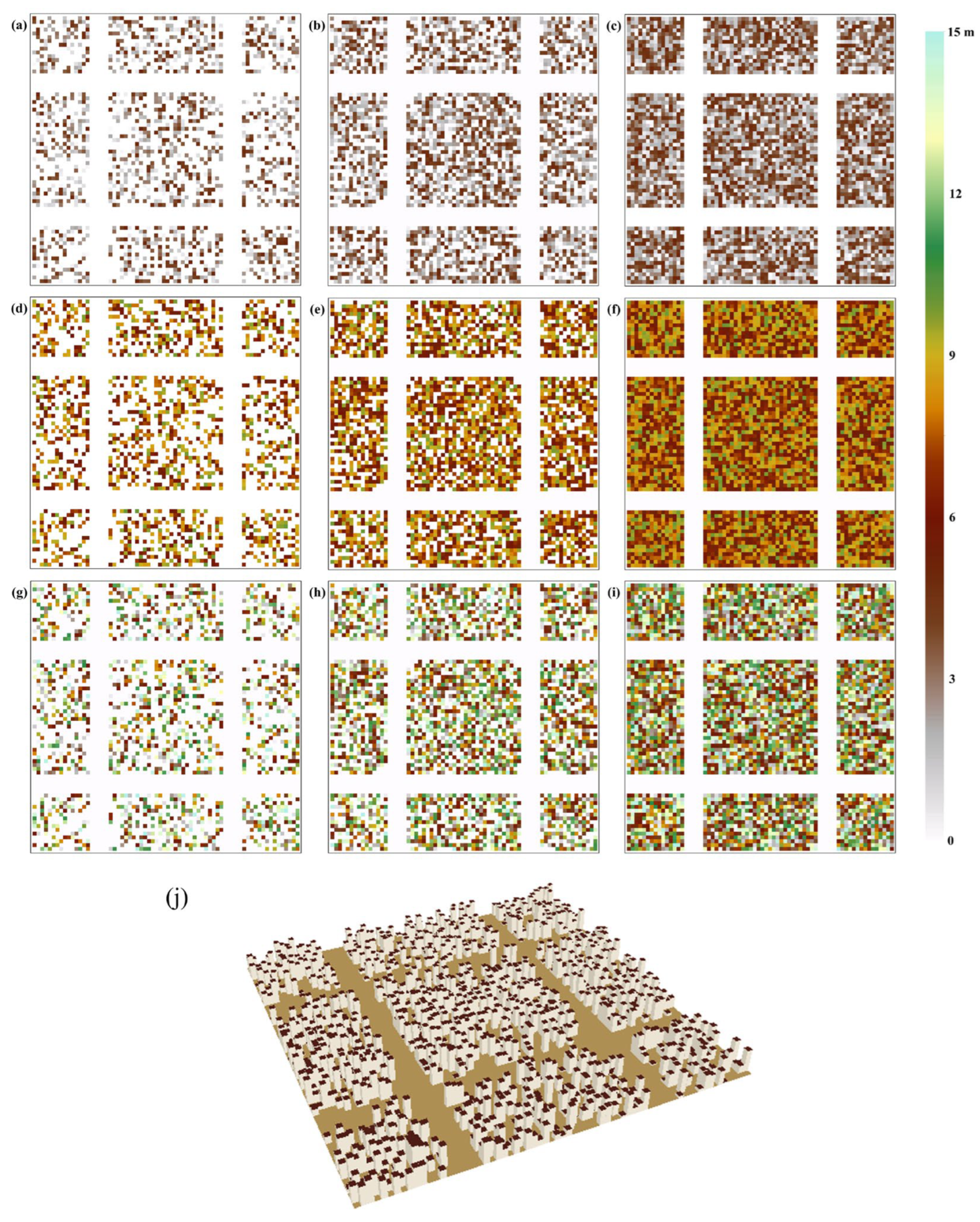
In this study, the simulation scenes were set as a 70 m × 70 m square to match an ECOSTRESS pixel scale, and the whole urban landscapes were generated via random building distribution and heights accompanied by four fixed roads. In detail, two north–south roads and two east–west roads of 5 m width were distributed at a fixed location, and there were four intersection points. The distribution of buildings was randomly assigned in the remaining areas according to building density, and the randomized building heights were regulated by the adoption of given ranges. As shown in Figure 2, the building density in each row increases from left to right, whereas the average building height in each column increases from top to bottom. Finally, there are nine urban landscapes with a combination of three building densities (0.29, 0.50, and 0.73) and three building height ranges (0~5 m, 5~10 m, and 0~15 m), and different ratios between building heights and road widths are also included here (0~1, 1~2, and 0~3). For convenience, they are referred to as S1, S2, S3, S4, S5, S6, S7, S8, and S9 in the latter sections. Furthermore, the 3D visualization of S1 is presented in Figure 2j, providing a more intuitive depiction of the simulated urban scenes. Other simulation scenes are not presented here due to their structural similarity with S1.

3. Kernel-Driven Models

To compare the differences between available TRD models, all the kernel-driven models are written in a uniform form [23]:
T θ s , θ v , φ = f i s o + f B a s e S h a p e K B a s e S h a p e + f H o t s p o t K H o t s p o t
where T is the directional brightness temperature (DBT), θs is the solar zenith angle (SZA), θv is the view zenith angle (VZA), φ is the relative difference (RAA) between the solar azimuth angle and the view azimuth angle, fiso is an isotropic kernel that represents the Lambertian surface, fBaseShape is the base-shape kernel that describes the volume-scattering radiation within the landscapes, fHotspot is the hotspot kernel that represents the radiation distribution of the landscapes based on the geometry structures, and KBaseShape and KHotspot are coefficients of the base-shape kernel and the hotspot kernel, respectively. Other models that cannot be parameterized in this form (Equation (1)) are not considered in this study.
These classical TRD models can be decomposed into two categories based on Equation (1), and available base-shape kernels and hotspot kernels are described below.

3.1. Base-Shape Kernel

(1)
RossThick kernel [29,55]
The formula of the RossThick kernel was taken from [56], whose derivation is based on the bidirectional reflectance model above the horizontal plant canopy with single-scattering radiation. This formula was initially applied to scenarios with a large leaf area index (LAI). Therefore, it adopted the approximation of an optically thick canopy, which causes the dominating role of LAI and the minor role of view angles during the procedure of the simplified equation. Finally, this kernel is defined as
K R T k = π / 2 ξ cos ξ + sin ξ cos θ s + cos θ v π 4
cos ξ = cos θ s cos θ v + sin θ s sin θ v cos φ
where KRTk is the RossThick base-shape kernel, and ξ is the phase angle calculated by the geometry among solar, surface, and observation locations.
(2)
Vinnikov kernel [24]
The expression of this emissivity kernel is derived from nighttime observations of two geostationary satellites. It assumes that the LST of an arbitrary satellite is consistently biased compared to that of other observations, and the expression can be written in a form that excludes solar radiation. The emissivity kernel is fitted using two zenith angles of satellite observations, and it may comprise many functions with various shapes. Their universal shape can be found by the least squares method, which is written as
K V i n B = 1 cos θ v
where KVinB is the emissivity kernel of the Vinnikov model.
(3)
usea kernel [28]
Based on the Vinnikov emissivity kernel, Sun et al. proposed that the realistic ULST distribution within a mixed pixel is close to an isothermal surface, and the anisotropy of the usea model is mainly due to the multi-scattering at nighttime. Therefore, the usea emissivity kernel can be simplified to a form with the view zenith angles:
K u e a = sin θ v
where Kuea is the emissivity kernel of the usea model.
(4)
RossThin kernel [55]
The RossThin kernel was designed to apply at small LAI, whose derivation method is similar to that of the RossThick kernel. However, it adopted the approximation of an optically thin canopy, and the photon scattering term beneath the canopy was replaced by the average Lambertian reflectance. Its kernel can be written as
K R T i = π / 2 ξ cos ξ + sin ξ cos θ s cos θ v π 2
where KRTi is the RossThin kernel.
(5)
LSF kernel [25]
The LSF kernel proposed the concept of apparent emissivity increment, which is caused by ground geometry structures and non-isothermal subpixels. Meanwhile, this concept explains the directional and spectral dependence in LST. Based on the BRDF, the emissivity term is derived from Taylor’s first-order expansion of the Planck function, and this conceptual kernel can be written as
K L S F = 1 + 2 cos θ v 0.96 + 2 0.96 cos θ v 1 4 cos θ v 1 + 2 cos θ v + 0.15 1 exp 0.75 / cos θ v
where KLSF is the LSF kernel.

3.2. Hotspot Kernel

(1)
RL kernel [18,57]
This hotspot kernel follows the Poisson model, which is derived from the photon distribution probability between foliage. It divides the scenarios into several sublayers and calculates their extinction coefficients via the coupling of the ingoing and outgoing transmittances. The temperature difference between off-nadir and nadir directions replaced the reflectance in [57], and the optical kernel has been successfully utilized in the thermal infrared field:
K R L = exp k f exp k tan θ s 1 exp k tan θ s
where KRL is the hotspot kernel, k is related to the different hotspot widths (its value equals 2 here), f is the geometric distance based on the cosine theorem, and it can be calculated by
f = tan 2 θ s + tan 2 θ v 2 tan θ s tan θ v cos φ
(2)
Roujean kernel [29]
This kernel assumes that the subpixel is composed of protrusions with the same shape and size, and the mutually shadowed regions between protrusions are neglected. In this model, the wall orientations are taken into account, which are associated with the wall surface irradiance. This geometric scattering kernel was originally designed for the bidirectional reflectance simulation, and it has been recently used to evaluate the urban thermal anisotropy given its similarity to buildings [38]. Its formula is written as
K R o u = 1 2 π π φ cos φ + sin φ tan θ s tan θ v 1 π tan θ s + tan θ v + f
where KRou is the Roujean hotspot kernel.
(3)
Vinnikov kernel [24]
Based on the procedure of the Vinnikov emissivity kernel, its solar kernel can be fitted by the daytime data from two geostationary satellites, and θs and φ are used to quantify the solar radiation and hotspot effect. The Vinnikov solar kernel can be written as
K V i n H = sin θ v sin θ s cos θ s cos φ cos θ s θ v
where KvinH is the hotspot kernel of the Vinnikov model.
(4)
LiSparseR kernel [55,58]
This kernel is developed from the model of [59], and it assumes that the directionality only depends on the illuminated components (equally bright), and the shadowed crown and ground are perfectly dark. Meanwhile, this kernel employs the assumption of the elliptical crown to replace the spherical crown, and its final form is written as
K L S R = O θ s , θ v , t sec θ s sec θ v + 0.5 1 + cos ξ sec θ s sec θ v
where KLSR is the LiSparseR kernel, O(θs,θv,t) is the overlap parts of sunlit and viewed elliptical areas, t is the intersection points of these two ellipses, θ * and ξ′ are the angles of deformation in the elliptical geometry, and they practically refer to the same concepts as the θ* and ξ of other kernels. The calculation of these parameters is similar to the spherical crown, and a detailed description is shown in [55].
(5)
LiDenseR kernel [55,58]
The crown structure of random heights in [25] is selected to derive the LiDenseR kernel, and they introduce the ratio value between sunlit viewed crown and shadow background areas. In the dense vegetation canopy, this added parameter leads to the variation in the LiSparseR kernel model. With the same derivation method, the LiDenseR kernel can be written as
K L D R = 1 + cos ξ sec θ s sec θ v sec θ s + sec θ v O θ s , θ s , t 2
where KLDR is the LiDenseR kernel.
(6)
Chen kernel [60]
Based on the canopy gap distribution, this kernel was developed to improve the semi-empirical model of [29], and this hotspot kernel was used to compensate for the hotspot effect around the solar illumination. The magnitude and width of the hotspot are defined as two coefficients with land covers and canopy features. The smaller variations in these parameters make this model widely applicable to all land covers, and it means that this simple KDM can fulfill the application of global requirements. The magnitude of these coefficients is regarded as a constant due to the limited building landscapes, and B = 0.01 in this study.
K C h e n = exp ξ / ( B π )
where KChen is the Chen hotspot kernel.
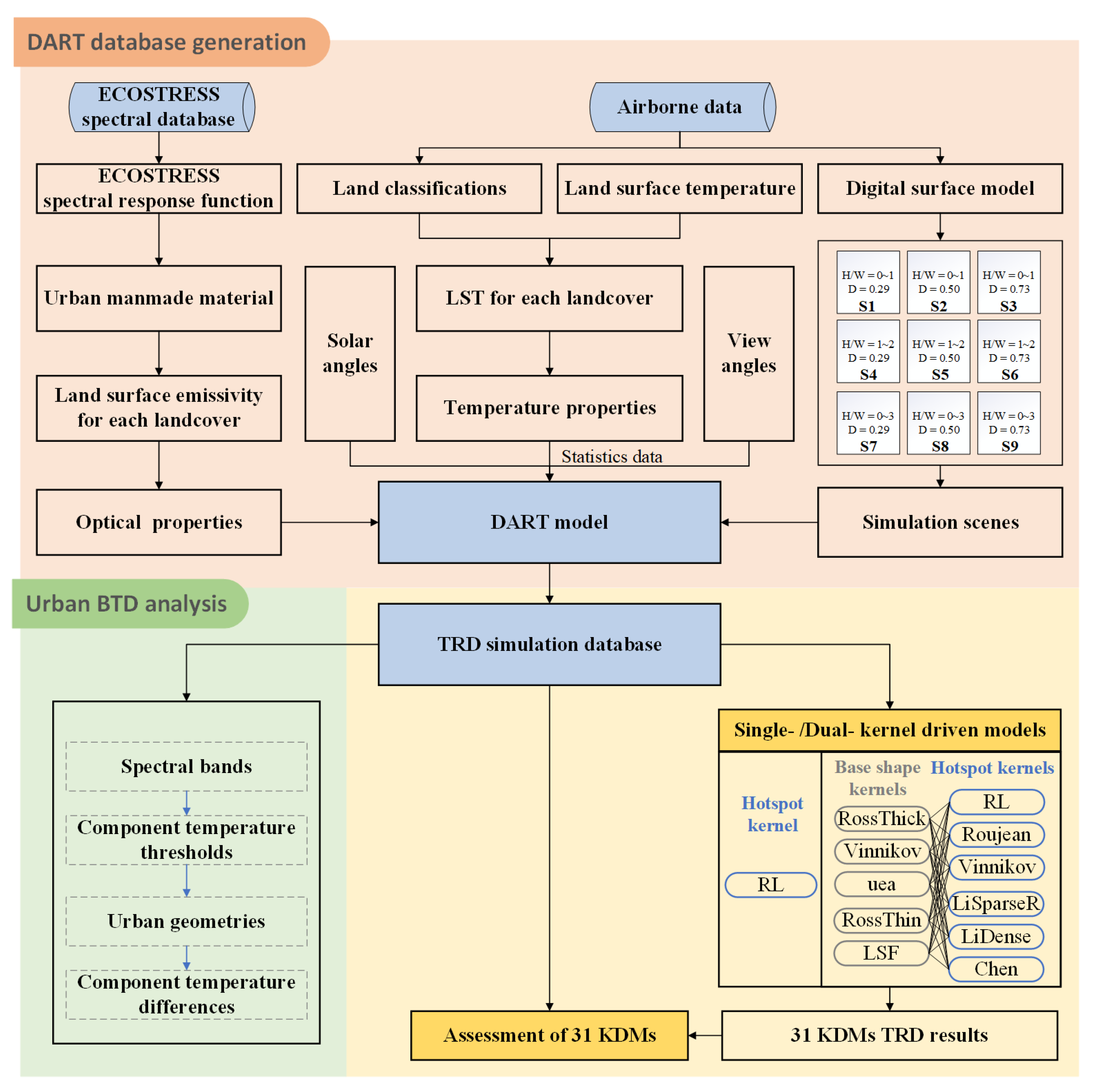
These base-shape kernels and hotspot kernels are arranged and combined to obtain 31 KDMs, including 1 single-kernel model (RL) and 30 dual-kernel models. In this process, some new models are derived from these classical kernel-driven models, and all KDMs are numbered and listed in Table 2. Firstly, the airborne data is statistically used to generate the DART simulation database. The urban brightness temperature maximum–minimum discrepancies (BTD = BTmax − BTmin) are employed to analyze the directional extremum of thermal variation across the hemispherical domain. Finally, the DART TRD simulations are used to evaluate the performance of 31 KDMs. The main flowchart is shown in Figure 3.

4. Results and Analysis

4.1. Analysis of DART Simulation Dataset

4.1.1. The BTD in Different ECOSTRESS Spectral Bands

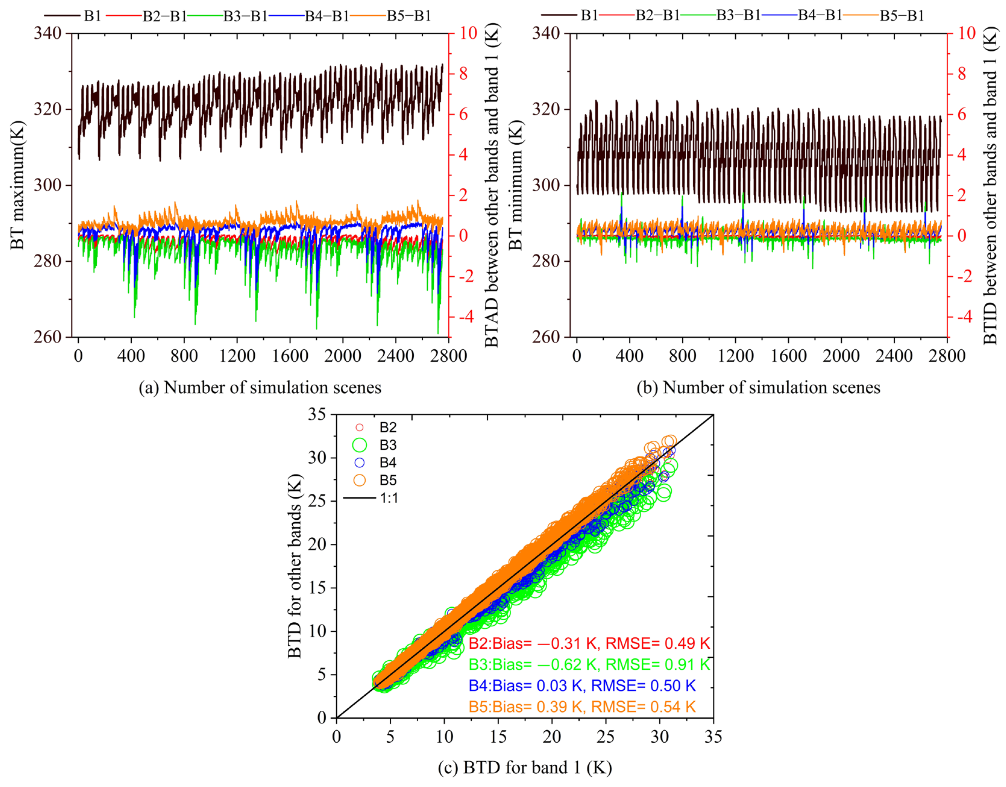
According to the radiative transfer equation in the TIR field, the surface emissivity plays an important role in ULST retrieval. To analyze the influence of different band emissivities, this study selected five ECOSTRESS TIR bands as typical TIR bands, and the brightness temperature maximum–minimum discrepancy (BTD) was employed to quantify the directional extremum of thermal variation across the hemispherical domain. The BTD of band 1 was regarded as a reference for the evaluation of inter-band differences. It is important to recognize the BTD of band 1 before the comparison between different TIR bands, and the brightness temperature (BT) maximum and minimum of band 1 are shown in Figure 4a,b with black lines. The BT maximum has a stepped-increasing trend, and the BT minimum shows an opposite stepped-decreasing trend. This phenomenon is related to the configuration of component temperature thresholds (ΔT), which in the DART were set as 5 K, 10 K, and 15 K, respectively. It is undeniable that the higher temperature threshold results in a wider temperature range, which causes the higher BT maximum and lower BT minimum. Meanwhile, Figure 4a,b demonstrate the BT maximum discrepancy (BTAD) and BT minimum discrepancy (BTID) between other bands and band 1. As shown in Figure 4a, the BT maximum of band 2 is closer to that of band 1, and the BTADs in all simulations are within −1 K. The largest BTAD occurs between band 3 and band 1, and its value even reaches up to −4 K under some situations. The BTAD of band 4 ranges from −3 K to 1 K, and that of band 5 is always greater than 0 K. There are similarities in the trend of BTAD between band 2 and band 3, as well as band 4 and band 5, and it is due to the varying differences in band emissivities in conjunction with Figure 1b. In addition, the BTIDs in different bands are always stable around 0 K, and they do not show an obvious trend in Figure 4b.
Based on the BT maximum and BT minimum across the hemispherical domain, it is easy to obtain the BTDs of different bands. Figure 4c shows the BTD scatterplots to explore the influence of different band emissivities. Compared with the BTD of band 1, the overall bias and RMSE are −0.31 K and 0.49 K in band 2, −0.62 K and 0.91 K in band 3, 0.03 K and 0.50 K in band 4, and 0.39 K and 0.54 K in band 5. The peak of BTD discrepancy (ΔBTD) occurs at band 3, and it is due to the higher band emissivity differences between band 1 and band 3. The magnitude of BTAD is significantly larger than that of BTID, which demonstrates that the band emissivity affects the BT maximum more than the BT minimum across the hemispherical domain. It exhibits the importance of band emissivity for the BTD, which has been frequently ignored in the previous urban TRD study.
In addition, the BT maximum and minimum of band 1 can also be divided into distinct groups corresponding to different simulation scenes, as shown in Figure 4a,b with black lines. This grouping pattern indicates that there are other parameters affecting the BT, which subsequently affect the BTD. Therefore, the BTD of band 1 is employed to further investigate these influencing factors in all simulation scenes, and it will be discussed in the following sections in detail.

4.1.2. The BTD in Different Component Temperature Thresholds

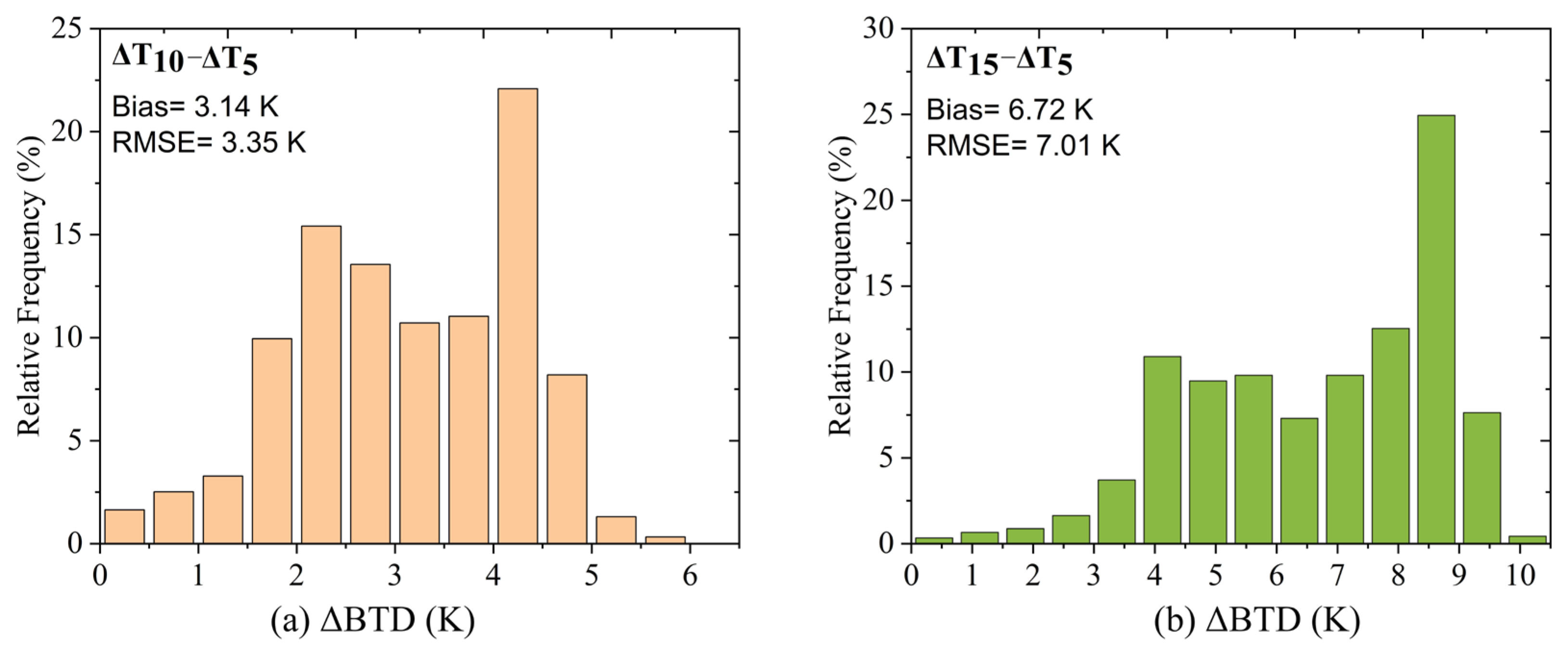
The influence of band emissivity on the BTD is primarily mediated through its effect on the BT maximum, and the BT maximum is related to the component temperature thresholds (ΔT). In this section, the BTD discrepancy (ΔBTD) between 5 K component temperature thresholds (ΔT5) and 10 K/15 K component temperature thresholds (ΔT10/ΔT15) is analyzed via the statistical histogram. Figure 5 shows the ΔBTD between different ΔT groups and ΔT5 in ECOSTRESS band 1. In conjunction with Figure 4, as ΔT increases, the BT maximum increases and vice versa. Although there seems to be a linear trend in changes in BT maximum and minimum, the influence of ΔT is not constant. Based on the frequency of distribution in the histogram, the ΔBTDs of ΔT15 and ΔT10 show irregular variations, which means that ΔT may affect the ΔBTD along with other parameters of simulation scenes. The bias and RMSE of ΔBTD between ΔT10 and ΔT5 are 3.14 K and 3.35 K, and the bias and RMSE of ΔBTD between ΔT15 and ΔT5 are 6.72 K and 7.01 K. In addition, the ΔBTD between ΔT15 and ΔT5 is higher than that between ΔT10 and ΔT5, and their RMSEs differ by a factor of two. The comparison between different groups indicates that the ΔT has a greater influence than band emissivities on the urban TRD study.

4.1.3. The BTD in Different Urban Geometries

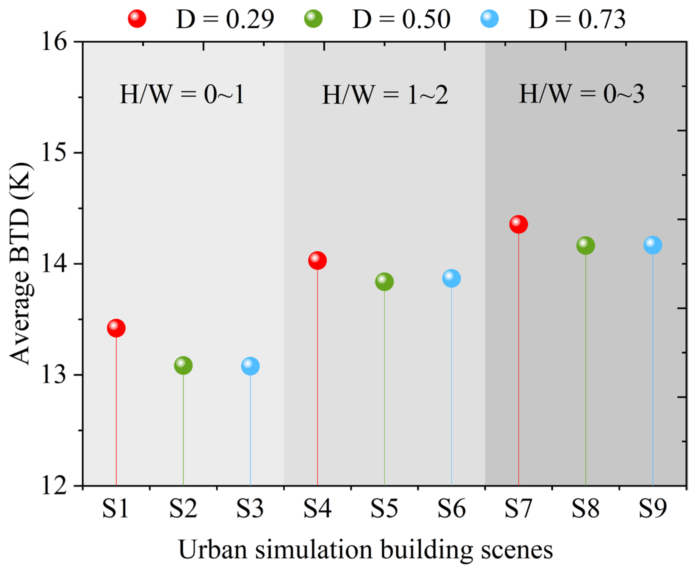
In this study, the urban building scenes were statistically simplified into nine simulation urban building scenarios, and various building densities (D) and ratios between building heights and road widths (H/W) were employed to characterize the heterogeneity of the urban surface. It is noted that the H/W of S1, S2, and S3 range from 0 to 1, the H/W of S4, S5, and S6 range from 1 to 2, and the H/W of S7, S8, and S9 range from 0 to 3. Additionally, S1, S4, and S7 have a building density of 0.29, S2, S5, and S8 have a building density of 0.5, and S3, S6, and S9 have a building density of 0.73. In this section, the arithmetic mean is employed to facilitate the analysis of the band 1 BTD across different urban landscapes. Results show that the BTD in different urban simulation scenarios varies significantly, and the BTDs of nine urban landscapes are 13.41 K, 13.08 K, 13.07 K, 14.02 K, 13.83 K, 13.86 K, 14.35 K, 14.16 K, and 14.16 K, respectively. As shown in Figure 6, the BTD increases when the H/W ranges from 0~1 to 0~3, and the BTD decreases with the increasing building density. The overall ΔBTD between different H/W is higher than that between different building densities. The magnitude of ΔBTD can reach up to 1.09 K with the same building densities and different H/W, and the building density can only cause a maximum of 0.33 K variation when its range is from 0.29 to 0.50. Specifically, the BTD remains stable when the building density reaches up to a critical value with the same H/W. It indicates that the influence of urban H/W is more profound than building densities in denser urban types, and both the building densities and H/W should be considered in the TRD study over the sparse urban scenes.

4.1.4. The BTD in Various Component Temperature Differences

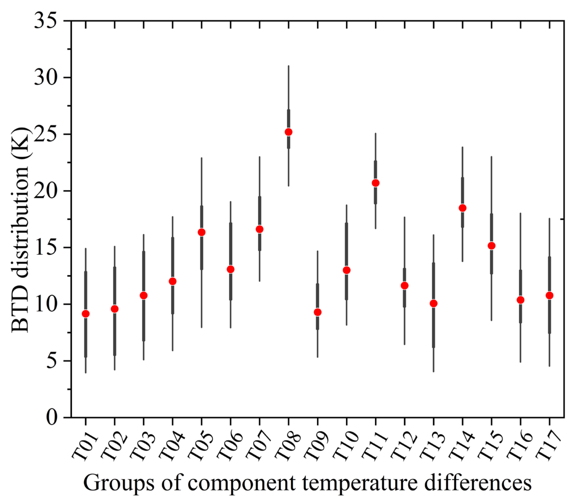
Compared with band emissivities and urban geometries, the ΔT significantly influences BTD, and it is directly related to the component temperature differences. Therefore, component temperature differences are cited as the vital influence factor on the BTD, and the roof, wall, and road are selected as the main urban components without the support of other ancillary data in this study. To analyze the influence on the BTD conveniently, all simulations are divided into 17 groups whose classifications are shown in Table 3. Meanwhile, BTD distributions of different groups are demonstrated in Figure 7. As shown in Figure 7, the larger component temperature difference causes a concentrated BTD distribution, while it is dispersed with the smaller component temperature difference. In the hemispherical space, the BTD is sensitive to component temperature differences, and such a phenomenon is conspicuous between different groups. There is a BTD maximum in T08 whose component temperature difference between roads/roofs and walls is larger than in other groups. When two components within the walls, roads, and roofs maintain the same average surface temperature (AST), the average BTD increases by the gradual increment of δT1/δT2, and the BTD peak exists at the δT1/δT2 of 20 K (T01~T05). The minimum road surface temperature exists in T05, T08, T11, and T14, and the larger temperature differences cause their higher BTDs. The maximum road surface temperature exists in T02, T09, T12, and T15, whose BTD is gradually increased by diminishing wall surface temperature, and it shows that the increasing component temperature differences may be more important than component temperatures themselves. The minimum wall surface temperature exists in T15, T16, T17, and T01, whose BTD is 15.24 K in T15, and the BTD of the other groups is about 10 K without significant variations. The maximum wall surface temperature exists in T02, T06, T07, and T08. The BTD exhibits notable variations by increasing δT2/δT1 and invariant δT1/δT2, and the ΔBTD can reach up to 15.85 K between the groups of T02 and T08. In addition, the hotspot shapes and locations of simulations will vary with different component temperature differences, which also explains their importance. The above results indicate that component temperature differences have a significant impact on the BTD values and distributions. It also implies that most KDMs might be inaccurate when directly used in thermal infrared fields from the optical spectrum. The analysis of ΔT and component temperature differences demonstrates the influence of component temperature on the BTD from different perspectives, which indirectly highlights the importance of component temperature in the TRD study.

4.2. Comparison Between Kernel-Driven Models and DART Simulation TRDs

4.2.1. The Performance of Kernel-Driven Models in All Simulations

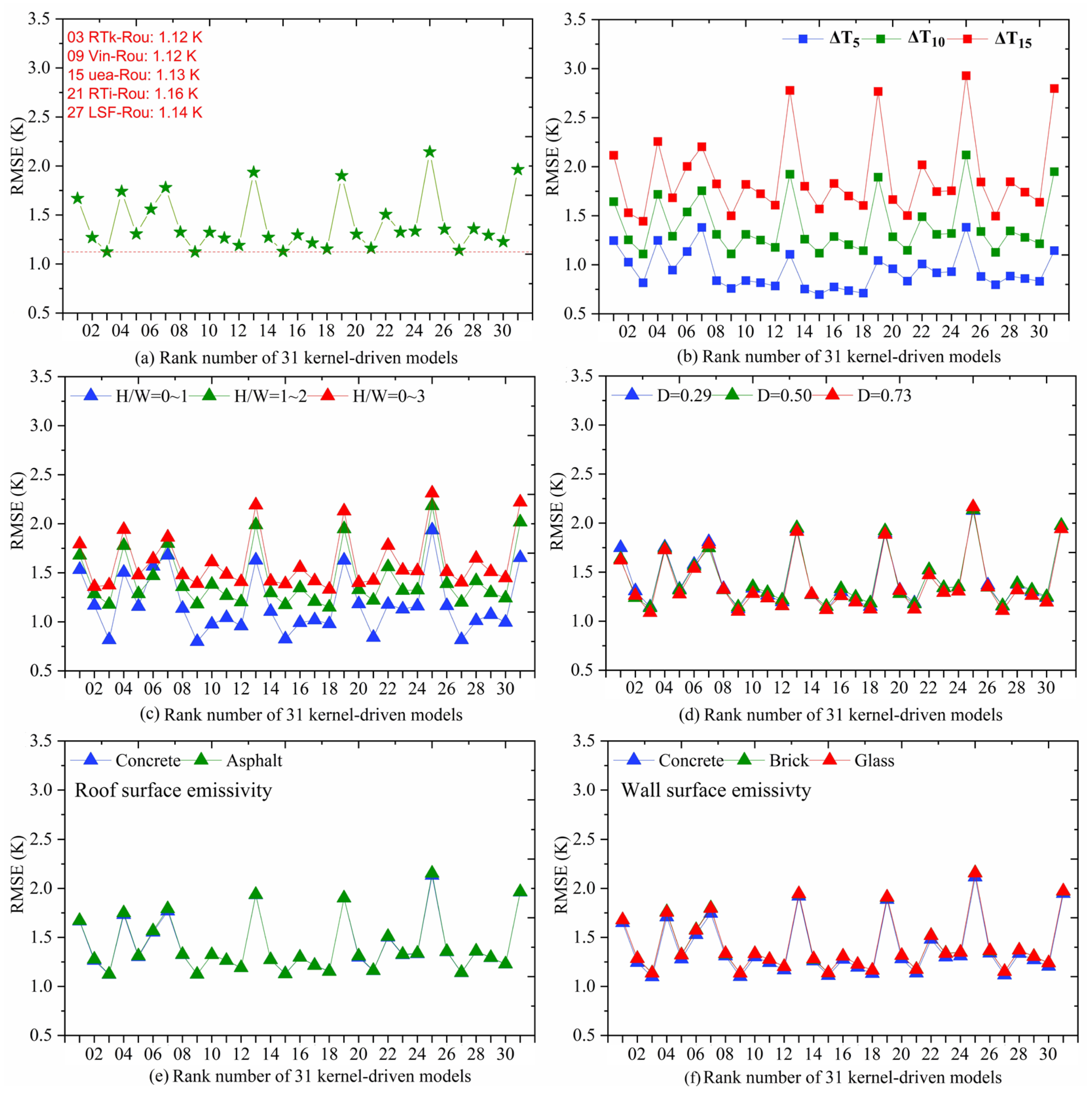
Considering the satellite view angle ranges, the TRD at VZA of 0~60° is selected to compare kernel-driven models (KDMs) and the DART simulation database. In this section, the TRD is operationally defined as the brightness temperature difference between nadir and off-nadir observations to quantitatively evaluate the performance of 31 KDMs. The RL model (01) is a single-kernel model. The other 30 KDMs are dual-kernel models combined with 5 base-shape kernels (RossThick, Vinnikov, uea, RossThin, and LSF) and 6 hotspot kernels (RL, Roujean, Vinnikov, LiSparseR, LiDense, and Chen). Their rank numbers are described in Table 2. As shown in Figure 8a, there is no obvious deviation in performance between the single-kernel-driven and dual-kernel-driven models. The RMSE of the RL single-kernel model is 1.67 K, which outperforms the Chen-series dual-kernel models. The RMSEs of RL-series dual-kernel models (02, 08, 14, 20, 26) are ~1.3 K, and they are superior to the RL single-kernel model. It demonstrates that the incorporation of base-shape kernels can enhance the performance of the hotspot kernel within the same series. Comparing the precision of different hotspot kernel series models, Rou-series dual-kernel models outperform other hotspot-series dual-kernel models, and the overall RMSE is smaller than 1.2 K. The better performance may be due to the underlying theoretical framework of the Roujean KDM, which assumes that the surface objects are long-wall protrusions, and it coincides with realistic urban buildings. The RTk-Rou dual-kernel model (03) and VinB-Rou model (09) have the lowest RMSE of 1.12 K. In addition, the dual-kernel models with the same base-shape kernel are analyzed by different series. KDMs of RTk-series are different from other series, and the performance of the RossThick kernel is not stable with various hotspot kernels. Notably, the VinB-/uea-/LSF-series have similar performance when they are combined with different hotspot kernels. It is probably because the base-shape kernels of the Vinnikov model, the uea model, and the LSF model have a similar function curve. Although the Vinnikov and the uea KDMs are empirically derived, the uea model has slightly superior performance compared to the Vinnikov model, which may be due to its development from the urban simulation database. Chen KDM was deducted based on the physics of radiation interaction with plant canopies, which may lead to poor accuracy of Chen-series dual-kernel models over such urban simulation landscapes. The RMSE of the RTi-Chen dual-kernel model (25) reaches up to 2.14 K. Most KDMs have been developed for vegetation canopies, whose structural assumptions are circular or elliptical crowns and specific leaf area distributions. They differ substantially from the geometric shapes of urban buildings. These discrepancies in geometric representation lead to notable limitations in accurately characterizing hotspots in urban environments. In contrast, the Roujean KDM, which is formulated based on the scattering radiation of long-wall protrusions, exhibits a structural framework more consistent with urban buildings. Therefore, the Rou-series KDMs present the superior performance in these comparisons. These results suggest that the incorporation of realistic urban landscapes is essential for enhancing the performance of KDMs in future research.
To compare the influence of the spectral and geometric parameters on the magnitude between different KDMs and DART TRDs, only one parameter varies within the simulation configurations, whereas the other parameters remain invariant at their settings. The magnitude of RMSE versus component temperature thresholds (ΔT), the ratio between building height and road width (H/W), building densities (D), roof surface emissivity, and wall surface emissivity are also shown in Figure 8. Relevant conclusions can be drawn in Figure 8.
(1)
The magnitude of RMSE increases with the increase in the ΔT from 5 K to 10 K for each KDM, and 31 KDMs are sensitive to various ΔT. The relative magnitude of RMSE in the ΔT is similar to the overall performance for 31 KDMs, but their priority is not completely consistent for each ΔT. The lowest RMSE is 0.70 K for ΔT = 5 K using the uea-Rou dual-kernel model (15). The RTk-Rou dual-kernel model (03) is slightly preferred to other KDMs for ΔT = 10 K and ΔT = 15 K, and its RMSE is 1.11 K and 1.44 K, respectively.
(2)
A total of 31 KDMs are sensitive to various H/W. Except for the RTk-LDR dual-kernel model (06), the magnitude of RMSE increases with the increase in the H/W from 0~1 to 0~3. The RMSE minimum is 0.80 K in the Vin-Rou dual-kernel model, and the overall RMSEs of Rou-series KDMS (09, 03, 27, 15, 21) are always smaller than 0.85 K at H/W = 0~1. The RMSE difference between different H/W is higher than 0.60 K in three Vin-series dual-kernel models (28, 10, 12).
(3)
The RMSEs for 31 KDMs exhibit comparable values in different building densities, consistent with the overall performance. There is no significant difference between 31 KMDs except for the 0.13 K of RL KDMs in different building densities. As observed in Figure 8d, the higher building densities slightly lead to a smaller RMSE. The optimal performance is the RTk-Rou dual-kernel model (03) with an RMSE of 1.09 K in D = 0.73.
(4)
Concrete and asphalt are selected as the building roof material, and their emissivity is 0.893 and 0.928, respectively. As shown in Figure 8e, roof surface emissivity cannot affect the performance of 31 KMDs by more than 0.01 K. In addition, the influence of wall surface emissivity is higher than roof surface emissivity, but their RMSE difference in each KDM is not higher than 0.05 K in Figure 8f. Results indicate that the surface emissivity is not an important parameter for the development of current KMDs when compared with the H/W.
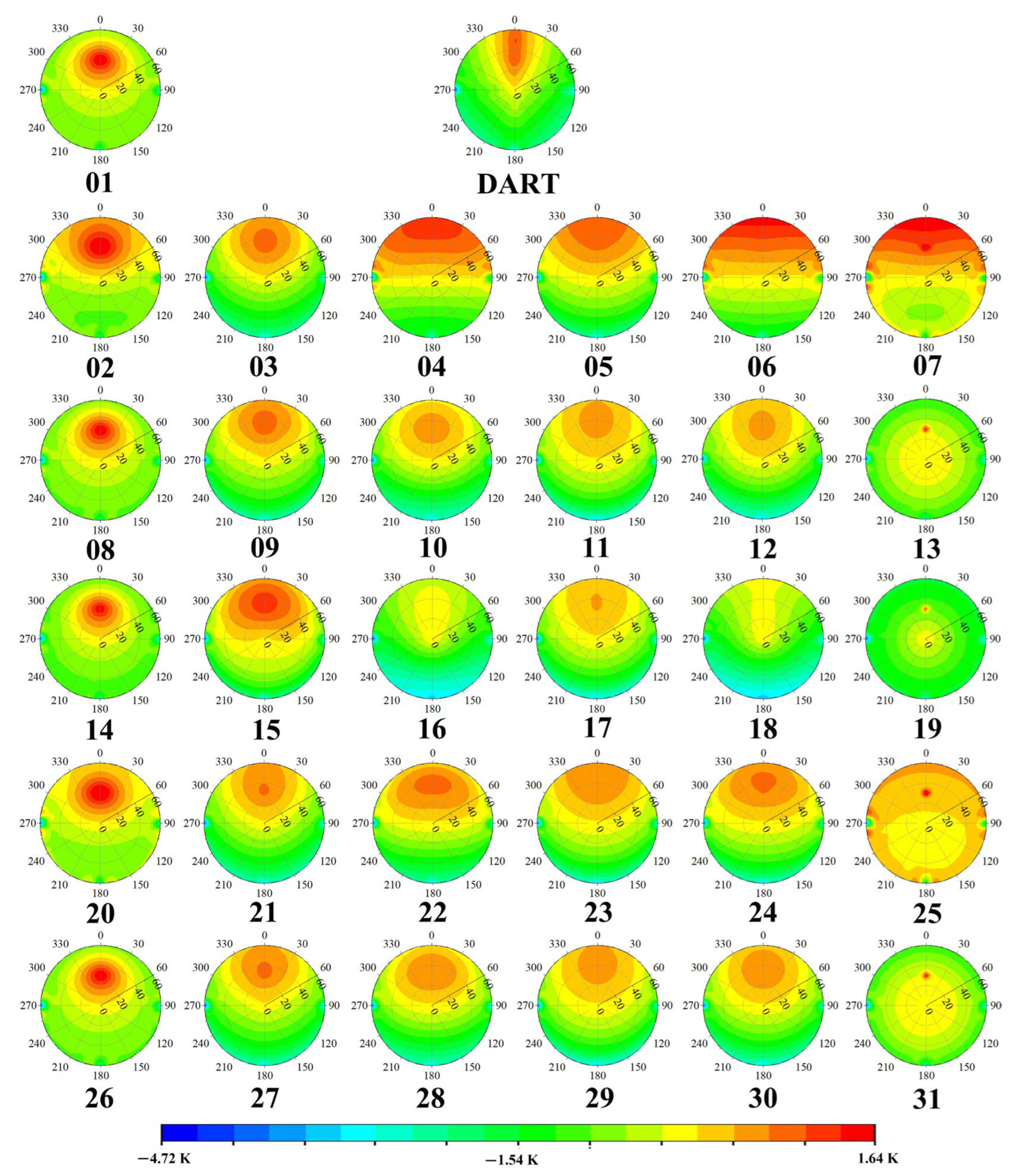
Figure 9 shows the TRD distribution to evaluate the description of hotspots by 31 kernel-driven models. In this case, the component mean temperatures of roofs, walls, and roads are 321 K, 316 K, and 316 K, the component temperature threshold is 5 K, and the building materials of roofs, walls, and roads are asphalt, concrete, and asphalt. The building H/W ranges from 0 to 1, and the building density is 0.29. In DART simulation results, the hotspot location is mainly concentrated in the regions near the solar location, and its shape is narrow and elongated along the main plane of the solar location. In addition, different base-shape kernels lead to significant differences when 31 KDMs are compared with the DART TRD distribution, and the hotspot shapes of the 31 KDMs are all completely different from the DART results. RL-series KDMs have hotspot regions compared to other series of hotspot kernel models, but they describe the hotspot with approximate locations and inconsistent shapes. Rou-series KDMs can simulate a similar shape of the hotspot around the nadir observation, which may lead to their better performance than other KDMs. Conversely, Chen-series KDMs cannot describe the accurate shape of the hotspot, which may be due to the noncircular hotspot shape of the current simulation scenes. Compared with other hotspot-series KDMs, the VinH-/LSR-/LDR-series KDMs have limited ability to describe the hotspot, and their performance relies on the base-shape kernel. The performance of LSR-/LDR-series KDMs is worse than other models, which may be due to their development for different densities of vegetation canopy. Results show that the performance of 31 KDMs mainly depends on the description of the hotspot, and this phenomenon should be considered in the future development of urban KDMs.

4.2.2. The Performance of Kernel-Driven Models at the Solar Plane

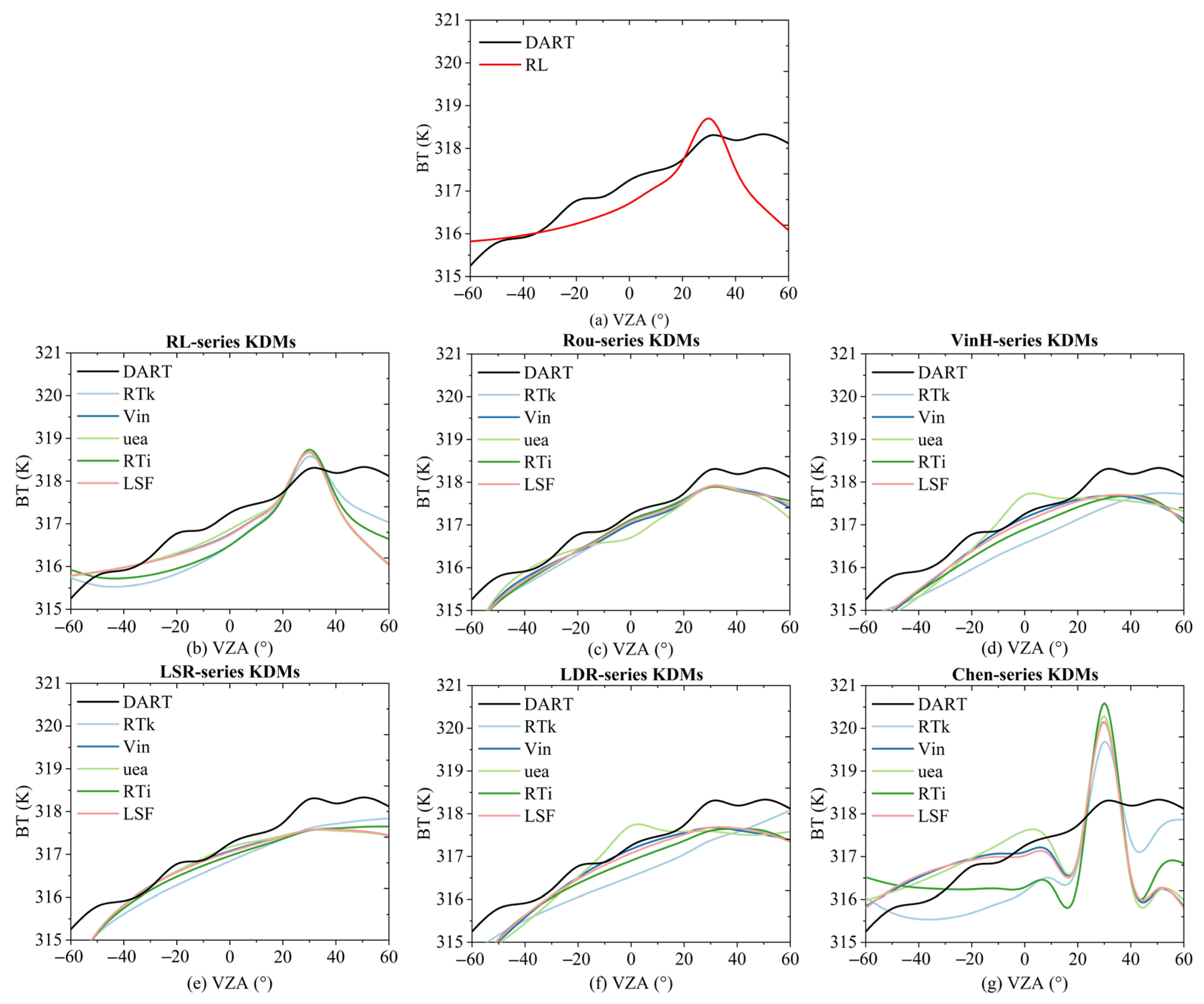
Considering the importance of the hotspot in the TRD study, this study analyzed the TRD performance of 31 KDMs on the solar plane. Figure 10 shows the bias between 31 KDMs and DART DBT results at the solar plane. Compared with DART simulation results, 31 KDMs underestimate the TRD at the solar principal plane (SPP) and overestimate at the cross-solar principal plane (CSPP). At the SPP, the bias of RL-series KDMs (01, 02, 08, 14, 20, 26) is within −1.11 K, and the RL single-kernel model (01) has the lowest bias with −0.71 K. Chen-series KDMs have a similar performance except for the RTk-Chen dual-kernel model (07) with the bias of −1.40 K. The observed similarity between the VinB-series and LSF-series KDMs may be due to the similar function curve of these two single-kernel models. The bias of uea-series KDMs has a consistent distribution, demonstrating that the uea model has a stable performance with different hotspot kernels over urban regions. In addition, the RL-uea dual-kernel model (14) demonstrates superiority at the CSPP in terms of accuracy and variance. The approximation of RossThin single kernel for photon scatters may be unreasonable when it is employed over urban regions, which causes RTi-series KDMs (20~25) to perform significantly worse than the other KDMs both at the SPP and CSPP. In addition, Figure 10 shows that RL KDM (01) can describe the hotspot well at the SPP and cannot obtain better precision at the CSPP, and its difference is due to the absence of the base-shape kernel, demonstrating the importance of the multi-scattering radiation. Similarly, the uea-series present a slight advantage when compared to other KDMs, and it means that the surface geometry shape of target landscapes should be considered in the derivation of KDMs in future studies.
To present a clear comparison between these KDMs, this study divides the KDMs by different hotspot kernels, and the fitted lines for DART and 31 KDM TRD results at the SPP are drawn in Figure 11. DART simulations demonstrate the hotspot phenomenon around the solar location, and the hotspot regions extend to the VZA of 60° in this case. The same hotspot kernel series KDMs have similar fitted lines at the solar plane, except the uea kernel within the VinH-series and LDR-series KDMs. There is an obvious hotspot location in RL-series and Chen-series KDMs around the solar location, and their hotspot regions are concentrated on the VZA of 30°. The DBT distribution trends of other KDMS are similar to the DART results at VZAs from −50° to 30°, but VinH-/LSR-/LDR-series KDMs have an obvious underestimation at the solar plane. VinH-series and LDR-series KDMs have consistent fitted lines before VZA of 50°, and they have a slight difference after VZA of 50°. Rou-series KDMs have a better performance with the same BT trend, and they underestimate the BT at VZAs smaller than −50°. Except for the Chen single-kernel model, other hotspot KDMs have stability in describing the BT at the SPP with different base-shape kernels. In general, the Rou-series KDMs outperform other series KDMs, and most of these KDMs should be optimized by improving the hotspot shapes and regions.

5. Discussion

5.1. The Performance of Multi-Parameter Kernel-Driven Models

Different from the modeling framework of other KDMs from Section 4, GUTA-Sparse and GUTA-Dense models were developed with the inclusion of the “orientation” kernel and the shadow kernel [32,33]. They focus on the importance of component temperature differences in the process of TRD modeling, which is consistent with the theory in the TIR domain. In addition, GUTA-Sparse and GUTA-Dense models outperform in recent TRD studies due to their better performance [38]. Therefore, these two models designed for urban scenarios were selected for comparison between KDMs here.
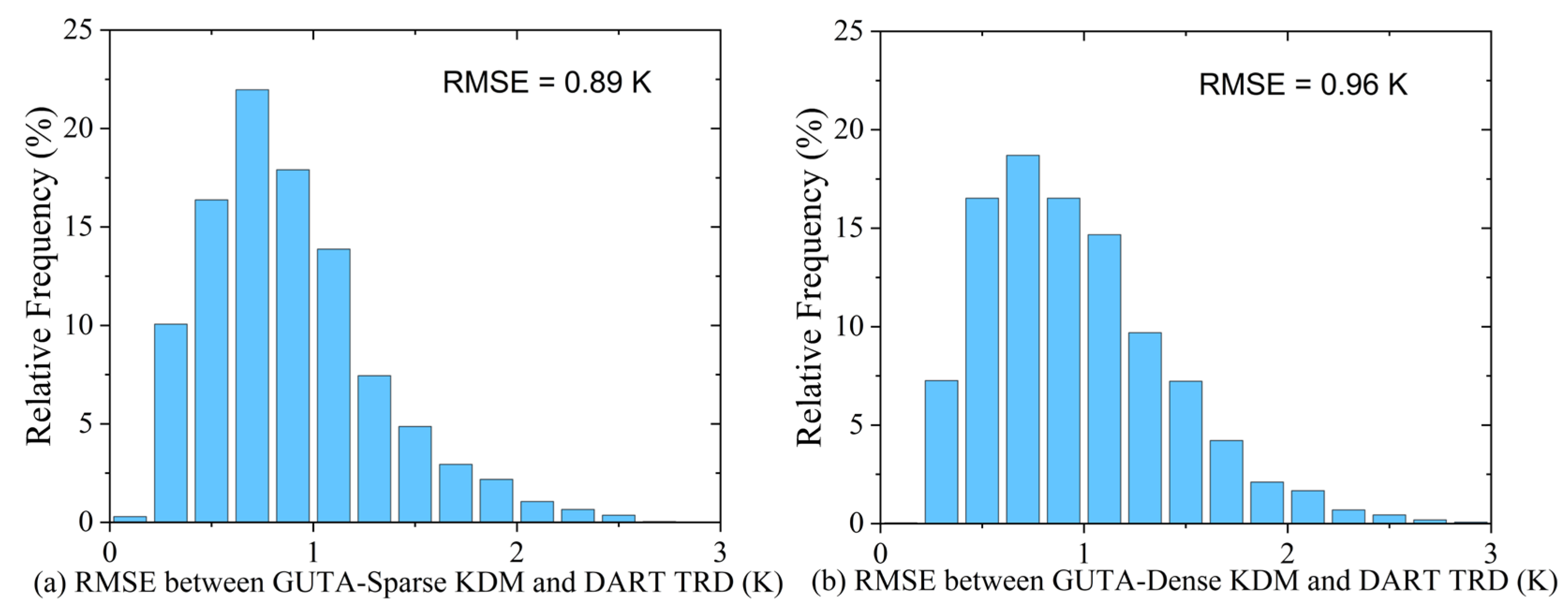
To facilitate the comparison between different KDMs, the same simulation case in Section 4.2.1 is selected for this section. Based on the histograms in Figure 12, the GUTA-Sparse model and the GUTA-Dense model display considerable precision with an overall RMSE of 0.89 K and 0.96 K, which are better than the performance of other KDMs (1.12 K) in Section 4.2.1. Their RMSEs are concentrated on 1.0 K in most simulations, and the performance of the GUTA-Sparse model is superior to the GUTA-Dense model in terms of the TRD statistical values. These improvements may be due to the additional parameters that are considered in GUTA-series models, and the random distribution of buildings can also contribute to the application of Boolean models in this study. In particular, these two models display a limited performance under the simulation scenes with higher H/W and building density, which may be due to the increasing adjacent radiation in such complex scenarios. Given the unsatisfactory descriptions of other KDMs for the hotspot, this study also shows the polar diagrams of GUTA-series models in Figure 13, and the GUTA-Sparse model and the GUTA-Dense model have similar hotspot locations but different hotspot shapes compared to DART results. The TRD polar diagram of the GUTA-Dense model shows better performance than the GUTA-Sparse model, which demonstrates an advantage in describing the shape of hotspots. The simulated scenarios in the GUTA-Sparse/Dense models are derived from the Roujean KDM, whose underlying assumption of long-wall protrusions aligns with the structural characteristics of realistic urban buildings. Their modeling frameworks are physically grounded by explicitly accounting for the sunlit/shadow temperature of component surfaces, as well as the geometric properties of ground structures (building density and H/W). The assumption and framework conform to the radiative transfer theory in the TIR field and enable the GUTA-Sparse/Dense models to surpass other KDMs in performance with one more fitting parameter. In summary, the GUTA-series KDMs display an obvious advantage both in statistical RMSE and spatial distribution of TRD, and the combination of these two models may make them perform better over urban regions.

5.2. Limitations

This study employed the DART simulation database to analyze urban TRD and evaluated the performance of some typical KDMs, and there are some problems to be solved. Firstly, the simulation in DART may be limited, as the realistic urban environments are more complex than the simulation landscapes. They are characterized by many land types, including natural features (vegetation and water bodies) and architecturally irregular built-up structures [5,7,9,61,62]. More solutions should be explored to address the issues of different satellite platforms and high-precision urban surface data to establish a TRD database. It is known that the better performance of TRD models is related to the accurate component temperature and surface emissivity. This study only employed the specific values from airborne data to configure the component temperature and surface emissivity with land covers, whereas they can be influenced by many biophysical parameters. The surface emissivity varies due to the physical condition of materials, and the differences in surface emissivity can cause an LST error of 1–2 K [63]. The LST is a dynamic variable that can be influenced by wind speed, air temperature, and soil moisture [64,65,66]. However, such a dynamic situation is inherently gradual and cannot be achieved in a short period, which is also discussed with the thermal inertia [22]. Therefore, dynamic TRD models should be explored by considering the varying component temperature [11]. In addition, it is undeniable that the atmospheric effect is important in thermal radiation studies, whose accuracy can affect the LST accuracy. The 0.5–2% difference in atmosphere will cause an LST difference of 0.4 K to 1.5 K with different atmospheric humidities [67,68]. Water vapor is the key parameter within the atmosphere, and different atmospheric types should be considered in the derivation of the LST-related studies [69,70]. Finally, all KDMs used in this study can be expressed in the form of standard parameterized models, and other non-linear TRD models were not considered. Future studies would take into account the physical models and the inclusion of the atmosphere to obtain more reasonable TRD results.

6. Conclusions

In this study, the urban TRD database was first generated by the DART models, and the simulation results were employed to analyze the key parameters influencing the urban BTD. In addition, this TRD database is employed to test the performance of 31 classical KDMs, whose sensitivities are also analyzed with surface emissivity, component temperatures, and urban geometric parameters. The major conclusions are as follows:
(1) The band emissivities influence the urban BTD via the influence on BT maximum across the hemispherical domain. The BT minimum cannot vary significantly with the various band emissivities. The BTDs of band emissivities between ECOSTRESS band 3 and band 1 demonstrate an obvious difference, which leads to the biggest ΔBTD of 0.91 K.
(2) The different component temperature thresholds (ΔT) can significantly influence the BTD, which is almost neglected in the previous TRD study. The influence of ΔT increases with the wider temperature ranges, and the RMSE of ΔBTD can reach up to 7.01 K between ΔT15 and ΔT5. Moreover, the magnitude of BTDs exhibits obvious discrepancies between various component temperature differences, and the ΔBTD can be over 10 K. These two parameters jointly emphasize the importance of component temperature.
(3) The H/W and building density can influence the BTD in different aspects. The increasing building density can diminish the urban BTD, whereas the bigger H/W can lead to a higher BTD. However, their influence on the BTD is limited in urban areas. Once their magnitude reaches a particular threshold, the variations cannot further affect the BTD.
(4) The Rou-series dual-kernel models outperform when the available KDMs are compared with the DART TRD, and all of their overall RMSEs are smaller than 1.16 K. These available KDMs are sensitive to the component temperature thresholds and building H/W, and the building density and wall/roof emissivities of simulation scenes cannot affect their performance further.
(5) Most KDMs cannot accurately characterize the hotspot effect over urban regions, neither in terms of the location nor the shapes. The RL single-kernel model performs better with a bias of −0.71 K at the SPP. Based on the same base-shape kernel, the uea-series dual-kernel models display stable superiority both at the SPP and CSPP.
As concluded above, component temperatures play a dominant role in urban BTD analyses and in the performance of available TRD models, and surface emissivity and H/W are also factors influencing urban thermal behavior. In addition, the better performance of these 31 KDMs is due to the balanced error across observation angles, and they cannot completely describe the urban TRD distribution. As we know, the TRD not only compromises the consistency of LST measurements across different observation systems but also increases the complexity of accurately estimating hemispheric radiant exitance. Analyses and comparisons of this study indicate that more TRD models should be developed with these key influencing parameters based on the TIR theory in urban areas, which is beneficial for the study of LST angular normalization and the hemispheric radiative flux evaluation, providing new insights for LST applications.

Author Contributions

Writing—original draft preparation, X.Z.; writing—review and editing, Z.-L.L. and F.N. All authors have read and agreed to the published version of the manuscript.

Funding

This research was funded by the China Scholarship Council (CSC).

Data Availability Statement

The original contributions presented in this study are included in the article. Further inquiries can be directed to the corresponding author.

Acknowledgments

The authors would like to thank the reviewers and the handling editor whose comments and suggestions improved this paper.

Conflicts of Interest

The authors declare no conflicts of interest.

References

  1. Hsu, A.; Sheriff, G.; Chakraborty, T.; Manya, D. Disproportionate exposure to urban heat island intensity across major US cities. Nat. Commun. 2021, 12, 2721. [Google Scholar] [CrossRef] [PubMed]
  2. Imhoff, M.L.; Zhang, P.; Wolfe, R.E.; Bounoua, L. Remote sensing of the urban heat island effect across biomes in the continental USA. Remote Sens. Environ. 2010, 114, 504–513. [Google Scholar] [CrossRef]
  3. Lazzarini, M.; Marpu, P.R.; Ghedira, H. Temperature-land cover interactions: The inversion of urban heat island phenomenon in desert city areas. Remote Sens. Environ. 2013, 130, 136–152. [Google Scholar] [CrossRef]
  4. Rajasekar, U.; Weng, Q. Urban heat island monitoring and analysis using a non-parametric model: A case study of Indianapolis. ISPRS J. Photogramm. Remote Sens. 2009, 64, 86–96. [Google Scholar] [CrossRef]
  5. Ru, C.; Duan, S.-B.; Jiang, X.-G.; Li, Z.-L.; Jiang, Y.Z.; Ren, H.Z.; Leng, P.; Gao, M.F. Land surface temperature retrieval from Landsat 8 thermal infrared data over urban areas considering geometry effect: Method and application. IEEE Trans. Geosci. Remote Sens. 2021, 60, 5000716. [Google Scholar] [CrossRef]
  6. Voogt, J.A.; Oke, T.R. Effects of urban surface geometry on remotely-sensed surface temperature. Int. J. Remote Sens. 1998, 19, 895–920. [Google Scholar] [CrossRef]
  7. Chen, S.S.; Ren, H.Z.; Ye, X.; Dong, J.Q.; Zheng, Y.T. Geometry and adjacency effects in urban land surface temperature retrieval from high-spatial-resolution thermal infrared images. Remote Sens. Environ. 2021, 262, 112518. [Google Scholar] [CrossRef]
  8. Ermida, S.L.; Hulley, G.; Trigo, I.F. Introducing emissivity directionality to the temperature-emissivity separation algorithm. Remote Sens. Environ. 2024, 311, 114280. [Google Scholar] [CrossRef]
  9. Ru, C.; Duan, S.-B.; Jiang, X.-G.; Li, Z.-L.; Huang, C.; Liu, M. An extended SW-TES algorithm for land surface temperature and emissivity retrieval from ECOSTRESS thermal infrared data over urban areas. Remote Sens. Environ. 2023, 290, 113544. [Google Scholar] [CrossRef]
  10. Ouyang, X.Y.; Sun, Z.C.; Zhou, S.G.; Dou, Y.J. Urban land surface temperature retrieval with high-spatial resolution SDGSAT-1 thermal infrared data. Remote Sens. Environ. 2024, 312, 114320. [Google Scholar] [CrossRef]
  11. Cao, B.; Liu, Q.H.; Du, Y.M.; Roujean, J.-L.; Gastellu-Etchegorry, J.-P.; Trigo, I.F.; Zhan, W.F.; Yu, Y.Y.; Cheng, J.; Jacob, F.; et al. A review of earth surface thermal radiation directionality observing and modeling: Historical development, current status and perspectives. Remote Sens. Environ. 2019, 232, 111304. [Google Scholar] [CrossRef]
  12. Fontanilles, G.; Briottet, X.; Fabre, S.; Trémas, T. Thermal infrared radiance simulation with aggregation modeling (TITAN): An infrared radiative transfer model for heterogeneous three-dimensional surface-application over urban regions. Appl. Opt. 2008, 47, 5799–5810. [Google Scholar] [CrossRef] [PubMed]
  13. Lagouarde, J.-P.; Hénon, A.; Kurz, B.; Moreau, P.; Irvine, M.; Voogt, J.; Mestayer, P. Modelling daytime thermal infrared directional anisotropy over Toulouse city centre. Remote Sens. Environ. 2010, 114, 87–105. [Google Scholar] [CrossRef]
  14. Lagouarde, J.-P.; Bach, M.; Sobrino, J.A.; Boulet, G.; Briottet, X.; Cherchali, S.; Coudert, B.; Dadou, I.; Dedieu, G.; Gamet, P.; et al. The MISTIGRI thermal infrared project: Scientific objectives and mission specifications. Int. J. Remote Sens. 2013, 34, 3437–3466. [Google Scholar] [CrossRef]
  15. Zheng, X.P.; Gao, M.F.; Li, Z.-L.; Chen, K.S.; Zhang, X.; Shang, G.F. Impact of 3-D structures and their radiation on thermal infrared measurements in urban areas. IEEE Trans. Geosci. Remote Sens. 2020, 58, 8412–8426. [Google Scholar] [CrossRef]
  16. Zheng, X.P.; Wang, T.X.; Nerry, F.; Guo, Y.Y.; Huang, Z.H. Thermal infrared radiative transfer modeling in urban areas by considering 3-D structures and sunlit-shadow temperature contrast. IEEE Trans. Geosci. Remote Sens. 2023, 61, 5002217. [Google Scholar] [CrossRef]
  17. Duffour, C.; Lagouarde, J.-P.; Roujean, J.-L. A two parameter model to simulate thermal infrared directional effects for remote sensing applications. Remote Sens. Environ. 2016, 186, 250–261. [Google Scholar] [CrossRef]
  18. Lagouarde, J.-P.; Irvine, M. Directional anisotropy in thermal infrared measurements over Toulouse city centre during the CAPITOUL measurement campaigns: First results. Meteorol. Atmos. Phys. 2008, 102, 173–185. [Google Scholar] [CrossRef]
  19. Hu, T.; Du, Y.M.; Cao, B.; Li, H.; Bian, Z.J.; Sun, D.L.; Liu, Q.H. Estimation of upward longwave radiation from vegetation surfaces considering thermal directionality. IEEE Trans. Geosci. Remote Sens. 2016, 54, 6644–6658. [Google Scholar] [CrossRef]
  20. Hu, T.; Roujean, J.-L.; Cao, B.; Mallick, K.; Boulet, G.; Li, H.; Xu, Z.H.; Du, Y.M.; Liu, Q.H. Correction for LST directionality impact on the estimation of surface upwelling longwave radiation over vegetated surfaces at the satellite scale. Remote Sens. Environ. 2023, 295, 113649. [Google Scholar] [CrossRef]
  21. Peng, J.J.; Liu, Q.; Liu, Q.H.; Li, J.H.; Ma, H.Z.; Fang, L. Kernel-driven model fitting of multi-angle thermal infrared brightness temperature and its application. J. Infrared Millim. Waves 2011, 30, 361–365. [Google Scholar] [CrossRef]
  22. Liu, X.Y.; Tang, B.-H.; Li, Z.-L.; Zhang, X.; Shang, G.F. On the derivation of geometric optical kernels for directional thermal radiation. Earth Space Sci. 2020, 7, e2019EA000895. [Google Scholar] [CrossRef]
  23. Cao, B.; Roujean, J.-L.; Gastellu-Etchegorry, J.-P.; Liu, Q.H.; Du, Y.M.; Lagouarde, J.-P.; Huang, H.G.; Li, H.; Bian, Z.J.; Hu, T.; et al. A general framework of kernel-driven modeling in the thermal infrared domain. Remote Sens. Environ. 2021, 252, 112157. [Google Scholar] [CrossRef]
  24. Vinnikov, K.Y.; Yu, Y.Y.; Goldberg, M.D.; Tarpley, D.; Romanov, P.; Laszlo, I.; Chen, M. Angular anisotropy of satellite observations of land surface temperature. Geophys. Res. Lett. 2012, 39, L23802. [Google Scholar] [CrossRef]
  25. Li, X.W.; Strahler, A.H.; Friedl, M.A. A conceptual model for effective directional emissivity from Nonisothermal surfaces. IEEE Trans. Geosci. Remote Sens. 1999, 37, 2508–2517. [Google Scholar] [CrossRef]
  26. Ermida, S.L.; Trigo, I.F.; DaCamara, C.C.; Pires, A. A methodology to simulate LST directional effects based on parametric models and landscape properties. Remote Sens. 2018, 10, 1114. [Google Scholar] [CrossRef]
  27. Ermida, S.L.; Trigo, I.F.; Dacamara, C.C.; Roujean, J.-L. Assessing the potential of parametric models to correct directional effects on local to global remotely sensed LST. Remote Sens. Environ. 2018, 209, 410–422. [Google Scholar] [CrossRef]
  28. Sun, H.; Chen, Y.H.; Zhan, W.F.; Wang, M.J.; Ma, W. A kernel model for urban surface thermal emissivity anisotropy and its uncertainties. J. Infrared Millim. Waves 2015, 34, 66–73. [Google Scholar]
  29. Roujean, J.-L.; Leroy, M.; Deschamps, P.-Y. A bidirectional reflectance model of the earth’s surface for the correction of remote sensing data. J. Geophys. Res. 1992, 97, 20455–20468. [Google Scholar] [CrossRef]
  30. Strahler, A.H.; Jupp, D.L.B. Modeling bidirectional reflectance of forests and woodlands using Boolean models and geometric optics. Remote Sens. Environ. 1990, 34, 153–166. [Google Scholar] [CrossRef]
  31. Wang, D.D.; Chen, Y.H.; Cui, Y.H.; Sun, H. A geometric model to simulate urban thermal anisotropy for simplified neighborhoods. IEEE Trans. Geosci. Remote Sens. 2018, 56, 4930–4944. [Google Scholar] [CrossRef]
  32. Wang, D.D.; Chen, Y.H.; Zhan, W.F. A geometric model to simulate thermal anisotropy over a sparse urban surface (GUTA-sparse). Remote Sens. Environ. 2018, 209, 263–274. [Google Scholar] [CrossRef]
  33. Wang, D.D.; Chen, Y.H. A geometric model to simulate urban thermal anisotropy in simplified dense neighborhoods (GUTA-Dense). IEEE Trans. Geosci. Remote Sens. 2019, 57, 6226–6239. [Google Scholar] [CrossRef]
  34. Bian, Z.J.; Fan, T.Y.; Roujean, J.-L.; Wang, D.D.; Irvine, W.; Wu, S.B.; Cao, B.; Li, H.; Du, Y.M.; Xiao, Q.; et al. An analytical urban temperature model with building heterogeneity using geometric optical theory. Remote Sens. Environ. 2024, 301, 113948. [Google Scholar] [CrossRef]
  35. Ran, X.T.; Cao, B.; Qin, B.X.; Bian, Z.J.; Du, Y.M.; Li, H.; Xiao, Q.; Liu, Q.H. Assessment of five thermal infrared kernel-driven models using limited multiangle observations. IEEE Geosci. Remote Sens. Lett. 2022, 19, 7001605. [Google Scholar] [CrossRef]
  36. Cao, B.; Gastellu-Etchegorry, J.-P.; Du, Y.M.; Li, H.; Bian, Z.J.; Hu, T.; Fan, W.J.; Xiao, Q.; Liu, Q.H. Evaluation of four kernel-driven models in the thermal infrared band. IEEE Trans. Geosci. Remote Sens. 2019, 57, 5456–5475. [Google Scholar] [CrossRef]
  37. Liu, X.Y.; Tang, B.-H.; Li, Z.-L. Evaluation of three parametric models for estimating directional thermal radiation from simulation, airborne, and satellite data. Remote Sens. 2018, 10, 420. [Google Scholar] [CrossRef]
  38. Jiang, L.; Zhan, W.F.; Hu, L.Q.; Huang, F.; Hong, F.L.; Liu, Z.H.; Lai, J.M.; Wang, C.G. Assessment of different kernel-driven models for daytime urban thermal radiation directionality simulation. Remote Sens. Environ. 2021, 263, 112562. [Google Scholar] [CrossRef]
  39. Michel, J.; Hagolle, O.; Hook, S.J.; Roujean, J.-L.; Gamet, P. Quantifying thermal infra-Red directional anisotropy using Master and Landsat-8 simultaneous acquisitions. Remote Sens. Environ. 2023, 297, 113765. [Google Scholar] [CrossRef]
  40. Chang, Y.; Weng, Q.H.; Voogt, J.A.; Xiao, J.F. Urban thermal anisotropies by local climate zones: An assessment using multi-angle land surface temperatures from ECOSTRESS. Remote Sens. Environ. 2025, 322, 114705. [Google Scholar] [CrossRef]
  41. Gastellu-Etchegorry, J.-P. 3D modeling of satellite spectral images, radiation budget and energy budget of urban landscapes. Meteorol. Atmos. Phys. 2008, 102, 187–207. [Google Scholar] [CrossRef]
  42. Gastellu-Etchegorry, J.-P.; Martin, E.; Gascon, F. DART: A 3-D model for simulating satellite images and surface radiation budget. Int. J. Remote Sens. 2004, 25, 73–96. [Google Scholar] [CrossRef]
  43. Wang, Y.J.; Gastellu-Etchegorry, J.-P. DART: Improvement of thermal infrared radiative transfer modeling for simulating top of atmosphere radiance. Remote Sens. Environ. 2020, 251, 112082. [Google Scholar] [CrossRef]
  44. Wang, Y.J.; Gastellu-Etchegorry, J.-P. Accurate and fast simulation of remote sensing images at top of atmosphere with DART-Lux. Remote Sens. Environ. 2021, 256, 112311. [Google Scholar] [CrossRef]
  45. Grau, E.; Durrieu, S.; Fournier, R.; Gastellu-Etchegorry, J.-P.; Yin, T.G. Estimation of 3D vegetation density with Terrestrial Laser Scanning data using voxels. A sensitivity analysis of influencing parameters. Remote Sens. Environ. 2017, 191, 373–388. [Google Scholar] [CrossRef]
  46. Qin, B.X.; Cao, B.; Roujean, J.-L.; Gastellu-Etchegorry, J.-P.; Bian, Z.J.; Du, Y.M.; Hu, T.; Xiao, Q.; Chen, S.S.; Liu, Q.H. A thermal radiation directionality correction method for the surface upward longwave radiation of geostationary satellite based on a time-evolving kernel-driven model. Remote Sens. Environ. 2023, 294, 113599. [Google Scholar] [CrossRef]
  47. Oltra-Carrio, R.; Cubero-Castan, M.; Briottet, X.; Sobrino, J.A. Analysis of the performance of the TES algorithm over urban areas. IEEE Trans. Geosci. Remote Sens. 2014, 52, 6989–6998. [Google Scholar] [CrossRef]
  48. Sobrino, J.A.; Oltra-Carró, R.; Jiménez-Muñoz, J.C.; Julien, Y.; Sòria, G.; Franch, B.; Mattar, C. Emissivity mapping over urban areas using a classification-based approach: Application to the Dual-use European Security IR Experiment (DESIREX). Int. J. Appl. Earth Obs. Geoinf. 2012, 18, 141–147. [Google Scholar] [CrossRef]
  49. Sobrino, J.A.; Oltra-Carró, R.; Sòria, G.; Jiménez-Muñoz, J.C.; Franch, B.; Hidalgo, V.; Mattar, C.; Julien, Y.; Cuenca, J.; Romaguera, M.; et al. Evaluation of the surface urban heat island effect in the city of Madrid by thermal remote sensing. Int. J. Remote Sens. 2013, 34, 3177–3192. [Google Scholar] [CrossRef]
  50. Li, Z.-L.; Wu, H.; Duan, S.-B.; Zhao, W.; Ren, H.Z.; Liu, X.Y.; Leng, P.; Tang, R.L.; Ye, X.; Zhu, J.S.; et al. Satellite remote sensing of global land surface temperature: Definition, methods, products, and applications. Rev. Geophys. 2023, 61, e2022RG000777. [Google Scholar] [CrossRef]
  51. Meerdink, S.K.; Hook, S.J.; Roberts, D.A.; Abbott, E.A. The ECOSTRESS spectral library version 1.0. Remote Sens. Environ. 2019, 230, 111196. [Google Scholar] [CrossRef]
  52. Zheng, X.P.; Guo, Y.Y.; Zhou, Z.L.; Wang, T.X. Improvements in land surface temperature and emissivity retrieval from Landsat-9 thermal infrared data. Remote Sens. Environ. 2024, 315, 114471. [Google Scholar] [CrossRef]
  53. Morrison, W.; Grimmond, S.; Kotthaus, S. Simulating satellite urban land surface temperatures: Sensitivity to sensor view angle and assumed landscape complexity. Remote Sens. Environ. 2023, 293, 113579. [Google Scholar] [CrossRef]
  54. Egbert, D.D. A practical method for correcting bidirectional reflectance variations. In Proceedings of the machine processing of remotely sensed data symposium, West Lafayette, IN, USA, 21–23 June 1977; pp. 178–189. [Google Scholar]
  55. Wanner, W.; Li, X.; Strahler, A.H. On the derivation of kernels for kernel-driven models of bidirectional reflectance. J. Geophys. Res. 1995, 100, 21077–21089. [Google Scholar] [CrossRef]
  56. Ross, J.L. The Radiation Regime and Architecture of Plant Stands; Springer: Dordrecht, The Netherlands, 1981. [Google Scholar] [CrossRef]
  57. Roujean, J.-L. A parametric hot spot model for optical remote sensing applications. Remote Sens. Environ. 2000, 71, 197–206. [Google Scholar] [CrossRef]
  58. Li, X.W.; Strahler, A.H. Geometric-Optical bidirectional reflectance modeling of discrete crown vegetation canopy: Effect of crown shape and mutual shadowing. IEEE Trans. Geosci. Remote Sens. 1992, 30, 276–292. [Google Scholar] [CrossRef]
  59. Li, X.W.; Strahler, A.H. Geometric-Optical bidirectional reflectance modeling of a conifer forest canopy. IEEE Trans. Geosci. Remote Sens. 1986, 24, 906–919. [Google Scholar] [CrossRef]
  60. Chen, J.M.; Cihlar, J. A hotspot function in a simple bidirectional reflectance model for satellite applications. J. Geophys. Res. 1997, 102, 25907–25913. [Google Scholar] [CrossRef]
  61. Oltra-Carrio, R.; Sobrino, J.A.; Franch, B.; Nerry, F. Land surface emissivity retrieval from airborne sensor over urban areas. Remote Sens. Environ. 2012, 123, 298–305. [Google Scholar] [CrossRef]
  62. Wang, D.D.; Chen, Y.H.; Hu, L.Q.; Voogt, J.A.; He, X.Y. Satellite-based daytime urban thermal anisotropy: A comparison of 25 global cities. Remote Sens. Environ. 2022, 283, 113312. [Google Scholar] [CrossRef]
  63. Li, Z.-L.; Tang, B.-H.; Wu, H.; Ren, H.Z.; Yan, G.J.; Wan, Z.M.; Trigo, I.F.; Sobrino, J.A. Satellite-derived land surface temperature: Current status and perspectives. Remote Sens. Environ. 2013, 131, 14–37. [Google Scholar] [CrossRef]
  64. Lai, S.X.; Zhao, Y.J.; Fan, Y.F.; Ge, J. Characteristics of daytime land surface temperature in wind corridor: A case study of a hot summer and warm winter city. J. Build. Eng. 2021, 44, 103370. [Google Scholar] [CrossRef]
  65. Nascimento, A.C.L.; Galvani, E.; Gobo, J.P.A.; Wollmann, C.A. Comparison between air temperature and land surface temperature for the City of São Paulo, Brazil. Remote Sens. 2022, 13, 491. [Google Scholar] [CrossRef]
  66. Weiland, L.; Rogers, C.A.; Sothe, C.; Arain, M.A.; Gonsamo, A. Satellite-based land surface temperature and soil moisture observations accurately predict soil respiration in temperate deciduous and coniferous forests. Agric. For. Meteorol. 2023, 340, 109618. [Google Scholar] [CrossRef]
  67. Dash, P.; Göttsche, F.M.; Olesen, F.S.; Fischer, H. Land surface temperature and emissivity estimation from passive sensor data: Theory and practice-current trends. Int. J. Remote Sens. 2002, 23, 2563–2594. [Google Scholar] [CrossRef]
  68. Wan, Z.M. MODIS Land-Surface Temperature Algorithm Theoretical Basis Document (LST ATBD); NASA/GSFC: Greenbelt, MD, USA, 1999; pp. 1–77.
  69. Feng, J.-L.; Cai, X.-M.; Chapman, L. Impact of atmospheric conditions and levels of urbanization on the relationship between nocturnal surface and urban canopy heat islands. Q. J. R. Meteorol. Soc. 2019, 145, 3284–3299. [Google Scholar] [CrossRef]
  70. Huang, F.; Zhan, W.F.; Wang, Z.-H.; Voogt, J.; Hu, L.Q.; Quan, J.L.; Liu, C.; Zhang, N.; Lai, J.M. Satellite identification of atmospheric-surface-subsurface urban heat islands under clear sky. Remote Sens. Environ. 2020, 250, 112039. [Google Scholar] [CrossRef]
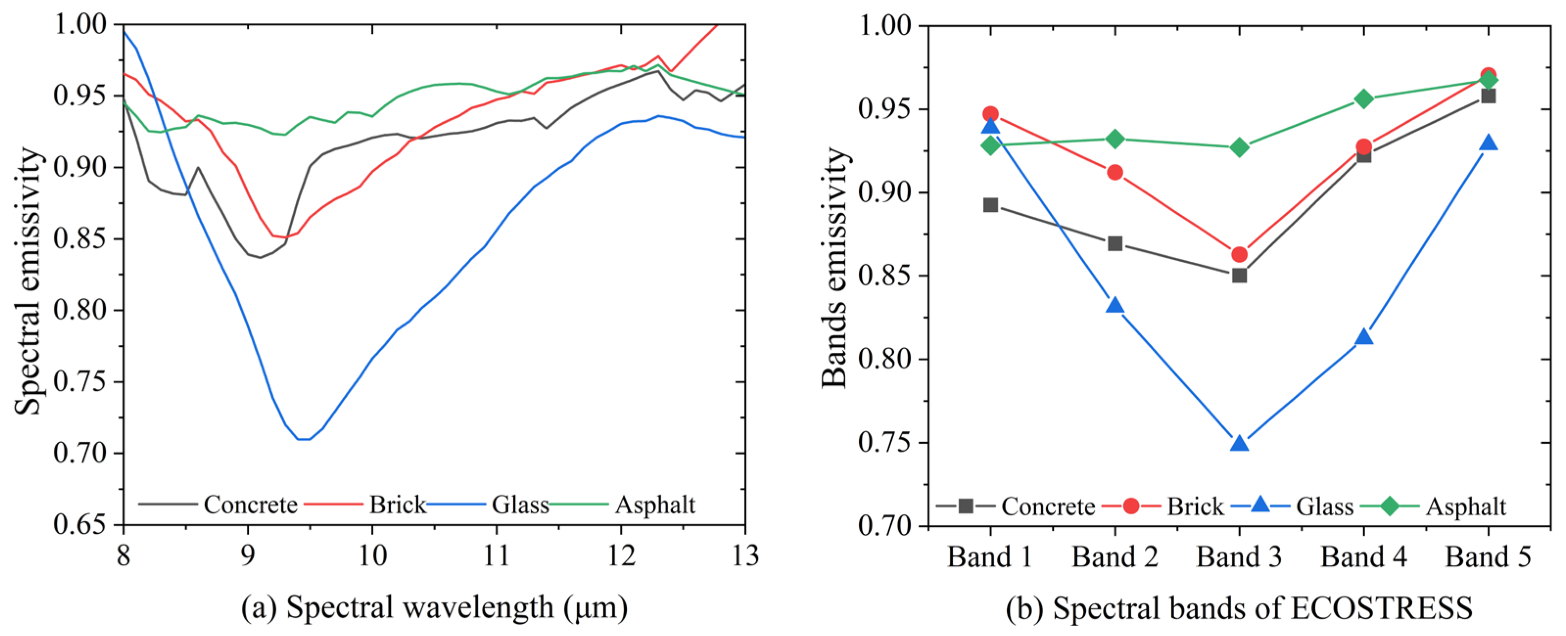
Figure 1. (a) The spectral emissivity for asphalt, concrete, brick, and glass from the ECOSTRESS dataset; (b) the ECOSTRESS band emissivities for asphalt, concrete, brick, and glass.
Remotesensing 17 02884 g001
Figure 2. Diagram of the simulation building scenarios for DART and the 3D visualization of the simulation scene. Each subdiagram represents an ECOSTRESS pixel scenario with different building heights (described in the color bar) and densities, and the blank spaces within each subdiagram represent urban ground (including roads of 5 m width). Based on building heights/road widths (H/W) and building densities (D), each building scenario is abbreviated as (a) S1 (H/W = 0~1, D = 0.29), (b) S2 (H/W = 0~1, D = 0.50), (c) S3 (H/W = 0~1, D = 0.73), (d) S4 (H/W = 1~2, D = 0.29), (e) S5 (H/W = 1~2, D = 0.50), (f) S6 (H/W = 1~2, D = 0.73), (g) S7 (H/W = 0~3, D = 0.29), (h) S8 (H/W = 0~3, D = 0.50), (i) S9 (H/W = 0~3, D = 0.73), and (j) the 3D visualization of (a) S1.
Remotesensing 17 02884 g002
Figure 3. Flowchart of DART database generation, the analysis of urban brightness temperature maximum–minimum discrepancies (BTD = BTmax − BTmin), and the accuracy assessment of 31 kernel-driven models (KDMs).
Remotesensing 17 02884 g003
Figure 4. The BT maximum and BT minimum of all simulation scenes across the hemispherical domain. (a) The BT maximum of simulation scenes for band 1 (black line) and the BT maximum discrepancy (BTAD) between other bands and band 1, (b) the BT minimum of simulation scenes for band 1 (black line) and the BT minimum discrepancy (BTID) between other bands and band 1, and (c) the BTD (BTD = BTmax − BTmin) scatterplots of ECOSTRESS bands.
Remotesensing 17 02884 g004
Figure 5. Histogram of BTD discrepancy (ΔBTD) between different component temperature thresholds (ΔT) in ECOSTRESS band 1. (a) The ΔBTD between 10 K component temperature thresholds (ΔT10) and 5 K component temperature thresholds (ΔT5), and (b) the ΔBTD between 15 K component temperature thresholds ΔT15 and ΔT5.
Remotesensing 17 02884 g005
Figure 6. Diagram of the average BTD in different urban simulation building scenes across the hemispherical domain.
Remotesensing 17 02884 g006
Figure 7. BTD quartile distribution in different component temperature differences across the hemispherical domain, and the red points are the mean value of each group.
Remotesensing 17 02884 g007
Figure 8. RMSEs between 31 kernel-driven models (KDMs) and DART simulation TRDs at VZA of 0~60°, and the rank number is described in Table 2. (a) The overall RMSEs between 31 KDMs and DART TRDs, and the red dashed line is the location of the RMSE minimum. RMSEs between 31 KDMs and DART TRDs in (b) the component temperature threshold, (c) the H/W, (d) the building density, (e) the roof surface emissivity, and (f) the wall surface emissivity.
Remotesensing 17 02884 g008
Figure 9. Polar diagrams of DART simulation and 31 KDM TRDs at VZA of 0~60° in the case of asphalt roofs (321 K) and roads (316 K), concrete walls (316 K), H/W = 0~1, D = 0.29, and ΔT = 5 K. “DART” is the DART simulation TRD, “01” is RL KDM TRD, other rank numbers described in Table 2, the polar diagrams of horizontal rows are the TRD of the same base-shape kernel with varying hotspot kernel, and the polar diagrams of vertical columns are the TRD of the same hotspot kernel with varying base-shape kernels.
Remotesensing 17 02884 g009
Figure 10. Quartile box diagrams of the performance between 31 KDMs and DART TRDs at (a) the solar principal plane (SPP) and (b) the cross-solar principal plane (CSPP).
Remotesensing 17 02884 g010
Figure 11. Diagrams of DART and 31 KDMs BT fitted lines in the solar principal plane (SPP).
Remotesensing 17 02884 g011
Figure 12. Histograms of RMSE between GUTA-Sparse/Dense multi-parameter KDMs and DART TRD.
Remotesensing 17 02884 g012
Figure 13. Polar diagrams of (a) DART model, (b) GUTA-Sparse model, and (c) GUTA-Dense model TRD results at VZA of 0~60° in the case of asphalt roofs (321 K) and roads (316 K), concrete walls (316 K), H/W = 0~1, D = 0.29, and ΔT = 5 K.
Remotesensing 17 02884 g013
Table 1. Description of parameter settings within simulation scenarios.
TypeDescriptionParameter Setting2592
SizeSimulation scene70 m × 70 m (0.5 m × 0.5 m × 0.5 m)
WavelengthECOSTRESS8.29 µm, 8.78 µm, 9.20 µm, 10.49 µm, 12.09 µm
Solar angleZenith angle30°
Azimuth angle
View angle
(310 directions)
Zenith angle0~86°
Azimuth angle0~360°
RoofsOptical propertiesConcreteAsphalt 2
Surface temperatureTroof + 5 KTroof − 5 KTroof − 10 KTroof − 20 K4
WallsOptical propertiesConcreteBrickGlass 3
Surface temperatureTroof = 321 K ± 5 K, ±10 K, ±15 K3
RoadsOptical propertiesAsphalt 1
Surface temperatureTroof + 5 KTroof − 5 KTroof − 10 KTroof − 20 K4
Building densitySroofs/Stotal0.290.500.73 3
Geometry factorH/W0–1/0.51–2/1.50–3/1.5 3
Note: A total of 162 cases are also included with the same average component temperature (321 K) to analyze the influence of temperature difference.
Table 2. The ranking number of KDMs with base-shape kernels and hotspot kernels.
RLRouVinHLSRLDRChen
/01
RTk020304050607
VinB080910111213
uea141516171819
RTi202122232425
LSF262728293031
Table 3. Groups of component temperature differences (Troof = 321 K, δT1 = TroofTwall, δT2 = TroofTroad).
T01T02T03T04T05T06T07T08T09
δT1 (K)0−551020−5−5−55
δT2 (K)0−55102051020−5
T10T11T12T13T14T15T16T17
δT1 (K)55101010202020
δT2 (K)1020−5520−5510
Disclaimer/Publisher’s Note: The statements, opinions and data contained in all publications are solely those of the individual author(s) and contributor(s) and not of MDPI and/or the editor(s). MDPI and/or the editor(s) disclaim responsibility for any injury to people or property resulting from any ideas, methods, instructions or products referred to in the content.