Article

Wind Field Retrieval from Fengyun-3E Radar Based on a Backpropagation Neural Network

1
Collaborative Innovation Center on Forecast and Evaluation of Meteorological Disasters, CMA Key Laboratory for Aerosol-Cloud-Precipitation, Nanjing University of Information Science & Technology, Nanjing 210044, China
2
School of Atmospheric Physics, Nanjing University of Information Science & Technology, Nanjing 210044, China
3
Guangxi Meteorological Observatory, Nanning 530022, China
4
Department of Geography, Harokopio University of Athens, EI. Venizelou 70, Kallithea, 17671 Athens, Greece
5
Aerospace Information Research Institute, Chinese Academy of Sciences, Beijing 100101, China
6
Key Laboratory of Radiometric Calibration and Validation for Environmental Satellites, National Satellite Meteorological Center (National Center for Space Weather), China Meteorological Administration, Beijing 100081, China
7
School of Atmospheric Sciences, Nanjing University of Information Science & Technology, Nanjing 210044, China
*
Author to whom correspondence should be addressed.
Remote Sens. 2025, 17(16), 2813; https://doi.org/10.3390/rs17162813
Submission received: 24 May 2025 / Revised: 27 July 2025 / Accepted: 5 August 2025 / Published: 14 August 2025

Abstract

Ocean surface wind fields are crucial for marine environmental research and applications in weather forecasting, ocean disaster monitoring, and climate change studies. However, traditional wind retrieval methods often struggle with modeling complexity and ambiguity due to the nonlinear nature of geophysical model functions (GMFs), leading to increased computational costs and reduced accuracy. To tackle these challenges, this study establishes a sea surface wind field retrieval model employing a backpropagation (BP) neural network, which integrates multi-angular observations from the Wind Radar (WindRAD) sensor aboard the Fengyun-3E (FY-3E) satellite. Experimental results show that the proposed model achieves high precision in retrieving both wind speed and direction. The wind speed model achieves a root-mean-square error (RMSE) of 1.20 m/s for the training set and 1.00 m/s for the selected test set when using ERA5 data as the reference, outperforming the official WindRAD products. For wind direction, the model attains an RMSE of 23.99° on the training set and 24.58° on the test set. Independent validation using Tropical Atmosphere Ocean (TAO) buoy observations further confirms the model’s effectiveness, yielding an RMSE of 1.29 m/s for wind speed and 24.37° for wind direction, also surpassing official WindRAD products. The BP neural network effectively captures the nonlinear relationship between wind parameters and radar backscatter signals, showing significant advantages over traditional methods and maintaining good performance across different wind speeds, particularly in the moderate range (4–10 m/s). In summary, the method proposed herein significantly enhances wind field retrieval accuracy from space; it has the potential to optimize satellite wind field products and improve global wind monitoring and meteorological forecasting.

1. Introduction

As a fundamental element influencing marine systems, the sea surface wind field is of vital importance in oceanographic research. It directly drives sea surface waves, influencing significant wave height (SWH) and wave age, thereby regulating coastal wave setup. Variations in the wind field not only control local wave trends but also indirectly affect sea conditions in other areas by remotely generating aged waves [1,2]. Moreover, understanding the spatiotemporal evolution characteristics of sea surface wind fields is of great scientific and practical significance for assessing future disaster exposure in coastal areas and making disaster prevention decisions. Therefore, investigating sea surface wind patterns contributes significantly to analyzing ocean dynamics and offers critical support in tracking climate trends, carbon exchange processes, and changes in marine ecological systems.
Satellite remote sensing, with its advantages of wide coverage and high timeliness, provides more accurate and comprehensive sea surface wind field data. Among them, satellite-borne microwave scatterometers are widely used remote sensing instruments, offering all-weather, day-and-night observation capabilities to continuously provide high-quality wind field information [3,4]. Launched by NASA (National Aeronautics and Space Administration) in 1978, Seasat-A was one of the earliest satellites dedicated to ocean remote sensing. Demonstrations from its spaceborne scatterometer (Seasat-A Scatterometer, SASS) validated the capability of satellite microwave scatterometers in retrieving sea surface wind information [5,6]. At present, scatterometer-derived wind field data have been widely applied in oceanographic studies, including weather monitoring, cyclone detection and tracking, hurricane surveillance, air–sea interaction analysis, and climatology research, showcasing their significant value in investigating ocean dynamics and climate systems [7].
Although the technical feasibility of scatterometer-based sea surface wind retrieval has been well verified, due to their working principle, these instruments measure backscattered echo signals rather than direct wind speed and direction. This indirect measurement necessitates the use of specific retrieval algorithms to convert scattering signals into usable wind field parameters. Nevertheless, interpreting radar backscatter in terms of the wind field is complicated by multiple factors, including wind velocity, evolving surface roughness, short-wave dynamics, and other air–sea coupling mechanisms. Additionally, the response of backscatter to wind direction depends on the state of the atmospheric boundary layer [8], making the wind retrieval process quite challenging. To tackle this nonlinear mapping, various algorithms employ different modeling approaches, resulting in differences in retrieval accuracy. Currently, most conventional methods rely on GMFs, which are derived from observational data and serve to estimate wind speed and direction based on backscatter measurements [9]. However, due to idealized assumptions about boundary layer wind profiles in existing models, which often diverge from reality under varying atmospheric stability, these models face limitations in accurately capturing electromagnetic interactions with the sea surface [10]. As a result, operational GMFs are typically constructed using statistical methods or region-specific adaptations to improve retrieval accuracy. In practice, Maximum Likelihood Estimation (MLE) algorithms achieve joint determination of wind speed with direction by formulating and then maximizing a likelihood function [11,12].
Nevertheless, GMF-based retrievals are not unique and often suffer from directional ambiguity, significantly affecting wind direction accuracy [13]. To address this, many scholars have proposed improved ambiguity resolution strategies. For example, in 1999, using data from NSCAT (NASA Scatterometer), Wentz et al. [14] developed the NSCAT-1 model, which performed stably for wind direction and low wind speed retrieval but tended to underestimate wind speeds under strong wind conditions, such as those associated with hurricanes. Later, researchers proposed enhanced models such as NSCAT-5 by Wang et al. [15], which improved upon the Ku-band NSCAT-4 GMF by refining the dependency of backscatter on wind speed and direction and incorporating sea surface temperature (SST), making it suitable for wind retrieval from the HaiYang-2 (HY-2) satellite’s scatterometer. This model effectively removed SST-related wind retrieval bias and no longer showed pronounced meridional patterns. Yang et al. [16] used the HY-2B scatterometer (HSCAT-B) scatterometer data to apply both NSCAT-4 and NSCAT-5 GMFs and introduced stress-equivalent winds and equivalent-neutral winds as improved buoy reference winds, enhancing model accuracy by selecting different reference types according to regional characteristics. Beyond the NSCAT series, many researchers have explored new wind retrieval models. To retrieve wind vectors under precipitation, Liu et al. [17] constructed a hybrid model utilizing data from HY-2B’s scatterometer and radiometer. The 6.925 GHz polarization ratio (PR06) of brightness temperature was adopted as a rainfall-sensitive parameter, followed by statistical regression to estimate wind speed. To retrieve wind direction, a new GMF that accounts for the influence of rainfall was constructed. Experimental results under precipitation conditions showed retrieval deviations of approximately 1.60 m/s for wind velocity and 20.60° for wind azimuth, though performance degraded slightly with increasing rain rate. Li et al. [18] incorporated altimeter backscatter into the wind retrieval process, building empirical GMFs to relate C-band and Ku-band altimeter backscatter with 10 m neutral winds. Combined with MLE, this approach enabled joint retrieval from both scatterometer and altimeter data, improving retrieval accuracy in nadir regions for HY-2B, though results in other regions showed no significant improvement.
Overall, while satellite-borne microwave scatterometer wind retrieval techniques have made significant progress and are widely applied, algorithm adaptability across different scatterometer types remains limited. Most retrievals also rely on additional ambiguity resolution steps, increasing computational cost and model complexity. Therefore, evidently there is still room for optimizing both the accuracy and efficiency of the wind retrieval methods currently employed.
As a critical component of China’s upgraded polar-orbiting meteorological satellite system, FengYun-3E (FY-3E) pioneers the implementation of a morning-evening terminator orbit, enhancing diurnal monitoring continuity [19]. It continues conventional global imaging and atmospheric sounding tasks, with a stronger focus on numerical weather prediction. It has significant advantages in weather forecasting, tropical cyclone and extreme weather warnings, climate change monitoring, and space weather observations. FY-3E carries the Wind Radar (WindRAD) scatterometer, designed to continuously monitor global wind vectors (speed and direction) with high precision and resolution under all-weather and all-time conditions. It also supports inversion of sea ice classification [20], soil moisture, and other surface parameters, enhancing remote sensing capabilities in air–sea interaction studies.
In 2023, He et al. [21] applied the CMOD5.N GMF, combined with the MLE approach and the two-dimensional variational (2DVAR) method, to retrieve sea surface wind fields from Level-1 FY-3E WindRAD observations. Results showed a standard deviation of 1.45 m/s between inversion and measured wind speed, indicating generally good accuracy. However, large deviations remained in some regions, and due to the presence of directional ambiguities, wind direction retrieval showed low accuracy, with average errors exceeding 20°. Therefore, further improvement is needed in spatial consistency and retrieval precision. In this context, this research introduces a novel approach for wind field estimation utilizing the Backpropagation (BP) neural network. In this framework, artificial neural networks are capable of capturing latent relationships from historical data and building models that adaptively adjust parameters to suit different scenarios. Compared to conventional physical or empirical techniques, neural models demonstrate enhanced adaptability and accuracy, allowing for effective handling of complex prediction tasks [22].
In light of the above discussion, the objective of this study is to mitigate the ambiguity problem in wind direction and increase the reliability of sea surface wind inversion results by fully exploring the nonlinear relationship between satellite microwave scatterometer observations and wind speed and direction. Based on the BP neural network algorithm, a novel wind field retrieval method is proposed by integrating FY-3E satellite WindRAD observations with ECMWF Reanalysis v5 (ERA5) data. The key innovation of this study lies in the first application of artificial neural networks to the wind field retrieval modeling using FY-3E WindRAD data, effectively addressing the long-standing directional ambiguity problem encountered by traditional retrieval models such as GMFs. Furthermore, this study takes advantage of the multi-angular observation capability of WindRAD by integrating information from four distinct viewing geometries, which significantly leads to more accurate and consistent results of wind field retrieval. In summary, this article aims to construct a methodology that offers higher precision and robustness for retrieving sea surface wind fields, thereby improving the reliability and performance of wind field inversion based on FY-3E WindRAD observations.

2. Materials and Methods

2.1. FY-3E Data

FY-3E, launched in July 2021, is the first satellite operating in a dawn–dusk sun-synchronous orbit within China’s new-generation weather satellite series. It fills a critical gap in the worldwide satellite-based weather monitoring network for this orbit. Operating in coordination with the morning-orbit satellites (FY-3C/D) and the afternoon-orbit satellite (FY-3D), FY-3E enables global coverage of meteorological observations every six hours, significantly facilitating timely and high-fidelity numerical weather predictions.
FY-3E is equipped with WindRad, the first active microwave remote sensing payload aboard the FengYun satellite series. WindRad commenced normal operations on 9 July 2021. The primary mission of WindRad is to provide all-weather, all-day, and high-accuracy measurements of global sea surface wind vectors (speed and direction). These observations serve as critical inputs for data assimilation in NWP models and support weather forecasting services. In addition, WindRad is also capable of detecting surface features such as sea ice, snow cover, and soil conditions, thereby expanding its applications in Earth environment monitoring. It is a dual-frequency, dual-polarization radar system utilizing a conical scanning strategy with a fan-beam antenna pattern [23]. The radar system operates at both the C-band (5.4 GHz) and Ku-band (13.256 GHz). Since the beamwidth is approximately proportional to the wavelength, the C-band exhibits a wider beamwidth in the range direction compared to the Ku-band, resulting in broader echo returns. To avoid overlap between successive echoes, the C-band adopts a longer pulse repetition interval (PRI) than the Ku-band. Specifically, during scanning, the Ku-band employs a pulse width of 1.7 ms and a PRI of 4.8 ms, whereas the C-band uses a pulse width of 1.8 ms and a PRI of 9.6 ms. Observations in the two frequency bands are conducted independently. In terms of spatial resolution, the azimuth resolution is approximately 25 km for the C-band and 10 km for the Ku-band, while the range resolution is better than 0.5 km for both bands. Each frequency band supports two polarization modes—horizontal (HH) and vertical (VV). The radar antenna performs a full 360° rotation at an angular velocity of 0.6 rad/s, enabling WindRad to acquire a rich set of multi-frequency and multi-polarization backscatter measurements. This design significantly enhances the system’s capability to adapt to various observational scenarios and complex meteorological conditions [24]. The technical specifications of WindRad are summarized in
Table 1, and its observation strategy is illustrated in Figure 1.
This study primarily utilizes Level-1 Ku-band and C-band data (including both HH and VV polarizations), as well as Level-2 ocean surface wind vector orbit products, obtained from both ascending and descending passes of the spaceborne WindRAD instrument onboard the FY-3E satellite. To ensure the representativeness of the dataset and to capture a broad range of wind speed and direction variations, this study utilizes data spanning two years. Specifically, the first three days of each month in 2023 (a total of 36 days) and the first day of each month in 2024 (a total of 12 days) are selected as the sampling period. The spatial coverage includes parts of the Pacific Ocean within the region bounded by 40°N to 40°S latitude and 130°E to 120°W longitude. In terms of temporal coverage, the selected data span all four seasons of the year, providing good temporal representativeness. Spatially, the data cover the Intertropical Convergence Zone (ITCZ) as well as several major wind belts in both the Northern and Southern Hemispheres, capturing a wide range of wind speeds and large-scale wind direction patterns. The relevant data can be obtained from the National Satellite Meteorological Center (NSMC). The dataset available on the website is provided at a spatial resolution of 10 km.
Specifically, Level-1 data provide essential input for the model, while the ocean surface wind vector orbital product accounts for atmospheric stratification effects and translates surface roughness measurements to the standard 10 m height, yielding pressure-equivalent wind data over the sea surface. This orbital product will serve as the control dataset in this study. To evaluate the model’s accuracy, a consistent reference wind field is designated as the ground truth. The evaluation involves comparing the errors between the wind field inverted by the model and the reference, as well as those between the satellite wind vector product and the same reference.
Under the conical scanning system, each wind vector cell (WVC) of the WindRAD scatterometer acquires sea surface backscatter information through multi-angle observations. Due to the continuous movement of the satellite system and the conical scanning nature of the radar beams, WVCs at different locations within the swath have varying observation geometries. Each WVC contains multiple backscatter measurements with distinct geometric parameters, including azimuth angle, incidence angle, and others. According to the official user manual of the FengYun satellite ocean surface wind vector product [25], the maximum number of views per WVC can reach up to thirty. Research based on traditional GMFs indicates that wind field retrieval reliability greatly improves when a WVC includes at least three independent observation angles providing adequate azimuthal diversity [26]. This improvement can be physically explained by the fact that multi-angle observations effectively constrain the ambiguity problem in wind direction retrieval, while a well-distributed azimuth coverage helps capture the anisotropic characteristics of sea surface roughness. The BP neural network method used in the investigation also benefits from the advantages of multi-angle observations. Theoretically, an increase in the number of views expands the dimensionality of the input feature space, providing more comprehensive information about sea surface scattering. Meanwhile, the diversity in observation geometry helps the model learn the scattering response patterns under different viewing angles and further improves the statistical averaging effect of random noise.
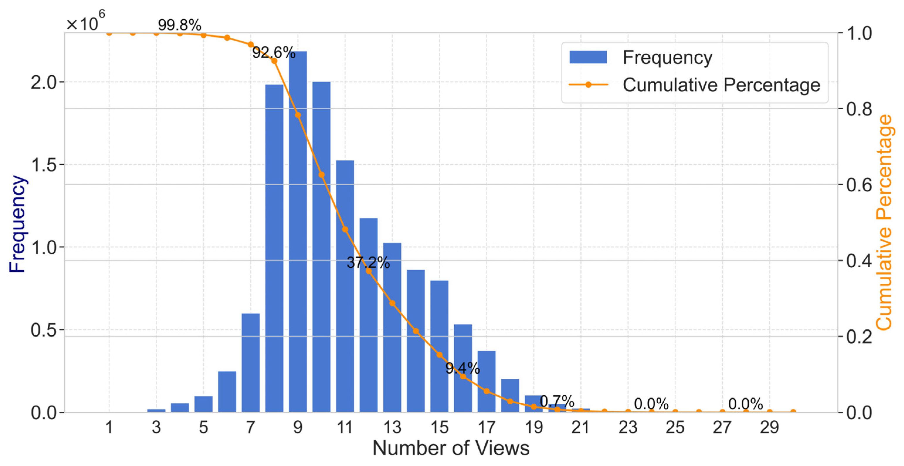
To ensure the representativeness of the modeling data and the accuracy of the model, a systematic analysis of the number of views distribution within WVCs was conducted, as shown in Figure 2. The horizontal axis denotes the number of views (i.e., how many times each WVC is observed), while the vertical axis represents the number of WVCs with view counts greater than or equal to the corresponding value. This cumulative distribution illustrates the coverage density of the observations. The yellow line indicates the proportion of data covered by WVCs with the corresponding number of views. Since each WVC is observed at least once, the curve starts from a view count of 1 and decreases monotonically, reflecting the diminishing number of WVCs that satisfy higher view thresholds. The statistical results demonstrate that WVCs with 1–3 views account for less than 2% of the total, while those with 4–7 views constitute the majority. Considering the trade-off between data sufficiency and model complexity, WVCs with four or more observations were selected for modeling, ensuring that the vast majority of valid data are retained. To ensure a consistent input structure for the model, only the first four observations of each WVC were used as input features. For WVCs with more than four views, the earliest four observations were selected based on the original data record order.

2.2. ERA5 Data

The ERA5 dataset from ECMWF (European Centre for Medium-Range Weather Forecasts) is employed as the reference for the true sea surface wind field in this study. As a fifth-generation reanalysis product, ERA5 delivers comprehensive high-resolution meteorological data across time and space since 1950, covering atmospheric, oceanic, and land systems globally. ERA5 is extensively applied in numerical weather prediction, climate research, and model evaluation and holds significant importance in ocean meteorological research as well [27]. The ERA5 wind field data serve as the target variable for the model. Throughout the training process, it is employed to compute the loss function and to guide the optimization of model parameters. Throughout the testing phase, it is utilized to assess the model’s generalization capability. Specifically, to correspond with satellite observation data, sea surface wind components (u, v) at an altitude of 10 m were selected over a section of the Pacific Ocean ranging from 40°N to 40°S latitude and 130°E to 120°W longitude. The data correspond to the first three days of each month in 2023 (36 days in total) and the first day of each month in 2024 (12 days in total), resulting in a total of 48 sampling days. It features a temporal resolution of one hour and a horizontal spatial resolution of 0.25 degrees.
The u and v components provided by ERA5 represent the zonal (east–west) and meridional (north–south) components of the wind, respectively. Based on these components, wind speed and wind direction can be derived. Wind speed is computed through vector synthesis of u and v , and wind direction is calculated using the following formula:
ϕ = m o d 180 + 180 π a t a n 2 u , v , 360
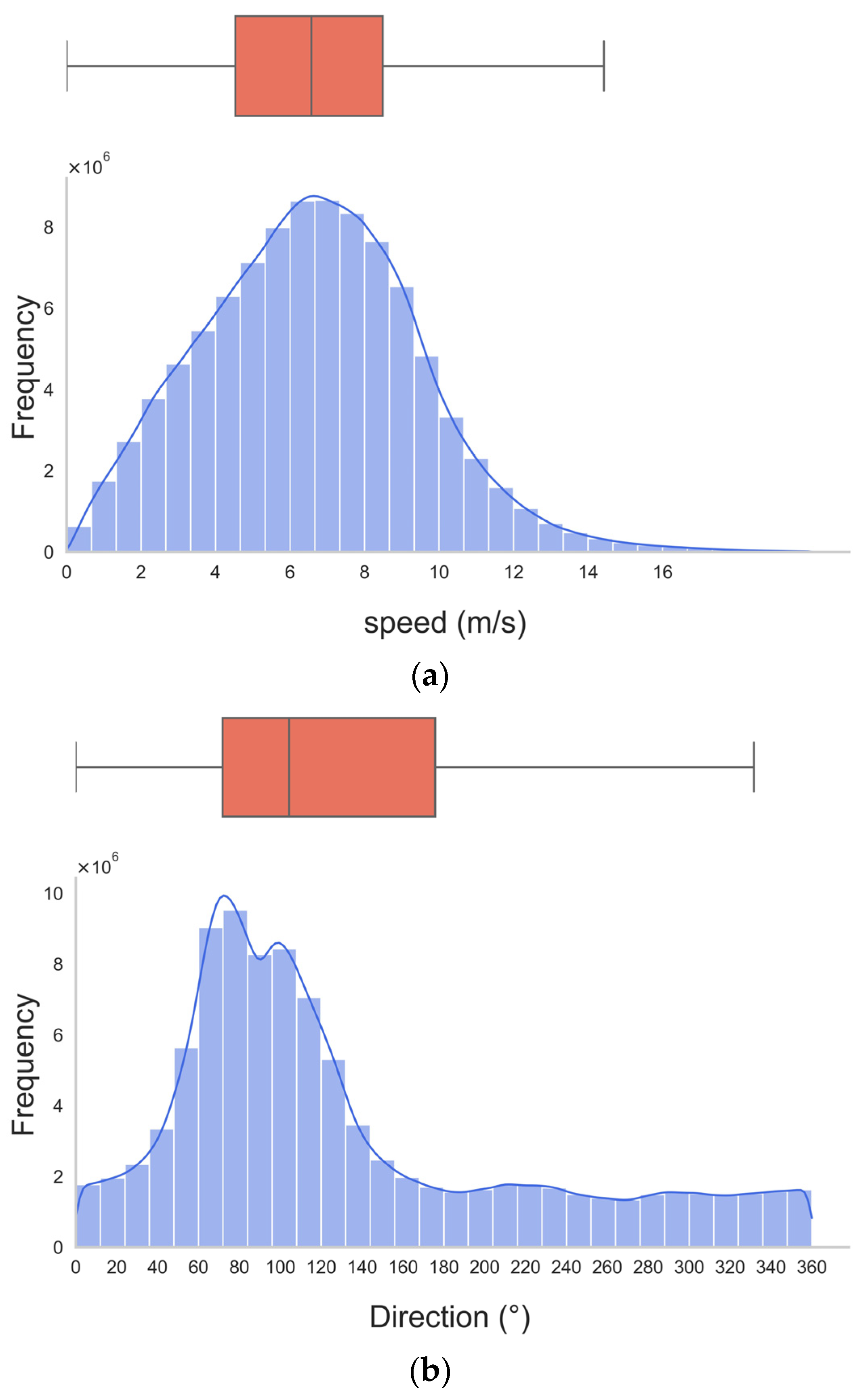
Figure 3 shows the overall statistical distributions of wind speed and wind direction in the selected dataset. The blue histograms represent the frequency distributions of wind speed and direction, while the dark red boxplots illustrate the interquartile range and median values. It is worth noting that the wind direction angles used in this study represent the direction from which the wind originates. For example, a wind direction of 90° indicates an easterly wind. As shown in the figure, wind speeds span a wide range, but the number of samples in high wind speed intervals is relatively low. The distribution of wind direction is uneven, with dominant directions primarily from the northeast and southeast.

2.3. TAO Data

The National Data Buoy Center (NDBC) provides extensive ocean observation data, including multiple TAO buoys deployed across the equatorial Pacific [28]. These buoys offer crucial in situ measurements for investigating ocean–atmosphere interactions in tropical regions. In this study, the temporal coverage of the TAO buoy data is consistent with that of satellite observations and ERA5 reanalysis products, focusing on a total of 48 representative dates across 2023 and 2024, specifically the first three days of every month in 2023 and the first day of every month in 2024. Spatially, 31 buoy stations were selected within the region spanning 165°E to 125°W and 8°N to 8°S, providing in situ wind observations over the equatorial Pacific. The TAO buoy data obtained from the official website include the u and v components of wind, representing wind conditions at a height of 4 m [29]. To ensure consistency with the ERA5 reanalysis data, these wind components at 4 m must be adjusted to correspond to the standard 10 m wind level. The conversion follows the formula below [30]:
V z = V r e f ln z z 0 ln z r e f z 0
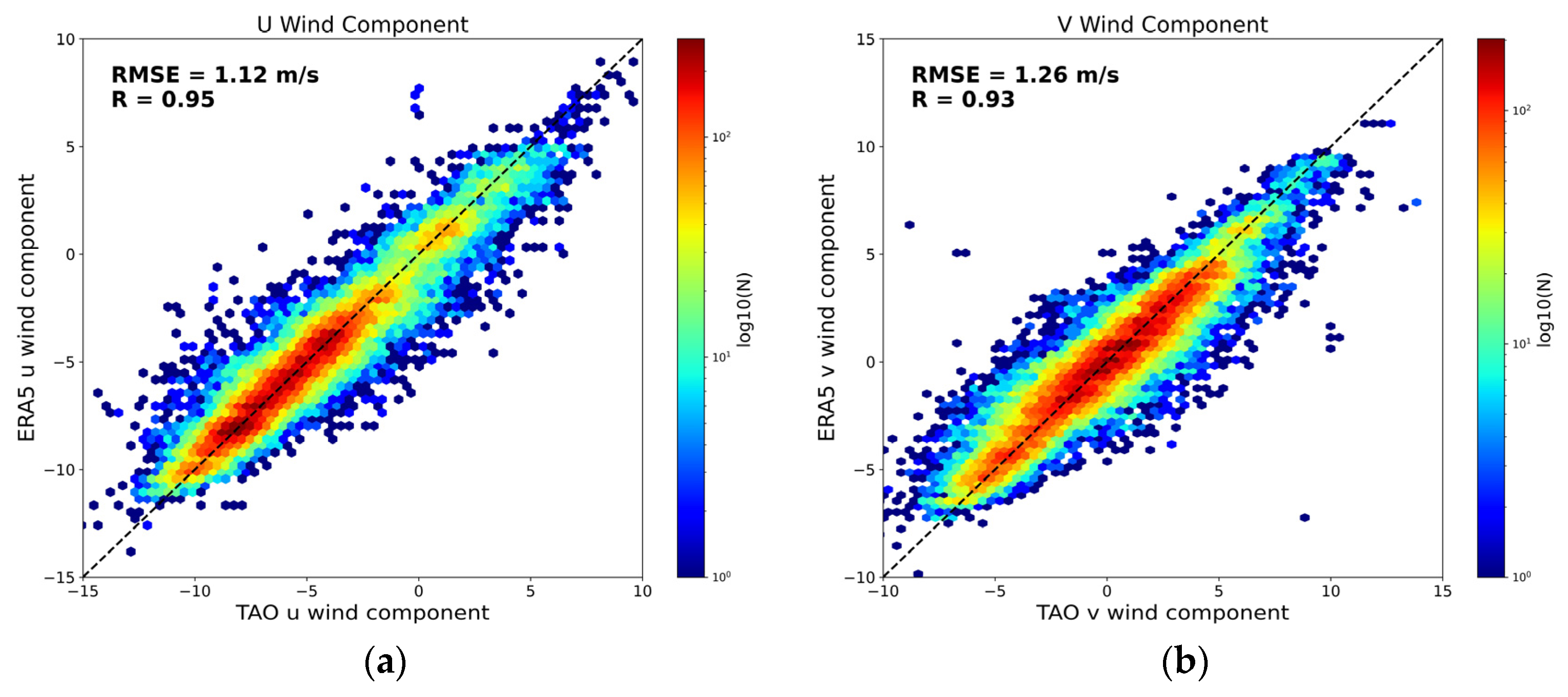
where z r e f is the reference height (i.e., the buoy’s wind measurement height), z is the extrapolated height (i.e., the wind measurement height of the ERA5 data), V r e f is the wind speed at the reference height, and V z is the wind speed at the extrapolated height. The parameter z 0 represents the sea surface roughness, which is taken as 0.0016 m in this study. Compared to reanalysis datasets, buoy-derived wind speed and direction are generally more representative of actual wind conditions due to their observational nature. However, the spatial coverage of buoy data is inherently limited by the sparse distribution of stations, making it insufficient to characterize broad, continuous wind fields. Therefore, in this study, TAO buoy observations are employed as an important reference to evaluate the accuracy of ERA5 reanalysis wind products. By analyzing the differences between ERA5 reanalysis data and in-situ buoy observations at the same time and location, the suitability and accuracy of ERA5 data for this study are assessed. Figure 4 presents scatterplots comparing the u and v wind components from ERA5 data and TAO buoy observations. The x-axis represents the TAO buoy wind component, while the y-axis shows the corresponding ERA5 value. The color of each scatter point reflects data density, with darker red indicating higher concentrations. A logarithmic color scale is used for the color bar, highlighting regions from sparse (lighter color) to dense (darker color) data distribution. Additionally, a diagonal reference line is included to indicate the ideal case where ERA5 and TAO wind components are in perfect agreement. The calculated RMSE for the u-component is 1.12 m/s, with a correlation coefficient (R) of 0.95. For the v-component, the RMSE is 1.26 m/s and R is 0.93. These high correlation values indicate that ERA5 data meet the accuracy requirements of this study and can be regarded as a reliable reference for true wind conditions.

2.4. BP Neural Network

Neural network methods have emerged in recent years as a prominent class of intelligent algorithms and are widely applied to solving various nonlinear problems [31,32], including disciplines related to environmental science and atmospheric remote sensing [33,34]. The BP neural network is a type of feedforward neural network that trains the model’s weights using the backpropagation algorithm [35]. The BP algorithm is a gradient descent-based learning method that updates the weights of each layer by computing the gradient of the error and propagating it backward. BP neural networks typically consist of multiple neurons and layers, and they employ nonlinear activation functions to establish complex correspondences between input variables and output results. A core advantage of the BP neural network is its ability to efficiently train deep networks, allowing it to address nonlinear problems that traditional machine learning algorithms struggle to handle.
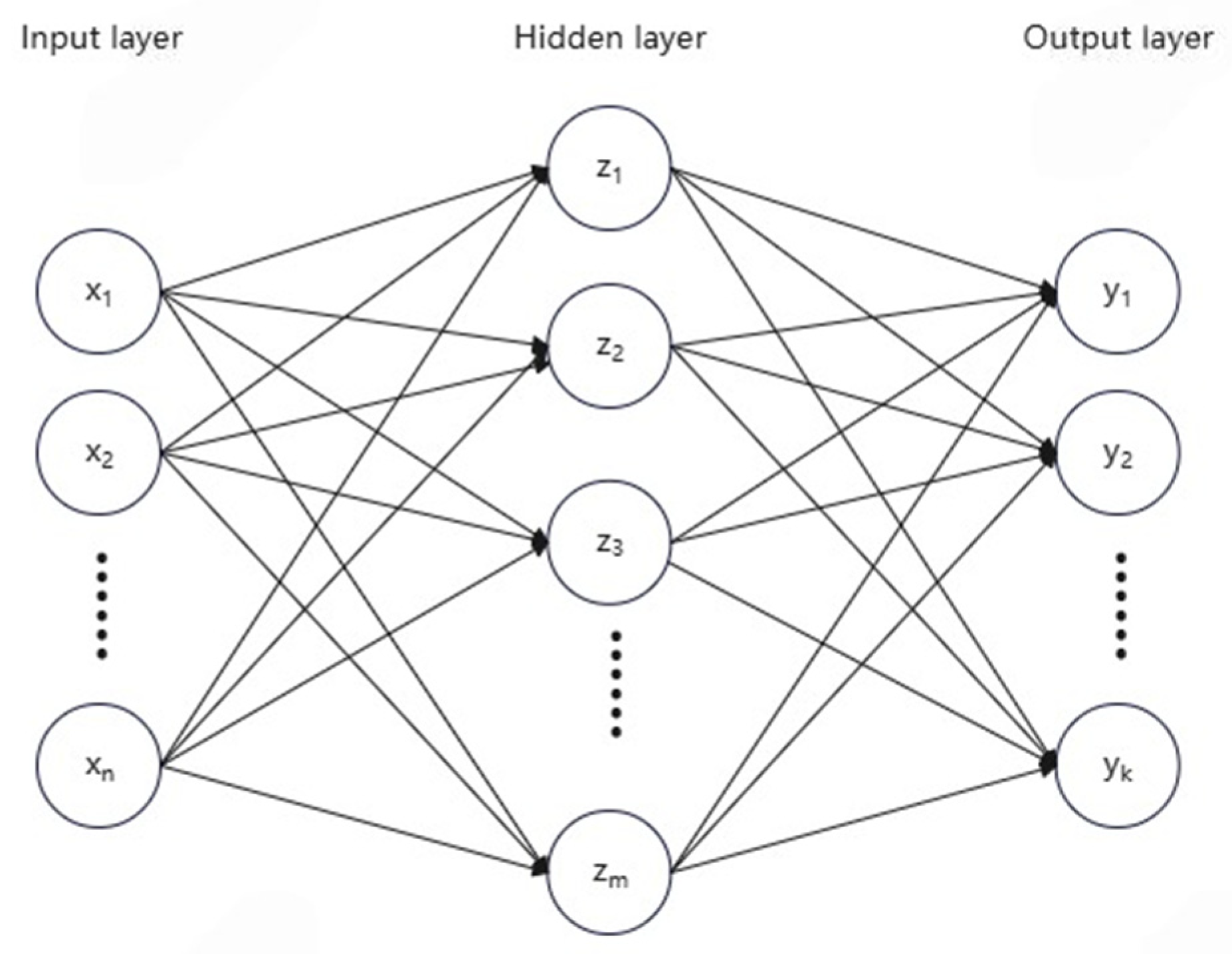
As shown in Figure 5, a typical BP neural network consists of an input layer, one or more hidden layers, and an output layer. The input layer accepts the original data and forwards it to the subsequent layer, with each neuron representing a single input feature. Each hidden layer contains multiple neurons, which are connected to neurons in the previous layer through weighted links and are responsible for extracting features and performing nonlinear transformations. The output layer delivers the ultimate output value or class label through its neurons.
The operation process of a BP neural network mainly consists of three steps: forward propagation, loss calculation, and backpropagation. First, the flow of data begins at the input layer until it reaches the output layer. This process is known as forward propagation. When signals pass from the input to the hidden layer, each hidden neuron performs a weighted sum of the input values plus a bias term, which can be expressed by the following formula:
z l = W l a l 1 + b l
Here, W l is the weight matrix, a l 1 represents the activated output originating from the preceding layer, b l is the bias term, and z l is the weighted input. To introduce nonlinearity, the network applies an activation function g(x) to the weighted input z l , resulting in the output of the current layer as follows:
a l = g z l
The activation functions used in this paper are Leaky ReLU [36] and Sigmoid [37]. Leaky ReLU is mathematically expressed as follows:
f x = x , if   x 0 α x , if   x < 0
Here, α represents a small positive parameter regulating the extent of leakage when the inputs are negative. Compared to ReLU, Leaky ReLU addresses the ‘dying neuron’ problem: when x ≤ 0 during computation, the derivative remains a constant, allowing the weights to continue updating, which helps alleviate the issue of weight stagnation in the negative input range. Sigmoid is mathematically expressed as follows:
f x = 1 1 + e x
In the output layer, an appropriate function is selected based on the task [38]. For regression problems, a linear transformation is typically used as follows:
a L = z L
The optimization of model parameters is facilitated by the loss function, which assesses the discrepancy between the model’s predictions a L and the real observations y. In the context of regression analysis, the mean squared error (MSE) is commonly employed. This metric is determined by the following calculation:
L = 1 m i = 1 m y i a i L 2
Here, m represents the batch size, which is the number of samples processed in one forward or backward propagation pass.
δ L = L z L = a L y
Here, δ L denotes the error at the output layer. Next, the chain rule is employed to propagate the error backward to the hidden layers.
δ l = W l + 1 T δ l + 1 g z l
Here, g z l represents the activation function’s gradient, and ⊙ denotes the element-wise (Hadamard) product. Then, the gradients of the biases and weights are computed as follows:
L W l = 1 m δ l a l 1 T
L b l = 1 m i = 1 m δ i l
To optimize the model parameters and minimize the loss function, the Adam optimizer is utilized. It computes the exponential moving averages of both the gradients and the squared gradients, enabling adaptive learning rate adjustment and promoting fast convergence [39].
Hereafter, the Mixture Density Network (MDN) structure is introduced to better address the inherent uncertainty and ambiguity in wind direction prediction [40]. Unlike traditional models that produce a single deterministic output, MDNs generate a conditional probability distribution over possible outcomes by predicting the parameters (means, variances, and weights) of a mixture of Gaussian components. This probabilistic framework is particularly well-suited for wind direction inversion, where similar input conditions may correspond to multiple plausible wind directions (i.e., the existence of ambiguous or multimodal solutions).
To enhance the expressive capacity and training effectiveness of the model, this study introduces residual connections based on the traditional BP neural network architecture [41]. Residual connections allow the input signal to bypass one or more hidden layers and be added directly to the output, effectively mitigating the vanishing gradient problem in deep networks. This facilitates better gradient flow and faster model convergence. In addition, residual structures help prevent network degradation, thereby improving the model’s generalization ability and robustness.

3. Results

In the previous section, the basic structure and input features of the BP neural network were introduced. Considering that the ERA5 data represent wind speed and direction through the u and v components, this study focuses on modeling these two components. After obtaining the predicted u and v values from the inversion model, wind speed and direction are subsequently derived and further evaluated. During neural network modeling, the data are commonly partitioned into two subsets: one for training and another for testing. The training subset is employed to optimize the model parameters and improve its learning capacity based on known samples, while the testing subset—kept separate from the training phase—is utilized to assess how well the model generalizes to new, unseen data. In this study, data from the year 2023 were used as the training dataset, while data from the year 2024 were employed as the test dataset to evaluate the model’s generalization performance. Due to an extensive number of neurons set in the model, various regularization techniques, including weight decay, Dropout, batch normalization, and Huber loss, have been incorporated [42,43]. These regularization methods help prevent overfitting of the model and enhance its generalization capability. At the end of each epoch, the model evaluates the training loss and adjusts the learning rate using a scheduling strategy. When training becomes stable, the learning rate is gradually reduced to promote stable convergence [44]. After training is completed, to verify the accuracy and generalization ability of the wind speed and wind direction models, evaluations are conducted using the test set. All subsequent models are based on the PyTorch framework (version 2.5.1), which is widely used in the field of deep learning research [45]. PyTorch employs dynamic computational graphs and provides a flexible and intuitive interface for defining and manipulating tensors. These features allow for more transparent and adaptable model design and debugging and make it easier to implement complex neural network architectures. In addition, PyTorch offers powerful GPU acceleration support, which can significantly improve the training efficiency of large-scale neural networks. These strengths render PyTorch a suitable framework for developing, training, and refining the deep learning architectures applied throughout this research.

3.1. Inversion of Wind Speed Components

3.1.1. Training Set for Wind Speed Components Model

Comprising an input layer, three hidden layers, and an output layer, the wind speed model adopts a five-layer neural network architecture. To comprehensively utilize the multi-frequency and multi-polarization measurements provided by the scatterometer, this study employs both Ku-band and C-band observations under HH and VV polarization modes as model input features. For each frequency–polarization combination, three physical parameters are extracted: azimuth angle, incidence (zenith) angle, and normalized radar cross-section (NRCS, i.e., backscattering coefficient). To enhance the angular diversity and observational robustness, four viewing geometries are selected for each WVC, resulting in 12 features per frequency–polarization combination. Considering the four combinations (Ku-H, Ku-V, C-H, and C-V), the model input layer ultimately consists of 48 features. This configuration is designed to fully exploit the spatial and physical information encoded in multi-angle, multi-band backscatter measurements, thereby improving the retrieval accuracy and generalization ability of the wind vector inversion model. Each layer incorporates dropout regularization to mitigate overfitting, as well as batch normalization to accelerate convergence and improve model stability [46]. The output layer consists of two neurons, corresponding to the u and v components of the wind vector.
In the modeling process, it is essential to determine an appropriate network architecture. Based on commonly used neural network configurations and insights gained from previous studies, four sets of hyperparameter combinations were designed and individually trained, and the structure yielding the best training performance was selected as the final model configuration. The details of each parameter combination are presented in Table 2. The purpose of this hyperparameter design is to compare the impact of different numbers of neurons when using different activation functions.
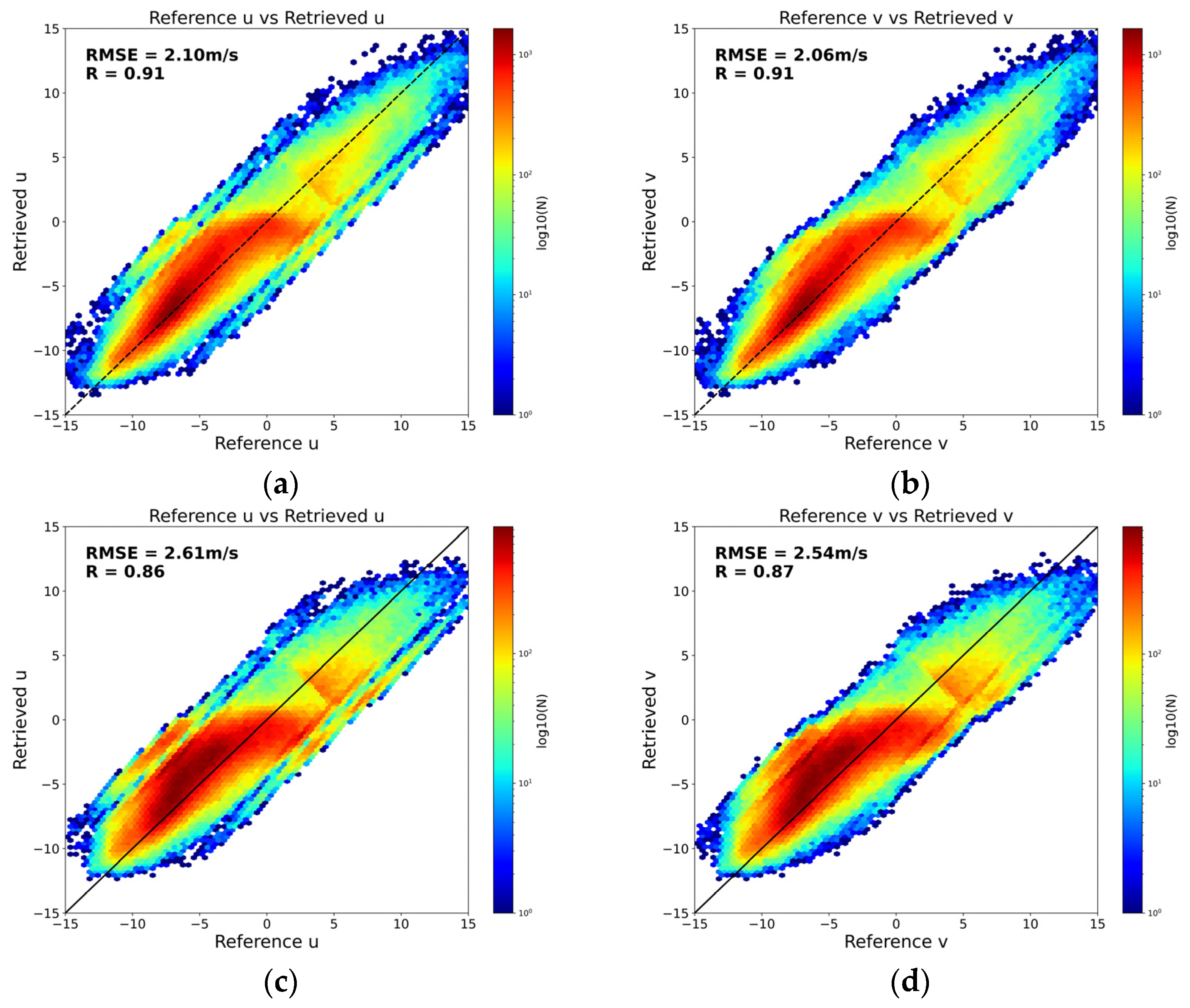
The following figures illustrate the performance of BP neural network models with different hyperparameter configurations in retrieving wind speed components. In each plot, the x-axis denotes the reference values, and the y-axis represents the retrieved values. A closer alignment to the diagonal line indicates better model accuracy. Figure 6 presents the training results for the first and second sets of hyperparameters. For the first group, the model achieved an RMSE of 2.10 m/s and an R of 0.91 for the u component and an RMSE of 2.06 m/s and an R of 0.91 for the v component, indicating good performance. In contrast, the second group (using the same network structure but with the sigmoid activation function) resulted in significantly higher errors: an RMSE of 2.61 m/s and R of 0.86 for u, and an RMSE of 2.54 m/s and R of 0.87 for v. These results demonstrate that, under the condition of fewer neurons, using Leaky ReLU significantly outperforms sigmoid.
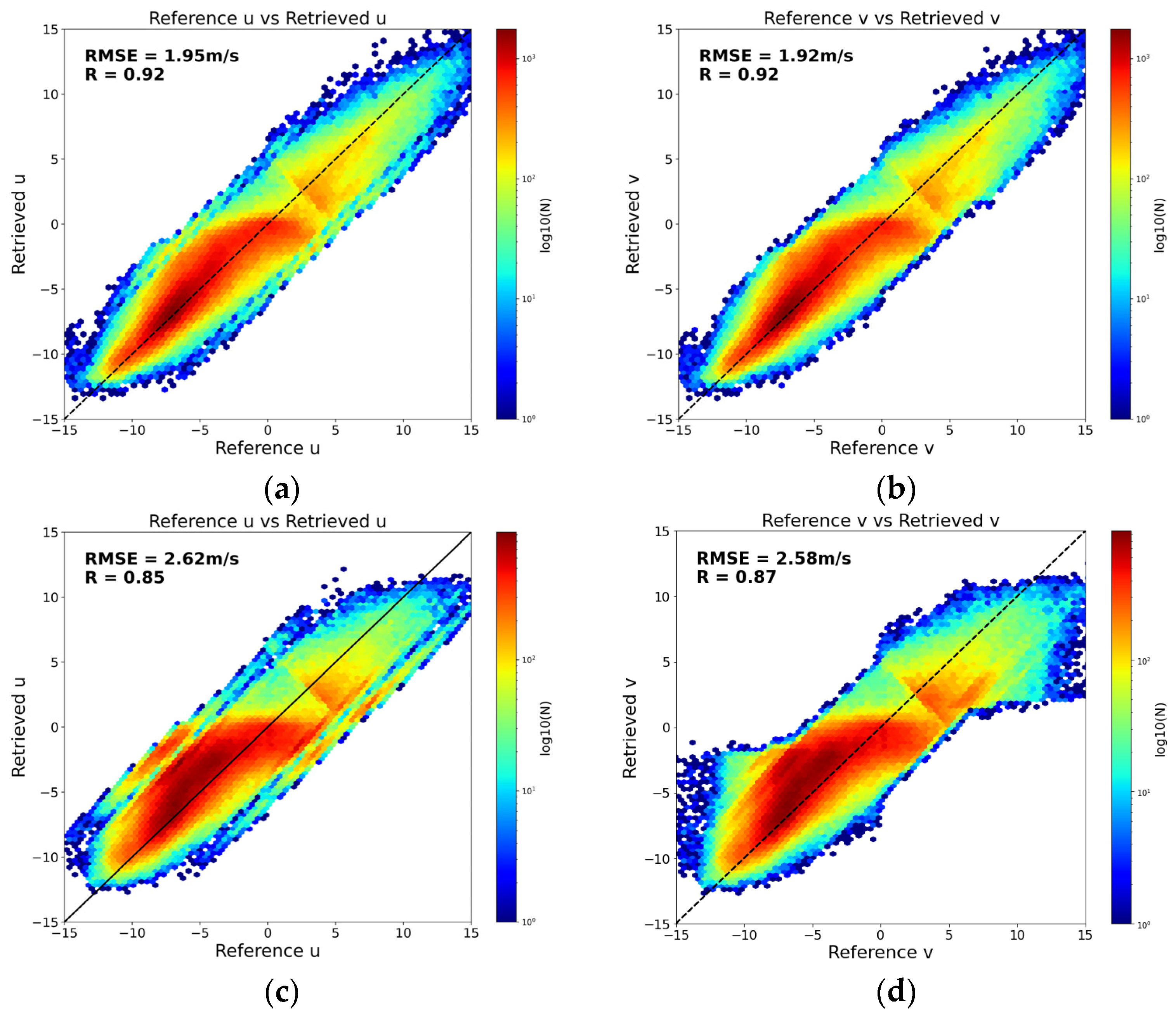
Figure 7 shows the training results for the third and fourth sets of hyperparameters. With a larger number of neurons, the third group (Leaky ReLU) again yielded strong performance: an RMSE of 1.95 m/s and R of 0.92 for u, and an RMSE of 1.92 m/s and R of 0.92 for v. The fourth group (sigmoid) produced RMSEs of 2.62 m/s for u and 2.58 m/s for v, with corresponding R values of 0.85 and 0.87. This further confirms that Leaky ReLU consistently outperforms sigmoid regardless of the neuron count. Moreover, a comparison across all four groups reveals that increasing the number of neurons—while keeping other settings unchanged—can lead to slight improvements in model performance. Table 3 summarizes the performance of the four hyperparameter combinations discussed above.
Overall, the scatter points are distributed closely along the diagonal in all models, indicating a clear linear relationship and demonstrating that each model is capable of accurately retrieving the u and v components of the wind field. In summary, the third hyperparameter combination can be considered optimal. It uses Leaky ReLU as the activation function and adopts a larger number of neurons in each hidden layer (1024, 512, and 256 neurons, respectively), resulting in the most accurate inversion performance.

3.1.2. Test Set for Wind Speed Components Model

For the test dataset, we fed the data into the previously trained inversion model. In accordance with the model’s input requirements, 48 observational variables—identical to those used during training—were provided. The model yielded the inverted u and v wind components for the test set. The results show that the inverted u component has an RMSE of 1.86 m/s and an R of 0.90 when compared to the reference values. For the v component, the RMSE is 1.85 m/s with an R value of 0.90. Although the performance is slightly lower than that on the training set, the overall inversion accuracy remains high. Figure 8 presents the scatter plots of the test results versus the reference values.

3.2. Validation of Wind Speed

3.2.1. Training Set Validation of Wind Speed

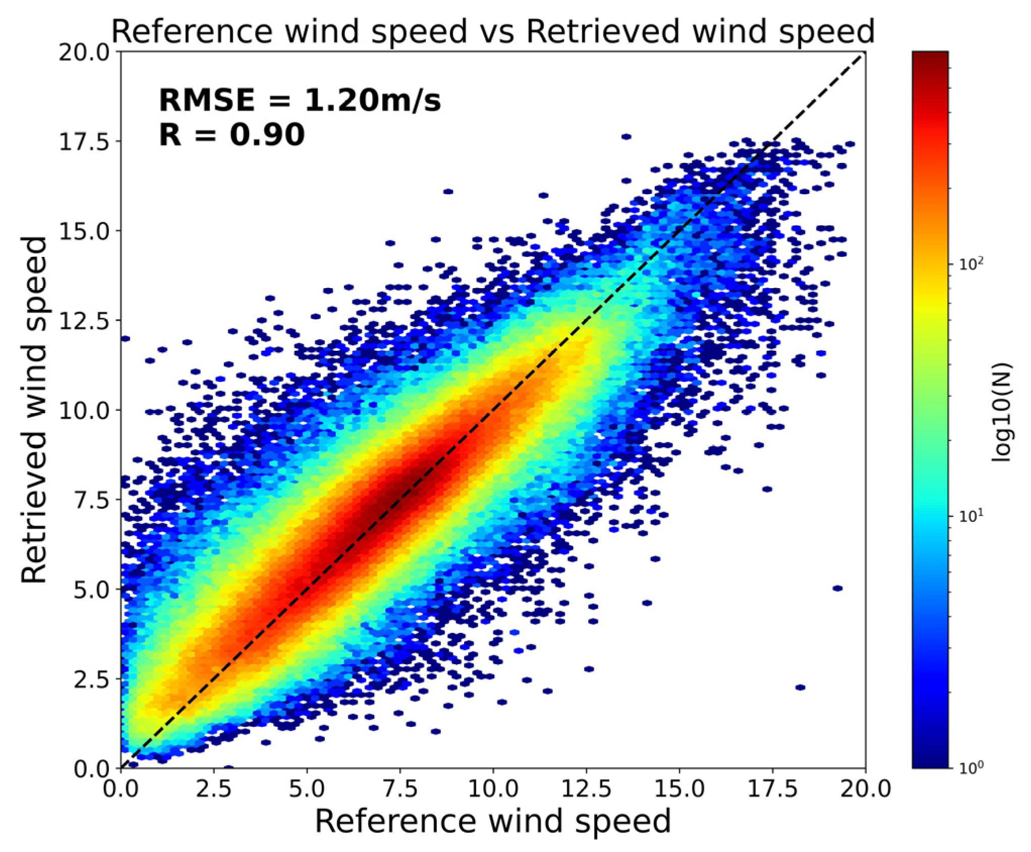
After obtaining the retrieved u and v components, wind speed can be derived through vector synthesis. Figure 9 presents the scatter fitting between the retrieved and reference wind speeds. Overall, the scatter points are closely distributed along the diagonal, indicating a clear linear relationship and further demonstrating that the model based on u and v component inversion can achieve high-accuracy wind speed retrieval. In terms of quantitative evaluation, the RMSE of wind speed on the training set is 1.20 m/s, and the R reaches 0.90, indicating strong agreement between the retrieved and reference values. These results confirm the reliability of the BP neural network in estimating sea surface wind speed. The RMSE values of the u and v components are higher than that of the total wind speed, indicating that the model performs better in capturing the relationship between wind speed magnitude and the input features, while its ability to predict wind direction is comparatively weaker. Moreover, the model performs best within the medium wind speed range, where the scatter points are more concentrated and closely aligned with the diagonal line. However, in the low wind speed range (0–3 m/s), certain retrievals exhibit lower accuracy, with the retrieved values tending to underestimate the reference values. This is primarily due to the limited spatial resolution of WindRAD, which makes it difficult to resolve the weak backscattering signals generated by wind speeds below 3 m/s. Table 1 specifies that the minimum detectable wind speed for both the C-band and Ku-band channels is 3 m/s. This suggests that the model has reduced sensitivity under low wind speed conditions.
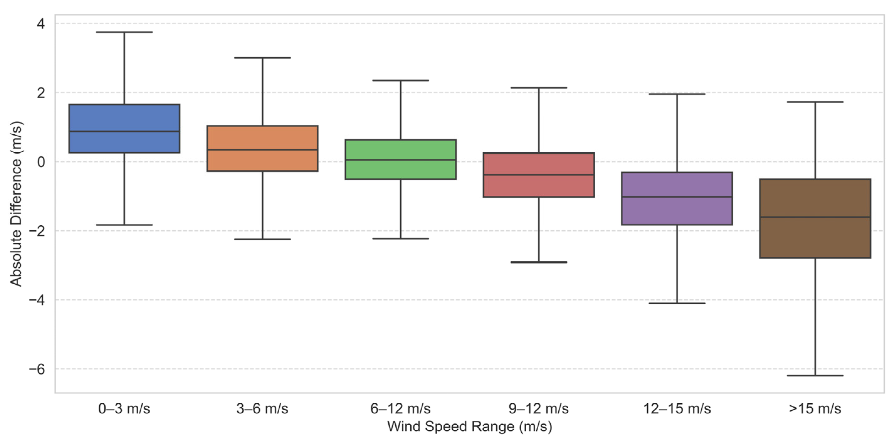
Figure 10 illustrates the distribution of absolute errors between retrieved and reference wind speeds across different wind speed intervals. The boxplot displays the median (central line), interquartile range (box), and the full data range (whiskers, excluding outliers). Together with Table 4, it provides a more detailed assessment of the model’s performance in each wind speed category. The mean error (MEAN) represents the average difference between the predicted and true values, while the standard deviation (STD) reflects the dispersion or stability of the prediction errors, indicating the model’s consistency. The model tends to overestimate wind speeds in low wind speed ranges and underestimate them in high wind speed ranges. This pattern is especially evident in the high wind speed interval (>15 m/s), where the underestimation becomes more pronounced, with a mean bias reaching −1.84 m/s. Such discrepancies may stem from an implicit conservative bias introduced by the loss function during training. Regarding error variability, the lowest standard deviation occurs in the 6–9 m/s range (0.06 m/s), suggesting greater model stability within this moderate wind speed interval. Notably, the model achieves optimal performance within the 6–12 m/s range, striking a favorable balance between accuracy (mean error: 0.06 to −0.42 m/s) and precision (standard deviation: 0.99–1.09 m/s). However, for wind speeds exceeding 15 m/s, the model’s performance deteriorates significantly, likely due to retrieval algorithm saturation or a lack of sufficient training samples under extreme conditions.

3.2.2. Test Set Validation of Wind Speed

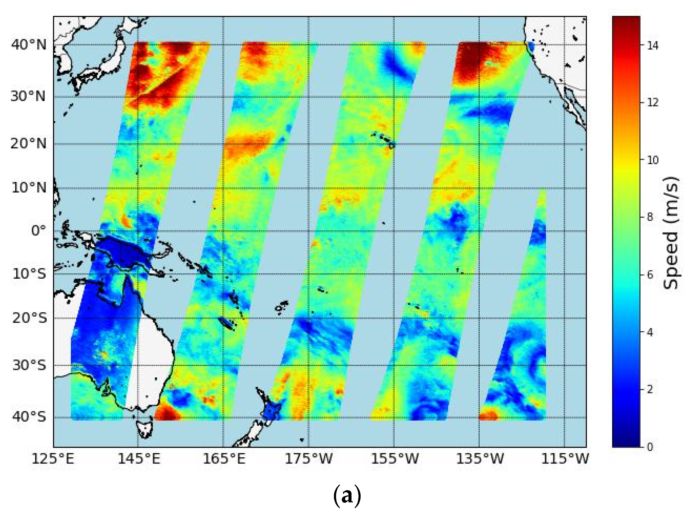
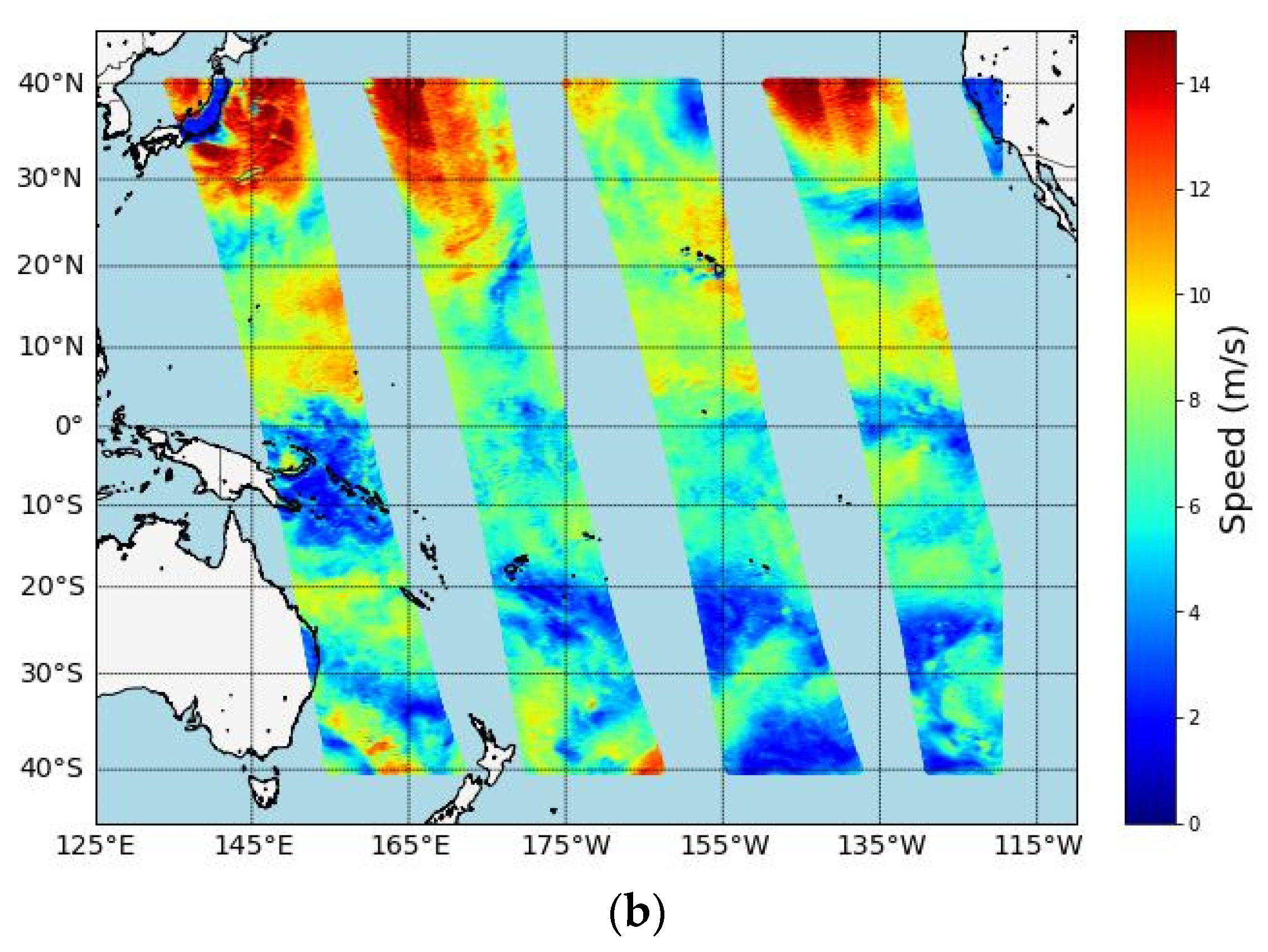
To further evaluate the accuracy of the wind speed retrieval, an in-depth analysis of the test dataset was conducted. As an example, the data from 1 March 2024 were visualized. Figure 11 presents the spatial distribution of the retrieved wind speed over the study area. In the figure, white indicates land, light blue represents ocean, and the other colors correspond to wind speed magnitudes. Higher wind speeds are shown in warmer tones such as red, while lower wind speeds are depicted in cooler shades like blue.
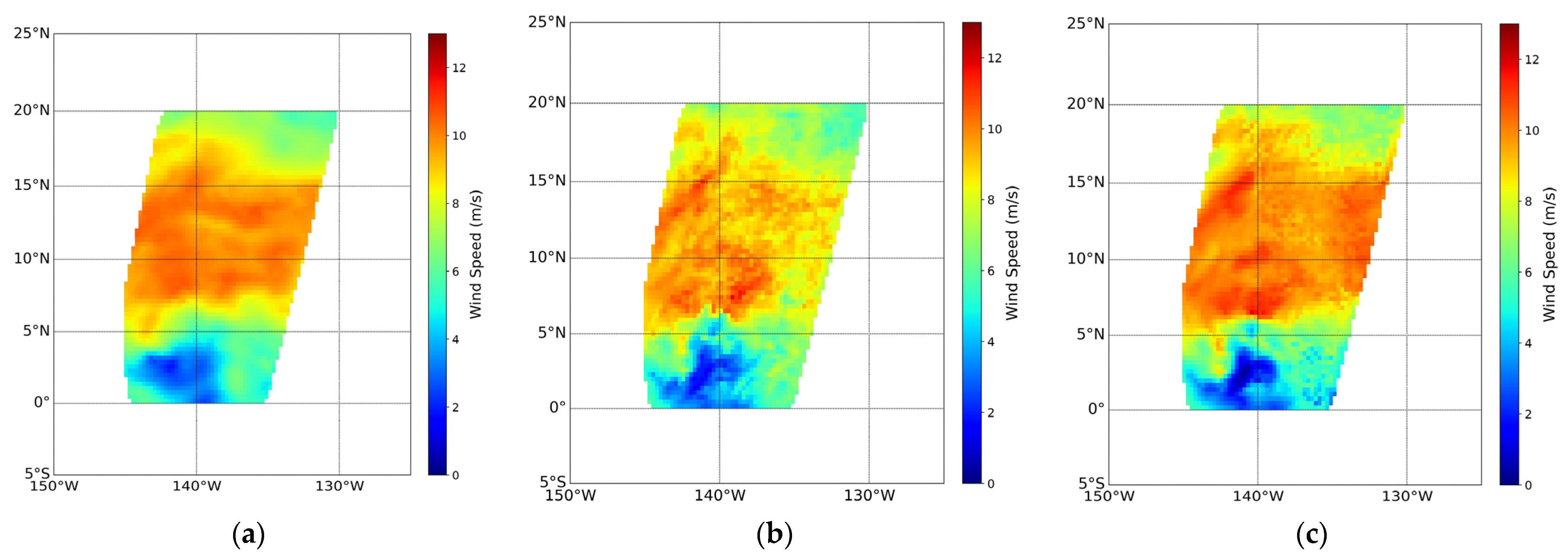
To comprehensively evaluate the performance of the BP neural network in estimating wind speed, this study compared the model’s retrieval results with the sea surface wind vector orbital product provided by FY-3E WindRAD. The analysis focused on data from 1 March 2024, using temporally and spatially matched samples among three datasets: ERA5 reference wind speed, wind speed retrieved by the BP model, and wind speed from the FY-3E orbital wind vector product. Based on this matched subset, the spatial distributions of wind speed derived from each data source were plotted and compared. Due to the filtering of unmatched samples during the spatiotemporal matching process, the test set results do not represent a complete coverage of the ocean surface. As shown in Figure 12, the wind speed estimated by the BP neural network aligns well with the reference wind speed across the study area. In contrast, the wind speed derived from the FY-3E satellite product exhibits evident overestimations in certain oceanic regions. Notably, the BP neural network demonstrates a strong ability to capture fine-scale wind field structures, which can be attributed to its powerful nonlinear fitting capability.
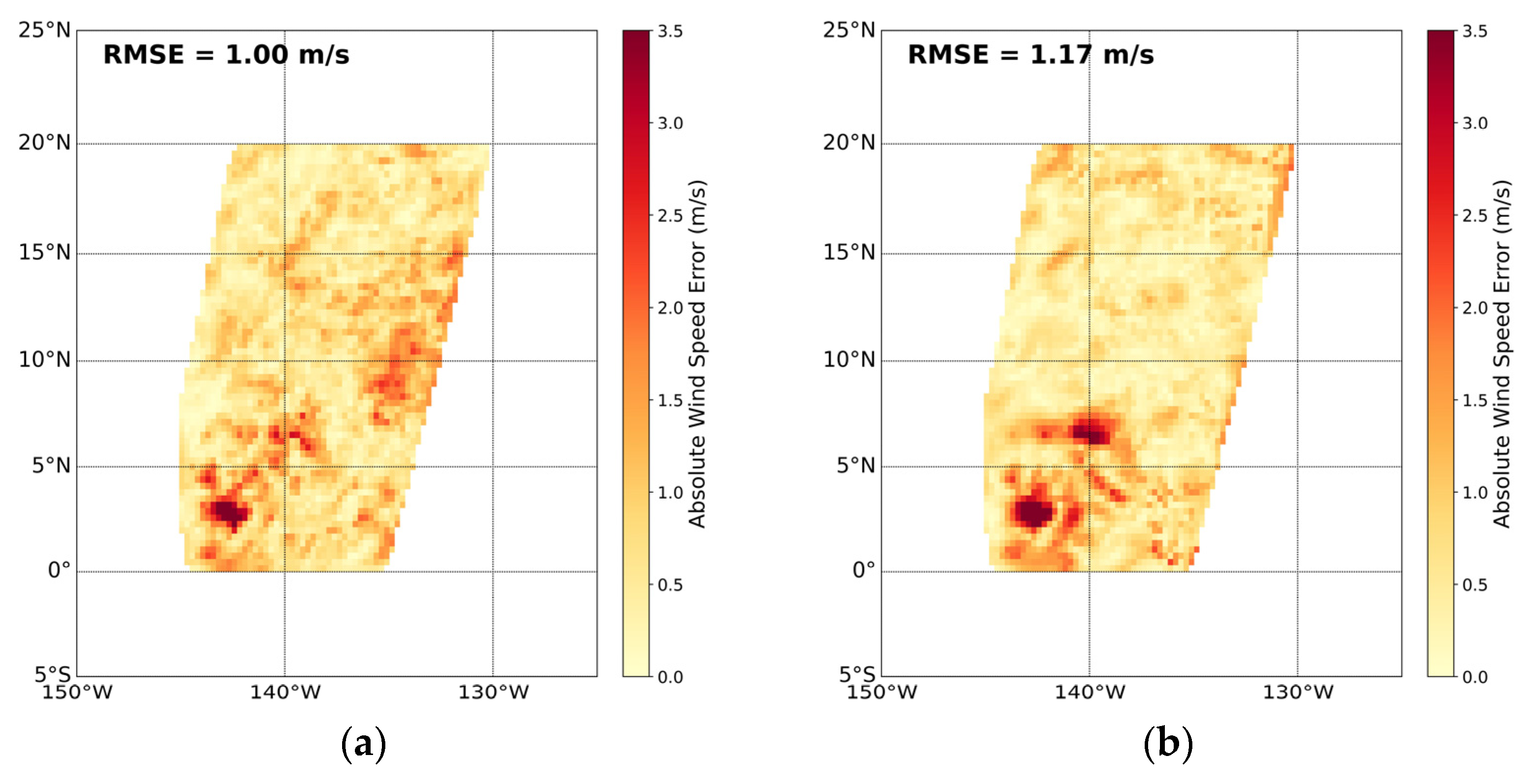
To provide a clearer depiction of the model’s inversion errors and the satellite product’s bias, RMSE distribution maps were generated for both the BP neural network-retrieved wind speed and the WindRAD Level-2 product wind speed, using ERA5 as the reference, as shown in Figure 13. In these maps, RMSE magnitude is visualized through color intensity: lighter shades indicate smaller errors, while darker tones represent larger discrepancies. Overall, the RMSE maps are predominantly light-colored, suggesting that low error levels are observed across most regions, with only a few localized areas showing elevated discrepancies. Quantitatively, the BP neural network achieved an RMSE of 1.00 m/s, whereas the WindRAD product resulted in an RMSE of 1.17 m/s. These results indicate that, within the selected temporal and spatial domain, the retrieval accuracy of the BP neural network significantly surpasses that of the satellite product. In the region between 0–5°N and 145–140°W, both the BP neural network retrievals and the satellite Level-2 wind vector products show significant discrepancies compared to the reference wind speeds. However, compared with the satellite-derived results, the BP model predictions exhibit better agreement with the reference data, demonstrating the model’s strong adaptability and robustness under complex wind field conditions. The observed errors in this region may be attributed to localized and complex atmospheric dynamics, such as frequent convective activity, intense vertical motions, and abrupt changes in wind field structure—all of which significantly increase the difficulty of wind speed retrieval.

3.3. Validation of Wind Direction

3.3.1. Training Set Validation of Wind Direction

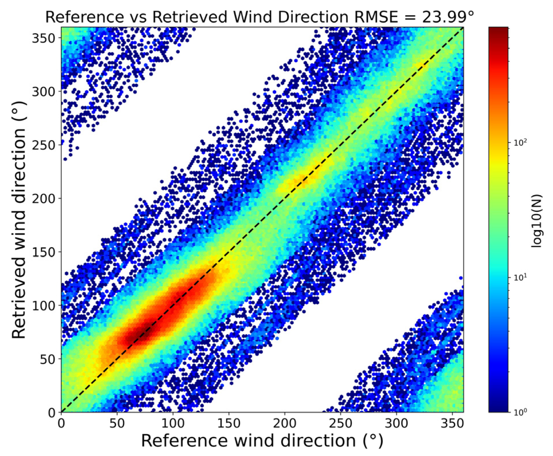
As described in Equation (1), wind direction can be calculated from the retrieved u and v components. After deriving wind direction from the inversion results, the model’s performance in capturing wind direction was further evaluated. Figure 14 presents a scatter plot based on the training dataset, where the horizontal axis represents the observed wind direction and the vertical axis corresponds to the wind direction predicted by the BP neural network. The distribution pattern of the scatter points visually illustrates the model’s capability in approximating reference wind direction. The scatter plot shows that most data points are concentrated near the 1:1 diagonal line, indicating that the model exhibits good performance in wind direction retrieval. Some large directional errors appear near 0° and 360°, which can be attributed to the circular nature of wind direction—where 0° and 360° represent the same direction. The overall RMSE of wind direction on the training set is calculated to be 23.99°, suggesting a high level of retrieval accuracy.
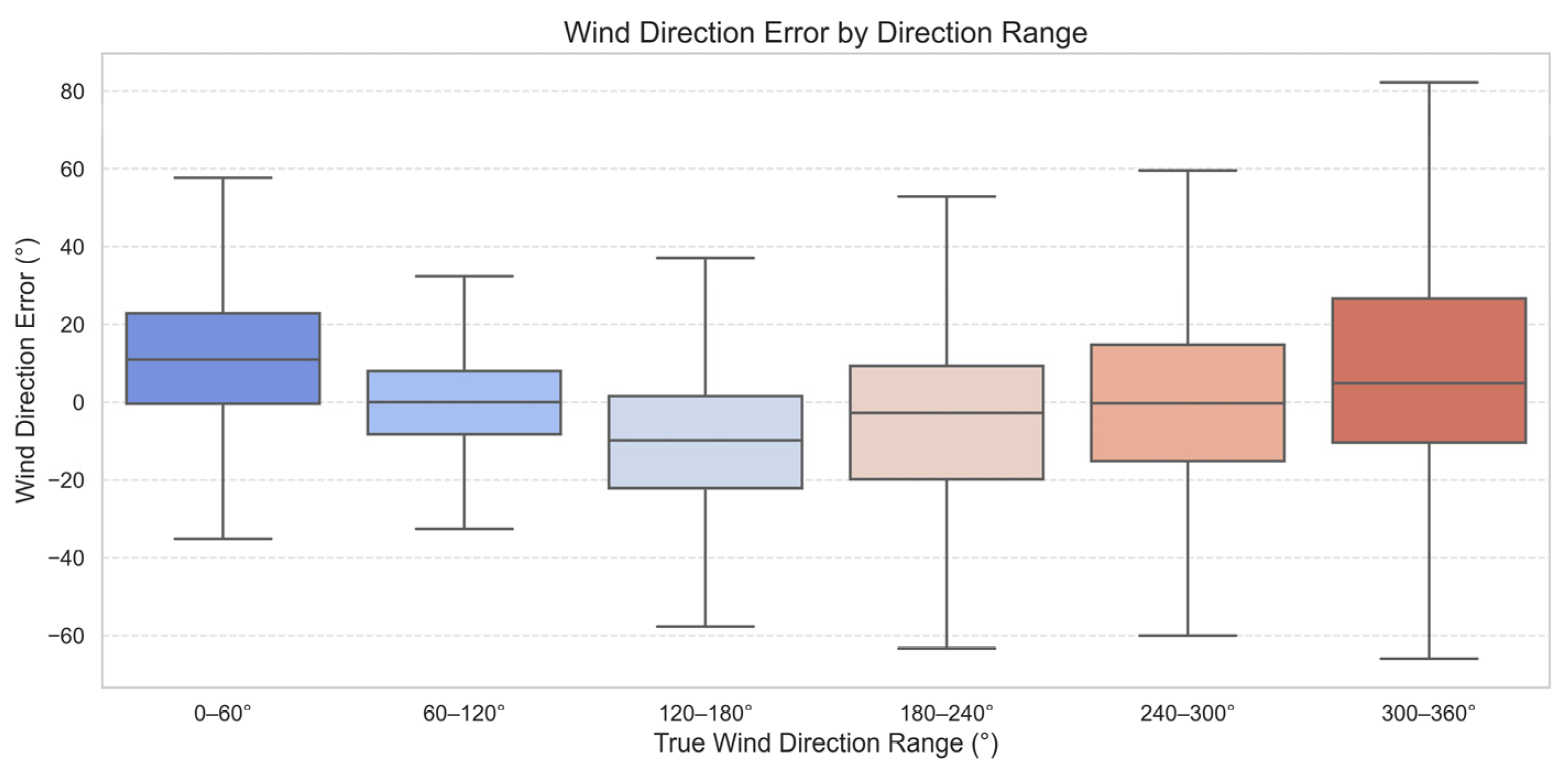
Figure 15 presents the distribution of wind direction retrieval errors across different true wind direction sectors using boxplots. In conjunction with Table 5, the results reveal consistent patterns in model performance across various wind direction intervals. In terms of bias, a pronounced underestimation is observed in the 120–180° sector, with a mean error of –10.57°. Although the 240–300° sector shows a relatively small average bias (+1.44°), it exhibits a high standard deviation of 31.95°, indicating considerable local variability and possible instability in retrieval performance—potentially due to abrupt wind direction changes or geometric limitations of satellite viewing angles. In contrast, the 60–120° sector demonstrates the most accurate and stable retrieval results, with near-zero mean bias and relatively low variability. Notably, the 60–120° sector has the lowest standard deviation (16.04°), suggesting high consistency in the model’s predictions of easterly winds. This superior performance can likely be attributed to the data characteristics: within the selected temporal and spatial domain, easterly winds prevail over the Pacific Ocean, resulting in a higher representation of such wind directions in the training set and enhancing the model’s learning efficiency in this sector. Overall, although the model exhibits systematic bias in certain wind direction sectors (e.g., 180–240°), the mean error across the entire wind direction spectrum remains within a relatively small range. In particular, the 60–120° sector demonstrates outstanding performance in both accuracy (mean bias) and stability (standard deviation), confirming the model’s strong generalization capability and robustness in representing prevailing wind directions.

3.3.2. Test Set Validation of Wind Direction

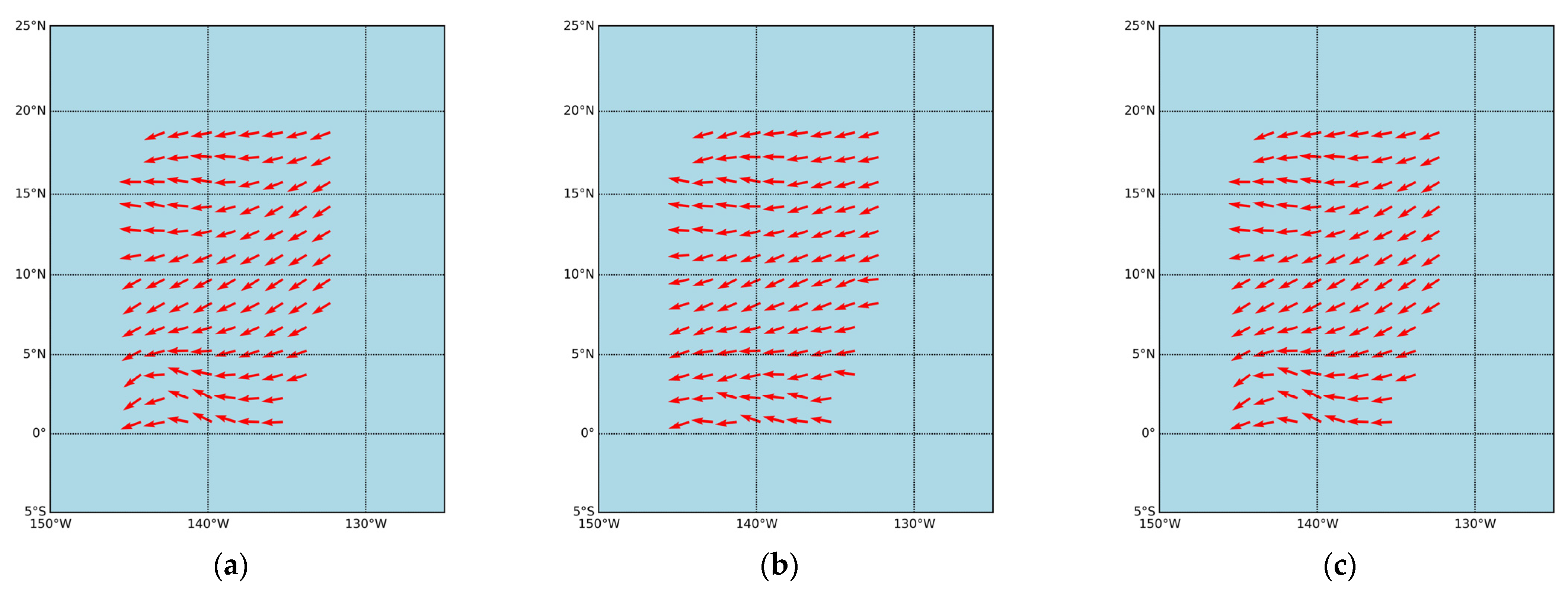
To evaluate the wind direction retrieval performance of the model on the test dataset, this study selected spatially and temporally matched samples from three sources: ERA5 reference wind data, BP model-estimated wind data, and the FY-3E orbital wind vector product. To ensure clarity and comparability in visualization, all wind direction data were averaged over 1.5° × 1.5° latitude–longitude grids. A partial wind field on 1 March 2024, was used as an example for wind vector visualization. Figure 16 presents the spatial distribution of wind directions over the study area for the three datasets. As shown in the figure, the wind direction field retrieved by the BP neural network exhibits good overall agreement with the reference ERA5 wind field, demonstrating the model’s strong capability in extracting wind direction features and effectively capturing the dominant structure of the sea surface wind field. Further analysis of the region near the equator (0–5°N) reveals a more complex wind direction pattern in the ERA5 wind field. Unlike other areas within the study region, which are predominantly influenced by northeasterly or southeasterly flows, this area exhibits a clear tendency toward convergence. This finding supports the hypothesis proposed in Section 3.2.2, which suggests a structurally complex wind field in this region.
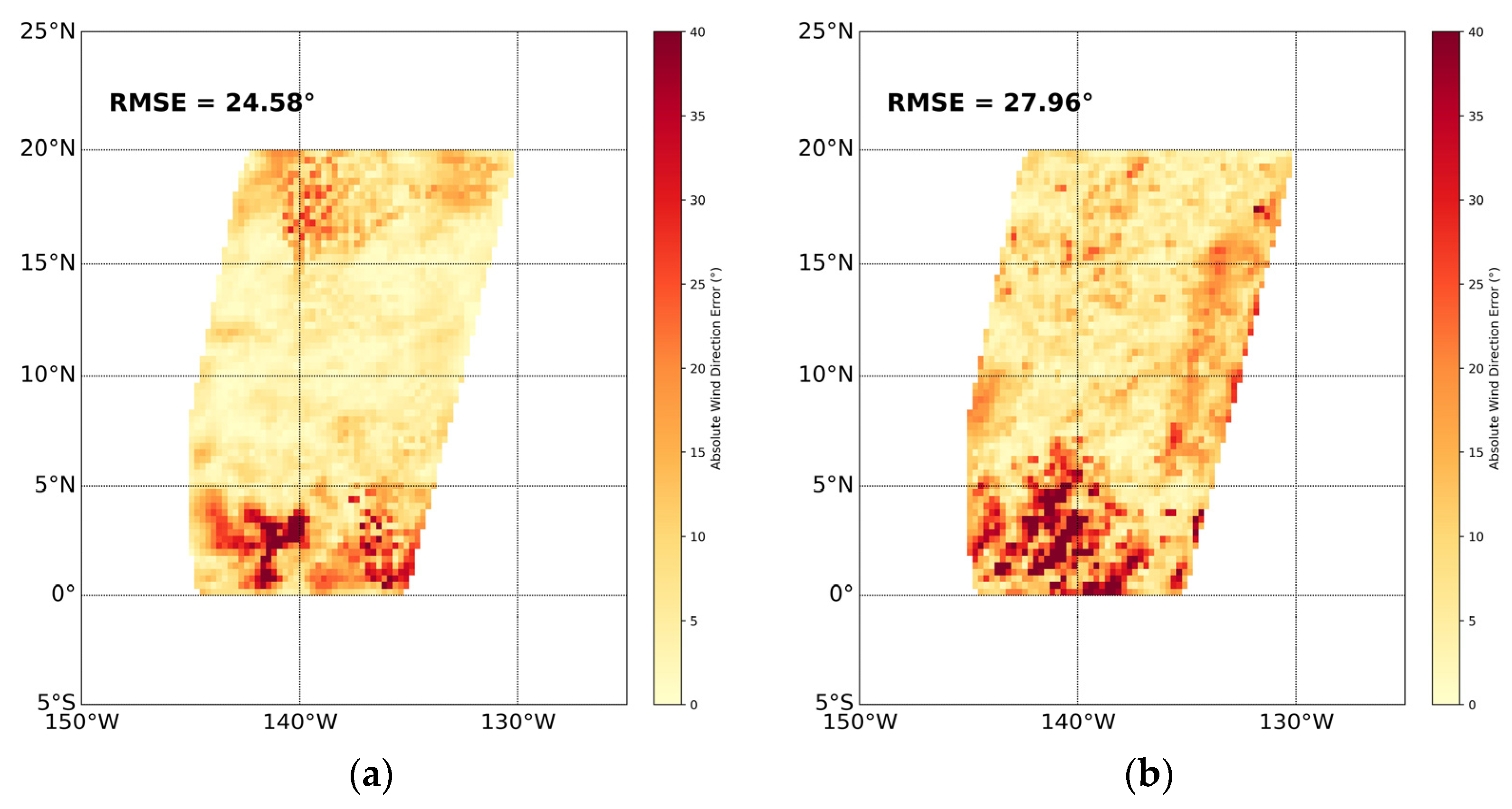
To further quantify the retrieval errors and compare the performance of different wind direction sources, this study calculated the RMSE distribution maps between the BP neural network-retrieved wind direction and the ERA5 reference wind direction, as well as between the WindRAD L1-level product and ERA5. They were presented in Figure 17. The RMSE heatmap for the BP neural network model exhibited predominantly lighter color tones, indicating relatively low error values across most regions, with no distinct high-error zones observed. In contrast, the RMSE heatmap for the WindRAD product revealed several localized areas with substantially higher deviations from the ERA5 reference. From a statistical perspective, the overall RMSE for the BP neural network-retrieved wind direction was 24.58°, whereas the RMSE for the WindRAD product reached 27.96°. These findings clearly demonstrate that the BP neural network offers significantly higher accuracy in wind direction retrieval compared to the current WindRAD L1-level satellite product.

3.4. Validation with TAO Buoy Data

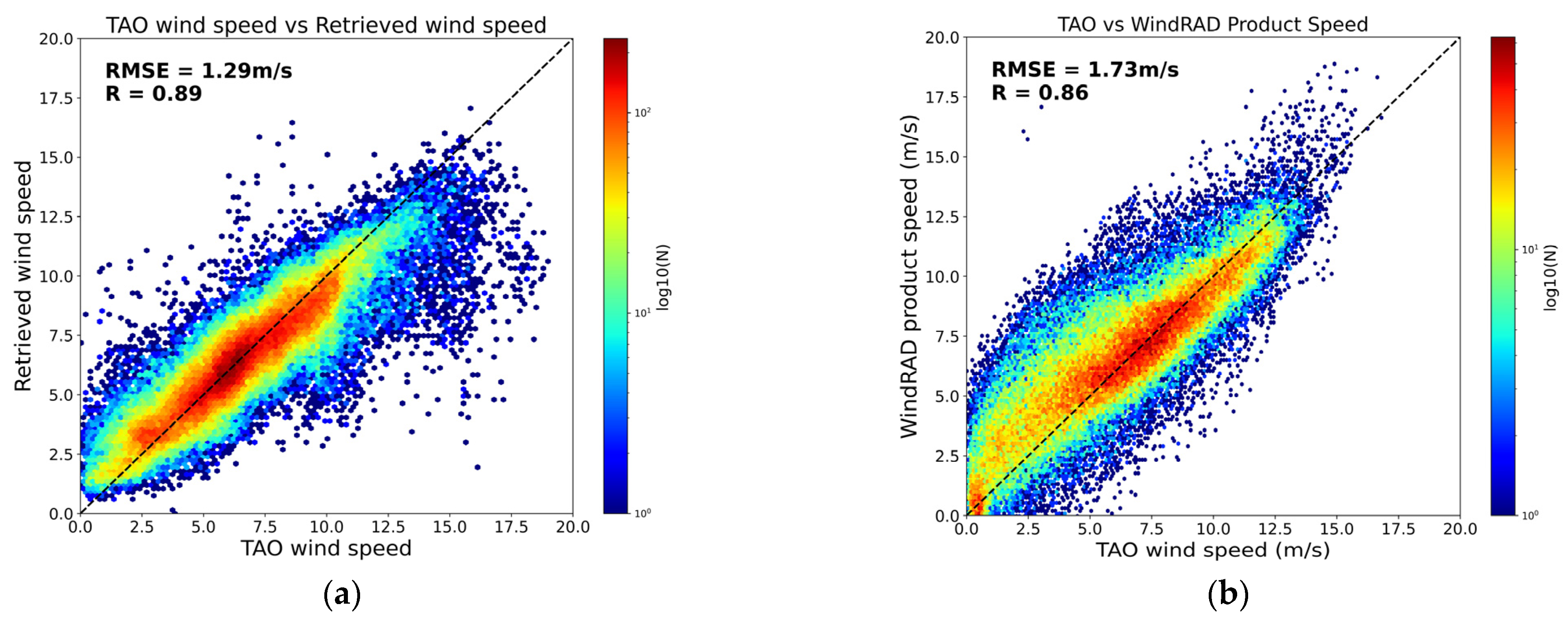
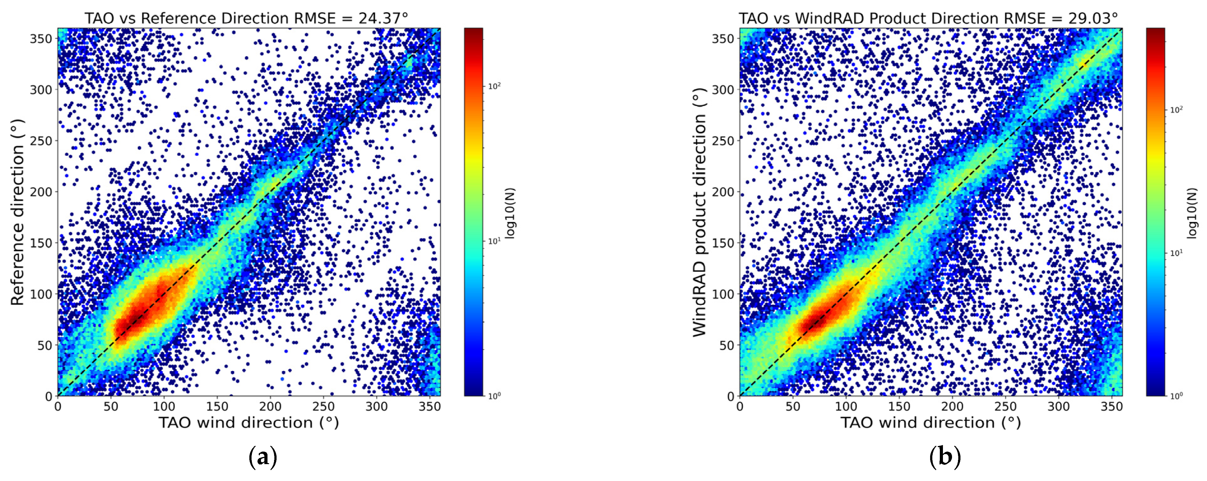
To further assess the applicability and accuracy of the retrieval model under real-world observational conditions, this study introduces in situ wind measurements from the TAO (Tropical Atmosphere Ocean) buoy network as an independent reference dataset. These observations are used to evaluate the model’s performance in estimating wind speed and direction. In addition, comparisons are made with the FY-3E WindRAD orbital wind vector product to highlight the advantages of the proposed method in terms of retrieval accuracy. Figure 18 presents scatter plots comparing the BP neural network-retrieved wind speeds with TAO buoy observations, along with the comparison between WindRAD product wind speeds and TAO data. The results show that the BP model demonstrates stronger linear correlation with TAO measurements, lower errors, and improved fitting accuracy with an RMSE of 1.29 m/s. Correspondingly, Figure 19 shows the scatter plots comparing wind direction retrieved by the BP model and the WindRAD product against TAO observations. The BP model again outperforms the satellite product, achieving a lower overall RMSE of 24.37°, along with higher correlation. In summary, the comparison with TAO buoy observations further confirms the effectiveness and superiority of the BP neural network model in estimating both wind speed and direction. The results demonstrate that the model offers greater stability and applicability, particularly in realistic oceanic conditions.

4. Discussion

A key goal of the present research involved building a reliable model to represent the complex nonlinear interaction between backscattered microwave signals from satellites and sea surface wind structures. By incorporating a BP neural network algorithm and utilizing multi-angular observational data, this study aimed to enhance the retrieval accuracy of FY-3E WindRAD measurements and effectively address the wind direction ambiguity frequently encountered in traditional GMF-based retrieval methods. An important innovation of this study lies in the use of multi-view geometric and backscattering characteristics across different frequency bands and polarizations as model inputs, which significantly improves model adaptability to heterogeneous atmospheric and oceanic conditions, thereby providing a more generalizable and robust framework for operational wind field retrieval.
Drawing upon the findings outlined earlier, the retrieval models for both wind velocity and direction constructed in the current study demonstrate notable accuracy. Using ERA5 wind data as the reference, the model achieved an RMSE of 1.20 m/s for wind speed and 23.99° for wind direction on the training dataset. On the selected portion of the test set, the model maintained similarly high accuracy, with an RMSE of 1.00 m/s for wind speed and 24.58° for wind direction. Given that the test data are independent of the training data, it can be concluded that both models generalize well and do not suffer from overfitting [47]. Under the PyTorch framework, the model benefits from GPU acceleration, enabling high-speed training and excellent computational efficiency. Moreover, since the input features are limited to backscattering coefficients, azimuth angles, and zenith angles under different polarization modes, the model exhibits strong generalizability and transferability—provided that the radar observation accuracy is ensured.
The wind speed retrieval model exhibits high accuracy in the moderate wind speed range, primarily due to the greater number of samples and more uniform data distribution within the 4–10 m/s interval. These factors contribute to more effective learning of underlying patterns during the training process. However, the training results of the wind speed model reveal notable deviations in both the low (0–2 m/s) and high (>12 m/s) wind speed ranges, indicating limited accuracy in these specific intervals. These deviations could stem from an insufficient representation of extreme wind speed cases—both low and high—in the training dataset, which hampers generalization performance of the model within these specific settings. Additionally, low wind speeds may be more susceptible to background noise, while high wind speeds often exhibit stronger nonlinear characteristics, making accurate fitting more challenging. In addition, due to the resolution limitations of the instrument itself, the wind speed retrieval performance in the 0–3 m/s range is relatively less accurate.
The model shows direction-dependent performance. Significant underestimation occurs in the 180–240° sector, while the 240–300° sector shows high variability despite a small average bias. In contrast, the 60–120° and 300–360° sectors exhibit the best performance, with near-zero bias and lower variability, especially in the 60–120° sector (STD: 16.04°). This can be attributed to the dominance of easterly winds in the training data. Overall, the model maintains acceptable accuracy across all sectors, with particularly strong generalization in prevailing wind directions.
From the above discussion, the wind speed dataset utilized in the present study proves to be relatively comprehensive, covering the majority of sea surface wind speed variations. The training dataset demonstrates strong representativeness. But influenced by large-scale circulation systems such as the Northeast and Southeast trade winds, the wind direction distribution in the Pacific—particularly near the equator—is notably uneven. Consequently, although the total amount of wind direction data is substantial, regional biases in distribution make it challenging to achieve balanced coverage across the full 0–360° directional spectrum, which may affect model performance in certain directional sectors.
Nevertheless, the BP neural network-based retrieval models developed in this study exhibit robust generalization ability and high retrieval accuracy, especially within moderate wind speed intervals (4–10 m/s) and dominant wind direction sectors. The models incorporate comprehensive input features by integrating multi-view and multi-polarization backscatter coefficients, azimuth angles, and incidence angles, thereby fully capturing the scattering characteristics.
Compared to traditional geophysical model functions (GMFs), BP neural networks possess inherent advantages in modeling complex nonlinear relationships, enabling them to better capture the intricate coupling mechanisms between backscatter signals and wind fields and effectively mitigate longstanding issues such as directional ambiguity. Furthermore, the proposed models offer efficient training, flexible architectures, and scalability, making them highly suitable for large-scale remote sensing data processing and analysis. This study’s models thus hold promising potential for fine-scale oceanic wind field retrieval and wind resource assessment in practical applications.
Overall, the model constructed using the backpropagation neural network not only achieves the precision required for standard operational wind products but also maintains strong consistency with actual wind field conditions and demonstrates closer agreement with the true wind field compared to the FY-3E wind vector orbital product, thereby fulfilling the original objective of this study. These results indicate that the proposed method is both accurate and generalizable, with strong adaptability to heterogeneous atmospheric and oceanic environments. By integrating multi-angle backscattering and geometric features, the BP neural network model can alleviate wind direction ambiguity and accurately capture the inherent nonlinear complexities of radar observations. Importantly, this approach offers tangible benefits for real-world applications: it can enhance the quality of satellite-derived wind data for assimilation into numerical weather prediction and climate models, support maritime safety through more reliable wind monitoring, and contribute to renewable energy planning by providing improved offshore wind assessments. As such, this study underscores the capability of neural network-powered retrieval methods to support the evolution of next-generation wind field products.

5. Final Remarks

The complex nonlinear relationship between the backscattered echo data received by radar and the sea surface wind field has long been a central focus in wind field retrieval research. Traditional Geophysical Model Function (GMF)-based methods often encounter the problem of wind direction ambiguity when modeling this relationship. In this study, a Backpropagation (BP) neural network model was developed to retrieve ocean surface wind field information using Level-1 data from the FY-3E satellite’s WindRAD instrument. In order to assess model accuracy, the data were partitioned into training and test subsets. The principal results of the present study can be outlined as follows:
(1)
In this research, observational geometry from four distinct satellite viewing directions was incorporated as input features into a Backpropagation (BP) neural network to estimate ocean surface wind fields. The findings indicate that the BP network effectively learns and represents the intricate nonlinear dependencies between remote sensing observations and wind field characteristics. Compared with conventional retrieval techniques that rely on geophysical model functions (GMFs), the neural network approach demonstrates enhanced adaptability and robustness, especially under complex and variable atmospheric conditions.
(2)
Model evaluation metrics demonstrated robust performance, with training set errors measuring 1.20 m/s (wind speed) and 23.99° (direction), while testing set generalization errors reached 1.00 m/s and 24.58°, respectively. These results exhibit superior accuracy compared to the existing literature and operational satellite-derived wind products.
This study presents a methodological innovation by designing a neural network architecture that directly integrates multi-angle geometric observations from the FY-3E WindRAD instrument as input features. This integration allows the BP neural network to effectively learn the complex nonlinear mapping between radar backscatter signatures and sea surface wind vectors while alleviating the limitations of traditional GMF-based methods in resolving wind direction ambiguities. The results reveal a significant advancement in retrieval performance and model robustness, providing a promising foundation for the operationalization of intelligent satellite remote sensing products.
Future research could build upon this study in several key directions. First, expanding the temporal and spatial scope of the dataset would enhance the representativeness and diversity of training samples. Incorporating data across multiple seasons and from broader geographic regions—especially those with more frequent high wind events and complex wind patterns—would likely improve the model’s generalizability to a broader spectrum of atmospheric states. Second, the architecture of the BP neural network and its hyperparameter settings could be further refined. Future studies may benefit from systematic optimization of network depth, neuron configuration, learning rates, and optimization strategies to improve model convergence and prediction accuracy. In addition, integrating auxiliary physical variables—such as SST, salinity, and precipitation—could help correct for potential biases in backscatter measurements caused by varying oceanic and atmospheric conditions. Incorporating these factors through data fusion techniques or multimodal input architectures may significantly enhance the model’s robustness and retrieval precision. Ultimately, combining neural network-based inversion methods with physical principles and larger, more diverse datasets represents a promising direction for improving satellite-based wind field retrieval.

Author Contributions

Methodology, software, data curation, visualization: Z.Z., S.L., W.G. and T.W.; writing—original draft preparation: Z.Z. and G.P.P.; writing—review and editing: G.P.P. and Y.B.; conceptualization, project administration, supervision: Y.B.; formal analysis, investigation, resources, validation: F.P., Q.X. and Y.W. All authors have read and agreed to the published version of the manuscript.

Funding

This research was funded by the National Key Research and Development Program of China (2023YFB3905802), the Guangxi Key Research and Development Program (Guangxi Science and Technology Program under Grant No.: AB25069126), and the National Natural Science Foundation of China (U2242212).

Data Availability Statement

FY-3E data can be downloaded from https://satellite.nsmc.org.cn/ (accessed on 1 July 2025), ERA5 data is available at https://cds.climate.copernicus.eu/ (accessed on 1 July 2025), and TAO data can be downloaded from https://tao.ndbc.noaa.gov/ (accessed on 1 July 2025).

Acknowledgments

The authors gratefully acknowledge the National Satellite Meteorological Center (NSMC) the European Centre for Medium-Range Weather Forecasts and the National Data Buoy Center for providing data support. The authors are grateful to the editorial team for their constructive feedback and professional handling of the manuscript.

Conflicts of Interest

The authors declare no conflicts of interest.

References

  1. Lin, Y.; Oey, L. Global Trends of Sea Surface Gravity Wave, Wind, and Coastal Wave Setup. J. Clim. 2019, 33, 769–785. [Google Scholar] [CrossRef]
  2. Zheng, C.W.; Li, X.H.; Azorin-Molina, C.; Li, C.Y.; Wang, Q.; Xiao, Z.N.; Yang, S.B.; Chen, X.; Zhan, C. Global Trends in Oceanic Wind Speed, Wind-Sea, Swell, and Mixed Wave Heights. Appl. Energy 2022, 321, 119327. [Google Scholar] [CrossRef]
  3. Katsaros, K.B.; Vachon, P.W.; Liu, W.T.; Black, P.G. Microwave Remote Sensing of Tropical Cyclones from Space. J. Oceanogr. 2002, 58, 137–151. [Google Scholar] [CrossRef]
  4. Li, X.; Yang, J.; Wang, J.; Han, G. Evaluation and Calibration of Remotely Sensed High Winds from the HY-2B/C/D Scatterometer in Tropical Cyclones. Remote Sens. 2022, 14, 4654. [Google Scholar] [CrossRef]
  5. Johnson, J.; Williams, L.; Bracalente, E.; Beck, F.; Grantham, W. Seasat-A Satellite Scatterometer Instrument Evaluation. IEEE J. Ocean. Eng. 1980, 5, 138–144. [Google Scholar] [CrossRef]
  6. Jones, W.L.; Schroeder, L.C.; Boggs, D.H.; Bracalente, E.M.; Brown, R.A.; Dome, G.J.; Pierson, W.J.; Wentz, F.J. The SEASAT-A satellite scatterometer: The geophysical evaluation of remotely sensed wind vectors over the ocean. J. Geophys. Res. Oceans 1982, 87, 3297–3317. [Google Scholar] [CrossRef]
  7. Singh, S.; Tiwari, R.K.; Sood, V.; Kaur, R.; Prashar, S. The legacy of scatterometers: Review of applications and perspective. IEEE Geosci. Remote Sens. Mag. 2022, 10, 39–65. [Google Scholar] [CrossRef]
  8. Thompson, T.W.; Weissman, D.E.; Gonzalez, F.I. L-Band Radar Backscatter Dependence upon Surface Wind Stress: A Summary of New SEASAT-1 and Aircraft Observations. J. Geophys. Res. Oceans 1983, 88, 1727–1735. [Google Scholar] [CrossRef]
  9. Zhong, J.; Huang, S.; Zhang, L. Research on the Development of Surface Wind Retrieval from Microwave Scatterometer. Sci. Meteorol. Sin. 2010, 30, 137–142. [Google Scholar]
  10. de Kloe, J.; Stoffelen, A.; Verhoef, A.; Improved de Kloe, J.; Stoffelen, A.; Verhoef, A. Improved Use of Scatterometer Measurements by Using Stress-Equivalent Reference Winds. IEEE J. Sel. Top. Appl. Earth Obs. Remote Sens. 2017, 10, 2340–2347. [Google Scholar] [CrossRef]
  11. Chi, C.Y.; Li, F.K. A Comparative Study of Several Wind Estimation Algorithms for Spaceborne Scatterometers. IEEE Trans. Geosci. Remote Sens. 1988, 26, 115–121. [Google Scholar] [CrossRef]
  12. Li, Z.; Stoffelen, A.; Verhoef, A. A Generalized Simulation Capability for Rotating-beam Scatterometers. Atmos. Meas. Tech. 2019, 12, 3573–3594. [Google Scholar] [CrossRef]
  13. Amani, M.; Mohseni, F.; Layegh, N.F.; Nazari, M.E.; Fatolazadeh, F.; Salehi, A. Remote Sensing Systems for Ocean: A Review (Part 2: Active systems). IEEE J. Sel. Top. Appl. Earth Obs. Remote Sens. 2022, 15, 1421–1453. [Google Scholar] [CrossRef]
  14. Wentz, F.J.; Smith, D.K. A Model Function for the Ocean-normalized Radar Cross Section at 14 GHz Derived from NSCAT Observations. J. Geophys. Res. Oceans 1999, 104, 11499–11514. [Google Scholar] [CrossRef]
  15. Wang, Z.; Zou, J.; Lin, M.; Lin, W.; Zhang, Y.; Li, X.; Feng, Q.; He, Y. Development of A Geophysical Model Function for HY-2 Satellite Microwave Scatterometer Wind Retrievals. Natl. Remote Sens. Bull. 2023, 27, 871–880. [Google Scholar] [CrossRef]
  16. Yang, S.; Zhang, L.; Ma, C.; Peng, H.; Zhou, W.; Lu, Y. Evaluating the Accuracy of Scatterometer Winds: A Study of Wind Correction Methods Using Buoy Observations. IEEE Trans. Geosci. Remote Sens. 2024, 62, 2007312. [Google Scholar] [CrossRef]
  17. Liu, S.; Li, Y.; Yang, X.; Zhou, W.; Lv, A.; Jin, X.; Dang, H. Sea Surface Wind Retrieval under Rainy Conditions from Active and Passive Microwave Measurements. Remote Sens. 2022, 14, 3016. [Google Scholar] [CrossRef]
  18. Li, X.; Lin, W.; Liu, B.; Wang, Z.; Zhang, B.; He, Y. Sea Surface Wind Retrieval Using the Combined Scatterometer and Altimeter Backscatter Measurements of the HY-2B Satellite. IEEE Trans. Geosci. Remote Sens. 2022, 60, 1–12. [Google Scholar] [CrossRef]
  19. Zhang, P.; Hu, X.; Lu, Q.; Zhu, A.; Lin, M.; Sun, L.; Chen, L.; Xu, N. FY-3E: The First Operational Meteorological Satellite Mission in an Early Morning Orbit. Adv. Atmos. Sci. 2022, 39, 1–8. [Google Scholar] [CrossRef]
  20. Zhai, X.; Tian, S.; Ye, Y.; Cao, G.; Chen, L.; Xu, N. First Results of Antarctic Sea Ice Classification Using Spaceborne Dual-Frequency Scatterometer FY-3E WindRAD. IEEE Geosci. Remote Sens. Lett. 2024, 21, 1–5. [Google Scholar] [CrossRef]
  21. He, Y.; Fang, H.; Li, X.; Fan, G.; He, Z.; Cai, J. Assessment of Spatiotemporal Variations in Wind Field Measurements by the Chinese FengYun-3E Wind Radar Scatterometer. IEEE Access 2023, 11, 128224–128234. [Google Scholar] [CrossRef]
  22. Chen, K.S.; Tzeng, Y.C.; Chen, P.C. Retrieval of Ocean Winds from Satellite Scatterometer by a Neural Network. IEEE Trans. Geosci. Remote Sens. 1999, 37, 247–256. [Google Scholar] [CrossRef]
  23. Jian, S.; Wang, Z.; Dou, F.; Yuan, M.; Yin, H.; Liu, L.; Wang, Y.; Hu, X.; Zhang, P. Preliminary Performance of the WindRAD Scatterometer Onboard the FY-3E Meteorological Satellite. IEEE Trans. Geosci. Remote Sens. 2024, 62, 1–13. [Google Scholar] [CrossRef]
  24. Liu, L.; Jin, A.; Jin, A.; Xue, S.; Yao, P.; Dong, G. FY-3E Wind Scatterometer Prelaunch and Commissioning Performance Verification. IEEE Trans. Geosci. Remote Sens. 2023, 61, 1–12. [Google Scholar] [CrossRef]
  25. National Satellite Meteorological Center (NSMC). Available online: https://nsmc.org.cn/nsmc/cn/instrument/WindRAD.html. (accessed on 1 May 2025).
  26. Portabella, M. Wind field retrieval from satellite radar systems. Ph.D. Thesis, University of Barcelona, Barcelona, Spain, 2002. [Google Scholar]
  27. Trenberth, K.E.; Olson, J.G. An evaluation and intercomparison of global analyses from the National Meteorological Center and the European Centre for Medium Range Weather Forecasts. Bull. Am. Meteorol. Soc. 1988, 69, 1047–1057. [Google Scholar] [CrossRef]
  28. Cronin, M.F.; Fairall, C.W.; McPhaden, M.J. An Assessment of Buoy-Derived and Numerical Weather Prediction Surface Heat Fluxes in the Tropical Pacific. J. Geophys. Res. 2006, 111, C06038. [Google Scholar] [CrossRef]
  29. National Data Buoy Center (NDBC). Available online: https://tao.ndbc.noaa.gov/tao/data_download/download_readme.shtml. (accessed on 1 July 2025).
  30. Thomas, B.R.; Kent, E.C.; Swail, V.R. Methods to Homogenize Wind Speeds from Ships and Buoys. Int. J. Climatol. 2005, 25, 979–995. [Google Scholar] [CrossRef]
  31. Zhang, L.; Wang, F.; Sun, T.; Xu, B. A Constrained Optimization Method Based on BP Neural Network. Neural Comput. Appl. 2018, 29, 413–421. [Google Scholar] [CrossRef]
  32. Sadeghi, M.; Asanjan, A.A.; Faridzad, M.; Nguyen, P.; Hsu, K.; Sorooshian, S.; Braithwaite, D. PERSIANN-CNN: Precipitation Estimation from Remotely Sensed Information Using Artificial Neural Networks–Convolutional Neural Networks. J. Hydrometeorol. 2019, 20, 2273–2289. [Google Scholar] [CrossRef]
  33. Krasnopolsky, V.M.; Schiller, H. Some Neural Network Applications in Environmental Sciences. Part I: Forward and inverse problems in geophysical remote measurements. Neural Netw. 2003, 16, 321–334. [Google Scholar] [CrossRef]
  34. Bu, J.; Yu, K.; Zuo, X.; Ni, J.; Li, Y.; Huang, W. GloWS-Net: A Deep Learning Framework for Retrieving Global Sea Surface Wind Speed Using Spaceborne GNSS-R Data. Remote Sens. 2023, 15, 590. [Google Scholar] [CrossRef]
  35. Rumelhart, D.; Hinton, G.; Williams, R. Learning Representations by Back-propagating Errors. Nature 1986, 323, 533–536. [Google Scholar] [CrossRef]
  36. Wang, X.; Liu, J. Spatially Regularized Leaky ReLU in Dual Space for CNN-based Image Segmentation. Inverse Probl. Imaging 2024, 18, 1320–1342. [Google Scholar] [CrossRef]
  37. Dubey, S.R.; Singh, S.K.; Chaudhuri, B.B. Activation Functions in Deep Learning: A Comprehensive Survey and Benchmark. Neurocomputing 2022, 503, 92–108. [Google Scholar] [CrossRef]
  38. Sharma, V.S.; Mahajan, S.; Nayyar, A.; Kant Pandit, A. (Eds.) Deep Learning in Engineering, Energy and Finance: Principals and Applications, 1st ed.; CRC Press: Boca Raton, FL, USA, 2024. [Google Scholar]
  39. Tian, Y.; Zhang, Y.; Zhang, H. Recent Advances in Stochastic Gradient Descent in Deep Learning. Mathematics 2023, 11, 682. [Google Scholar] [CrossRef]
  40. Chen, K.; Dong, X.; Xu, X.; Lang, S. The Study on Oceanic Vector Wind Field Retrieve Technique Based on Neural Networks of Microwave Scatterometer. Remote Sens. Technol. Appl. 2017, 32, 683–690. [Google Scholar]
  41. Szegedy, C.; Ioffe, S.; Vanhoucke, V.; Alemi, A. Inception-v4, Inception-ResNet and the Impact of Residual Connections on Learning. J. Artif. Intell. Res. 2017, 31, 4278–4284. [Google Scholar] [CrossRef]
  42. Kukačka, J.; Golkov, V.; Cremers, D. Regularization for Deep Learning: A taxonomy. arXiv 2017, arXiv:1710.10686. [Google Scholar] [CrossRef]
  43. Srivastava, N.; Hinton, G.; Krizhevsky, A.; Sutskever, I.; Salakhutdinov, R. 2014. Dropout: A simple way to prevent neural networks from overfitting. J. Mach. Learn. Res. 2014, 15, 1929–1958. [Google Scholar]
  44. Dong, X.; Tan, T.; Potter, M.; Tsai, Y.-C.; Kumar, G.; Saripalli, V.R.; Trafalis, T. To Raise or not to Raise: The autonomous learning rate question. Ann. Math. Artif. Intell. 2024, 92, 1679–1698. [Google Scholar] [CrossRef]
  45. Dai, H.; Peng, X.; Shi, X.; He, L.; Xiong, Q.; Jin, H. Reveal Training Performance Mystery Between TensorFlow and PyTorch in the Single GPU Environment. Sci. China Inf. Sci. 2022, 65, 112103. [Google Scholar] [CrossRef]
  46. Zhang, Z.; Xu, Z.Q. Implicit Regularization of Dropout. IEEE Trans. Pattern Anal. Mach. Intell. 2024, 46, 4206–4217. [Google Scholar] [CrossRef] [PubMed]
  47. Rocha, A.D.; Groen, T.A.; Skidmore, A.K.; Darvishzadeh, R.; Willemen, L. The Naïve Overfitting Index Selection (NOIS): A new method to optimize model complexity for hyperspectral data. ISPRS J. Photogramm. Remote Sens. 2017, 133, 61–74. [Google Scholar] [CrossRef]
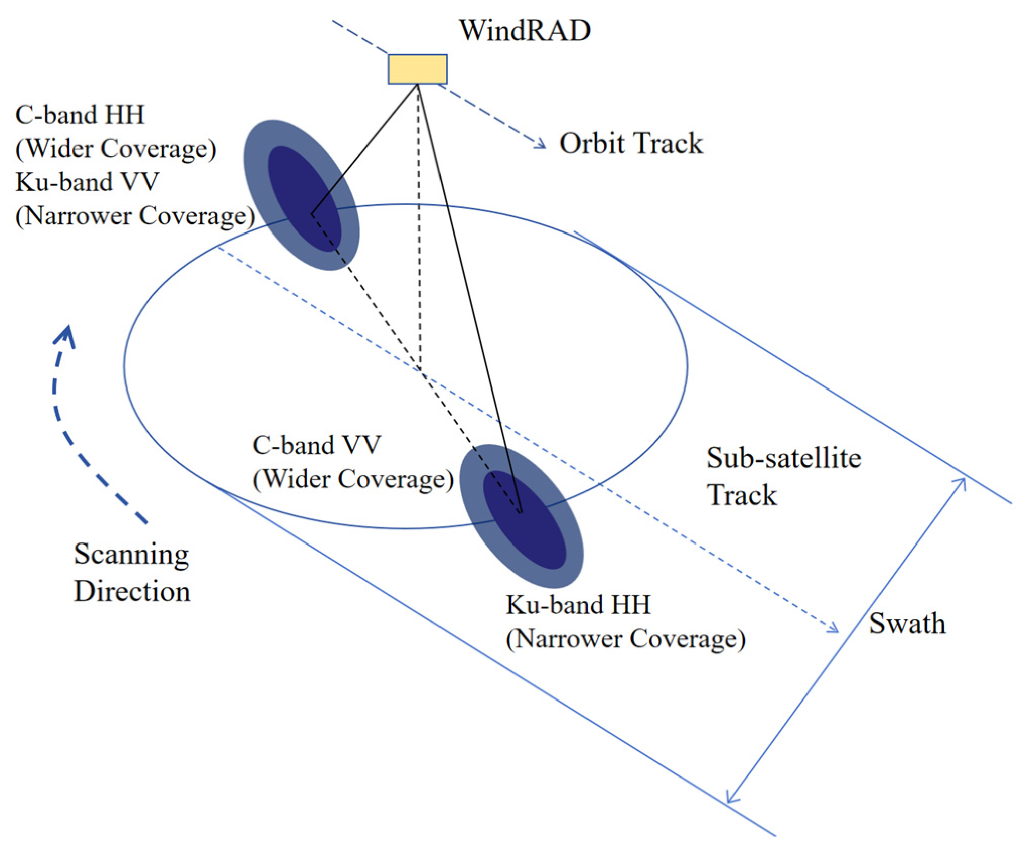
Figure 1. Measurement geometry of the WindRad antenna.
Remotesensing 17 02813 g001
Figure 2. Distribution of WVCs by number of views. The bar chart (left axis) indicates the number of WVCs with each specific view count. The yellow line (right axis) shows the cumulative proportion of total data covered by WVCs with view counts greater than or equal to the corresponding value.
Remotesensing 17 02813 g002
Figure 3. Distribution of ERA5 data. The blue histograms represent the frequency distributions of wind speed and direction, while the dark red boxplots illustrate the interquartile range and median values. The boxplot shown above displays the central 50% of the data (interquartile range), with the median line indicating the median value. Whiskers extend from the box to the minimum and maximum values of non-outlier data. (a) Statistical results for wind speed and (b) statistical results for wind direction.
Remotesensing 17 02813 g003
Figure 4. Scatter plots comparing TAO and ERA5 data: (a) scatter plot of u-component and (b) scatter plot of v-component.
Remotesensing 17 02813 g004
Figure 5. Schematic diagram of the neural network structure (taking a three-layer neural network as an example, including an input layer, one hidden layer, and an output layer).
Remotesensing 17 02813 g005
Figure 6. Density scatter plots of the retrieved u and v components using the model with the first set of hyperparameters and the second set of hyperparameters: (a) density scatter plot of the retrieved u component using the model with the first set of hyperparameters, (b) density scatter plot of the retrieved v component using the model with the first set of hyperparameters, (c) density scatter plot of the retrieved u component using the model with the second set of hyperparameters, and (d) density scatter plot of the retrieved v component using the model with the second set of hyperparameters.
Remotesensing 17 02813 g006
Figure 7. Density scatter plots of the retrieved u and v components using the model with the third set of hyperparameters and the fourth set of hyperparameters: (a) density scatter plot of the retrieved u component using the model with the third set of hyperparameters, (b) density scatter plot of the retrieved v component using the model with the third set of hyperparameters, (c) density scatter plot of the retrieved u component using the model with the fourth set of hyperparameters, and (d) density scatter plot of the retrieved v component using the model with the fourth set of hyperparameters.
Remotesensing 17 02813 g007
Figure 8. Density scatter plots of the retrieved wind components for the test dataset: (a) retrieved u component and (b) retrieved v component.
Remotesensing 17 02813 g008
Figure 9. Density scatter plot of wind speed. The horizontal axis represents the reference wind speed, while the vertical axis represents the retrieved wind speed.
Remotesensing 17 02813 g009
Figure 10. Distribution of absolute errors between retrieved and reference wind speeds across different wind speed ranges.
Remotesensing 17 02813 g010
Figure 11. Wind speed retrieval results for the test set (1 March 2024): (a) descending orbit and (b) ascending orbit.
Remotesensing 17 02813 g011aRemotesensing 17 02813 g011b
Figure 12. Wind speed maps over the study area on March 1, 2024: (a) ERA5 reference wind speed, (b) wind speed retrieved by the BP neural network, and (c) wind speed from the FY-3E satellite orbital product.
Remotesensing 17 02813 g012
Figure 13. Spatial distribution of wind speed RMSE on 1 March 2024: (a) retrieved wind speed by BP neural network and (b) wind speed from the WindRAD product.
Remotesensing 17 02813 g013
Figure 14. Scatter plot of wind direction retrieval on the training dataset.
Remotesensing 17 02813 g014
Figure 15. Box plot of deviations in different wind direction intervals.
Remotesensing 17 02813 g015
Figure 16. Wind direction distribution on the map: (a) reference wind direction, (b) retrieved wind direction, and (c) wind direction from WindRAD product.
Remotesensing 17 02813 g016
Figure 17. Spatial distribution of wind direction RMSE on 1 March 2024: (a) retrieved wind direction and (b) product wind direction.
Remotesensing 17 02813 g017
Figure 18. Scatter plots of wind speed comparisons: (a) BP neural network-retrieved wind speed versus TAO buoy observations and (b) FY-3E WindRAD product wind speed versus TAO buoy observations.
Remotesensing 17 02813 g018
Figure 19. Scatter plots of wind direction comparisons: (a) BP neural network-retrieved wind direction versus TAO buoy observations and (b) FY-3E WindRAD product wind direction versus TAO buoy observations.
Remotesensing 17 02813 g019
Table 1. Technical specifications of the wind field measurement radar.
ParameterSpecification for C BandSpecification for Ku Band
Spatial resolution25 × 0.5 km10 × 0.5 km
Swath width>1200 km
Scanning mode360° conical scanning
Minimum detectable wind speed3 m/s
(−26.2 dB)
3 m/s
(−30.8 dB)
Radiation resolution 10.5 dB (far end of swath, wind speed ≥ 5 m/s) 2
1.0 dB (far end of swath, wind speed = 3 m/s)
1 Providing data at a 25 km spatial sampling interval. 2 With a surface wind velocity of 5 m/s, the radar returns are recorded as −24.2 dB in the C-band and −25.5 dB in the Ku-band.
Table 2. Hyperparameter configurations used during training for different network structures.
Parameter
Combination
Hidden Layer Neuron CountActivation
Function
Layer 1Layer 2Layer 3
1512256128Leaky ReLU
2512256128Sigmoid
31024512256Leaky ReLU
41024512256Sigmoid
Table 3. The performance of the four hyperparameter combinations.
Parameter
Combination
RMSE for U Wind Component
(m/s)
R for U Wind ComponentRMSE for V Wind Component
(m/s)
R for V Wind Component
12.100.912.060.91
22.610.862.540.87
31.950.921.920.92
42.620.852.580.87
Table 4. Error across various wind speed groups.
Wind Speed RangeMean (m/s)Standard Deviation (m/s)
0–3 m/s1.071.24
3–6 m/s0.421.12
6–9 m/s0.060.99
9–12 m/s−0.421.09
12–15 m/s−1.141.30
>15 m/s−1.841.73
Table 5. Error across various wind direction groups.
Wind Direction RangeMean (°)Standard Deviation (°)
0–60°11.6122.54
60–120°0.0316.04
120–180°−10.5723.04
180–240°−6.5129.72
240–300°−0.2631.95
300–360°8.3724.29
Disclaimer/Publisher’s Note: The statements, opinions and data contained in all publications are solely those of the individual author(s) and contributor(s) and not of MDPI and/or the editor(s). MDPI and/or the editor(s) disclaim responsibility for any injury to people or property resulting from any ideas, methods, instructions or products referred to in the content.