Development of a Two-Stage Correction Framework for Satellite, Multi-Source Merged, and Reanalysis Precipitation Products Across the Huang-Huai-Hai Plain, China, During 2000–2020

Abstract

The acquisition of high-precision spatiotemporal precipitation data with long-term continuity plays an irreplaceable role in supporting agricultural modeling, hydrological forecasting, disaster prevention, and climate research. This study evaluates and corrects daily precipitation from satellite products (GPM, PERSIANN-CDR, CMORPH, GSMaP), merged datasets (GPCP, MSWEP, CHIRPS), and reanalysis products (ERA5, GLDAS) over the Huang-Huai-Hai Plain from 2000 to 2020. The study proposes a two-stage “error correction and residual correction” optimization framework. The error correction stage integrates machine learning with statistical methods (RF-DQDM), while the residual correction stage uses ground observations to dynamically adjust systematic biases. Results show that all corrected products outperform their original versions in spatial patterns and statistical metrics. Original precipitation data exhibit significant systematic errors modulated by topography, with eastern lowlands showing smaller errors. After correction, correlation coefficients rise above 0.8, and RMSE reductions average 60%. And product responses diverge significantly. CHIRPS improves from weakest to top performer, while model limitations constrain GLDAS enhancements. This framework establishes a transferable monsoon region optimization paradigm. This study provides a transferable bias correction framework for monsoon regions and builds a homogenized high-precision precipitation benchmark. It also recommends using CHIRPS or ERA5 for extreme rainfall analysis and MSWEP or GPCP for hydrological applications.

1. Introduction

Precipitation is a crucial component of water circulation [1]. Its spatiotemporal variations influence atmospheric circulation [2], and directly affect flood forecasting [3], drought warnings [4], and the accuracy of hydrological simulation [5]. Therefore, precipitation data with high-precision spatiotemporal resolution are crucial for hydrological simulation and water resource management [6]. The Huang-Huai-Hai Plain serves as China’s largest grain production base, supporting nearly 30% of the nation’s cultivated land and 40% of its grain output [7]. Accurate characterization of its precipitation’s spatiotemporal distribution is vital for maintaining agricultural irrigation efficiency and improving water resource management. However, precipitation in this region varies greatly between seasons and years. Summer often brings rainstorms, while droughts occur in winter and spring [8], which severely challenge traditional ground monitoring systems. Though considered the ‘gold standard’ for precipitation data, rain gauge stations in the Huang-Huai-Hai Plain face uneven distribution (especially in remote farmland) and spatial interpolation errors. This limits high-resolution data availability, failing to meet the requirements of precision agricultural hydrological models [9]. Under such circumstances, satellite products, multi-source merged products and reanalysis datasets have emerged as critical alternative data sources that leverage their high spatiotemporal coverage capabilities to compensate for the limitations of ground-based observations.

In recent years, bias correction has become a key technique in hydrometeorological research to improve the accuracy of satellite and climate model precipitation data. Traditional statistical methods, such as linear scaling, power transformation, and empirical quantile mapping (EQM), are widely used due to their simplicity and efficiency. However, these methods often fail in complex terrain, data-scarce regions, or when handling extreme precipitation events.

To address the limitations of traditional methods in handling extreme precipitation, Rohith and Cibin [10] proposed an extremes-weighted EQM (EW-EQM) method. This approach separates precipitation into extreme and non-extreme components, performs quantile correction for each, and applies weights to enhance the simulation of extremes. It effectively reduced extreme value errors (RMSE dropped from 12 mm to 6 mm) while preserving the ability of GCMs to project extreme trends. Building on this, machine learning methods have been increasingly applied to precipitation bias correction. Techniques such as Random Forest (RF) and Bidirectional Long Short-Term Memory (Bi-LSTM) networks have demonstrated strong performance in capturing complex nonlinear relationships and utilizing high-dimensional meteorological covariates. For example, YAO N et al. [11] enhanced a Bi-LSTM model with high-resolution meteorological variables from WRF simulations, significantly improving the correlation of hourly precipitation (CC increased from 0.43 to 0.60), thereby supporting extreme event simulation and real-time warning applications. In addition to improving model structures, researchers have also begun to focus on spatial heterogeneity and the integration of multi-source data. Linjiang Nan et al. [12] conducted a study in the Lancang River Basin and developed a two-stage framework combining sliding-window dynamic correction and Bayesian fusion. This approach significantly improved correction accuracy, with a monthly CC of up to 0.87, and enhanced the applicability of remote sensing data in regions with sparse ground observations. Spatial structural information has also become a key factor in improving correction accuracy. Meema et al. [13] proposed the ELM-ZB method, which integrates Extreme Learning Machines with climate zoning. By building correction models within climatically homogeneous regions, they achieved notable improvements in runoff simulation, with NSE increasing from 0.917 to 0.952. However, the method’s reliance on zonal consistency limits its generalizability to broader applications. To avoid reliance on real-time data and parameter assumptions, Gan et al. [14] proposed the DW method. It builds a historical bias probability distribution and corrects values using dry–wet season divisions and dynamic weighting. DW works well in overestimated regions, while quantile mapping (QM) remains effective in underestimated areas. In North America, bias correction methods such as QDM and SDM have been applied to adjust high-resolution climate projection data. QDM preserves the trend of simulated values and is well suited for median precipitation, while SDM uses Gamma distribution-based scaling and shows stronger capabilities in correcting extremes, reducing MAE by 85% at the 95th percentile. These methods demonstrate clear advantages on a daily scale and in extreme event simulations. Studies on ensemble strategies further indicate that the “correct-after-averaging” approach outperforms the “average-after-correcting” method, offering greater robustness in spatial distribution and extreme value correction [15].

Although existing studies have made important progress in improving the accuracy of precipitation data, several challenges remain. Current models often have limited generalization ability, making it difficult to handle the fusion of multi-source and multi-scale data. In addition, their capacity to identify residual errors is insufficient, limiting the ability to refine local systematic bias correction. Furthermore, inadequate treatment of spatial heterogeneity restricts regional adaptability and cross-regional transferability. To address the above limitations, this study proposes a two-stage hybrid bias correction framework combining error correction and residual adjustment, achieving three major breakthroughs. First, the correction mechanism innovates by coupling the dynamic feature learning ability of Random Forest (RF) with the statistical calibration strength of Dynamic Quantile Delta Mapping (DQDM). Unlike the static climate zoning used in ELM-ZB, RF-DQDM adaptively adjusts quantiles to avoid extrapolation errors at distribution tails (e.g., extreme rainfall events over 50 mm), thus overcoming ELM-ZB’s failure risk in mountainous areas. Second, the workflow design improves upon single-stage methods such as EW-EQM’s pointwise extreme value correction or the DW method’s one-step adjustment by adding a residual correction stage. This stage leverages gauge observations to dynamically reduce systematic bias. Third, the framework enhances applicability by overcoming the terrain simplification limitations of models like ELM-ZB, providing a transferable and robust solution suitable for complex monsoon regions [4].

Against this background, this study proposes a two-stage bias correction framework called “error correction and residual correction” for nine mainstream precipitation products over the Huang-Huai-Hai Plain from 2000 to 2020. These products include satellite datasets (GPM, PERSIANN-CDR, CMORPH, GSMaP), merged datasets (GPCP, MSWEP, CHIRPS), and reanalysis datasets (ERA5, GLDAS). The first stage employs a hybrid RF-DQDM model, combining the spatial feature learning ability of Random Forest (RF) with the statistical distribution calibration strength of Dynamic Quantile Delta Mapping (DQDM). The second stage builds a regression model based on residuals from ground gauge observations to dynamically correct systematic bias and enhance spatial consistency. Validation results show that this framework effectively reduces systematic errors and improves extreme precipitation simulation, providing technical support for regional hydrological modeling and climate risk assessment.

2. Materials and Methods

2.1. Study Area

The Huang-Huai-Hai Plain is situated between 109.75–124.94°E and 28.88–43.49°N, covering an area of ~400,000 km² (Figure 1). It is a crucial agricultural zone in central-eastern China, spanning the Yellow, Huai, and Hai River basins. Characterized by flat terrain (elevation mostly <50 m) and fertile soils, the Huang-Huai-Hai Plain serves as one of China’s primary grain production bases [16]. The region extends from north to south throughout the mild temperate, mesothermal, and subtropical zones. The annual rainfall is between 500 and 800 mm, with 60–70% of this precipitation occurring during the summer, though droughts occur frequently in winter and spring [17]. This region has large differences in precipitation over space and time. It also lies across several climate zones. These features make it a good area for evaluating precipitation products.

2.2. Datasets

Data from various datasets can be categorized into four types (

Table 1. Basic information on satellite, fused, and reanalysis precipitation products.

Products	Resolution		Coverage		Source
	Spatial	Temporal	Spatial	Temporal
Satellite products
GPM	0.1°	Monthly, Daily	Global	1998.1–2025.1	https://disc.gsfc.nasa.gov/datasets?keywords=IMERG&start=1920-01-01&end=2024-09-24&page=1 (accessed on 4 January 2025)
PERSIANN-CDR	0.25°	Monthly, Daily	60°S–60°N	1983–2024.10	https://www.ncei.noaa.gov/data/precipitation-persiann/access/ (accessed on 4 October 2024)
CMORPH	0.25°	Daily	60°S–60°N	1998–2024.8	https://rda.ucar.edu/datasets/d502002/dataaccess/ (accessed on 13 March 2025)
GSMaP	0.1°	Monthly, Daily	Global	1998.1–2025.7	https://sharaku.eorc.jaxa.jp/GSMaP/index.htm (accessed on 13 November 2024)
Multi-source merged products
GPCP	0.5°	Daily	Global	1998.1–2024.9	https://disc.gsfc.nasa.gov/datasets/GPCPDAY_3.3/summary?keywords=GPCP&start=1920-01-01&end=2024-09-24 (accessed on 28 February 2025)
MSWEP	0.1°	Monthly, Daily	Global	1979–2020	https://www.gloh2o.org/mswep/ (accessed on 22 November 2024)
CHIRPS	0.05°	Monthly, Daily	50°S–50°N	1981–2024	https://data.chc.ucsb.edu/products/CHIRPS-2.0/global_daily/ (accessed on 21 November 2024)
Reanalysis products
ERA5	0.1°	Monthly, Hourly	Global	1940–2025.7	https://cds.climate.copernicus.eu/datasets/reanalysis-era5-land?tab=overview (accessed on 21 May 2025)
GLDAS	1°	Monthly, Hourly	60°S–90°N	2000.1–2025.4	https://disc.gsfc.nasa.gov/datasets?keywords=GLDAS&start=1920-01-01&end=2024-09-24&page=1 (accessed on 1 December 2024)

). The first category comprises satellite precipitation products, which estimate precipitation parameters through spaceborne microwave/infrared sensors. These products enable global-scale monitoring with high spatiotemporal resolution [18]. In contrast, the second category consists of multi-source merged precipitation products. By integrating satellite observations, ground measurements, and model data through data assimilation and machine learning algorithms, these products achieve significant improvements in hydrological modeling accuracy [19]. The third group encompasses reanalysis precipitation products, which utilize numerical model assimilation and multi-source observations to generate physically consistent precipitation fields, particularly valuable for climate mechanism studies [20]. Finally, the fourth category involves conventional rain gauge data, providing a baseline truth for remote sensing product validation [21].

2.2.1. Satellite Precipitation Products

The Global Precipitation Measurement (GPM) core observatory satellite is a collaborative effort between the National Aeronautics and Space Administration (NASA) and the Japan Aerospace Exploration Agency (JAXA) [22]. As an extension and advancement of TRMM, the satellite employs high-precision precipitation monitoring to improve global hydrological cycle studies and disaster early warning capabilities [23]. GPM’s IMERG algorithm synthesizes multi-source microwave and infrared data to generate calibrated precipitation products classified into early, late, and final releases [24]. This study employs GPM’s Version 07 final precipitation datasets at monthly/daily resolutions to enable high-resolution climate analysis.

PERSIANN-CDR is a global precipitation database developed by the University of California, Irvine [25]. It uses neural networks to estimate rainfall by combining infrared data with historical precipitation data [26]. The algorithm dynamically adjusts weights to reduce errors. This dataset primarily sources geostationary satellite observations calibrated with GPCP products [27], offering continuous coverage from 1983 to present. It supports climate trend analysis and extreme event studies, especially in areas with limited ground observations.

CMORPH is a high-resolution precipitation dataset developed by the Climate Prediction Center (CPC) of the National Oceanic and Atmospheric Administration (NOAA) as part of the Climate Data Record (CDR) [28,29]. It applies a morphing motion vector technique to track cloud system movements. This method blends polar-orbiting satellite microwave data with geostationary satellite infrared observations. Motion vector interpolation fills observation gaps, enabling the effective detection of mesoscale convection like short-duration rainstorms [30]. The algorithm prioritizes microwave observations to minimize biases, using infrared data only as supplementary input.

GSMaP was developed by JAXA of Japan, which integrates GPM/REMM satellite data with geostationary observations using a microwave-infrared combined algorithm. Topographic correction and Kalman filter techniques enhance precipitation accuracy [31]. Its terrain-optimization module improves rainfall estimation in mountainous regions, while multi-satellite fusion enhances rainstorm monitoring over East Asia. The dataset includes versions like GSMaP-Gauge and GSMaP-MVK [32]. The study employs GSMaP-MVK V8 standard data with terrain-corrected G-suffix for spatiotemporal precipitation analysis.

2.2.2. Multi-Source Merged Precipitation Products

GPCP was developed by the World Climate Research Programme (WCRP) in collaboration with NASA, NOAA, and other agencies, combining satellite microwave/infrared data with global ground observations. Weighted averaging and systematic bias correction techniques optimize precipitation climate consistency, particularly enhancing accuracy in low-precipitation regions. The dataset integrates SSM/I satellite measurements and data from 6700 ground stations, forming a long-term climate record widely used in hydrological cycle studies and climate model validation [33]. This research utilizes GPCP Version 3.3, which incorporates multi-source satellite and ground-based data to support global precipitation analysis, climate monitoring, and model evaluation.

The MSWEP presents global historic precipitation data, developed by Utrecht University (the Netherlands) and Princeton University. MSWEP takes advantage of the complementary strengths of gauge-, satellite-, and reanalysis-based data for optimizing precipitation spatial patterns [34]. The methodology applies probability density functions to quantify multi-source uncertainties, reducing regional biases through weighted fusion [35]. This approach enhances precipitation interpolation accuracy in data-sparse regions by incorporating terrain elevation and vegetation coverage variables, significantly improving estimation robustness.

The CHIRPS is a quasi-global long-term precipitation dataset developed by the United States Geological Survey (USGS) and Climate Hazards Group (CHG) for drought monitoring. This dataset combines geostationary satellite (e.g., GOES) infrared cold cloud duration observations with ground measurements from 50,000 global stations, generating 0.05° high-resolution precipitation estimates through locally weighted regression [36]. Its innovation lies in leveraging the strong correlation between cold cloud persistence and precipitation probability, integrating historical climate data to establish region-specific models that enhance drought detection sensitivity [37]. While a hybrid approach addresses data gaps in ungauged areas, localized missing values persist even at high spatial resolutions.

2.2.3. Reanalysis Precipitation Products

The European Centre for Medium Range Weather Forecasts (ECMWF) released ERA5, a new reanalysis precipitation product, in 2017. ERA5 integrates multi-source data (satellite, radar) through a 4D-Var assimilation system. This reanalysis product uses coupled atmosphere–land–ocean models to optimize precipitation estimation with high resolution and physical consistency [38]. Its enhanced version of ERA5-Land achieves 0.1° spatial resolution by driving land surface simulations with the ERA5 atmospheric variable [39,40]. This study utilizes ERA5-Land daily precipitation data, accumulating them into monthly/annual series for high-accuracy land surface hydrology and climate analysis.

GLDAS is a global land data assimilation system jointly developed by the National Aeronautics and Space Administration (NASA) (https://www.sciencedirect.com/topics/agricultural-and-biological-sciences/national-aeronautics-and-space-administration (accessed on 1 December 2024)), Goddard Space Flight Center (GSFC), National Oceanic and Atmospheric Administration (NOAA), and the National Centers for Environmental Prediction (NCEP). The product integrates the Noah Land Surface Model with satellite observations (MODIS, GRACE) and ground-based measurements through data assimilation to optimize hydrological variables like soil moisture [41]. The system features a multi-layer soil temperature/moisture module and dynamic vegetation model, indirectly generating precipitation estimates coupled with surface hydrology [42]. GLDAS-2 includes three versions: 2.0 (Princeton meteorological forcing), 2.1 (model observation fusion), and 2.2 (with data assimilation) [43]. This study employs GLDAS Catchment Land Surface Model L4 V2.1 to achieve high-precision simulations of land surface hydrological processes.

2.2.4. Rain Gauge Data

The study selects observational data from 1052 rain gauge stations across the Huang-Huai-Hai region, covering the period from 2000 to 2020. The dataset encompasses daily/monthly precipitation measurements and station geographic coordinates. The climatic datasets were collected from the China Meteorological Administration (CMA, http://data.cma.cn/ (accessed on 3 November 2024)). These conventional observational records serve as real data measured at ground stations, providing a reliable benchmark for precipitation product evaluation. This ensures the accuracy and credibility of assessment outcomes.

In summary, this study selects precipitation products with comprehensive temporal coverage from 2000 to 2020, including IMERG-Final, PERSIANN-CDR, CMORPH, GSAMP/standard/V8, GPCP V3.3, MSWEP, CHIRPS, ERA5-Land, and GLDAS Catchment Land Surface Model L4. Regional cropping procedures are implemented to extract precipitation data specifically for the Huang-Huai-Hai region.

2.3. Methods

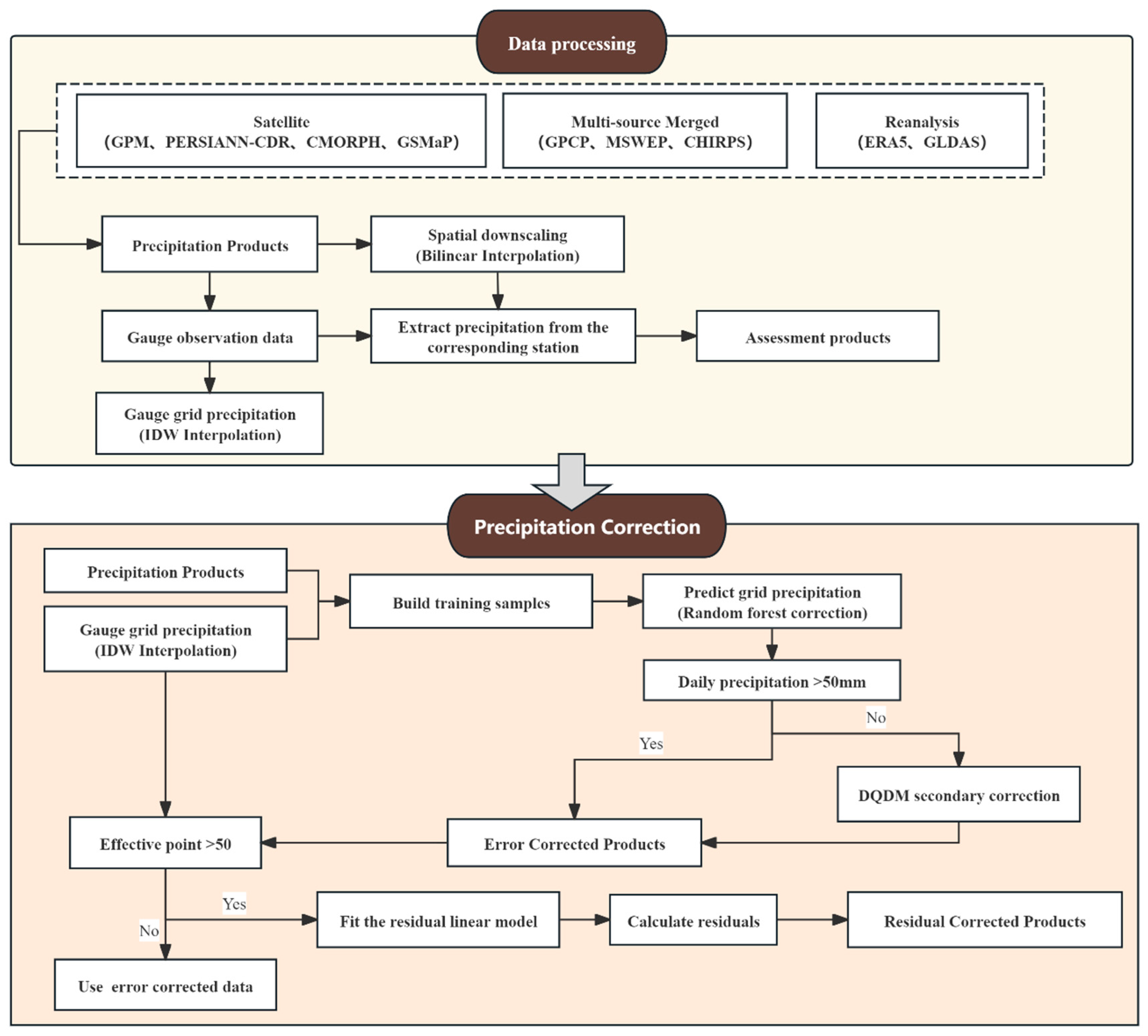
This study proposes a two-stage optimization framework for precipitation correction. The framework consists of error correction and residual correction, as shown in Figure 2. It aims to improve the accuracy and spatial consistency of satellite and reanalysis precipitation products, especially in regions with complex terrain.

2.3.1. Error Correction Stage: RF-DQDM

In the error correction stage, a multi-level correction method (RF-DQDM) that integrates machine learning and statistical mapping is applied to the precipitation products. As an ensemble learning algorithm, Random Forest (RF) [44] is an ensemble machine learning algorithm that builds multiple decision trees to improve model robustness and nonlinear prediction ability. In this study, the input features for the RF model include the raw precipitation product values and the station precipitation values interpolated using Inverse Distance Weighting (IDW). At each valid grid cell (where both inputs are available), a two-dimensional feature vector is created, and the interpolated station value is used as the target to train the model. To ensure reproducibility, the RF model uses the following hyperparameters: the number of trees (n_estimators) is 100, the maximum depth (max_depth) is set to none (allowing full tree growth), the bootstrap is enabled, and the random seed is set to 0. This configuration provides a balance between accuracy and stability.

After the RF prediction, Dynamic Quantile Delta Mapping (DQDM) [15,45] is used to adjust the statistical distribution. DQDM is a non-parametric mapping method that calibrates the predicted values by matching the empirical quantiles of the RF output to those of the interpolated station field. Specifically, for each grid cell, the quantile rank of the RF output is calculated and mapped to the same quantile in the target distribution. This step corrects distributional biases in the precipitation product. To avoid errors in extreme events, a bypass mechanism is applied. If the daily precipitation at any station exceeds 50 mm, the DQDM step is skipped, and the RF prediction is used directly. This threshold is chosen based on experience to avoid poor calibration in distribution tails caused by limited samples.

2.3.2. Residual Correction Stage: Statistical Bias Adjustment

This study further proposes a precipitation product residual correction method incorporating ground observations, which dynamically corrects systematic biases by establishing statistical relationships between satellite precipitation and ground observation residuals. Specifically, a linear regression model is constructed in regions where precipitation products and ground-interpolated fields have overlapping coverage [46]. This model takes the precipitation field from the first step (error correction) as the independent variable and the residual between ground observations and error-corrected product values as the dependent variable. Specifically, the residual between the bias-corrected product and the IDW-interpolated observation field is defined as follows:

$$\epsilon \left(i,j\right)=P_{obs}\left(i,j\right)-P_{RF\text{-}DQDM}\left(i,j\right)$$

(1)

where $P_{obs}\left(i,j\right)$ is the interpolated observation at the grid cell $\left(i,j\right)$, $P_{RF\text{-}DQDM}\left(i,j\right)$ is the bias-corrected precipitation from the first stage, $\epsilon \left(i,j\right)$ is the residual between the observation and the model estimate.

At the daily scale, for valid grid points (i.e., where both datasets are available), a linear regression model is established using $P_{RF\text{-}DQDM}$ as the independent variable and the residual $\epsilon$ as the dependent variable:

$$\epsilon \left(i,j\right)={\beta }_0+{\beta }_1{P}_{RF\text{-}DQDM}\left(i,j\right)+{\epsilon }_1$$

(2)

where ${\beta }_0$ and ${\beta }_1$ are regression coefficients, and ${\epsilon }_1$ is the stochastic error term of the regression model.

The final corrected precipitation is obtained by adding the predicted residual, as follows:

$$P_{final}\left(i,j\right)=P_{RF\text{-}DQDM}\left(i,j\right)+\widehat{\epsilon }\left(i,j\right)$$

(3)

where $\widehat{\epsilon }\left(i,j\right)$ is the predicted residual and the final corrected field $P_{final}\left(i,j\right)$ is obtained by adding the predicted residual to the bias-corrected field.

To ensure stable regression, the model is only applied when the number of valid grid cells is at least 50. This threshold avoids overfitting and ensures sufficient sample size for reliable estimation. It was chosen based on sensitivity analysis.

This two-stage framework has both flexibility and effectiveness. It integrates observation data and satellite products and combines machine learning with statistical modeling. However, there are still some limitations. RF does not model spatial patterns explicitly and may produce noise in local regions. DQDM depends on the representativeness of the sample distribution and may perform poorly in heavy rainfall events due to limited data. The residual correction uses a simple global linear model and does not include spatial covariates. Future improvements may consider geographically weighted regression (GWR) or regional segmentation. The performance of the RF model can also be influenced by the choice of hyperparameters. Parameter tuning may be needed when applying the method to other regions.

In summary, the two-stage correction method improves precipitation accuracy. It performs well under complex terrain and extreme weather conditions and provides a practical approach for hydrological modeling and climate analysis.

3. Results

3.1. Precipitation Analysis

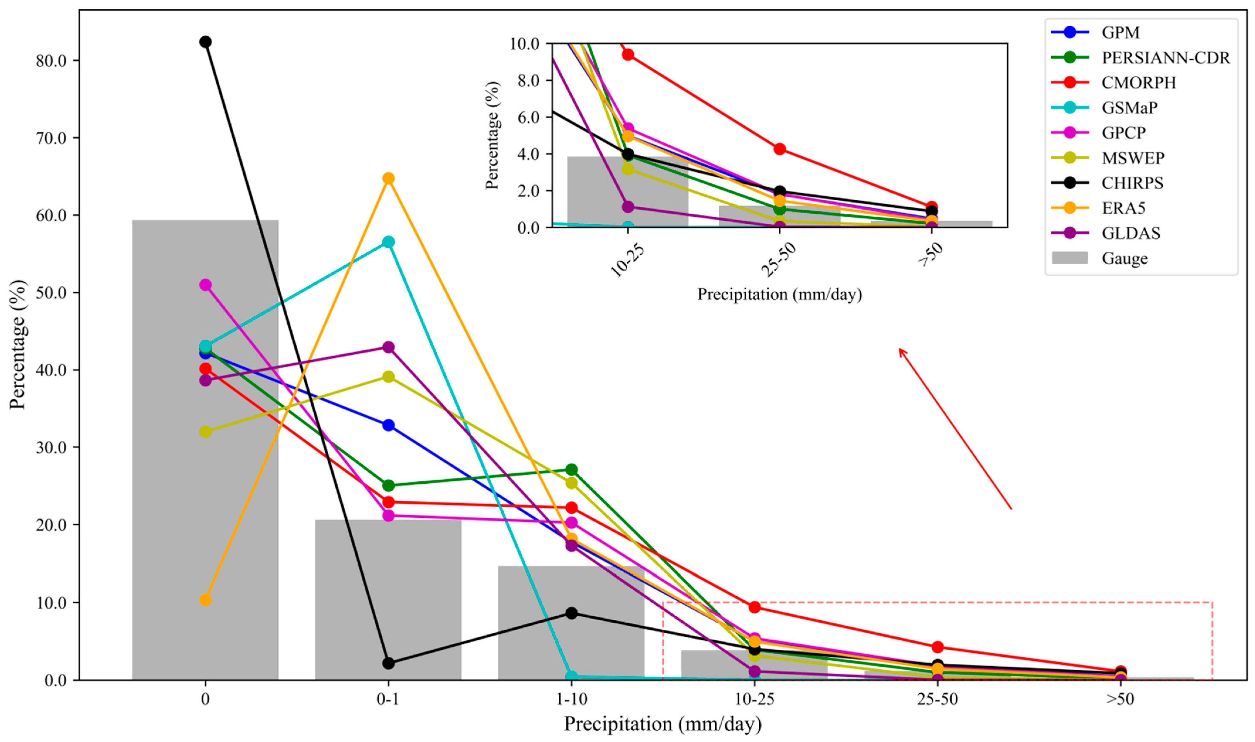
The Chinese meteorological standard [9] classifies the daily precipitation into six types, including non-rainfall (with zero precipitation), slight precipitation (with a daily precipitation amount between 0 and 1 mm/day), small precipitation (with a daily precipitation amount between 1 and 10 mm/day), moderate precipitation (with a daily precipitation amount between 10 and 25 mm/day), heavy precipitation (with a daily precipitation amount between 25 and 50 mm/day), and extreme precipitation (with a daily precipitation amount >50 mm/day). In this study, the original precipitation data of precipitation products were statistically classified. The precipitation frequency distribution analysis based on Figure 3 reveals that most products systematically underestimate non-rainfall event frequencies, with CHIRPS being the sole exception, demonstrating significant overestimation. In slight and small precipitation intensities, CHIRPS exhibits underreporting while other products generally overestimate occurrence rates. For moderate and heavy precipitation categories, PERSIANN-CDR, MSWEP, and ERA5 show higher consistency with the observations, whereas the remaining products overestimate frequencies. In extreme precipitation detection, ERA5 demonstrated superior accuracy, contrasting with CHIRPS’ pronounced overestimation. The results indicate that the products have difficulty accurately capturing short-duration heavy precipitation and require further correction.

To further elucidate error sources, this study employs the error decomposition model proposed by AghaKouchak et al. [47], which dissects total error into systematic error and random error [48]. Through error decomposition techniques, systematic errors can be mitigated through regression correction driven by ground-based observations, while the suppression of random errors requires multi-source data fusion or spatiotemporal smoothing algorithms [49]. Moreover, the spatial distributions of the error components with regard to systematic and random errors in nine precipitation products across the Huang-Huai-Hai Plain are presented in Figure 4. Understanding these error components is essential before applying any statistical adjustments to integrate these products into specific applications [50]. Overall, except for CHIRPS, all products exhibit a systematic error contribution exceeding 50%. Notably, GSMaP and GLDAS show a dominant systematic error contribution of up to 90% across the entire plain, which is related to the simplification of cloud microphysics in satellite retrieval algorithms and uncertainties in land–atmosphere coupling in reanalysis models. However, GPM and CMORPH display similar contributions from systematic and random errors, with no significant difference. CHIRPS stands out with a systematic error contribution below 35%, lower than its random error contribution. This is mainly due to its gauge-based bias correction, which reduces systematic bias. Spatially, systematic errors are generally lower in the eastern lowland areas of the plain than in the western highlands, with PERSIANN-CDR showing the most pronounced spatial variability. This supports the widely accepted view that topographic complexity negatively impacts precipitation retrieval accuracy. Flat terrain reduces microwave/infrared signal attenuation, and a stable monsoon climate lowers precipitation heterogeneity in time and space, thereby minimizing model-related spatial errors. In response to these findings, this study applied both error correction and residual correction to all precipitation products to enhance their spatiotemporal accuracy and mitigate the influence of different types of errors.

3.2. Precipitation Correction

In this study, a spatial matching validation framework is established by integrating rain gauge data with multi-source precipitation products, employing point-to-pixel analysis to systematically evaluate product accuracy [51]. Following the geospatial alignment principle, gridded precipitation data are spatially overlaid with station measurements, where bilinear interpolation extracts precipitation estimates at gauge locations. The performance of precipitation products was quantitatively analyzed with respect to five evaluation metrics (

Table 2. Relevant information on continuous and categorical statistical indicators.

Scores	Equation	Perfect Value
Bias	$Bias={\displaystyle \frac{{\displaystyle {\sum }_{i=1}^N(S_i-G_i)}}{{\displaystyle {\sum }_{i=1}^N{G}_i}}}$	0
CC	$CC={\displaystyle \frac{{\displaystyle {\sum }_{i=1}^N(S_i-\overline{S})(G_i-\overline{G})}}{\sqrt{{\displaystyle {\sum }_{i=1}^N{(G_i-\overline{G})}^2}}\sqrt{{\displaystyle {\sum }_{i=1}^N{(S_i-\overline{S})}^2}}}}$	1
RMSE	$RMSE=\sqrt{{\displaystyle \frac{1}{N}}{\displaystyle {\sum }_{i=1}^N{(S_i-G_i)}^2}}$	0
KGE	$KGE=1-\sqrt{{(CC-1)}^2+{(\overline{S}/\overline{G}-1)}^2+{(C{V}_S/C{V}_G-1)}^2}$	1
CSI	$CSI={\displaystyle \frac{H}{H+M+F}}$	1
Random Err.	$RandomErr.=\sqrt{{\displaystyle \frac{{\displaystyle {\sum }_{i=1}^N{(S_i-S_i^{*})}^2}}{N}}}/RMSE$
System Err.	$SystemErr.=\sqrt{{\displaystyle \frac{{\displaystyle {\sum }_{i=1}^N{(S_i^{*}-G_i)}^2}}{N}}}/RMSE$
With $S_i^{*}$,	$S_i^{*}=a\times G_i+b$
With $S_i$, $G_i$	$S_i$—precipitation for products; $G_i$—precipitation for the station observation data

). Bias is the overall deviation of SPPEs from gauge observations [52]; CC employs Pearson’s linear correlation analysis to reveal trend consistency between precipitation products and observational data [53,54]; RMSE amplifies error contributions from heavy precipitation events through quadratic computation, demonstrating heightened sensitivity to estimation biases in rainstorms episodes [55,56]; and the KGE serves as a comprehensive evaluation metric designed to harmonize the balanced contributions of the correlation coefficient, mean deviation, and dispersion deviation in assessing hydrological model performance [57,58]. The critical success index (CSI) demonstrates enhanced robustness in heavy precipitation detection assessments by balancing missed detection and false alarm effects [59,60].

3.2.1. Comparison of Evaluation Metrics

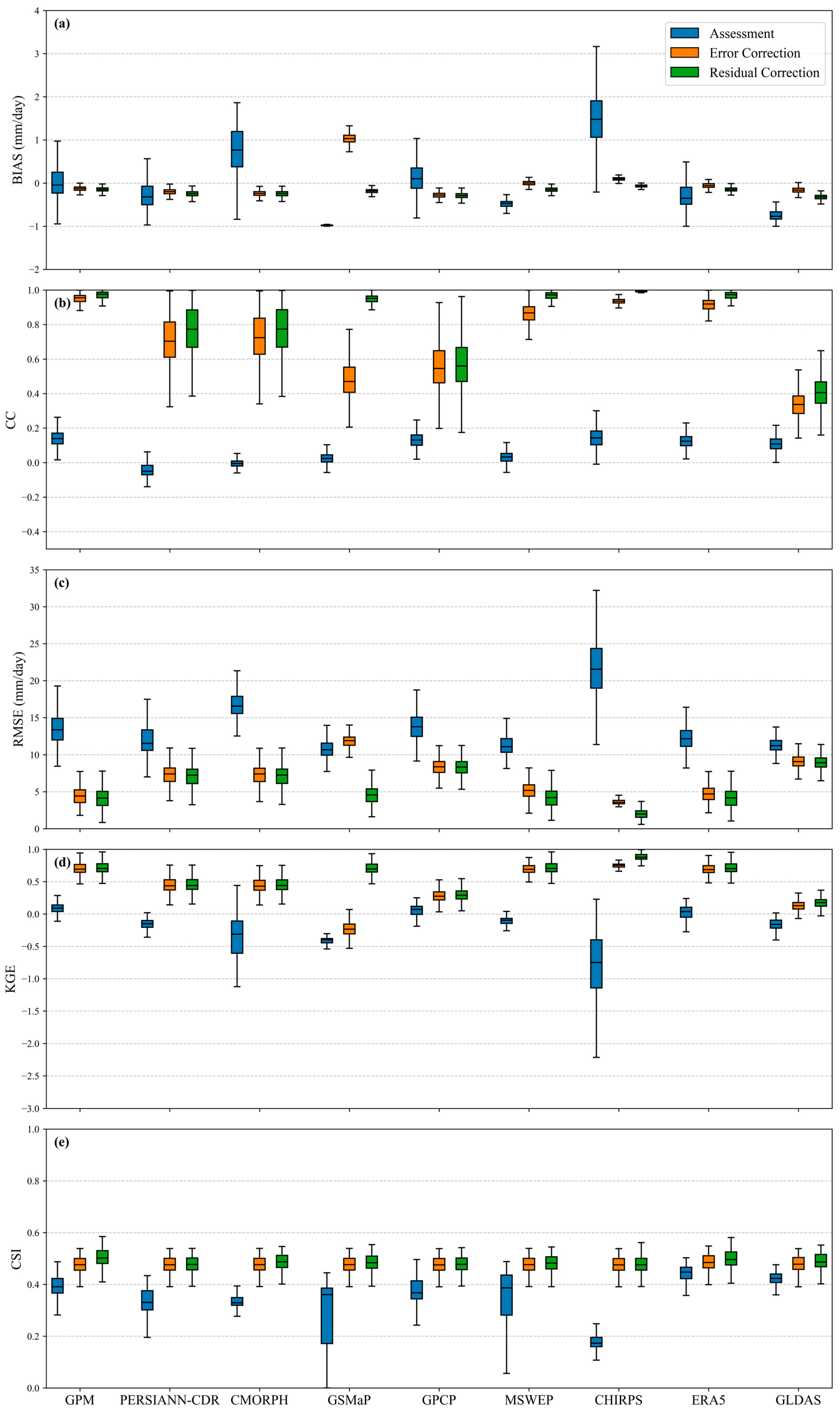
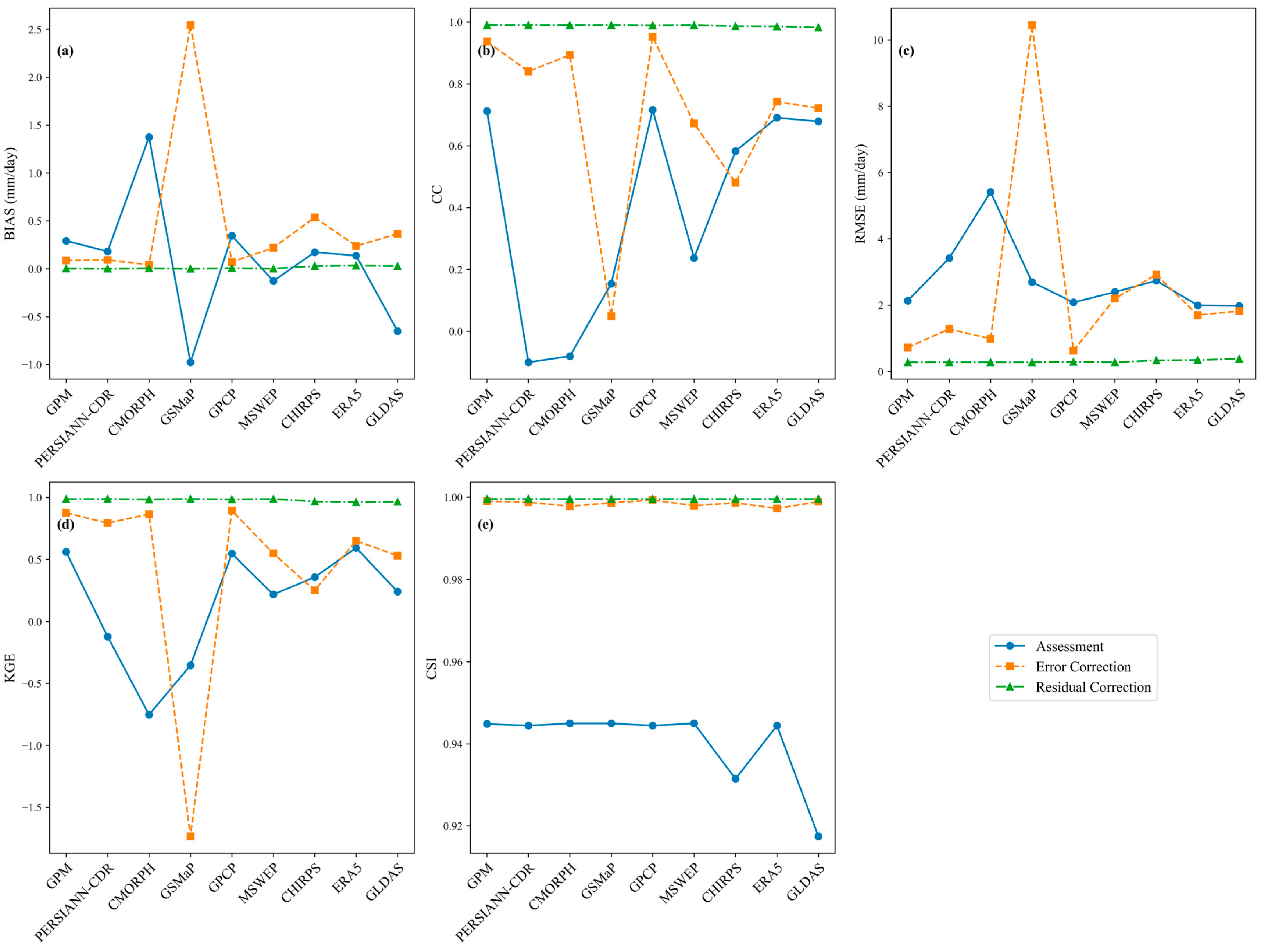
Figure 5 provides a comprehensive comparison of the overall performance of the products before and after correction, showing that error correction with residual correction significantly improves the accuracy. Without correction, CHIRPS is significantly overestimated (bias = 1.65 mm/day), GSMaP is significantly underestimated (−0.98 mm/day), and the deviation of the rest of the products is in the range of −0.5 mm/day–0.5 mm/day, and the absolute value of bias of most of the products converges to <0.3 mm/day after error correction. The systematic deviation after residual correction further converges to zero, such as CHIRPS, which decreases from 0.09 to −0.08 after correction, and GSMaP, which reverses from 1.01 to −0.20. CC improved from weak initial correlations to strong correlations, generally around 0.6. After residual correction, CHIRPS reached 0.987, and both ERA5 and GPM exceeded 0.947. Only GLDAS remained relatively low (0.389), indicating the limitations of reanalysis data in capturing dynamic precipitation processes. RMSE decreased by about 60% overall, with CHIRPS being the most prominent, going from uncorrected 23.23 mm/day to error-corrected 3.81 mm/day to residual-corrected 2.37 mm/day, and, finally, all products had RMSE < 10 mm/day. The KGE efficiency coefficients move from generally negative to strongly positive, residual corrected CHIRPS (0.82) and ERA5 (0.62) are the best performers, the CSI indices increase across the board, ERA5 is always in the lead, going from an uncorrected 0.41 to a residual-corrected 0.46, and CHIRPS showed the largest relative improvement of about 147%, indicating a successful transformation from the weakest to one of the most competitive products.

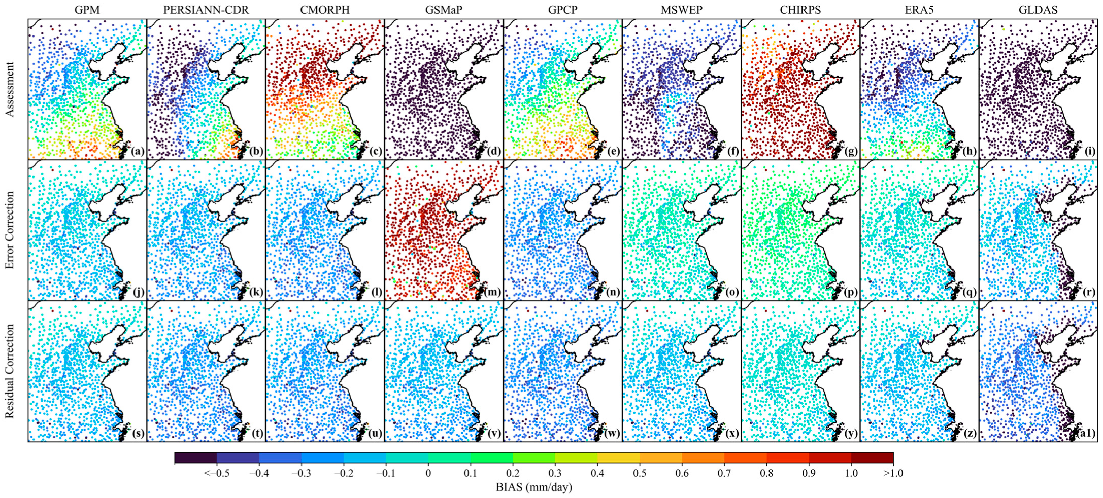
The boxplots in Figure 6 and the spatial maps in Figure 7, Figure 8, Figure 9, Figure 10 and Figure 11 intuitively illustrate the spatial variability and distribution of evaluation metrics at individual stations. Among the original precipitation products, only GPM, PERSIANN-CDR, MSWEP, and ERA5 had more than 60% of samples with absolute error values within 0.1 mm/day. In contrast, GSMaP and CHIRPS had less than 0.1% of samples meeting this criterion, with CHIRPS showing particularly poor performance—77.41% of its samples had errors greater than 1 mm/day. After applying error correction, the proportion of samples with absolute errors within 0.1 mm/day exceeded 96% for most products. However, GSMaP remained an outlier, with only 2.36% of its samples meeting the threshold, and most of its errors exceeding 0.5 mm/day. Following residual correction, all products had only one remaining sample with an error greater than 1 mm/day, located in the upper-left highland region of the Huang-Huai-Hai Plain. For all products except GLDAS, most samples had absolute errors within 0.1 mm/day. For GLDAS, only 78.68% of samples fell within this range (Figure 6a and Figure 7).

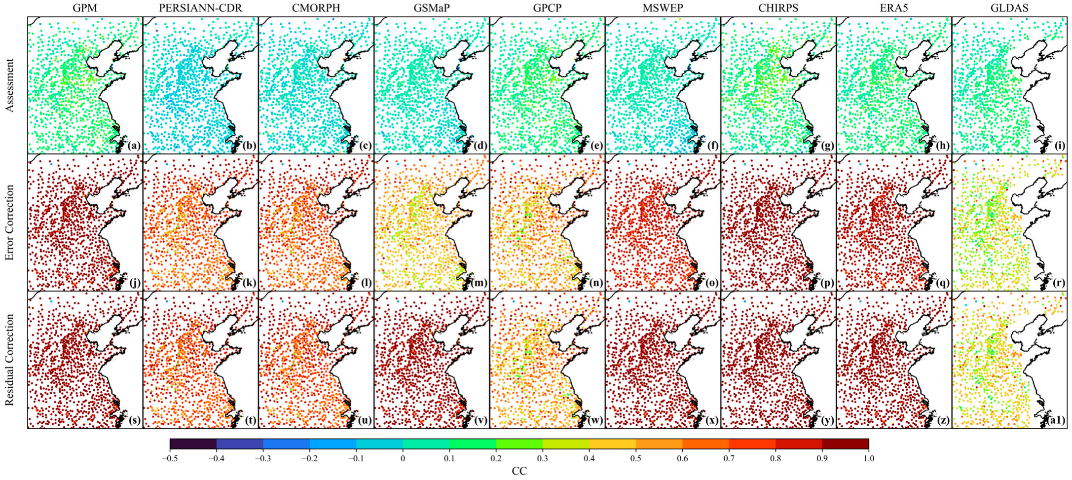
Figure 6b and Figure 8 show that the correction process significantly improves the product correlation. The original data show severe negative correlation, with CC < 0 for up to 82.91% of the samples for PERSIANN-CDR, 59.23% for CMORPH, about 20% for GSMaP and MSWEP, and over 99% of the samples for all the products have a CC < 0.5. After error correction, negative correlations were largely eliminated. For example, the negative correlation samples of both PERSIANN-CDR and CMORPH plummeted to 0.20%. Weak correlations (CC < 0.5) were significantly replaced by strong correlations (CC > 0.5), and more than 90% of samples for most products had CC > 0.5. Only GSMaP (39.19%) and GLDAS (7.8%) remained dominated by weak correlations. In the residual correction stage, strong correlations dominate across all products. More than 95% of samples showed strong correlations for most precipitation datasets. However, GPCP (66.40%) and GLDAS (only 18.76%) are relatively lagging in performance.

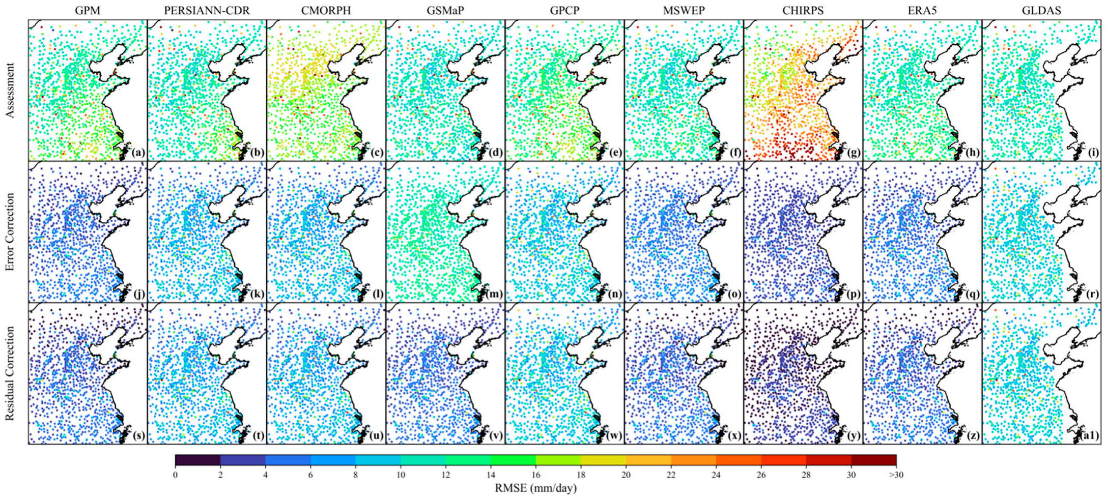
Figure 6c and Figure 9 reveal the significant improvement in error performance. Before correction, high errors were prominent. For example, 66.16% of CHIRPS samples had RMSE values greater than 20 mm/day, and GSMaP had 3.93% in this range. Only a few products, such as GSMaP and MSWEP, had more than 10% of their samples in the low error range (<10 mm/day). Error correction greatly improved this situation. Extreme high errors (>20 mm/day) were nearly eliminated—for instance, CHIRPS dropped to 0%, and GSMaP to 0.69%. For all products, the proportion of samples in this range was reduced to below 1.71%. The dominance of low error samples increased significantly. GPM, MSWEP, and ERA5 all rose to around 97% in this range, and CHIRPS showed a dramatic improvement from just 0.30% to 99.60%. The subsequent residual correction further enhanced accuracy. A total of 7/9 products have more than 97% of <10 mm/day, with CHIRPS, ERA5, and MSWEP exceeding 99.60%. However, GLDAS still had 20.21% of samples in the medium-error range (10–20 mm/day), with only 78.08% in the <10 mm/day range.

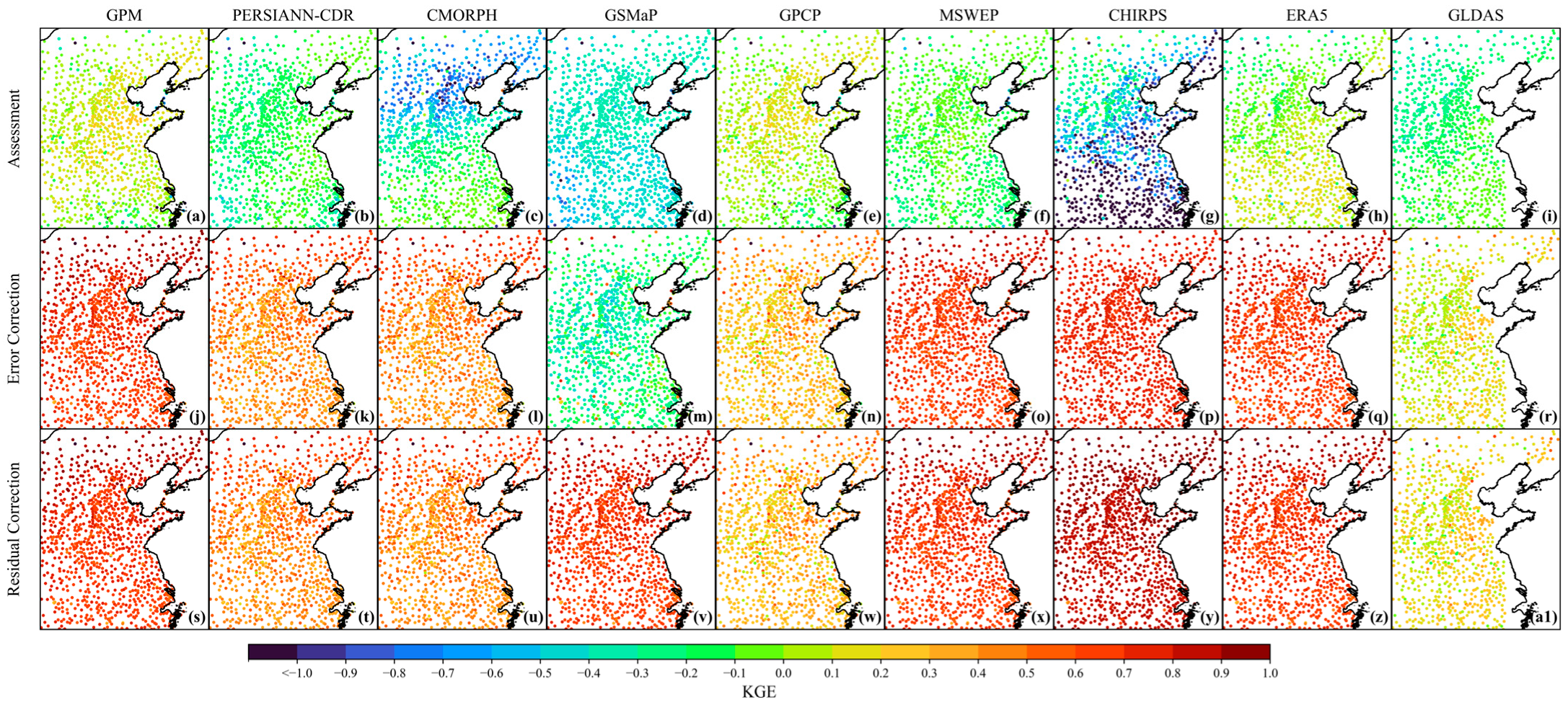
Figure 6d and Figure 10 exhibit the evolution of the efficiency coefficients. The initial assessment of the uncorrected reveals severe inefficiencies, with PERSIANN-CDR, GSMaP, and GLDAS having a KGE < 0 for nearly 100% of the samples, and only performs relatively better (only 19.47% < 0). All products had 100% of samples with KGE < 0.5. Error correction brought a fundamental shift. Negative efficiency was nearly eliminated, with all products having less than 1.96% of samples with KGE < 0. The high-efficiency range (>0.5) expanded greatly. For example, GSMaP jumped from 100% < 0 to 96.37% > 0.5, and CHIRPS from 98.79% < 0 to 99.39% > 0.5. However, PERSIANN-CDR and CMORPH were still dominated by medium efficiency, with about 68% of their samples below 0.5, and GLDAS had 99.39% < 0.5. After residual correction, high efficiency (>0.5) became dominant. GPM, MSWEP, CHIRPS, and ERA5 had over 96% of samples in this range, and GSMaP maintained a high level at 96.37%. PERSIANN-CDR and CMORPH still had about 66% of samples in the moderate efficiency range, and even after correction, 98.54% of GLDAS samples remained below 0.5.

Figure 6e and Figure 11 document the trajectory of CSI improvement. In the uncorrected phase, most products had a high proportion of low CSI values (<0.2), especially CHIRPS (78.88%) and GSMaP (27.95%). Only MSWEP and ERA5 had more than 15% of samples with CSI > 0.45. Error correction effectively alleviated this issue. The proportion of low CSI intervals is reduced, with CHIRPS plummeting from 78.88% to 6.48% and GSMaP from 27.95% to 8.17%. The middle and high CSI range expanded, and the proportion of samples with CSI > 0.45 generally rose above 70% (e.g., CMORPH and GSMaP reached 70.34%), and ERA5 is leading the way with 76.98%. The final residual correction further enhanced performance. High CSI values (>0.45) continued to improve, with ERA5 increased to 83.14%, a 39.37% improvement over the uncorrected version. Satellite products like GPM and MSWEP exceeded 75%. Low CSI samples (<0.2) were almost entirely eliminated, with all products reduced to below 8.17%, and CHIRPS further dropping to 6.48%.

3.2.2. Areal Precipitation Analysis

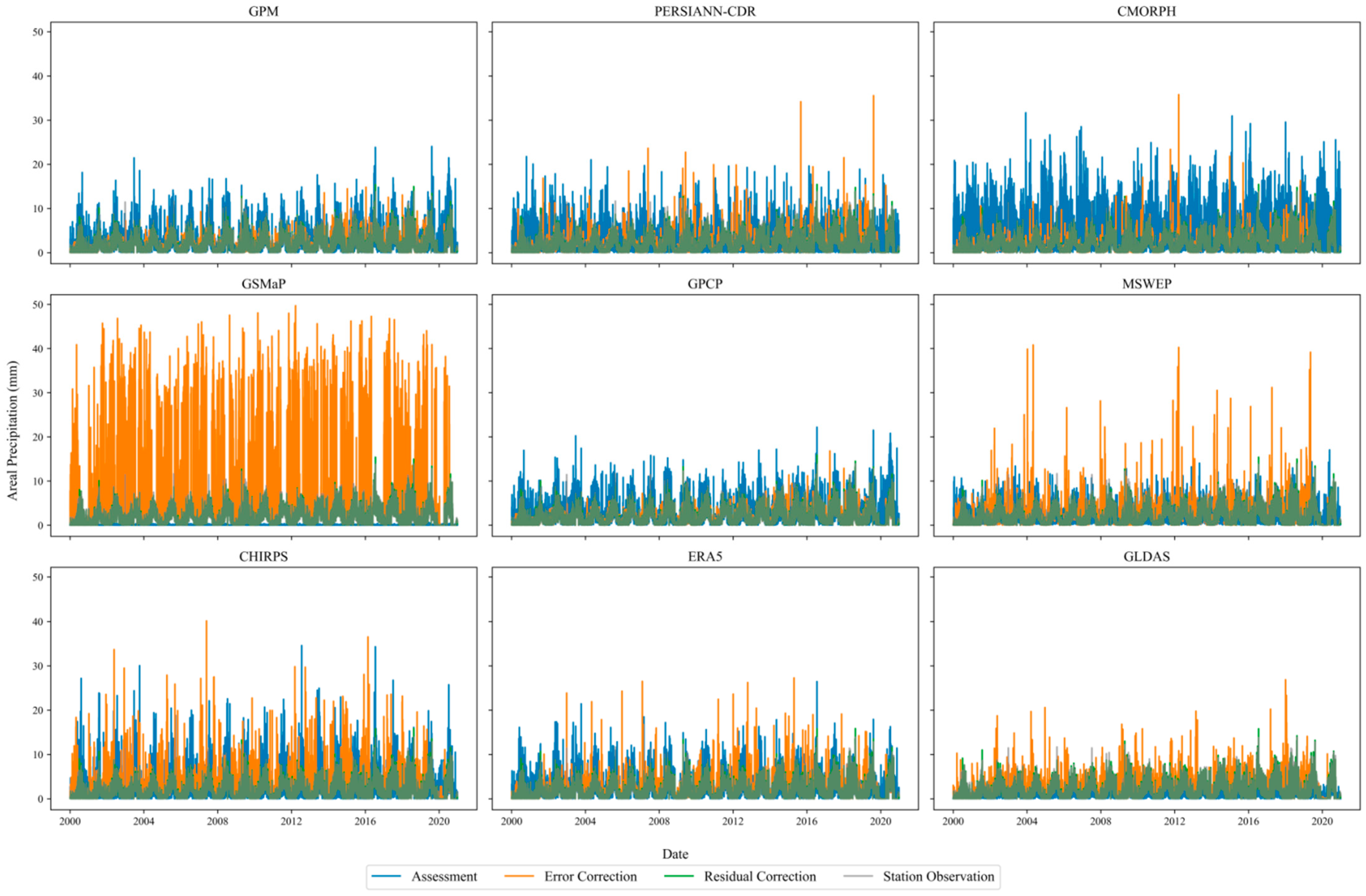
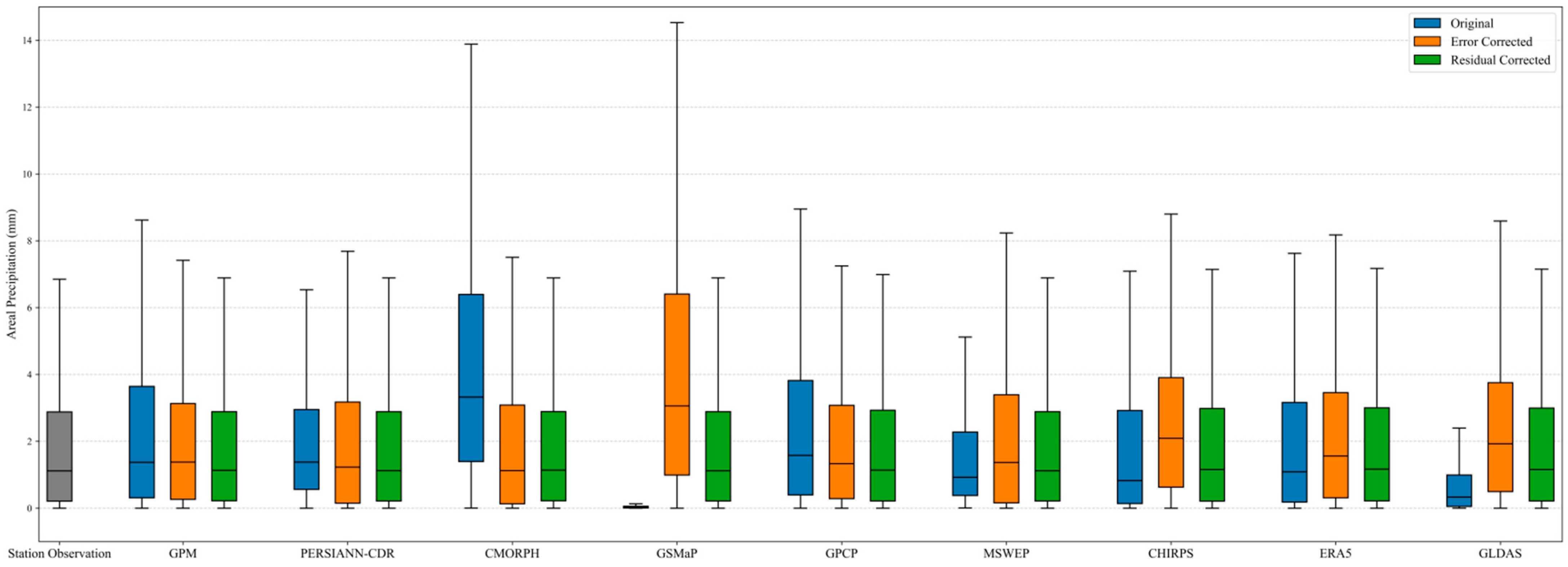
In this study, areal precipitation was calculated for both station observations and all precipitation products, and the results were evaluated accordingly. Given the sparse distribution of stations, the Thiessen polygon method was used to calculate areal precipitation from station data. Figure 12 and Figure 13 illustrate the daily areal precipitation trends from stations and each product during 2000–2020, before and after correction.

Based on the evaluation using station-based areal precipitation as a reference, the results show a systematic improvement in product performance through a stepwise optimization process: original data → error correction → residual correction. In the original stage, significant biases were common. CMORPH showed a strong positive bias (1.375 mm), with areal precipitation generally higher than that of stations; and GSMaP showed a large negative bias (−0.976 mm), with areal values significantly lower than station values. Although GLDAS had the lowest RMSE (1.975 mm), it still showed a negative bias (−0.651 mm), low efficiency (KGE = 0.242), and weak correlation (low CC). Correlation was generally poor, with PERSIANN-CDR and CMORPH even showing negative correlation; and the highest CCs were for ERA5 (0.691) and GPCP (0.716), but neither exceeded 0.72. Despite this, event detection ability was relatively good. All products had CSI values greater than 0.93, indicating a basic capacity to identify precipitation events.

After error correction, most products’ areal precipitation moved closer to station values, with bias ≤ 0.24 mm, except for the GSMaP anomaly of 2.544 mm, and the surface rainfall is significantly higher than the site surface rainfall. Correlation improved markedly, with most products achieving CC > 0.5, and GPCP performed best (CC = 0.952) (Figure 14). However, GSMaP correlation collapsed (CC = 0.049). The error performance is differentiated, with some products (e.g., GPCP) achieving low error (RMSE = 0.624 mm), while the RMSE of GSMaP and CHIRPS is still greater than 2 mm. Event detection remained excellent, with all products reaching CSI > 0.99. Further analysis revealed that the RF-DQDM method achieved notable improvements for CHIRPS but had negative effects on GSMaP. This divergence mainly stems from differences in the characteristics of the original data. CHIRPS integrates ground observations with a relatively stable error structure. RF can model its systematic bias well, and DQDM effectively improves its extreme precipitation and spatial consistency. In contrast, GSMaP relies on satellite retrievals, which have non-stationary, high-frequency errors. RF struggles to model these errors accurately, and DQDM fails to map their distribution properly, potentially amplifying noise and reducing accuracy. These results suggest that bias correction is not universally effective across all precipitation products. Calibration strategies should be tailored to the specific characteristics of each data source.

Residual correction brought a fundamental breakthrough. Areal precipitation values matched station data very closely. Relative biases were near zero. Correlation coefficients were all above 0.98. RMSE values dropped below 0.5 mm. Event detection rates (CSI > 0.99) and overall efficiency (KGE > 0.96) approached theoretical optimal levels. This process overcomes the inherent differences among multiple data sources and achieves consistency and homogenization of areal precipitation. It provides a reliable foundation for driving subsequent hydrological models.

3.2.3. Uncertainty Analysis

As a robust approach to evaluating the relative uncertainty of products without any prior knowledge of the true sequence, building on experience from assessing ET products, the Triple Collocation (TCH) method can be employed to quantify precipitation product uncertainty [61,62]. This method resolves the absence of true reference sequences by establishing a mathematical framework of relative errors derived from triple product combinations and relative error calculations of reference sequences.

The sequence of each product was defined as ${\left\{X_{\dot{i}}\right\}}_{i=1,2,\cdots ,N}$, as follows:

$$X_i=X_t+{\epsilon }_i,\forall i=1,2,\cdots N$$

(4)

where $X_{\dot{i}}$ is the simulated value of the product; $X_t$ is the true time series; ${\epsilon }_i$ is the error term; and N is the total number of products (in this study, N = 9). TCH addresses the absence of the true sequence by calculating the relative error of the products and the reference sequence, as follows:

$$Y_i=X_i+X_{ref}={\epsilon }_i-{\epsilon }_{ref},\forall i=1,2,\cdots N-1$$

(5)

where $Y_i$ is the relative error and $X_{ref}$ is the reference sequence, selected from the products. The covariance matrix (S) of Y is expressed as follows:

$$S=Cov\left(Y\right)$$

(6)

Upon introducing an N × N noise covariance matrix (R) with principal diagonal elements representing the squared uncertainties of each sequence, and an auxiliary matrix (J), the relationship between the S and R matrices can be defined as follows:

$$S=J\cdot R\cdot J^T$$

(7)

By combining these matrices, the elements in matrix R are deduced as follows:

$$r_{ij}=s_{ij}-r_{NN}+r_{\dot{i}N}+r_{jN}$$

(8)

The uncertainty (δ) of each sequence is represented by the square root of the principal diagonal elements in R.

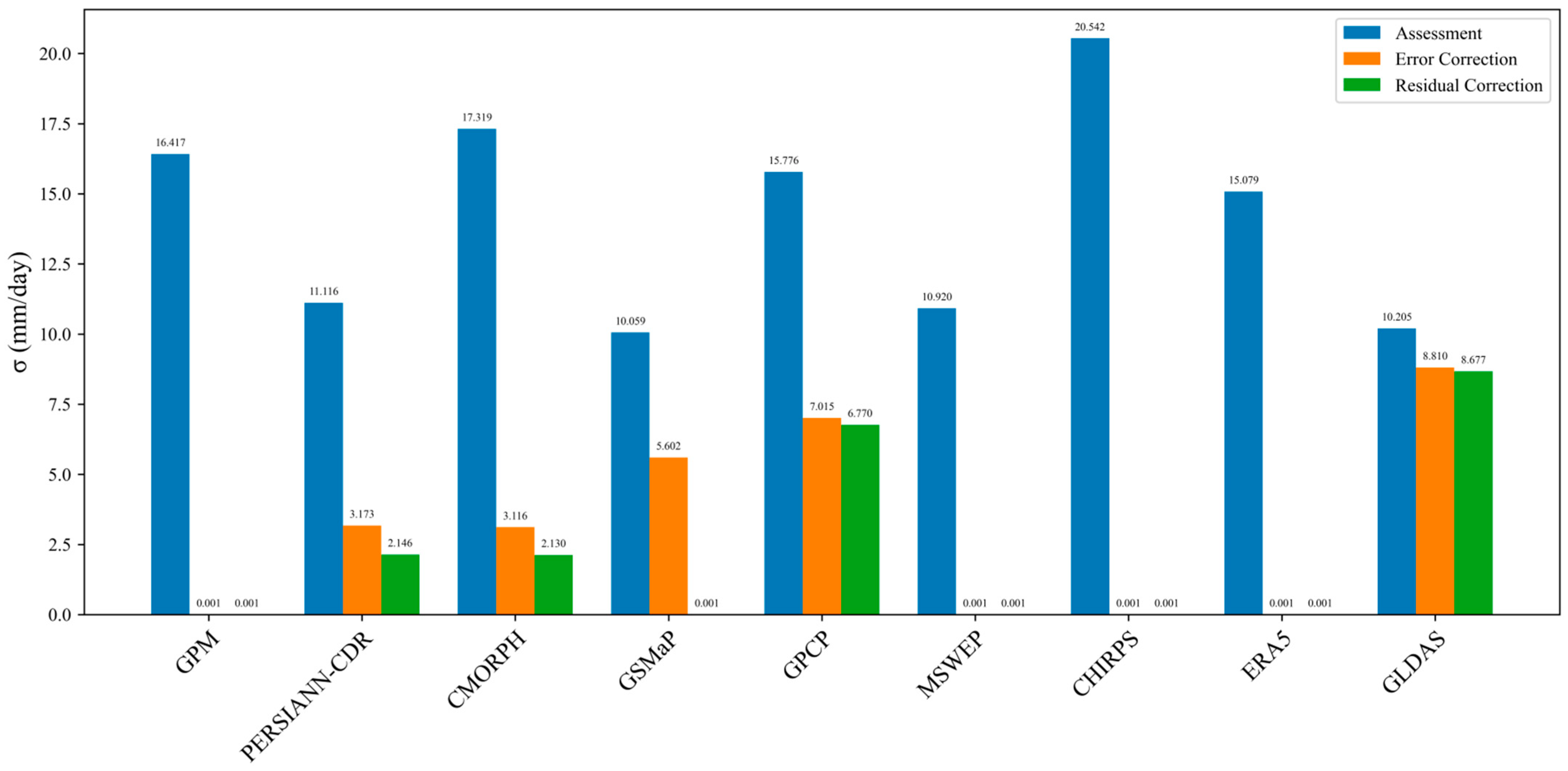
Figure 15 illustrates the evolution of precipitation product uncertainty along the optimization pathway from “uncorrected → error correction → residual correction” during the period of 2000–2020. In the uncorrected stage, all products exhibited high uncertainty levels (>10 mm/day). Among them, CHIRPS had the highest uncertainty at 20.54 mm/day, while GSMaP showed the lowest at 10.06 mm/day. After error correction, uncertainties decreased significantly and began to diverge across products. GPM, MSWEP, CHIRPS, and ERA5 quickly dropped to levels close to the theoretical lower limit. Single satellite algorithm products such as PERSIANN-CDR and CMORPH showed some improvement but remained in the range of 3.12–3.17 mm/day. Reanalysis products lagged behind, with GPCP reduced to 7.01 mm/day and GLDAS to 8.81 mm/day. In the residual correction stage, uncertainty patterns improved further. GSMaP successfully converged to near-theoretical minimum values. PERSIANN-CDR and CMORPH continued to improve, reaching 2.13–2.15 mm/day. However, GPCP (6.77 mm/day) and GLDAS (8.68 mm/day) remained at high uncertainty levels and failed to achieve significant breakthroughs. This figure clearly demonstrates the universal effectiveness of the correction framework in reducing uncertainty across multi-source precipitation datasets, while also highlighting the varying responses and final convergence levels of different algorithm types during the correction process.

4. Discussion

This study applied a multilevel error correction method for precipitation products (RF-DQDM). It combines machine learning and statistical mapping and a residual correction method for precipitation products, which integrates ground-based observations. The goal is to generate precipitation data with higher accuracy and better spatiotemporal consistency. The results show that the corrected precipitation data significantly outperform the original products at the daily scale. This confirms the reliability and generality of the proposed method, especially in reducing bias, restoring temporal consistency, and improving event detection. However, the differences in product responses also highlight the importance of error structures and underlying mechanisms.

4.1. Divergence in Product Correction Responses

Firstly, the responses of different products show clear differences. Satellite products like GPM and CMORPH effectively eliminated overestimation tendencies after correction (with bias approaching zero). However, the GSMaP is underestimated severely (−0.98 mm/day), resulting in a brief overestimation after correction (1.01 mm/day), which is eventually stabilized by the residual correction to −0.20 mm/day (Figure 5). The merged product CHIRPS showed a “stepwise improvement,” rising from the poorest initial performance (RMSE = 23.23 mm/day, KGE < 0) to the best (RMSE = 2.37 mm/day, KGE = 0.82), demonstrating the effectiveness of gauge-based residual correction for high bias products. Among reanalysis products, ERA5 achieved accuracy comparable to satellite products after correction (CC > 0.947). In contrast, GLDAS is a product driven by land surface models, where precipitation is indirectly derived from energy and water balance equations. Its simplified structure—such as the coarse coupling between soil moisture and energy—limits its dynamic response to precipitation processes. After correction, the KGE remains low (<0.1) and the CC is only 0.389, indicating that its errors are difficult to correct using observation-driven methods (Figure 5). This comparison shows that even among reanalysis products, differences in underlying physical structures can strongly influence correction responses.

In terms of areal precipitation suitability and uncertainty evolution, the consistency of areal precipitation was notably improved. After residual correction, the areal precipitation values of the products nearly overlapped with station observations (Figure 12), with RMSE < 0.5 mm and CC > 0.98 (Figure 14), overcoming the inherent discrepancies among multi-source datasets. This improvement was attributed to the refined revision of spatially heterogeneous errors by residual corrections, resulting in a homogenized high-precision benchmark for the product population. Regarding uncertainty, correction significantly reduced uncertainty levels (Figure 15), but the degree of convergence varied by data type. Satellite (GPM) and merged products (MSWEP, CHIRPS) are the first to fall to the theoretical limit (<3 mm/day), reflecting high responsiveness. In contrast, reanalysis products like GLDAS remained above 6.77 mm/day, constrained by structural limitations of the land surface model. This suggests a need for future integration of dynamic data assimilation or machine learning techniques.

In this study, CHIRPS and GSMaP show clear differences during the error correction stage, further confirming that error structure plays a key role in product response. CHIRPS includes ground gauge observations, giving it a more regular and modelable error structure. RF can capture its systematic bias, and DQDM can effectively adjust its distribution. In contrast, GSMaP relies on infrared and microwave retrievals, where errors are largely influenced by uncertainties and dynamic noise in the physical retrieval process. These errors are non-stationary and highly variable, making it difficult for RF-DQDM to model or correct them effectively. This difference in “modelability of error structure” is the main reason for the varying performance of machine learning correction methods across products. It suggests that for multi-product correction, the error characteristics of each product should first be classified, followed by tailored correction strategies.

These findings offer insights for product-specific calibration. Products with ground-based observations and clear error structures (such as CHIRPS and GPCP) are better suited for machine learning-based systematic error correction. In contrast, products with highly irregular, noise-dominated errors (such as GSMaP and GLDAS) may require additional physical constraints (e.g., joint retrieval from sensors), more powerful methods like deep learning, or fusion-based approaches (e.g., Bayesian or multi-source integration) instead of direct error modeling.

4.2. Spatial Correction and Transferability

Secondly, the spatial consistency of each product is significantly enhanced after correction, which confirms the effective control of spatial heterogeneous errors by the multilevel scheme. The percentage of samples with a bias of > 1 mm/day decreases from 77.41% in CHIRPS to nearly 0 across all products (Figure 7). Samples with RMSE > 20 mm/day dropped to zero, and the proportion of low-error samples (RMSE < 10 mm/day) increased from less than 15% to over 97% (Figure 9). The stepwise correction process nearly eliminated negative correlations, and the proportion of strongly correlated samples (CC > 0.5) increased from less than 10% to over 96% after residual correction (Figure 8). Moreover, the ability to identify heavy precipitation events improved significantly, and samples with CSI > 0.45 in ERA5 increased by 39.37% (Figure 11). This indicates that the correction method has the ability to suppress both systematic and random error propagation. It is especially suitable for refined correction of precipitation estimates in typical monsoon plain regions.

The study area is under the influence of the East Asian monsoon, with relatively flat terrain but strong seasonal climate variations. Original products often show significant errors during the Meiyu season or typhoon landfalls. After correction, the spatial pattern of precipitation closely matches ground observations, highlighting the adaptability of RF-DQDM to mesoscale climate systems and its ability to reconstruct spatial heterogeneity. In addition, its strong performance in regions with intensive agricultural and hydrological activities, such as the Huang-Huai-Hai Plain, suggests potential for application in other monsoon-dominated plains, such as the Ganges Plain in South Asia and the Mekong Delta in Southeast Asia. However, in areas with sparse or no ground observations, the effectiveness of residual correction may be limited. Further, pushing to higher resolutions (e.g., 1 km) can lead to significant computational costs and noise accumulation. Future studies are recommended to incorporate variational assimilation, deep fusion models, or uncertainty quantification frameworks in such regions to enhance the stability and robustness of the correction process.

4.3. Method Comparison and Performance Evaluation

The RF-DQDM framework in this study is generally effective across different precipitation products, significantly reducing errors and greatly improving correlations. Compared to traditional statistical methods such as EW-EQM, RF-DQDM more flexibly captures nonlinear error patterns and performs better in correcting extremes, spatial coherence, and correlation. Compared to Bayesian fusion models, it does not rely on explicit prior probability assumptions, making it suitable for joint processing of multiple data sources. Based on improvements in the original product data, RF-DQDM increases CC by an average of over 0.35 compared to QM, and reduces RMSE by an average of 37.7% (Figure 5 and Figure 11). Additionally, unlike Bayesian methods, which show unstable performance with limited samples, RF-DQDM maintains stability even under limited sample conditions, such as in mountainous edge regions

From a global comparative perspective, the performance advantages of RF-DQDM are consistent with results from other regions. Chandni Thakur et al. [63] used XGBoost to correct CMIP6 GCM data in the Indian monsoon region, significantly improving the detection accuracy of short-term heavy rainfall. However, the correction method in this study achieved an average RMSE that is 4 mm/day lower and a KGE value 0.3 higher than theirs. Deepak Singh Bisht et al. [44] applied a Random Forest–based algorithm to correct GPM data in Mumbai, effectively capturing the spatial and temporal variations in rainfall among different stations. These studies complement our results and jointly confirm the strong generalization and transferability of machine learning methods across various climate contexts and remote sensing products, highlighting their potential for global application.

In terms of computational efficiency, RF-DQDM training time in Python 3.12 varies with product resolution—for example, about 2 h for GPM. Higher resolution products require longer training times, but overall, the time cost is acceptable and shows good scalability. Compared to deep learning, RF-DQDM requires less computation time and does not need GPUs or large memory, while deep learning methods involve higher computational costs and demand both GPUs and large memory resources.

4.4. Expanded Outlook and Future Directions

This study focuses primarily on daily scale data. However, sub-daily data (e.g., hourly or higher frequency) are crucial for flood forecasting, urban drainage, and severe convective weather monitoring. The applicability of the proposed method to sub-daily scales (e.g., 3-hourly or hourly) or short-duration extreme rainfall events remains to be tested. Due to the increased sensitivity of high-temporal-resolution data to error amplification, the stability and generalization ability of traditional statistical mapping and machine learning methods at these scales are still uncertain. Future studies may consider incorporating temporal dependency modeling strategies, such as sequence-based neural networks like LSTM and Transformer, to capture short-term dynamics in precipitation evolution and improve responsiveness to sudden extreme rainfall events.

On the other hand, integrating advanced techniques such as deep learning and variational data assimilation offers new opportunities for error correction. Deep neural networks can learn complex spatiotemporal nonlinear bias patterns from multi-source remote sensing data, while data assimilation techniques can dynamically combine observations with model simulations to enhance the depiction of instantaneous precipitation structures. Toward an error correction framework that supports higher temporal resolution and extreme event responsiveness, future developments should move toward integrated strategies combining deep learning models, multi-source data fusion, and physically informed constraints to achieve unified goals of high resolution, low latency, and strong adaptability in precipitation estimation systems.

In summary, the correction strategy proposed in this study greatly enhances the temporal consistency between satellite-derived precipitation data and actual rainfall observations. Among the methods evaluated, RF-DQDM shows significant advantages, proving effective across different precipitation products with substantial error reduction and notable improvements in correlation. It can provide tailored correction responses for blended, remote sensing-based, and reanalysis products, and demonstrates potential for cross-regional transferability and deployment in low-resource environments. The residual correction component plays a key role in reducing the impact of random errors on correlation, offering a highly reliable data foundation for time series-based applications. However, some limitations remain. The current evaluation only compares results with the original data. Future work should include systematic comparisons with other representative correction methods to assess accuracy and computational demands. Moreover, optimization of implementation costs—such as through feature selection—will be important to improve usability for large-scale regional applications.

5. Conclusions

This study employed the RF-DQDM method to correct errors in daily precipitation products, combined with a residual correction approach incorporating ground observations. The goal was to produce high-precision daily precipitation data. To evaluate the effectiveness of the correction framework, we analyzed the original, error-corrected, and residual-corrected precipitation products from 2000 to 2020. A comprehensive assessment was conducted focusing on areal precipitation and product uncertainty to validate the reliability of the precipitation products and the accuracy of the corrected datasets. The study revealed that the precipitation data errors are dominated by systematic bias. The errors in the low-elevation area in the eastern part of the plains are about 30% lower than those in the western part of the plains due to the flat topography and stable meteorology. Additionally, ERA5 showed the highest accuracy in detecting extreme precipitation, while CHIRPS exhibited underestimation for light rainfall and overestimation for extreme events. The proposed “error correction and residual correction” framework significantly improved data quality. At the daily scale, RMSE decreased by an average of 60%, correlation coefficients generally increased to above 0.8, and KGE values shifted from negative to positive. For areal precipitation, the corrected products closely matched station-derived values, forming a homogenized, high-accuracy reference dataset. The response of different products shows differentiation. Notably, the fusion product CHIRPS jumps from the weakest to the optimal performance after correction. Meanwhile, the error balance of satellite products (GPM, CMORPH) improves significantly. However, the reanalysis product GLDAS is still lagging behind due to the limitations of the model structure. The uncertainties of the satellite and fusion products are the first to drop to the theoretical limit after correction, but the reanalysis class needs further optimization. However, the correction algorithm still has more room for improvement in future research. First, the study did not explore the optimal thresholds for the Random Forest and Dynamic Quantile Mapping components, and it is necessary to explore the optimal combination mode of this multilevel correction method. Second, this study only used the fusion of machine learning and statistical mapping, and in the future, the fusion of in-depth learning-related algorithms should be further explored for the correction of precipitation products in order to obtain a higher accuracy of the precipitation data.

Overall, the RF-DQDM correction method, which integrates machine learning with statistical mapping and is combined with the residual correction framework based on ground observations, has proven feasible for correcting various types of precipitation products. This method provides an effective approach for enhancing precipitation data accuracy and offers reliable support for hydrological forecasting, meteorological early warning, and disaster prevention. It is recommended that the corrected CHIRPS or ERA5 is preferred for heavy precipitation events in operational applications, MSWEP/GPCP is recommended for hydrological simulations, and GPM/ERA5 is adopted for climate trend analysis. For precipitation simulation limitations in GLDAS and other land surface models, it is recommended to couple precipitation phase separation algorithms with radar data assimilation. This will improve their accuracy in identifying precipitation types and responding to heavy precipitation events. Future research should continue to explore advanced algorithm integration and data fusion techniques to further improve the precision and reliability of precipitation estimation.

References

1. Eltahir, E.A.B.; Bras, R.L. Precipitation recycling. Rev. Geophys. 1996, 34, 367–378. [Google Scholar] [CrossRef]
2. Wei, C.; Dong, X.H.; Ma, Y.M.; Gou, J.F.; Li, L.; Bo, H.J.; Yu, D.; Su, B.B. Applicability comparison of various precipitation products of long-term hydrological simulations and their impact on parameter sensitivity. J. Hydrol. 2023, 618, 129187. [Google Scholar] [CrossRef]
3. Li, J.; Li, L.; Zhang, T.; Xing, H.; Shi, Y.; Li, Z.; Wang, C.; Liu, J. Flood forecasting based on radar precipitation nowcasting using U-net and its improved models. J. Hydrol. 2024, 632, 130871. [Google Scholar] [CrossRef]
4. Cheng, S.; Wang, W.; Chen, Z. Blending gauge, multi-satellite and atmospheric reanalysis precipitation products to facilitate drought monitoring. J. Hydrol. 2025, 647, 132254. [Google Scholar] [CrossRef]
5. Yin, J.; Guo, S.; Gu, L.; Zeng, Z.; Xu, C.Y. Blending multi-satellite, atmospheric reanalysis and gauge precipitation products to facilitate hydrological modelling. J. Hydrol. 2020, 593, 125878. [Google Scholar] [CrossRef]
6. Zhu, S.; Liu, Z. Comprehensive quantitative assessment of the performance of fourteen satellite precipitation products over Chinese mainland. Clim. Dyn. 2024, 62, 6799–6818. [Google Scholar] [CrossRef]
7. Chen, X.; Wang, S.; Hu, Z.; Zhou, Q.; Hu, Q. Spatiotemporal characteristics of seasonal precipitation and their relationships with ENSO in Central Asia during 1901–2013. Acta Geogr. Sin. 2018, 28, 28. [Google Scholar] [CrossRef]
8. Yang, X.L.; Song, Z.W.; Wang, H.; Shi, Q.H.; Chu, Q.Q. Spatio-temporal variations of winter wheat water requirement and climatic causes in Huang-Huai-Hai Farming Region. Chin. J. Eco-Agric. 2012, 20, 356–362. [Google Scholar] [CrossRef]
9. Wang, Q.; Xia, J.; She, D.; Zhang, X.; Liu, J.; Zhang, Y. Assessment of four latest long-term satellite-based precipitation products in capturing the extreme precipitation and streamflow across a humid region of southern China. Atmos. Res. 2021, 257, 105554. [Google Scholar] [CrossRef]
10. Rohith, A.N.; Cibin, R. An extremes-weighted empirical quantile mapping for global climate model data bias correction for improved emphasis on extremes. Theor. Appl. Climatol. 2024, 155, 5515–5523. [Google Scholar] [CrossRef]
11. Yao, N.; Ye, J.; Wang, S.; Yang, S.; Lu, Y.; Zhang, H.; Yang, X. Bias correction of the hourly satellite precipitation product using machine learning methods enhanced with high-resolution WRF meteorological simulations. Atmos. Res. 2024, 310, 107637. [Google Scholar] [CrossRef]
12. Nan, L.; Yang, M.; Wang, H.; Wang, H.; Dong, N. An Innovative Correction–Fusion Approach for Multi-Satellite Precipitation Products Conditioned by Gauge Background Fields over the Lancang River Basin. Remote Sens. 2024, 16, 1824. [Google Scholar] [CrossRef]
13. Meema, T.; Wattanasetpong, J.; Wichakul, S. Integrating machine learning and zoning-based techniques for bias correction in gridded precipitation data to improve hydrological estimation in the data-scarce region. J. Hydrol. 2025, 646, 132356. [Google Scholar] [CrossRef]
14. Gan, F.; Diao, X.; Tan, K.; Li, X.; Cao, G.; Zhong, X.; Gao, Y. Error correction for IMERG precipitation estimates based on climatological adjustment combining the dry–wet season division and weight allocation. J. Hydrol. 2023, 624, 129890. [Google Scholar] [CrossRef]
15. Li, X.; Li, Z. Assessment of bias correction methods for high resolution daily precipitation projections with CMIP6 models: A Canadian case study. J. Hydrol. Reg. Stud. 2025, 58, 102223. [Google Scholar] [CrossRef]
16. Jiyuan, L.; Wenhui, K.; Zengxiang, Z.; Xinliang, X.U.; Yuanwei, Q.; Jia, N.; Wancun, Z.; Shuwen, Z.; Rendong, L.I.; Changzhen, Y. Spatiotemporal characteristics, patterns and causes of land use changes in China since the late 1980s. Acta Geogr. Sin. 2014, 24, 195–210. [Google Scholar]
17. Zhang, Q.; Zheng, Y.; Singh, V.P.; Luo, M.; Xie, Z. Summer extreme precipitation in eastern China: Mechanisms and impacts. In Proceedings of the EGU General Assembly 2017, Vienna, Austria, 23–28 April 2017. [Google Scholar]
18. Feng, Y.; Qi, Y.; Chen, D.; Li, D.; Li, Z.; Xu, X. Multi-scale analysis of satellite, reanalysis and muti-source precipitation estimates over the Tibetan Plateau. Atmos. Res. 2024, 309, 107484. [Google Scholar] [CrossRef]
19. Shi, J.; Zhang, J.; Bao, Z.; Parajka, J.; Wang, G.; Liu, C.; Jin, J.; Tang, Z.; Ning, Z.; Fang, J. A novel error decomposition and fusion framework for daily precipitation estimation based on near-real-time satellite precipitation product and gauge observations. J. Hydrol. 2024, 640, 131715. [Google Scholar] [CrossRef]
20. Kobayashi, S.; Ota, Y.; Harada, Y.; Ebita, A.; Moriya, M.; Onoda, H.; Onogi, K.; Kamahori, H.; Kobayashi, C.; Endo, H. The JRA-55 Reanalysis: General Specifications and Basic Characteristics. J. Meteorol. Soc. Jpn. 2015, 93, 5–48. [Google Scholar] [CrossRef]
21. Menne, M.J.; Durre, I.; Vose, R.S.; Gleason, B.E.; Houston, T.G. An Overview of the Global Historical Climatology Network-Daily Database. J. Atmos. Ocean. Technol. 2011, 29, 897–910. [Google Scholar] [CrossRef]
22. Ren, J.; Huang, C.; Hou, J.; Zhang, Y.; Ma, P.; Yang, L. Impact of the combined assimilation of GPM/IMGER precipitation and Himawari-8/AHI water vapor radiance on snowfall forecasts using WRF model and 4Dvar system. Atmos. Res. 2024, 311, 107726. [Google Scholar] [CrossRef]
23. Li, X.; Chen, L.; Chen, Y.; Zhang, R.; Zhu, Z.; Yin, H.; Jiang, B. Assessing the use of GPM DPR and IMERG products for Typhoon Mujigae over the southern coastal provinces of China. Atmos. Res. 2025, 315, 107873. [Google Scholar] [CrossRef]
24. Xiong, J.; Tang, G.; Yang, Y. Continental evaluation of GPM IMERG V07B precipitation on a sub-daily scale. Remote Sens. Environ. 2025, 321, 114690. [Google Scholar] [CrossRef]
25. Salmani-Dehaghi, N.; Samani, N. Development of bias-correction PERSIANN-CDR models for the simulation and completion of precipitation time series. Atmos. Environ. 2021, 246, 117981. [Google Scholar] [CrossRef]
26. Zhang, Y.; Wu, C.; Yeh, P.J.F.; Li, J.; Hu, B.X.; Feng, P.; Jun, C. Evaluation and comparison of precipitation estimates and hydrologic utility of CHIRPS, TRMM 3B42 V7 and PERSIANN-CDR products in various climate regimes. Atmos. Res. 2022, 265, 105881. [Google Scholar] [CrossRef]
27. Tan, M.L.; Santo, H. Comparison of GPM IMERG, TMPA 3B42 and PERSIANN-CDR satellite precipitation products over Malaysia. Atmos. Res. 2018, 202, 63–76. [Google Scholar] [CrossRef]
28. Jia, J.; He, Y.; Zhang, B.; Huo, Z.; Tang, Z.; Wang, S.; Yu, H.; Guan, X. Evaluation of hourly summer precipitation products over the Tibetan Plateau: A comparative analysis of IMERG, CMORPH, and TPHiPr. Atmos. Res. 2025, 316, 107955. [Google Scholar] [CrossRef]
29. Li, Y.; Yan, H.; Chen, L.; Huang, M.; Shou, W.; Zhu, L.; Zhao, L.; Xing, Y. Performance and uncertainties of five popular satellite-based precipitation products in drought monitoring for different climate regions. J. Hydrol. 2024, 628, 130562. [Google Scholar] [CrossRef]
30. Kim, J.; Han, H. Evaluation of the CMORPH high-resolution precipitation product for hydrological applications over South Korea. Atmos. Res. 2021, 258, 105650. [Google Scholar] [CrossRef]
31. Wang, H.; Zang, F.; Zhao, C.; Liu, C. A GWR downscaling method to reconstruct high-resolution precipitation dataset based on GSMaP-Gauge data: A case study in the Qilian Mountains, Northwest China. Sci. Total Environ. 2022, 810, 152066. [Google Scholar] [CrossRef] [PubMed]
32. Weng, P.; Tian, Y.; Jiang, Y.; Chen, D.; Kang, J. Assessment of GPM IMERG and GSMaP daily precipitation products and their utility in droughts and floods monitoring across Xijiang River Basin. Atmos. Res. 2023, 286, 106673. [Google Scholar] [CrossRef]
33. Adler, R.F.; Huffman, G.J.; Chang, A.; Ferraro, R.; Xie, P.P.; Janowiak, J.; Rudolf, B.; Schneider, U.; Curtis, S.; Bolvin, D. The Version2 Global Precipitation Climatology Project (GPCP) Monthly Precipitation Analysis (1979 Present). J. Hydrometeorol. 2003, 4, 1147–1167. [Google Scholar] [CrossRef]
34. Liu, J.; Shangguan, D.; Liu, S.; Ding, Y.; Wang, S.; Wang, X. Evaluation and comparison of CHIRPS and MSWEP daily-precipitation products in the Qinghai-Tibet Plateau during the period of 1981–2015. Atmos. Res. 2019, 230, 104634. [Google Scholar] [CrossRef]
35. Alijanian, M.; Rakhshandehroo, G.R.; Mishra, A.; Dehghani, M. Evaluation of remotely sensed precipitation estimates using PERSIANN-CDR and MSWEP for spatio-temporal drought assessment over Iran. J. Hydrol. 2019, 579, 124189. [Google Scholar] [CrossRef]
36. Du, H.; Tan, M.L.; Zhang, F.; Chun, K.P.; Li, L.; Kabir, M.H. Evaluating the effectiveness of CHIRPS data for hydroclimatic studies. Theor. Appl. Climatol. 2024, 155, 1519–1539. [Google Scholar] [CrossRef]
37. Funk, C.; Peterson, P.; Landsfeld, M.; Pedreros, D.; Verdin, J.; Shukla, S.; Husak, G.; Rowland, J.; Harrison, L.; Hoell, A. The climate hazards infrared precipitation with stations—A new environmental record for monitoring extremes. Sci. Data 2015, 2, 150066. [Google Scholar] [CrossRef] [PubMed]
38. Berrisford, P.; Soci, C.; Bell, B.; Dahlgren, P.; Horányi, A.; Nicolas, J.; Radu, R.; Villaume, S.; Bidlot, J.R.; Haimberger, L. The ERA5 global reanalysis: Preliminary extension to 1950. Q. J. R. Meteorol. Soc. 2021, 147, 4186–4227. [Google Scholar] [CrossRef]
39. Chen, H.; Wen, D. Dependency of errors for four global reanalysis and satellite precipitation estimates on four crucial factors. Atmos. Res. 2023, 296, 107076. [Google Scholar] [CrossRef]
40. Majidi, F.; Sabetghadam, S.; Gharaylou, M.; Rezaian, R. Evaluation of the performance of ERA5, ERA5-Land and MERRA-2 reanalysis to estimate snow depth over a mountainous semi-arid region in Iran. J. Hydrol. Reg. Stud. 2025, 58, 102246. [Google Scholar] [CrossRef]
41. Xu, C.; Wang, W.; Hu, Y.; Liu, Y. Evaluation of ERA5, ERA5-Land, GLDAS-2.1, and GLEAM potential evapotranspiration data over mainland China. J. Hydrol. Reg. Stud. 2024, 51, 101651. [Google Scholar] [CrossRef]
42. Besnier, J.; Getirana, A.; Beaudoing, H.; Lakshmi, V. Characterizing the 2019–2021 drought in La Plata River Basin with GLDAS and SMAP. J. Hydrol. Reg. Stud. 2024, 52, 101679. [Google Scholar] [CrossRef]
43. Yan, X.; Zhang, B.; Yao, Y.; Yin, J.; Wang, H.; Ran, Q. Jointly using the GLDAS 2.2 model and GRACE to study the severe Yangtze flooding of 2020. J. Hydrol. 2022, 610, 127927. [Google Scholar] [CrossRef]
44. Bisht, D.S.; Kumar, D.P.; Amarjyothi, K.; Saha, U. Bias correction of satellite precipitation estimates using Mumbai-MESONET observations: A Random Forest approach. Atmos. Res. 2025, 315, 107858. [Google Scholar] [CrossRef]
45. Ma, J.; Wang, G.; Li, H. A variance-upscaling quantile mapping method for gridded precipitation bias correction. J. Hydrol. 2024, 632, 130959. [Google Scholar] [CrossRef]
46. Lober, C.; Fayne, J.; Hashemi, H.; Smith, L.C. Bias correction of 20 years of IMERG satellite precipitation data over Canada and Alaska. J. Hydrol. Reg. Stud. 2023, 47, 101386. [Google Scholar] [CrossRef]
47. Aghakouchak, A.; Mehran, A.; Norouzi, H.; Behrangi, A. Systematic and random error components in satellite precipitation data sets. Geophys. Res. Lett. 2012, 39, 9406. [Google Scholar] [CrossRef]
48. Prakash, S.; Mitra, A.K.; Aghakouchak, A.; Pai, D.S. Error characterization of TRMM Multisatellite Precipitation Analysis (TMPA-3B42) products over India for different seasons. J. Hydrol. 2015, 529, 1302–1312. [Google Scholar] [CrossRef]
49. Beck, H.E.; Van Dijk, A.I.; Levizzani, V.; Schellekens, J.; Miralles, D.G.; Martens, B.; Roo, A.D. MSWEP: 3-hourly 0.25° global gridded precipitation (1979–2015) by merging gauge, satellite, and reanalysis data. Hydrol. Earth Syst. Sci. 2016, 21, 589–615. [Google Scholar] [CrossRef]
50. Prakash, S. Performance assessment of CHIRPS, MSWEP, SM2RAIN-CCI, and TMPA precipitation products across India. J. Hydrol. 2019, 571, 50–59. [Google Scholar] [CrossRef]
51. Huffman, G.J.; Bolvin, D.T.; Braithwaite, D.; Hsu, K.; Joyce, R.; Kidd, C.; Nelkin, E.; Sorooshian, S.; Tan, J.; Xie, P. Reaching for 20 Years with the IMERG Multi-Satellite Products. In Proceedings of the 2020 American Meteorological Society (AMS) Annual Meeting, Boston, MA, USA, 12–16 January 2020. [Google Scholar]
52. Kidd, C.; Becker, A.; Huffman, G.J.; Muller, C.L.; Joe, P.; Skofronick-Jackson, G.; Kirschbaum, D.B. So, how much of the Earth’s surface is covered by rain gauges? Bull. Am. Meteorol. Soc. 2016, 98, 69–78. [Google Scholar] [CrossRef]
53. Pradhan, A.; Indu, J. Assessment of SM2RAIN derived and IMERG based precipitation products for hydrological simulation. J. Hydrol. 2021, 603, 127191. [Google Scholar] [CrossRef]
54. Mahmoud, M.T.; Al-Zahrani, M.A.; Sharif, H.O. Assessment of global precipitation measurement satellite products over Saudi Arabia. J. Hydrol. 2018, 559, 1–12. [Google Scholar] [CrossRef]
55. Joyce, R.J.; Janowiak, J.E.; Arkin, P.A.; Xie, P. CMORPH: A Method that Produces Global Precipitation Estimates from Passive Microwave and Infrared Data at High Spatial and Temporal Resolution. J. Hydrometeorol. 2004, 5, 287–296. [Google Scholar] [CrossRef]
56. Sneha, M.R.; Nair, A.; Somasundaram, K. Spatiotemporal bias correction of satellite precipitation products using multimodel techniques over temporally coherent clusters in South Peninsular India. Atmos. Res. 2025, 325, 108244. [Google Scholar]
57. Kling, H.; Fuchs, M.; Paulin, M. Runoff conditions in the upper Danube basin under an ensemble of climate change scenarios. J. Hydrol. 2012, 424, 264–277. [Google Scholar] [CrossRef]
58. Gupta, H.V.; Kling, H.; Yilmaz, K.K.; Martinez, G.F. Decomposition of the mean squared error and NSE performance criteria: Implications for improving hydrological modelling. J. Hydrol. 2009, 377, 80–91. [Google Scholar] [CrossRef]
59. Li, D.; Min, X.; Xu, J.; Xue, J.; Shi, Z. Assessment of three gridded satellite-based precipitation products and their performance variabilities during typhoons over Zhejiang, southeastern China. J. Hydrol. 2022, 610, 127985. [Google Scholar] [CrossRef]
60. Wu, X.; Feng, X.; Wang, Z.; Chen, Y.; Deng, Z. Multi-source precipitation products assessment on drought monitoring across global major river basins. Atmos. Res. 2023, 295, 106982. [Google Scholar] [CrossRef]
61. Yu, X.; Qian, L.; Wang, W.E.; Hu, X.; Dong, J.; Pi, Y.; Fan, K. Comprehensive evaluation of terrestrial evapotranspiration from different models under extreme condition over conterminous United States. Agric. Water Manag. 2023, 289, 108555. [Google Scholar] [CrossRef]
62. Bai, H.; Ming, Z.; Zhong, Y.; Zhong, M.; Kong, D.; Ji, B. Evaluation of evapotranspiration for exorheic basins in China using an improved estimate of terrestrial water storage change. J. Hydrol. 2022, 610, 127885. [Google Scholar] [CrossRef]
63. Thakur, C.; Budamala, V.; Kasiviswanathan, K.S.; Teutschbein, C.; Soundharajan, B.-S. Extreme gradient and boosting algorithm for improved bias-correction and downscaling of CMIP6 GCM data across indian river basin. J. Hydrol. Reg. Stud. 2025, 59, 102443. [Google Scholar] [CrossRef]
Figure 1. Map of the study area and locations of the rain gauge stations.
Remotesensing 17 02809 g001
Figure 2. Framework diagram of the proposed two-stage optimization correction algorithm for satellite precipitation bias adjustment. The framework consists of two sequential stages: (1) error correction, which combines Random Forest (RF) modeling with Dynamic Quantile Delta Mapping (DQDM); and (2) residual correction, which applies a linear regression model to predict and correct spatially structured residuals based on the difference between interpolated station observations and the bias-corrected field.
Remotesensing 17 02809 g002
Figure 3. The frequency of daily precipitation in different intensity ranges for each product.
Remotesensing 17 02809 g003
Figure 4. Spatial distribution of random and systematic error components in daily precipitation amounts, for each product: (ai) represent the spatial distribution of random errors for each product; (jr) represent the spatial distribution of systematic errors for each product.
Remotesensing 17 02809 g004
Figure 5. Histogram of the evaluation metrics results for the uncorrected, error-corrected, and residual-corrected precipitation data: (a) bias, (b) CC, (c) RMSE, (d) KGE, (e) CSI.
Remotesensing 17 02809 g005
Figure 6. Box plots of evaluation metrics results for the uncorrected, error-corrected, and residual-corrected precipitation data: (a) bias, (b) CC, (c) RMSE, (d) KGE, (e) CSI.
Remotesensing 17 02809 g006
Figure 7. The spatial distribution of bias for the uncorrected, error-corrected, and residual-corrected precipitation data: (ai) represent each uncorrected products, (jr) represent each error-corrected products, (sa1) represent each residual-corrected products.
Remotesensing 17 02809 g007
Figure 8. The spatial distribution of CC for the uncorrected, error-corrected, and residual-corrected precipitation data: (ai) represent each uncorrected products, (jr) represent each error-corrected products, (sa1) represent each residual-corrected products.
Remotesensing 17 02809 g008
Figure 9. The spatial distribution of RMSE for the uncorrected, error-corrected, and residual-corrected precipitation data: (ai) represent each uncorrected products, (jr) represent each error-corrected products, (sa1) represent each residual-corrected products.
Remotesensing 17 02809 g009
Figure 10. The spatial distribution of KGE for the uncorrected, error-corrected, and residual-corrected precipitation data: (ai) represent each uncorrected products, (jr) represent each error-corrected products, (sa1) represent each residual-corrected products.
Remotesensing 17 02809 g010
Figure 11. The spatial distribution of CSI for the uncorrected, error-corrected, and residual-corrected precipitation data: (ai) represent each uncorrected products, (jr) represent each error-corrected products, (sa1) represent each residual-corrected products.
Remotesensing 17 02809 g011
Figure 12. The areal precipitation for the station observation data, uncorrected, error-corrected, and residual-corrected precipitation data.
Remotesensing 17 02809 g012
Figure 13. Box plots of areal precipitation results for the station observation, uncorrected, error-corrected, and residual-corrected precipitation data.
Remotesensing 17 02809 g013
Figure 14. Line chart of areal precipitation evaluation metrics for the uncorrected, error-corrected, and residual-corrected data: (a) bias, (b) CC, (c) RMSE, (d) KGE, (e) CSI.
Remotesensing 17 02809 g014
Figure 15. Histogram of the uncertainty results for the uncorrected, error-corrected, and residual-corrected precipitation data.
Remotesensing 17 02809 g015