A Phenology-Informed Framework for Detecting Deforestation in North Korea Using Fused Satellite Time-Series

Abstract

Accurate mapping of deforestation in regions characterized by complex, heterogeneous landscapes and frequent cloud cover remains a major challenge in remote sensing. This study presents a phenology-informed, spatiotemporal data fusion framework for robust deforestation mapping in North Korea, focusing particularly on hillside fields and unstocked forests—two dominant deforested land cover types in the region. By integrating multi-temporal satellite observations with variables derived from phenological dynamics, our approach effectively distinguishes spectrally similar classes that are otherwise challenging to separate. The Flexible Spatiotemporal Data Fusion Algorithm (FSDAF) was employed to generate high-frequency, Landsat-like time-series from MODIS data, thereby ensuring fine spatial detail alongside temporal consistency. Key classification features—including NDVI, NDSI, NDWI, and snowmelt timing—were identified and ranked using the Random Forest (RF) algorithm. The classification results were validated against reference Landsat imagery, achieving high correlation coefficients (R > 0.8) and structural similarity index values (SSIM > 0.85). The RF-based land cover classification reached an overall accuracy of 86.1% and a Kappa coefficient of 0.837, reflecting strong agreement with ground reference data. Comparative analyses demonstrated that this method outperformed global land cover products, such as MCD12Q1, in capturing the spatial variability and fragmented patterns of deforestation at the regional scale. This research underscores the value of combining spatiotemporal fusion with phenological indicators for accurate, high-resolution deforestation monitoring in data-limited environments, providing practical insights for sustainable forest management and ecological restoration planning.

1. Introduction

Deforestation, defined as the conversion of forested areas into alternative land uses such as croplands or timber extraction, generates highly varied landscape patterns and exerts profound environmental impacts [1]. Accurate mapping of deforestation is therefore critical for monitoring, understanding, and predicting the consequences of human–environment interactions. These maps are indispensable for scientific research and decision-making in resource management, policy development, and ecological assessment and are most commonly derived from remotely sensed imagery [2]. With the increasing complexity of land use dynamics and forest disturbances, rapid and precise classification of deforestation has become ever more essential. Recent advances in data storage, cloud computing, and machine learning have enabled efficient global land cover mapping, transforming raw algorithmic outputs into validated information with quantified uncertainties [3]. Consequently, the development of cost-effective methodologies capable of integrating high-resolution satellite imagery with robust temporal information has become vital for regular monitoring of forest cover change and degradation.

North Korea presents a particularly urgent case for deforestation monitoring, as extensive forest clearance for agriculture, fuel, and other needs has significantly altered the landscape. Despite a terrestrial area that is approximately 70% forested, the majority of these forests are distributed on steep hillside slopes exceeding 20 degrees [4]. The resulting deforestation has far-reaching consequences, diminishing carbon storage, reducing agricultural productivity, undermining water security, and degrading wildlife habitats [5,6], thereby compounding the country’s ongoing challenges with food security. In response, North Korea’s government has launched reforestation initiatives and promoted sustainable land use practices [7]. However, to effectively target restoration and guide future planning, it is crucial to achieve a nuanced understanding of regional forestland dynamics, which necessitates high-resolution, spatially explicit deforestation maps [8,9].

While numerous studies have contributed valuable insights into forest monitoring and deforestation mapping, many approaches have struggled to adequately distinguish among diverse forest cover types. Jin et al. [10] introduced a phenology-based monitoring method at 250 m resolution but noted persistent difficulties in differentiating hillside fields from unstocked forests. A similar challenge was addressed by Gutiérrez-Vélez et al. [11], who emphasized the need for representing forest cover and changes as continuous variables rather than discrete classes, particularly in mountainous regions. Such continuous representations foster greater consistency and comparability between datasets, improving both the reliability and the accuracy of forest area change assessments.

Recent methodological advances further underscore the significance of incorporating multi-temporal datasets to overcome the limitations of single-date imagery. By capturing seasonal and phenological variability, multi-temporal data greatly enhance the discrimination of land cover types. Sáenz Sáenz et al. [12] and Reinosch et al. [13] successfully demonstrated the effectiveness of Sentinel-2 NDVI time-series in assessing vegetation dynamics and annual forest disturbances, underscoring the value of multi-temporal analyses in detecting subtle forest cover changes. Similarly, Schug et al. [14] demonstrated that spatially generalized regression models, combined with spectral–temporal metrics, effectively quantified land cover fractions across global biomes, improving sub-pixel mapping precision in heterogeneous environments. Additionally, McGregor et al. [15] developed a multi-source change detection algorithm that allows for near-real-time (NRT) deforestation detection, addressing computational intensity and accuracy–latency trade-offs that are commonly encountered in existing alert systems. The integration of deep learning and Bayesian optimization methods, as demonstrated by Sun et al. [16], significantly enhanced sub-monthly deforestation mapping accuracy from Sentinel-1 SAR imagery, enabling improved monitoring of tropical deforestation patterns.

Building on these foundations, recent studies have adopted innovative remote sensing techniques and artificial intelligence algorithms to further improve land cover classification and deforestation detection. Alshehri et al. [17] successfully applied transformer-based deep learning techniques for deforestation detection using Sentinel-2 imagery, demonstrating robust performance in identifying forest changes in the Brazilian Amazon. Meng et al. [18] presented a dynamic framework for mapping planted forests using Landsat NDVI time-series analysis, revealing detailed spatiotemporal patterns and providing valuable insights for sustainable forest management. Wei et al. [19] reviewed remote sensing-based mangrove degradation assessments, highlighting the challenges and opportunities for improving mangrove monitoring methods through advanced multi-source remote sensing data. Tran et al. [20] utilized MODIS multivariate spectral index time-series data to assess agricultural drought severity in relation to land use change, demonstrating the interplay between deforestation, land use dynamics, and environmental stress.

Despite these significant advances, mapping multiple types of deforestation in regions dominated by spectrally similar vegetation remains a formidable challenge, especially when striving for high spatial resolution, cost-efficiency, and frequent monitoring. Although a variety of established approaches exist for land cover mapping and forest monitoring [21], consistently producing fine-resolution and temporally coherent deforestation maps continues to be a technical hurdle. To address these issues, this study harnesses widely available satellite datasets and implements a spatiotemporal data fusion methodology to generate continuous, high-resolution imagery. By accurately modeling pixel-level spectral changes over time, our fusion approach produces time-series that combine the spatial granularity of Landsat with the temporal frequency of MODIS. These fine-resolution, temporally rich datasets enable more precise and consistent deforestation mapping. Ultimately, our aim is to establish an economical, transparent, and scalable framework for reliable deforestation and forest degradation mapping—one that is especially well-suited to the heterogeneous landscapes and limited data environments typified by regions such as North Korea.

2. Materials and Methods

2.1. Study Area

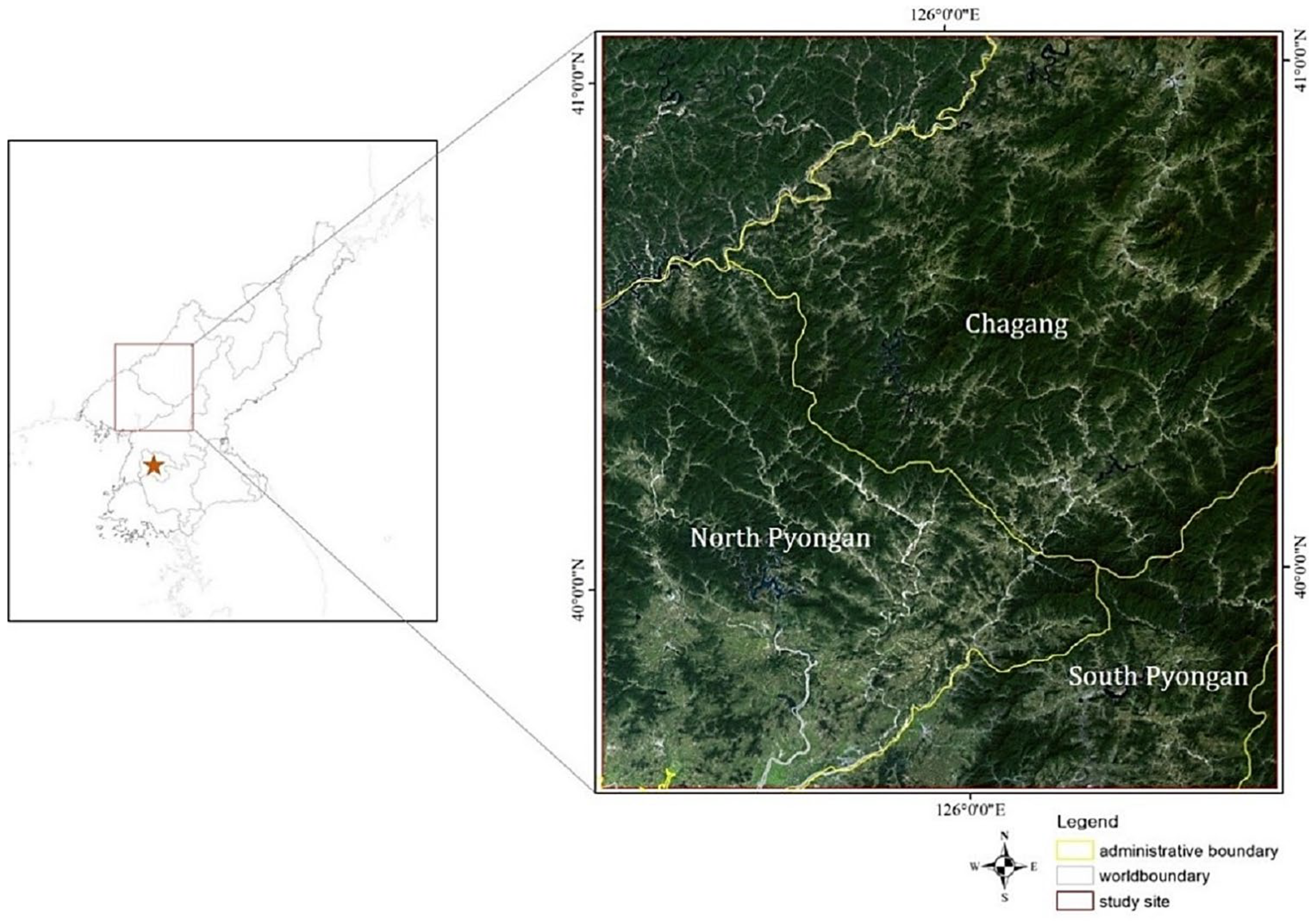
The designated experimental area for deforestation mapping corresponds to a single Landsat scene (Path/Row 117/032), as shown in Figure 1. This region encompasses parts of North Pyongan Province, South Pyongan Province, and Chagang Province in North Korea. Chagang Province is a predominantly mountainous region, with forest coverage exceeding 98%. North Pyongan borders China to the north, Chagang to the east, and South Pyongan to the south. Both North and South Pyongan Provinces have experienced substantial forest fragmentation, largely driven by deforestation and intensive agricultural expansion. Proximity to the Pyeongyang metropolitan area has further increased deforestation pressure due to heightened demands for land and resources. The two primary types of deforestation observed in this area are hillside fields and unstocked forests.

In North Korea, deforested land is often characterized by areas where trees have been logged to allow for the cultivation of crops. These activities typically shift cultivation onto steep slopes (>16°), forming terrace fields to meet subsistence needs for food and fuel. Hillside fields refer to cultivated agricultural land on sloping terrain, while unstocked forests are areas where the forest canopy cover has been reduced to below 20%, primarily due to practices such as slash-and-burn agriculture. Additionally, the study area includes plateau regions, further increasing the complexity of accurately classifying deforestation types due to the diversity of topographies and vegetation structures. These landscape variations pose significant challenges for remote sensing-based classification and emphasize the need for robust, high-resolution mapping approaches.

The satellite imagery used in this study was acquired in 2014, during a period of severe drought. This extreme climatic event led to marked vegetation degradation, exacerbating forest loss and land degradation and further highlighting the necessity for effective monitoring of deforestation and environmental stress in the region.

2.2. Key Variables for Deforestation Classification

To identify the key variables for deforestation classification—particularly for distinguishing slope farmland and non-forest areas from forestland—we adopted a systematic, multi-source approach. Reference point data for each land cover class were initially collected using Google Earth, which allowed for the interpretation of visual characteristics that are often difficult to differentiate in satellite imagery. For other land cover types, including forests, built-up areas, paddy farmland, and water bodies, we applied the visual interpretation criteria established by Jin et al. [10].

To capture the temporal dynamics of land surface changes, we derived multi-temporal variables from the MCD43A4 product at a 480 m spatial resolution (https://ladsweb.modaps.eosdis.nasa.gov/ (accessed on 16 September 2017)) from March to October, taking advantage of its high temporal frequency (

Table 1. Information on fused images.

Data Type	Acquisition Time	Spatial Resolution	Cloud	Location	Band	Role
Landsat 8 OLI	10 September 2014	30 m	0%	Path/Row 117/032	Band 3–6	Input/fine image at t1
	21 May 2014		50%			Accuracy test
	28 October 2014		100%
MCD43A4	2014 DOY253	480 m	-	H27V04	Band 1,2,6,7	Input/coarse image at t1
	2014DOY65-305		-			Input/coarse image at t2

). The daily MCD43A4 data for each month were processed using the Maximum Value Composite (MVC) method to generate monthly datasets. Then we used a set of normalized indices, including the Normalized Difference Vegetation Index (NDVI), Normalized Difference Soil Index (NDSI), and Normalized Difference Water Index (NDWI), which reflect the presence of growth of vegetation, bare soil, and surface water, respectively. These indices significantly improved classification performance compared to raw spectral reflectance data, as normalization reduces the effects of illumination variability, terrain slope, and sensor viewing angle [22]. Additionally, their sensitivity to phenological changes allows for effective monitoring of seasonal land cover transitions, from early spring greening to late-season senescence [23,24].

To further refine the variable selection process, the Random Forest (RF) algorithm was employed. RF not only provides robust classification but also evaluates the relative importance of each input variable. Based on the resulting importance rankings, we identified and selected the most influential variables to construct an optimal feature set for deforestation classification.

2.3. Spatiotemporal Data Fusion

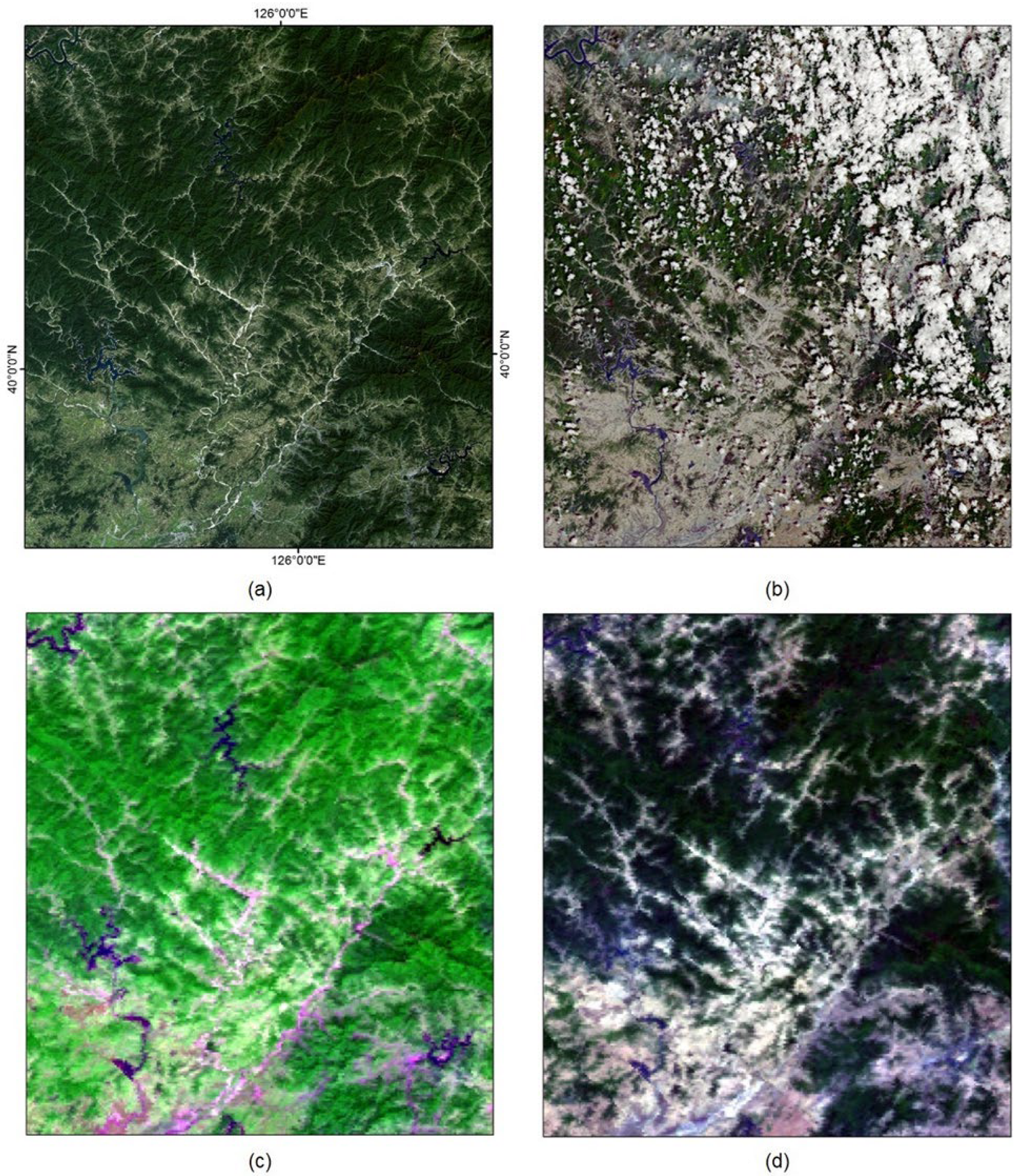
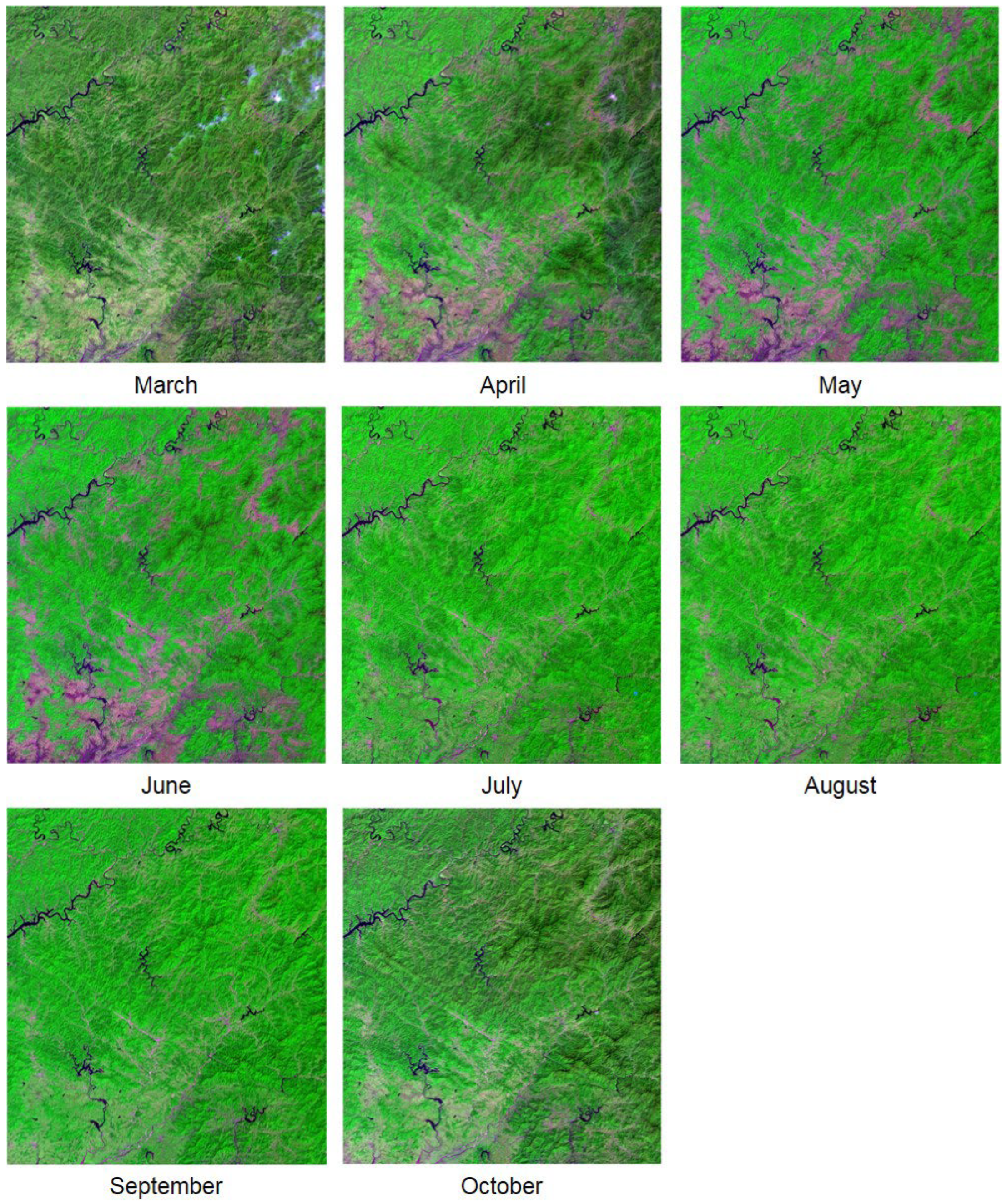
In this study, we employed the Flexible Spatiotemporal Data Fusion Algorithm (FSDAF) [25] to generate time-series images resembling Landsat-like surface reflectance. Specifically, cloud-free Landsat 8 OLI images (bands 3–6) covering a 148 km × 165 km area in southern North Korea were used as the high-resolution reference images at time point t₁. Figure 2 presents false-color composites of the Landsat and corresponding MODIS images. Two Landsat scenes (Path/Row: 117/032), acquired on 10 September 2014 (Figure 2a) and 21 May 2014 (Figure 2b), were used in the fusion analysis. The FSDAF model employed in this study incorporates several critical parameters to achieve accurate temporal data fusion. The spatial window size was set to 20, balancing the need to capture sufficient local spatial features while maintaining computational efficiency. Additionally, the scale factor was set to 16, corresponding to the ratio of coarse to fine spatial resolutions, thereby ensuring precise alignment between MODIS and Landsat imagery. These core parameters were carefully selected to optimize the performance of the FSDAF model in detecting land cover changes in the study area.

The dominant land cover types within the study area include paddy fields, flat and hillside fields, unstocked forests, plateau vegetation, and forestlands. Paddy fields and flat croplands are typically irrigated between April and June. For model training, we used the image pair from 10 September 2014 (MODIS) and 21 May 2014 (Landsat) to predict a synthetic Landsat image corresponding to Figure 2b. All Landsat images were pre-processed via atmospheric correction and subsequently converted to surface reflectance using the FLAASH module in ENVI 5.4. Details of the datasets used in the fusion process are summarized in Table 1.

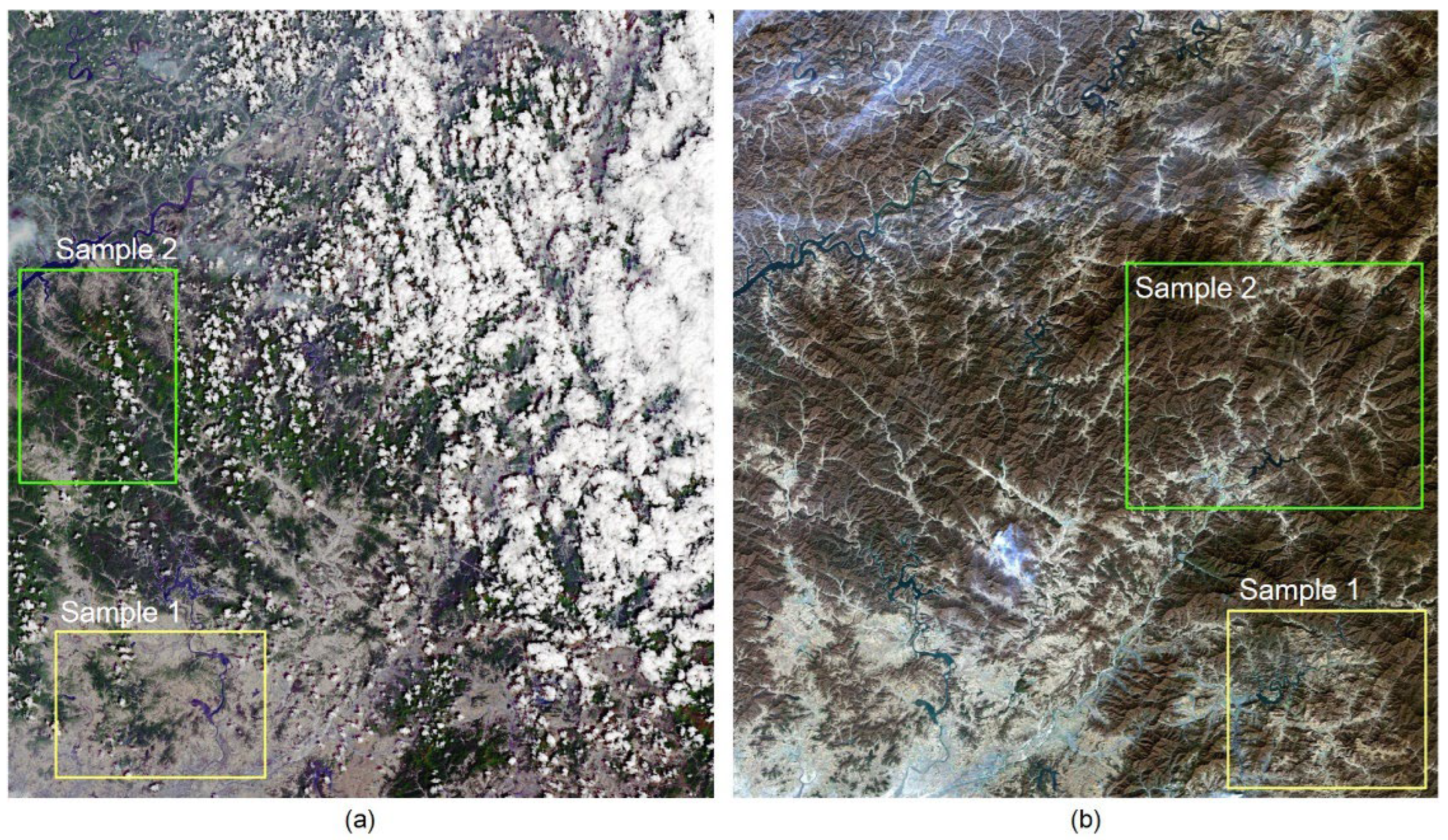
To evaluate the performance of the fusion approach, we selected two Landsat scenes acquired on 21 May 2014 and 28 October 2014, respectively. These images were intentionally chosen to represent different temporal intervals and seasonal dynamics. In addition, two representative sample sites—shown in Figure 3—were used to assess fusion accuracy under varying landscape conditions. Sample Site 1 represents a fragmented and heterogeneous environment comprising rice paddies, crop fields, water bodies, and scattered forests. In contrast, Sample Site 2 represents a relatively homogeneous landscape dominated by continuous forest and farmland. The sample sites were carefully selected to minimize the influence of cloud contamination. The accuracy of the fused imagery was evaluated both at the sample site and across the entire study area using several metrics, including the correlation coefficient (R), root mean square error (RMSE), absolute difference (AD), and structural similarity index measure (SSIM) (Equations (1)–(4)).

$$R={\displaystyle \frac{\sum (X_i-\overline{X}\left)\right(Y_i-\overline{Y})}{\sqrt{\sum {(X_i-\overline{X})}^2\sum {(Y_i-\overline{Y})}^2}}}$$

(1)

$$RMSE=\sqrt{{\displaystyle \frac{1}{n}}\sum _{i=1}^n({X_i-Y_i)}^2}$$

(2)

$$AD=\sum _{i=1}^n\left|X_i-Y_i\right|$$

(3)

where $X_i$ and $Y_i$ are the individual data points of the observed and predicted values, respectively; $\overline{X}$ and $\overline{Y}$ are means of the observed and predicted values; and $n$ is the total number of data points.

$$\mathit{S}\mathit{S}\mathit{I}\mathit{M}\left(\mathit{X},\mathit{Y}\right)={\displaystyle \frac{(\mathbf{2}{\mathit{\mu }}_{\mathit{X}}{\mathit{\mu }}_{\mathit{Y}}+{\mathit{C}}_{\mathbf{1}})(\mathbf{2}{\mathit{\sigma }}_{\mathit{X}\mathit{Y}}+{\mathit{C}}_{\mathbf{2}})}{({\mathit{\mu }}_{\mathit{X}}^{\mathbf{2}}+{\mathit{\mu }}_{\mathit{Y}}^{\mathbf{2}}+{\mathit{C}}_{\mathbf{1}})({\mathit{\sigma }}_{\mathit{X}}^{\mathbf{2}}+{\mathit{\sigma }}_{\mathit{Y}}^{\mathbf{2}}+{\mathit{C}}_{\mathbf{2}})}}$$

(4)

where ${\mathit{\mu }}_{\mathit{X}}$ and ${\mathit{\mu }}_{\mathit{Y}}$ are mean values of the images $\mathit{X}$ and $\mathit{Y}$, ${\mathit{\sigma }}_{\mathit{X}}^{\mathbf{2}}$ and ${\mathit{\sigma }}_{\mathit{Y}}^{\mathbf{2}}$ are the variances of $\mathit{X}$ and $\mathit{Y}$, ${\mathit{\sigma }}_{\mathit{X}\mathit{Y}}$ is the covariance between $\mathit{X}$ and $\mathit{Y}$, and ${\mathit{C}}_{\mathbf{1}}$ and ${\mathit{C}}_{\mathbf{2}}$ are small constants to avoid division by zero.

2.4. Classification and Validation

Following the validation of the fused datasets, we integrated the key variable ranking results with the fine-resolution fused imagery. This allowed us to extract a refined set of spatiotemporal variables at higher spatial detail, which served as the input feature set for deforestation classification. These selected variables, derived from the fused images, provided a more comprehensive representation of land surface dynamics and formed the basis for subsequent classification modeling.

In this study, we used the Random Forest (RF) algorithm to classify deforested regions. RF is an ensemble machine learning method that builds multiple decision trees, each trained on a bootstrapped subset of the data with random feature selection, which helps reduce overfitting and enhances generalization [26,27]. This approach is highly effective for high-dimensional remote sensing data and well-suited for multi-temporal imagery, as it captures seasonal and phenological variations in land cover and addresses the spectral heterogeneity that challenges traditional methods like Maximum Likelihood Classification (MLC) [28]. In our implementation, the number of trees in the RF classifier was set to 500, and the classification was repeated for 200 runs to ensure stability and robustness of the results. Although recent advances in artificial intelligence—such as deep learning models like U-Net or artificial neural networks (ANNs)—have demonstrated excellent performance in land cover classification tasks, these approaches generally require large-scale, well-annotated training datasets and significant computational resources. Given the limited availability of high-quality labeled data and restricted data access in the study area, the application of deep learning models such as U-Net or ANN was not considered feasible for this research.

Ground truth points for accuracy assessment were identified using Google Earth imagery, applying the same visual criteria as those used for the training data to determine land cover types. Approximately 50–60 points were selected for each land cover class to serve as test samples. The classification results were then extracted for these points to construct the test dataset that was used for accuracy evaluation. To assess the classification performance, a confusion matrix was employed to calculate overall accuracy, user’s accuracy, and producer’s accuracy for each land cover class. In addition, the Kappa coefficient was computed to quantify the level of agreement between the classification results and the reference (ground truth) data [29].

3. Results

3.1. Key Variables for Deforestation Classification

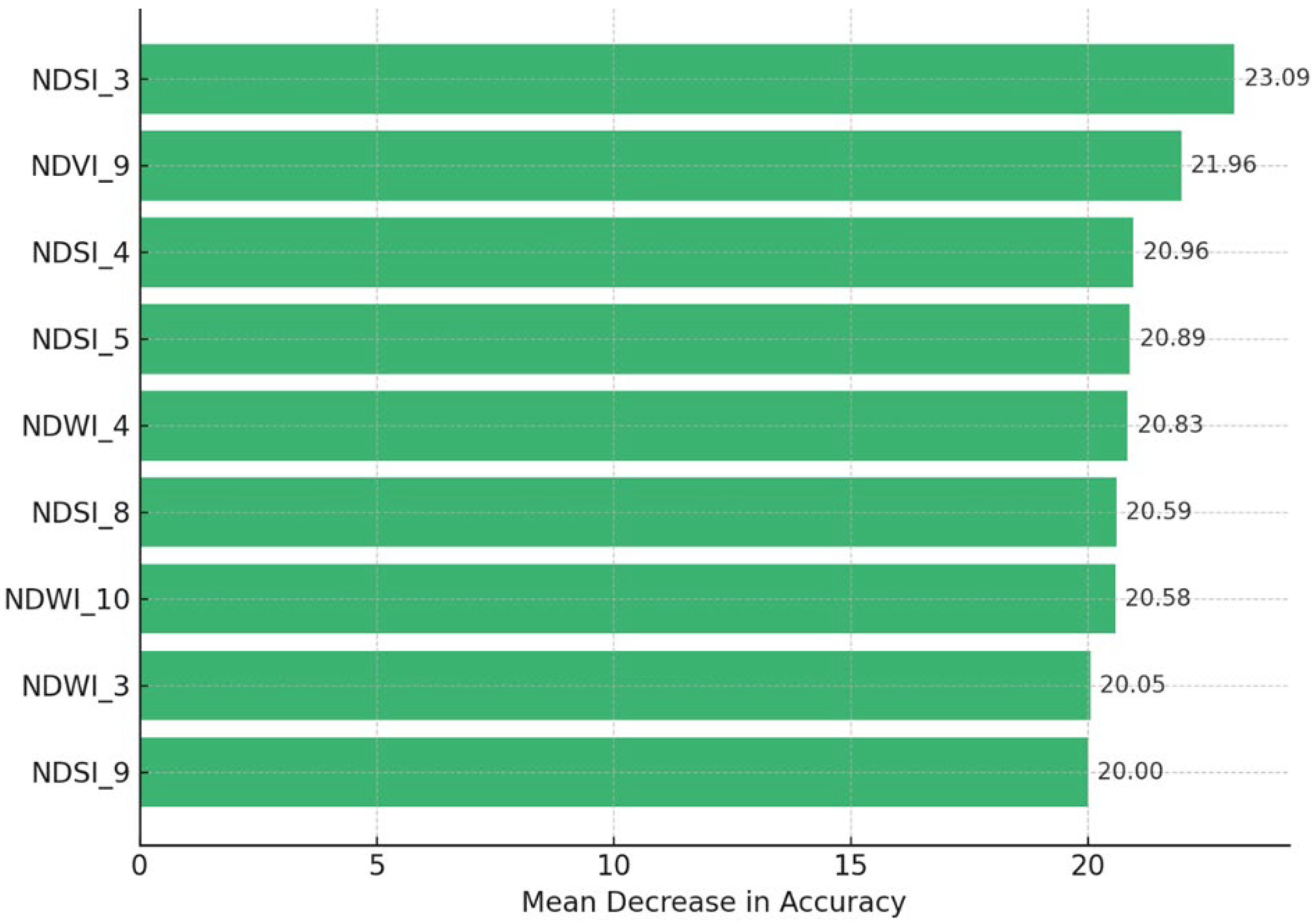
To determine the most influential variables for deforestation classification, especially for distinguishing slope farmlands and non-forest areas, we employed the Random Forest (RF) algorithm. The variable importance was quantified using the Mean Decrease Accuracy (MDA) metric, which evaluates the contribution of each variable to the model’s predictive performance. Higher MDA values indicate greater relevance for classification tasks. The results (Figure 4) reveal that the top-ranked variable was NDSI_3 (the NDSI for March), followed closely by NDVI_9 (the NDVI for September) and NDSI_4. These variables exhibited the highest MDA values, suggesting their strong ability to capture phenological and seasonal dynamics, which is critical for identifying deforestation patterns.

Among the nine most important variables (which MDA scores are over 20), the majority were derived from the NDSI and NDVI, indicating that vegetation greenness and seasonal snow cover changes play pivotal roles in distinguishing deforested areas from intact forest or other land cover types. Variables such as NDWI_4, NDWI_10, and NDWI_3 also appeared among the top contributors, highlighting the complementary importance of surface moisture and hydrological conditions, particularly in differentiating between forest, waterlogged land, and recently disturbed areas. Conversely, variables such as NDWI_7, NDWI_9, and NDWI_5 had the lowest MDA scores, implying relatively weaker contributions during these periods. This might be attributed to lower phenological contrast or less distinctive moisture dynamics at those time steps.

Overall, the use of multi-temporal indices allowed the model to capture seasonal vegetation and environmental dynamics, enhancing the discrimination of deforested landscapes. The integration of NDSI, NDVI, and NDWI from different phenological phases provides a robust basis for the classification of complex land cover transitions in heterogeneous environments.

3.2. Key Variables in a Fine Resolution

The blended images generated by the FSDAF method are presented in Figure 5 and Figure 6, offering a visual comparison with reference imagery. These figures clearly illustrate that the fusion algorithm effectively preserves both spatial detail and seasonal phenological characteristics. This observation is further supported by a quantitative evaluation using two original Landsat images acquired on 21 May and 28 October 2014. The accuracy metrics are summarized in

Table 2. Accuracy assessment of spatiotemporal data fusion method applied to pixels at all points, Sample Site 1 and Sample Site 2. Sample Site 1 covers heterogeneous areas, but the main land cover is farmland; Sample Site 2 covers homogeneous areas, where the main land cover is forest.

Date		29 May 2014				28 October 2014
Indicator		R	RMSE	AD	SSIM	R	RMSE	AD	SSIM
All	Red	0.880	0.027	0.003	0.834	0.818	0.028	0.011	0.899
	NIR	0.850	0.061	0.005	0.853	0.826	0.063	−0.044	0.828
	SWIR1	0.855	0.037	0.005	0.875	0.878	0.058	0.024	0.841
	SWIR2	0.813	0.036	0.002	0.824	0.824	0.055	0.030	0.870
Sample Site 1	Red	0.726	0.0469	0.009	0.809	0.721	0.029	0.009	0.868
	NIR	0.703	0.0109	0.006	0.846	0.708	0.065	−0.040	0.902
	SWIR1	0.809	0.064	0.020	0.869	0.785	0.060	0.019	0.769
	SWIR2	0.742	0.061	0.006	0.889	0.740	0.053	0.023	0.840
Sample Site 2	Red	0.847	0.026	−0.002	0.824	0.830	0.027	0.004	0.979
	NIR	0.905	0.063	0.004	0.887	0.825	0.072	−0.05	0.896
	SWIR1	0.936	0.030	0.002	0.897	0.891	0.066	0.018	0.949
	SWIR2	0.869	0.035	0.001	0.821	0.874	0.052	0.021	0.977

.

The fused images successfully incorporate temporal variation into the input Landsat data, resulting in high correlation coefficients (R > 0.8) and structural similarity index (SSIM) values approaching 0.9, indicating a strong resemblance to actual Landsat observations. However, in Sample Site 1—characterized by high land cover heterogeneity and pronounced spectral variation—lower correlation values, particularly in the NIR band, were observed. In contrast, Sample Site 2, which predominantly consists of homogeneous forest cover, yielded an R value close to 0.9, demonstrating strong agreement between the atmospherically corrected Landsat images and the fused results. Additionally, the RMSE, absolute difference (AD), and SSIM values confirm the high predictive accuracy in homogeneous landscapes.

This study employed two Landsat images, acquired in different seasons and at varying temporal intervals. The base image used for fusion was captured in September, while the target images were from May and October. Despite the temporal gaps, all evaluation metrics indicate consistently high accuracy across the scenes. These results suggest that the fusion performance of FSDAF is more sensitive to spatial heterogeneity than to temporal separation between image acquisitions. The fused spectral bands were subsequently used to derive the key variables for fine-resolution deforestation classification.

3.3. Classification Results

The classification results demonstrated robust performance, achieving an overall accuracy of 86.1% and a kappa coefficient of 0.837, indicating strong agreement between the classification outputs and the reference data (

Table 3. Confusion matrix for land cover classification of the study area during 2014.

	Reference Data	Plateau Vegetation	Forest	Unstocked Forest	Hillside Field	Paddy	Field	Water	Total	Producer’s
Map Results
Plateau vegetation		44	0	0	0	0	0	0	44	100%
Forest		3	67	4	0	5	0	0	79	84.8%
Unstocked forest		0	0	42	1	0	0	0	43	97.7%
Hillside field		0	0	7	49	2	0	0	58	84.5%
Paddy		0	0	4	6	34	0	0	44	77.3%
Field		1	0	2	4	10	52	3	72	72.2%
Water		0	0	0	0	0	3	50	53	94.3%
Total		48	67	59	60	51	55	53	393
User’s		91.7%	100%	71.2%	81.7%	66.7%	94.5%	94.5%	94.3%
Overall accuracy: 0.861 Kappa: 0.837

). Most land cover types, such as plateau vegetation, forest, water, and unstocked forest, exhibited high producer’s and user’s accuracies. Plateau vegetation was identified with a producer’s accuracy of 100% and a user’s accuracy of 91.7%, indicating minimal confusion with other classes. Forest showed good reliability, with a producer’s accuracy of 84.8% and a user’s accuracy of 100%, suggesting accurate identification with minimal commission errors. Water also showed excellent classification accuracy, with a producer’s accuracy of 94.3% and a user’s accuracy of 94.3%, indicating strong consistency between mapped results and reference data.

However, some categories displayed relatively lower classification precision. Paddy fields had the lowest user’s accuracy (66.7%), indicating significant misclassification with other land cover types such as fields and hillside fields, likely due to spectral similarities and overlapping phenological characteristics. Field classes exhibited a moderate producer’s accuracy of 72.2%, reflecting notable omission errors, while the user’s accuracy was higher at 94.5%, suggesting fewer commission errors. Unstocked forests achieved a high producer’s accuracy of 97.7%, demonstrating effective detection, but had a lower user’s accuracy of 71.2%, indicating considerable commission errors where pixels classified as unstocked forests frequently belonged to hillside fields or fields. Hillside fields presented moderate accuracies, with a producer’s accuracy of 84.5% and user’s accuracy of 81.7%, suggesting balanced occurrence of both omission and commission errors. This indicates a challenge in distinguishing hillside fields from spectrally similar classes, particularly unstocked forests and fields.

The confusion matrix (Table 3) further illustrates specific misclassification patterns. Notably, hillside fields and paddy fields showed confusion with unstocked forests and fields, reflecting the phenological and spectral similarities among these land cover categories. Future classification improvements could benefit from integrating additional temporal or spectral indices and using advanced classification algorithms to better differentiate spectrally similar land cover classes.

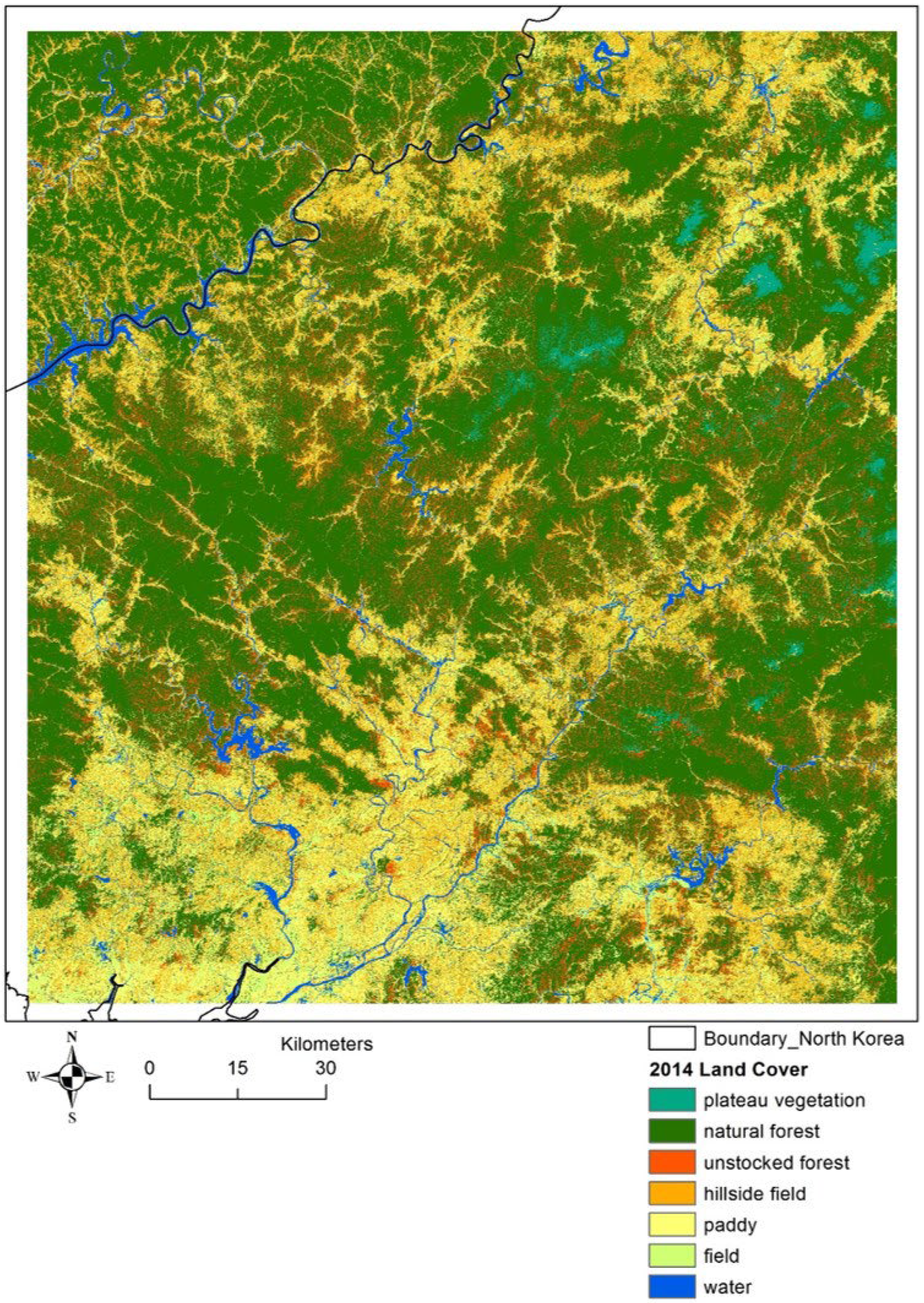
Based on the land cover classification map (Figure 7), distinct spatial patterns of deforested areas, particularly unstocked forests and hillside fields, can be observed within the study area. These deforested zones predominantly appear as fragmented patches dispersed around the margins or within proximity to intact forested regions, signifying potential areas of human-induced disturbance or natural degradation. Specifically, hillside fields exhibit widespread distribution across slopes, while unstocked forests tend to occur more irregularly and patchily, suggesting varying degrees and histories of deforestation.

Interestingly, plateau vegetation exhibits spatial and spectral characteristics that are remarkably similar to deforested areas, posing a significant challenge in classification. However, differences in snowmelt timing between plateau vegetation and deforested areas provided critical phenological signals that were effectively captured by the extracted temporal variables. This phenology-driven differentiation notably enhanced the classification accuracy, facilitating clear distinctions between plateau vegetation and deforested categories, despite their inherent spectral similarities.

The successful utilization of variables underscores the value of incorporating phenological information into land cover classification workflows, significantly improving the reliability of identifying and monitoring deforested landscapes.

4. Discussion

In this study, we leveraged phenology-based indices derived from fused satellite time-series to map land cover types, taking into account vegetation growth patterns, soil exposure, and vegetation moisture status. This comprehensive approach enabled the accurate identification of forested areas characterized by healthy vegetation, high canopy cover, and sufficient moisture, while also capturing deforested areas—namely unstocked forests and hillside fields—with improved precision compared to traditional NDVI-based methods.

Despite these improvements, certain misclassifications persist, primarily due to the intrinsic challenges of differentiating spectrally similar land cover types in heterogeneous landscapes. As shown in Table 3, unstocked forests and hillside fields, which represent the principal deforested categories in the study area, often share overlapping spectral and phenological characteristics. This overlap is exacerbated by seasonal variation, mixed land use, and the transitional nature of vegetation cover. Additionally, topographic factors such as slope and shadowing can further confound spectral signals, reducing class separability and leading to commission and omission errors. In particular, hillside fields exhibited higher omission errors, as true hillside areas were sometimes misclassified as fields or unstocked forests due to their fragmented and patchy distribution. Conversely, unstocked forests suffered from higher commission errors, being frequently confused with hillside fields.

A noteworthy finding is that plateau vegetation and deforested areas (unstocked forest, hillside field) display similar spatial and spectral patterns, making them difficult to distinguish using conventional indices. However, by integrating phenology-driven variables—specifically differences in snowmelt timing—our approach successfully exploited the phenological distinctions between these classes. The snowmelt process occurs earlier in deforested areas than plateau vegetation, providing an additional temporal signal that enhances classification accuracy. This demonstrates the value of including temporal ecological information for resolving ambiguities between spectrally similar land cover types, a strategy that has also been highlighted in recent studies on phenology-based land cover mapping [10,14].

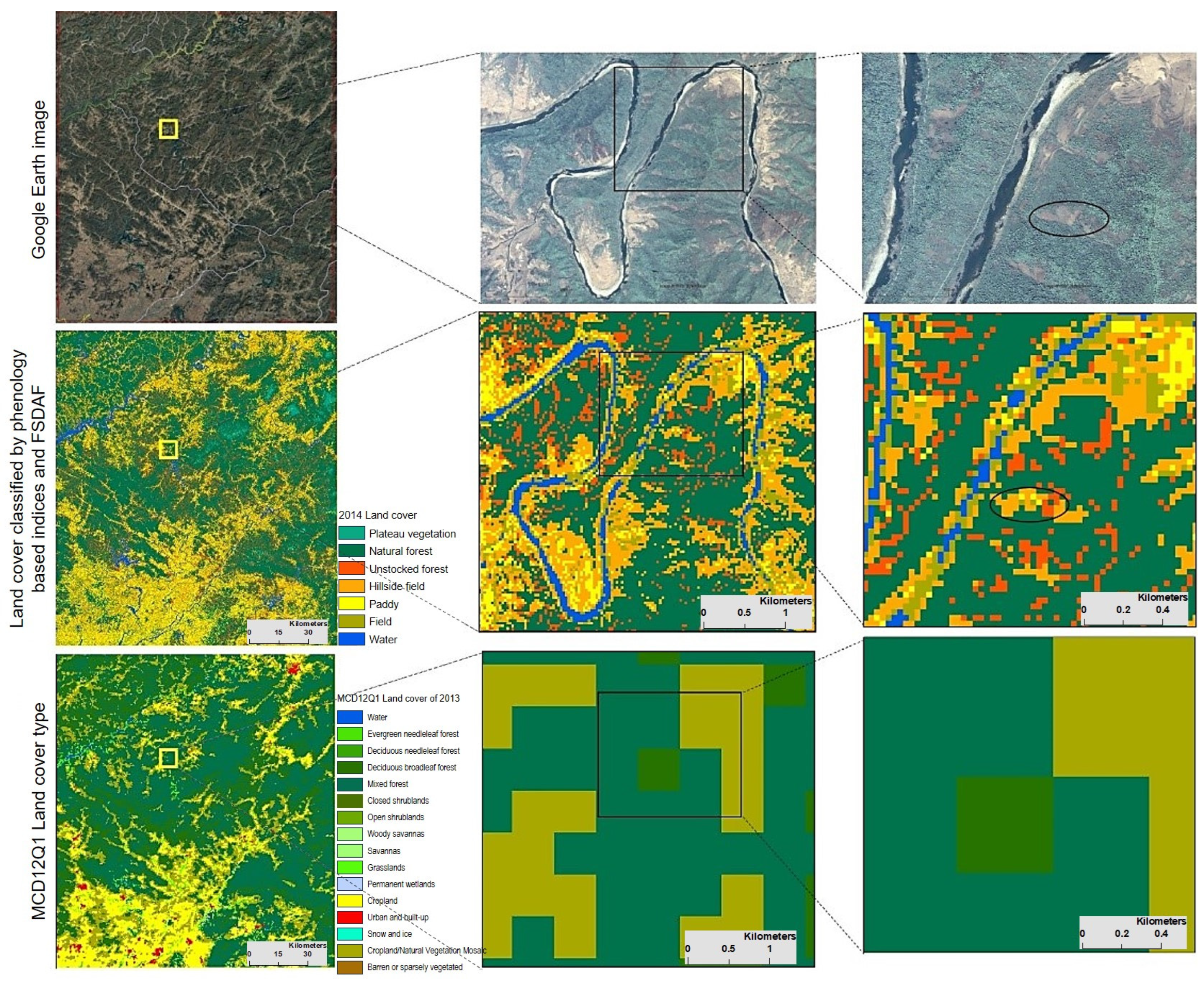
Our method’s advantages are further underscored by comparison with both the MCD12Q1 land cover product and high-resolution Google Earth imagery (Figure 8). As illustrated in Figure 8, the MCD12Q1 dataset, which is based on global-scale classification and 500 m spatial resolution, failed to accurately reflect the detailed deforestation and land cover heterogeneity observed in North Korea. Its generalized categories, such as mixed forest, deciduous broadleaf forest, and cropland, are insufficient for regional ecological assessments, missing the patchy and fragmented distributions that are typical of deforested zones. In contrast, our classification not only distinguished a broader spectrum of land cover types but also provided more spatially realistic and ecologically relevant results. This improvement is attributed to the integration of high-frequency temporal data and the use of region-specific phenological indices, consistent with recent trends in remote sensing research that advocate for multi-source, temporally rich data fusion to improve local land cover classification [15,16].

Nevertheless, challenges remain. The limited availability of labeled samples and restricted access to ground truth data in North Korea pose significant constraints for training advanced deep learning models, such as U-Net or Transformer-based architectures, which have shown promise in other deforestation studies [17]. Future research will aim to address these limitations by expanding ground reference data collection and exploring the application of cutting-edge deep learning methods as more annotated datasets become available.

In summary, while our phenology-informed framework demonstrates superior mapping accuracy and spatial detail compared to widely used global products, continued methodological refinement and expanded field validation are essential for further improving the reliability of regional deforestation and land degradation assessments.

5. Conclusions

This study presents a novel and cost-effective approach for mapping deforestation, with a particular focus on distinguishing hillside fields and unstocked forest areas within heterogeneous vegetation landscapes. By integrating spatiotemporal data fusion and multi-temporal indices, the proposed method significantly enhances classification accuracy and provides reliable identification of deforested areas. This is especially valuable for monitoring vegetation dynamics in ecologically sensitive and data-limited regions such as North Korea.

Although the satellite data used in this study corresponds to the year 2014—due to the availability of ground truth data from the same period—the primary objective was to demonstrate the applicability and effectiveness of a new classification framework that improves both the spatial and temporal resolution of deforestation type mapping. Importantly, while this study uses a single-year dataset as a proof-of-concept, the FSDAF framework itself is inherently scalable and can be readily extended for long-term monitoring and multi-year time-series analysis. When combined with additional multi-temporal datasets, such as high-frequency Sentinel-2 imagery, this approach can support continuous or near-real-time monitoring of land cover change. Clarifying this capacity for temporal extension further underscores the broader utility and potential of the methodology for deforestation monitoring at regional and national scales. Future work should focus on expanding both the temporal scope of analysis and the field-based reference data to fully realize the benefits of ongoing monitoring and real-time forest tracking.

The methodological contribution of this study lies in its potential adaptability to other regions facing similar classification challenges. The mapping and monitoring framework developed here has broader applicability beyond forest degradation, with potential utility in supporting multi-objective forest landscape restoration (FLR), including agricultural planning, biodiversity conservation, and climate change adaptation. Accurate identification of deforestation and degradation areas provides essential baseline data for prioritizing reforestation and management interventions.

Furthermore, establishing a continuous forest inventory system that reflects regional characteristics—such as the persistent degradation patterns and shifting land use in North Korea—is of critical importance. By enabling precise monitoring and evidence-based decision-making, this study contributes to the broader goal of sustainable forest management and ecological resilience. The proposed approach can support policymakers, conservation agencies, and land managers in their efforts to restore and sustainably utilize forest resources in North Korea and other similar environments worldwide.