Abstract
Under intensified global climate change and complex land use transitions, the Leaf Area Index (LAI) serves as a key ecological indicator to monitor vegetation responses to natural and anthropogenic factors. This study provided a comprehensive spatiotemporal diagnosis of the LAI and uniquely integrated remote sensing data with the Geodetector model to quantitatively assess both individual and interactive effects of natural and human drivers. Specifically, we analyzed LAI dynamics in the Jinsha River Basin from 2000 to 2023 using Sen’s Slope and Mann–Kendall tests, combined with Geodetector modeling to identify drivers and their interactions. Furthermore, ARIMA-based forecasting offered forward-looking insights to support land use planning and ecosystem resilience. Results revealed a fluctuating upward trend in LAI, with larger areas improving than degrading, and distinct seasonal and spatial patterns, with a notably higher LAI in southern regions. Elevation and temperature were the primary drivers, explaining 57% and 54% of spatial variation, respectively, with their combined effects further enhancing explanatory power. The future LAI trend appeared stable without significant changes. These findings demonstrated LAI’s utility for assessing land use change impacts and ecological sustainability, providing a scientific basis for land use optimization, ecological restoration, and sustainable regional development under the human–earth system framework.
1. Introduction
Over the past few decades, global climate change and escalating ecological deterioration have significantly impacted the structure, functions, and services of ecosystems. Rising temperatures, changing precipitation patterns, and increasing human activity have led to vegetation degradation, biodiversity loss, and desertification all over the world [1,2]. In this context, understanding how vegetation evolves in response to both natural and anthropogenic influences is essential for monitoring ecological shifts and promoting long-term ecosystem sustainability [3]. In particular, land use and cover change (LUCC), as a key anthropogenic driver, has notably altered vegetation patterns and ecosystem processes, emphasizing the need for long-term, accurate monitoring of vegetation changes.
The Leaf Area Index (LAI) is ecologically significant and serves as a core indicator for measuring the canopy structure of vegetation and the productivity of the ecosystem. The LAI is typically defined as half the ratio of total leaf surface area to the corresponding ground area. In most studies, the unit is directly marked as m2/m2 or stated as dimensionless. It reflects vegetation growth conditions and functional traits, and it is a vital proxy for vegetation greenness, energy exchange, and biogeochemical processes [4]. The LAI plays a critical role in estimating crop yields, monitoring vegetation phenology, simulating land–atmosphere fluxes, and assessing photosynthetic potential and water use efficiency [5,6,7,8,9]. Due to its sensitivity to land use conversion, degradation, and restoration, analyzing the spatiotemporal patterns and drivers of the LAI has both theoretical and practical significance for understanding ecosystem functions and improving ecological management [2].
Among various vegetation indicators such as the Normalized Difference Vegetation Index (NDVI), the Enhanced Vegetation Index (EVI), and Fraction Vegetation Coverage (FVC), this study focused on the LAI due to its superior ecological interpretability. Unlike spectral indices that primarily reflect vegetation greenness, the LAI directly quantifies canopy structure and physiological traits, including photosynthesis and transpiration. As a key input for ecosystem models, the LAI is indispensable in simulating carbon cycles, material flows, and energy balance [10,11]. These attributes make the LAI more suitable for long-term ecological monitoring and environmental assessment.
The research results based on the LAI can not only reflect the growth status of vegetation but also deeply reveal its productivity and carbon sink capacity. Compared with studies that solely rely on spectral vegetation indices, they can provide more comprehensive information on ecological processes. In addition, the LAI data provided by satellite remote sensing products, such as the Moderate Resolution Imaging Spectroradiometer (MODIS), have the advantages of strong continuity, high data quality, and global-scale standardization, making spatio-temporal analysis more scientific and comparable. In complex terrains like the Jinsha River Basin, where human activities are frequent, the LAI provides a more reliable indicator for assessing the combined impacts of climate, topography, and anthropogenic pressures on vegetation structure and function.
Existing studies have explored the evolution characteristics of the LAI and its relationship with driving factors, such as climatic variations and anthropogenic activities at the global and regional scales. Piao et al. (2015) [12] analyzed vegetation greening trends in China over the past three decades using three remote sensing LAI datasets, including the Global Inventory Modeling and Mapping Studies (GIMMS) LAI and the Global Land Surface Satellite (GLASS) LAI. The results showed that the global long-term satellite LAI had improved significantly since 1982, and the values of remote sensing products had exhibited a generally upward trend across the majority of regions. China’s greening rate surpassed the global average by approximately 24%. Under future climate change scenarios, it was expected that the global average LAI would continue to increase. However, there are obvious differences among the changes in the regional LAI [13]. At the regional-scale, Sun et al. (2021) [14] investigated the correlations between the LAI and climatic variables in ecologically fragile regions of China and confirmed that temperature was the dominant meteorological factor affecting the LAI. Zhang et al. (2002) [15] studied the response mechanism of the vegetation LAI to temperature and precipitation at global scale. Furthermore, the changes in the long-term LAI can reveal the evolution process of regional ecosystems and have high application value in monitoring the growth status of vegetation and estimating the yield of agricultural products. Specifically in typical areas, Yao et al. (2024) [16] analyzed the spatiotemporal variations in the LAI in Hainan Island and believed that the promotion of vegetation growth by rising temperatures exhibited a saturation effect. Zou et al. (2022) [17] examined the spatiotemporal vegetation dynamics of the Beijing–Tianjin–Hebei region from 2001 to 2020, demonstrating that the LAI increased in tandem with rising temperature and precipitation. Reygadas et al. (2020) [18] evaluated the relationship between the intra-annual and seasonal LAI and surface temperature in the central region of Mexico from 2002 to 2017. Liang et al. (2015) [19] examined vegetation dynamics in Xinjiang over the period 1982 to 2012 using the GLASS LAI dataset, providing strong support for the detection of ecological changes in arid areas. Overall, the research on the LAI has been relatively rich and systematic. The related theoretical and methodological system has become increasingly mature, laying a solid foundation for a comprehensive understanding of vegetation dynamics and its driving mechanisms.
Long-term series of vegetation parameters can reflect regional ecological evolution, offering insights into both the quantity and quality of vegetation change. Common methods to detect long-term trends include the coefficient of variation (CV), slope, standardized anomalies, Mann–Kendall (M-K) test, Sen’s Slope, and Empirical Orthogonal Function (EOF) analysis. While the CV assesses ecosystem stability and disturbances, it lacks trend direction. Slope indicates the rate and direction of change but struggles with nonlinear patterns. Standardized anomalies detect abnormal values but not trends. The M-K test and Sen’s Slope provide non-parametric tools for trend analysis without assuming normality [20], although they cannot identify non-monotonic trends. EOF analysis is effective for large-scale variability but not suitable for nonlinear transitions [21]. Based on these considerations, this study adopts Sen’s Slope and the M-K test to assess long-term LAI changes due to their robustness and compatibility with long-term remote sensing data.
While many studies have applied linear correlation methods to explore the relationship between LAI and various natural and socio-economic factors, these approaches are limited in quantifying the relative influence of each factor and cannot effectively reveal interactions among multiple drivers [22,23,24]. To overcome these deficiencies, the Geodetector, as a method for analyzing spatial heterogeneity and its driving factors, has been widely used in the fields of ecology and environment in recent years. This method can not only identify the dominant factors influencing the changes in the LAI but also quantitatively evaluate the explanatory power of each factor for the changes in the LAI under independent and interaction effects, and it has strong interpretability and adaptability [25]. Therefore, the Geodetector model has advantages to conduct the quantitative analysis of the driving mechanism of LAI changes, with the aim of revealing more comprehensively the independent and synergistic effects of multi-drivers.
At present, the research related to the LAI mainly focused on major agricultural areas, forest ecosystems at global scale or in China [26], grasslands, and ecological restoration areas, as well as on monitoring and verification on a national scale [27]. However, research on the ecosystem LAI at the watershed scale is relatively lacking. The Jinsha River Basin, as a key component of the upper Yangtze River, undertakes the key functions of the Yangtze River Basin ecosystem, and its ecological environment has always been the focus of attention of the government and the academic community. The Jinsha River Basin occupies a uniquely distinctive geographic position, and the natural environment in each region varies significantly [28]. The complex natural conditions within the basin have given birth to abundant vegetation resources. However, at the same time, this complex ecological environment, along with increasingly frequent human activities, has significantly enhanced the ecological vulnerability and sensitivity of this region. Therefore, a comprehensive long-term assessment of the spatiotemporal evolution of the LAI in the Jinsha River Basin is essential not only to deepen the understanding of basin-wide vegetation changes but also to provide scientific insights and policy guidance to support sustainable ecosystem management.
Firstly, this study applied the Sen’s Slope method and the M-K trend analysis method to conduct a quantitative study on the long-term changing trend of the LAI in the Jinsha River Basin using MODIS LAI data from 2000 to 2023. Secondly, spatial autocorrelation analysis was applied to determine the spatial distribution patterns and trends of the LAI. Thirdly, the natural and human impact factors of the LAI were analyzed by the Geodetector model and Multiple Linear Regression (MLR). Finally, based on the future trend of the LAI, the study proposes targeted policy recommendations aimed at optimizing land use structure, enhancing ecosystem resilience, and supporting sustainable land use planning and territorial development in the Jinsha River Basin. This integrated approach provides scientific insights and methodological support for better aligning ecological monitoring with land management decisions in ecologically sensitive river basins. The specific research framework diagram is as follows (Figure 1).
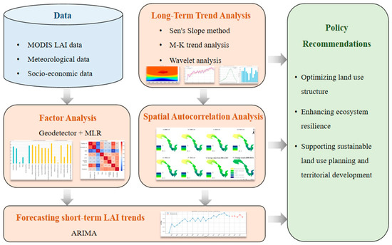
Figure 1.
Research framework of this study.
2. Materials and Methods
2.1. Research Area
The Jinsha River rises in the Qinghai–Tibet Plateau and traverses the upper reaches of the Yangtze River, spanning longitudes 90–105°E and latitudes 24–36°N (Figure 2). It flows eastward through Qinghai, Tibet, the western part of the Sichuan Plateau and the northern part of the Yunnan–Guizhou Plateau, and finally joins the Minjiang River in Yibin, southeastern Sichuan. The main stream of the Jinsha River is 3481 km long, and its drainage area is approximately 470,000 square kilometers. The Jinsha River Basin is mainly situated within the eastern part of the Qinghai–Tibet Plateau and the Hengduan Mountain region [29,30].
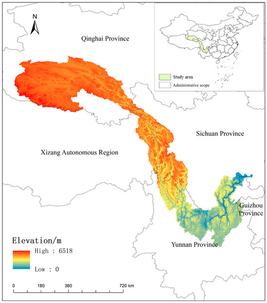
Figure 2.
Geographical location of the Jinsha River Basin, China.
The Jinsha River Basin is located in the transitional zone between the first and second tiers of China. The terrain conditions are particularly complex, with plateaus, canyons, basins, and hills crisscrossing, and high mountains and deep valleys alternating. Affected by the intense topographic undulations and a latitude span of about 10°, the climate types within the basin are diverse, showing obvious regional differentiation. From the Qinghai–Tibet Plateau, with long winters and almost no summers, to the Hengduan Mountains, with distinct four seasons, to the dry–hot river valleys, with extended summers and short winters, and to the Yunnan–Guizhou Plateau, with a mild climate throughout the year, a diverse climate zoning pattern is formed [28]. Due to variations in natural geography and socio-economic development, the population density across the Jinsha River Basin exhibits significant spatial differences, generally increasing from the northwest to the southeast [31]. In addition, the industrial types within the basin are diverse. Industrial activities such as tourism, mineral resource development and hydropower construction are widely distributed, and the characteristics of regional economic development are obvious. Therefore, taking the Jinsha River Basin as the study area, it is highly typical and demonstrates significant practical value to analyze the dynamics and interaction effects of the LAI. The Yalong River is the largest tributary of the Jinsha River, and its drainage area is approximately 136,000 square kilometers. To narrow the scope of this study, the Yalong River Basin was excluded from the study area.
2.2. Data Sources
2.2.1. MODIS LAI
To select the most appropriate LAI dataset for this study, we first compared long-term LAI trends derived from MODIS, GIMMS, and GLASS products over overlapping periods and spatial regions [5]. The results showed a general consistency in trend direction among the three datasets. However, considering the MODIS LAI’s higher temporal resolution, better spatial completeness, and continuity, we selected it as the primary data source for subsequent analyses.
The MODIS LAI products are LAI data obtained by MODIS and are widely used in agricultural, ecological, climate, and geographical science research. Based on remote sensing data from MODIS sensors, MODIS LAI data of the MOD15A2H product set was used to call, pre-process, and download through Google Earth Engine (GEE) remote sensing big data cloud platform, with a time resolution of 30 d and a spatial resolution of 250 m. After pre-processing in the GEE platform, mosaic, projection, transformation, and clipping were performed. Then, a Maximum Value Composition (MVC) method was applied to merge the monthly maximum LAI data to minimize the impact of clouds, atmospheric effects, scanning angles, and solar zenith angles on image quality.
2.2.2. Elevation and Slope
Elevation used in this study originates from the Shuttle Radar Topography Mission (SRTM) Version 4 dataset, made available by the Consultative Group for International Agricultural Research Consortium for Spatial Information (CGIAR-CSI). The dataset can be obtained from the corresponding platform, featuring a spatial resolution of 90 m, and is provided in the GeoTIFF format. The GEE platform was used to overlay, clip, download, and extract elevation, slope, and other relevant factors for analyzing their impact on vegetation coverage.
2.2.3. Meteorological Data
Climate drivers exert a decisive influence on the spatiotemporal dynamics of vegetation, as shifts in thermal and hydrological regimes critically underpin plant productivity. In this study, two principal climate indicators—annual mean 2 m air temperature, and total annual precipitation—were selected. The relevant data were obtained from the ERA5 (Fifth Generation of the ECMWF Reanalysis for the Global Climate and Weather) dataset via the Google Earth Engine (GEE) platform. Since the native resolution of the ERA5 temperature and precipitation data is 0.25°, both variables were resampled to 250 m resolution using bilinear interpolation to ensure spatial consistency with the MODIS LAI data. This interpolation does not introduce new spatial information but facilitates integrated spatial analysis across all input layers. The annual mean temperature was calculated by averaging monthly values from January to December, while the total annual precipitation was obtained by summing the respective monthly accumulations at the basin scale.
2.2.4. Human Activity Factor
For anthropogenic drivers, gridded population density datasets were employed, which were obtained from the WorldPop project (https://www.worldpop.org, accessed on 1 March 2025).
2.2.5. Land Use Type Data
Land use type has a direct impact on the growth conditions of vegetation. Therefore, there is a complex connection between land use type and the LAI. In this study, GLC-FCS30D datasets span from 1985 to 2022 at a resolution of 30 m were used and can be obtained from https://zenodo.org/records/8239305 (accessed on 1 March 2025). Based on the regional characteristics of the Jinsha River basin, this study combined the 35 categories into 13 categories. Different land cover types reflect different human land use patterns and are regarded as important factors influencing vegetation coverage. The data used in this study are listed in Table 1.

Table 1.
Data required for the study and its sources (The websites were accessed on 1 March 2025).
2.3. Methodology
2.3.1. Analysis of Vegetation Dynamics
- 1.
- The M-K test, paired with the Sen’s Slope method
The Sen’s Slope method computes the median rate of change across a long-term time series, thereby quantifying the magnitude of upward or downward trends while effectively mitigating the influence of outliers and reducing data errors. Owing to these robust characteristics, it is extensively applied in trend analyses across meteorological, hydrological, ecological, and related areas [32].
The M-K test is a widely used non-parametric method for detecting the presence and significance of trends in long-term time series data [16,33]. It not only evaluates the significance of temporal trends but can also identify abrupt changes (mutations) in the time series.
- 2.
- Wavelet analysis
Wavelet analysis is an effective method for analyzing non-stationary time series by decomposing signals into time and frequency components. In this study, the Continuous Wavelet Transform (CWT) was applied to identify the temporal variation and periodic characteristics of the LAI. The Morlet wavelet was used as the mother wavelet due to its good time-frequency localization. The wavelet power spectrum was calculated to reveal dominant cycles and their changes over time, while the global wavelet spectrum was used to identify overall periodicities. Significance testing against a red-noise background was conducted to ensure the reliability of results. This method enables a multi-scale understanding of vegetation dynamics and their temporal patterns.
- 3.
- Spatial hot spot analysis
In ArcGIS Spatial Statistics, Global Moran’s I was used to quantify spatial autocorrelation. Spatial relationships were parameterized using inverse-distance weighting scheme based on Euclidean distance as the selected metric.
Hot spot analysis is a spatial statistics technique used to detect areas within the study region that exhibit statistically significant clusters of high or low values [34]. This method is based on the spatial autocorrelation theory and usually adopts the Getis-Ord Gi* index to quantify the aggregation pattern of spatial data, so as to reveal the spatial distribution law of specific phenomena (such as environmental pollution, land use change, social and economic activities, etc.). The core idea is to evaluate whether an observation has a high or low spatial aggregation in its neighborhood. When calculating the Getis-Ord Gi* index, the attribute values of the research unit and their spatial adjacency weights are taken into account to check whether the unit is located in a significant region of high value (hot spot) or low value (cold spot). The formula is as follows:
where represents the Getis-Ord statistic for location ; is the attribute value at location ; denotes the spatial weight between locations and , typically defined based on Euclidean distance; is the mean of all attribute values; is the standard deviation of the attribute values across the study area; and is the total number of spatial units. This standardized statistic measures the degree of spatial clustering of high or low values, allowing identification of statistically significant hot spots and cold spots.
In addition to Moran’s I, the M-K test was used to statistically assess whether the observed spatial clustering of LAI exhibited a significant monotonic pattern across the basin. This approach, though commonly applied in temporal trend analysis, has also been effectively utilized in spatial diagnostics to confirm the non-randomness of spatial distributions. Together, these methods validate the strong spatial autocorrelation of LAI values.
2.3.2. Geodetector
Established by Wang et al. (2017) [35], Geodetector is a statistical framework for quantifying spatially stratified heterogeneity (SSH) and identifying its underlying drivers. Its central premise is that, when an explanatory variable exerts a significant influence on a response variable [35], the two should exhibit matching spatial patterns. The Geodetector toolset includes four core components, including factor detection, interaction detection, risk detection, and ecological detection. Among them, factor detection is primarily used to assess the explanatory strength of each geographic variable [36]. In this study, we utilized both factor detection and interaction detection to explore how natural and socio-economic factors influence vegetation variation in the Jinsha River Basin.
The factor detector was mainly used to analyze the impact of different driving factors on the spatially stratified heterogeneity of LAI. Their influence is measured by the q-value, calculated using the following formulas.
where stratum () is the stratification of explained variable (Y) or explaining variables (X), that is, classification or partition. N is the total number of samples, and is the number of samples in stratum (). represents the variances of Y in stratum . is the total variance of Y. SSW denotes the Within Sum of Squares, while SST refers to the Total Sum of Squares. The q-value ranges between 0 and 1. A higher q-value indicates that the explaining variable X has greater explanatory power over Y, whereas a lower value suggests weaker explanatory influence.
Within the Geodetector framework, the interaction detector was employed to evaluate whether pairs of geographic drivers jointly amplify or diminish their combined effect on the LAI, or act independently. Specifically, the evaluation method is to first calculate the q-value of the two factors X1 and X2 for Y, respectively: q(X1) and q(X2), and then calculate the q-value when they interact, q(X1 ⋂X2), and then compare q(X1), q(X2), and q(X1 ⋂X2). The specific standards are shown in Table 2.
Table 2.
Classification of interaction types of interaction detector.
In this study, six driving variables were selected as the explaining variables (X), four natural variables (elevation, slope, mean annual temperature, and annual precipitation) and two anthropogenic variables (population density and land use type), with the LAI as the explained variable (Y). All input layers were standardized to the grid of 250 m. The Geodetector model requires categorical inputs, where each continuous dataset was reclassified into discrete strata according to the scheme presented in Table 3, following established methodologies in the literature [35].
Table 3.
Reclassification of discrete data.
Moreover, as the primary objective of this analysis was exploratory—to identify potential spatial associations rather than establish causality—the use of Geodetector was deemed appropriate despite the absence of confidence intervals or permutation-based significance testing. Future work could incorporate bootstrapping or Monte Carlo permutation procedures to further enhance statistical robustness.
2.3.3. Multiple Linear Regression (MLR)
MLR is a commonly used statistical analysis method to explore the linear relationship between a dependent variable and multiple independent variables. By establishing a regression equation, MLR can quantify the contribution of each influencing factor to the target variable and then be used to explain or predict the changes in the dependent variable. In ecological and environmental research, this method is widely used to analyze the quantitative relationship between vegetation changes and multiple factors such as climate, topography, and human activities. It has the characteristics of a clear model structure and strong explanatory power.
In this study, the MLR analysis was designed as an exploratory approach to assess the relative influence of selected natural and anthropogenic factors on LAI variation. Predictor variables were selected based on theoretical relevance and prior studies. While we did not conduct formal multicollinearity diagnostics (e.g., VIF) or include interaction terms, we carefully examined bivariate correlations to avoid strongly correlated inputs and ensure basic model interpretability.
2.3.4. AutoRegressive Integrated Moving Average (ARIMA)
The AutoRegressive Integrated Moving Average (ARIMA) model is a classic and widely used random time series analysis method, which is suitable for characterizing the internal structure of data sequences recorded at equal time intervals and predicting future trends. This model usually consists of three basic components: (1) autoregressive (AR), which is used for prediction using historical observations; (2) Difference (I), used to convert non-stationary sequences into stationary sequences; and (3) Moving Average (MA), used for estimating future values based on past prediction errors [37]. The ARIMA model assumes that time series have linear characteristics and conform to certain statistical distributions (such as normal distribution). Its flexibility and simplicity make it widely applicable in multiple fields such as environment and ecology.
Time series analysis models can be divided into univariate models and multivariate models. The former focuses solely on the temporal variation in an individual variable, such as the annual average temperature change in a certain place, while the latter involves the interaction among multiple variables [38]. In ecosystem research, models such as ARIMA are often used to simulate and predict the long-term impacts of climate change, human activities and changes in biodiversity on ecosystems (such as grasslands), providing a rational foundation for future land use, ecological risk prevention and control, and resource management. As an important research method, the prediction of future change trends, through the combination of historical data, statistical models and simulation techniques, helps to identify potential risks and challenges in ecosystems, thereby achieving forward-looking ecological protection and regulation. Here, we made a prediction of LAI for the next five years based on the LAI data from 2000–2023.
The parameters of the ARIMA model (p,d,q) were selected through an automated procedure using the auto.arima function from the R forecast package [39]. The model selection process was guided by minimizing the Akaike Information Criterion (AIC) and Bayesian Information Criterion (BIC), which jointly consider model goodness-of-fit and complexity [40]. To ensure the appropriateness of applying ARIMA, we first conducted an Augmented Dickey–Fuller (ADF) test to assess the stationarity of the time series. Where non-stationarity was detected, differencing was applied—reflected by the parameter d—to render the series stationary. In addition, residual diagnostics, including tests for autocorrelation and normality, were performed to validate model assumptions and confirm the adequacy of the fitted model. The final model configuration was selected based on the combination of parameters that achieved the lowest AIC and BIC values while satisfying the diagnostic criteria.
3. Results
3.1. Spatial and Temporal Characteristics of LAI
3.1.1. Temporal Characteristics of LAI
Figure 3 shows the annual mean LAI ranged from 0.88 to 1.12 m2/m2 in the Jinsha River Basin from 2000 to 2023 and reached its highest value in 2021. The annual mean LAI value fluctuated in different years but showed an overall upward trend, which was closely related to the strict ecological protection system implemented in China in the past two decades. The green curve represented the 5-year moving average (i.e., the average LAI every 5 years), which dampened short-term variations and emphasized long-term trends. The shaded areas in pink were 95% confidence intervals (CI), showing the uncertainty of the trend estimate. The CI was constructed based on the standard error of the predicted values at each time point. The relatively narrow CI band indicated that the fitted trend was statistically robust and reliable over time. Although the 5-year moving average helped to highlight long-term trends, the CI was based on the original annual data and thus captures fluctuations caused by climate anomalies (e.g., the 2014–2015 El Niño event) or abrupt policy-induced changes. The aggregation of LAI values over such a large and heterogeneous area further increased the spread of the interval. It can be seen that the LAI showed a slow upward trend on the whole, suggesting a potential gradual improvement in vegetation coverage across the area. The Sen’s Slope reflected the interannual change rate of the LAI from 2000 to 2023. Based on the temporal trend analysis shown in Figure 3, the LAI variation can be more objectively divided into three distinct phases: a significant growth period from 2000 to 2009, a fluctuation period without a clear increasing or decreasing trend from 2010 to 2017, and a recovery growth period from 2018 to 2023. After peaking in 2021, the LAI value declined in the following two years. These fluctuations suggested potential influence from external drivers such as climate anomalies, land use changes, or policy interventions, warranting further investigation.
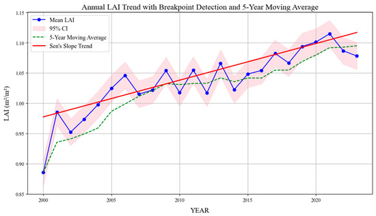
Figure 3.
Annual LAI trend with breakpoint detection and 5-year moving average.
The wavelet analysis of LAI showed that there was a significantly enhanced wavelet coefficient on a higher time scale during 2012 to 2015 (Figure 4), indicating that vegetation dynamics changed significantly on a low frequency scale during the period. This phenomenon may be driven by a combination of natural and human factors.
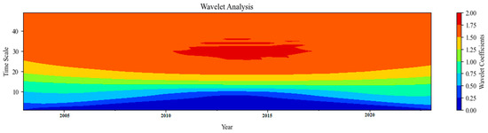
Figure 4.
Wavelet analysis of LAI time series during 2000–2023.
According to the monthly mean of the multi-year LAI during 2000–2023, vegetation in the study area showed typical unimodal annual variation (Figure 5a). Within a year, the LAI continued to rise, reaching a peak in August (about 1.68 m2/m2), and then gradually declined to the lowest value in December (about 0.64 m2/m2). This trend indicates that the vegetation in the study area had an obvious seasonal growth cycle, with a rapid growth period in spring and summer and a decline period in autumn and winter.
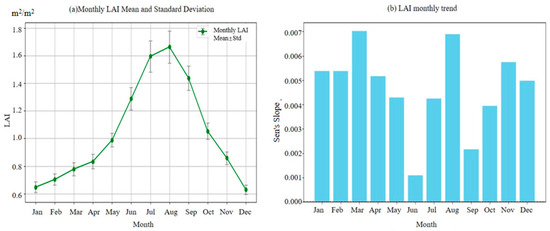
Figure 5.
Monthly mean variations in the LAI. Note: (a) monthly LAI mean and standard deviation (std); (b) LAI monthly trend.
Further analysis combined with the monthly growth slope chart shows that the change rate of the LAI in different months has obvious seasonal fluctuation characteristics (Figure 5b). The slope reached two obvious highs in spring (March) and summer (August), respectively, which indicates that the growth rate was the fastest and the vegetation growth was the most vigorous in these two periods. Although January and February were in winter, the slope remained at a medium-high level, indicating that evergreen plants or some hardy vegetation had begun to recover. The first small peak was reached in March, reflecting that most vegetation had entered the stage of rapid greening. The growth trends in April and May were relatively flat. The lowest slope in June may be related to the inhibition of vegetation growth by climate factors such as the plum rain season or high temperature and drought. The slope increased significantly again in July and reached another peak of the year in August, not as large as in March, indicating that the vegetation grew rapidly during the main growing period, which might be related to the continuous growth of late-maturing crops or certain ecosystems. The slope dropped again in September, reflecting the possibility that vegetation entered a mature or slowing growth phase. However, the slope picked up again in October and November, which may be related to the continued growth of evergreen vegetation, suitable weather conditions in autumn, or artificial planting management. Although winter starts in December, the slope remained moderately high, suggesting that vegetation in certain regions still possesses room for further growth and may also be affected by human management intervention.
In summary, the combination of the two maps (Figure 5) clearly depicts the annual change process of vegetation from germination, rapid growth, maturity to decline, which not only reflects the dynamics of vegetation under the natural climate rhythm, but also provides an important basis for further understanding of the relationship between vegetation change and climatic conditions, agricultural activities or ecological restoration measures.
3.1.2. Spatial Distribution Characteristics of LAI
As shown in Figure 6, low values of the LAI mainly existed in the upper reaches of the Jinsha River Basin, while the high values predominantly occurred in the lower reaches. This spatial heterogeneity was driven by the relatively higher temperature, increased precipitation, and stronger anthropogenic influence in the lower reaches of the Jinsha River Basin, compared with the elevated terrain, cooler conditions, and drier environment in the upstream plateau.
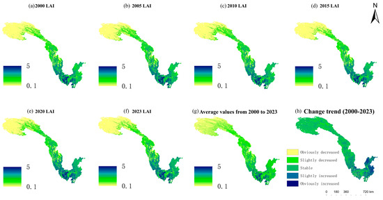
Figure 6.
Spatial distribution of LAI during 2000−2023.
Land use types in the upper, middle and lower reaches of the Jinsha River Basin are significantly different. The upper reaches of the Jinsha River Basin are mainly composed of grasslands and ice and snow areas, the middle reaches are mainly coniferous forests accompanied by grasslands and deciduous broad-leaved forests, and the lower reaches are mainly cultivated land, forest land, and impermeable water surfaces.
As a result, LAI values in the middle and lower reaches of the Jinsha River Basin were significantly higher than those in the upper reaches. From the perspective of spatial distribution, the LAI values showed the following: (1) In 2000, the 0–0.5 m2/m2 range accounted for 35.95% of the study area, forming a contiguous zone in the upper reaches of the Jinsha River Basin, with grassland and ice and snow areas as the dominant land use types. The areas with LAI values exceeding 2 m2/m2 accounted for 6.18% of the study area, predominantly distributed in the southern Jinsha River Basin. (2) In 2023, the 0–0.5 m2/m2 range accounted for 36.98% of the study area, primarily concentrated in the upper reaches of the Jinsha River Basin. The proportion of areas with LAI values exceeding 2 m2/m2 increased to 15.36%, primarily concentrated in the southern Jinsha River Basin. The rising proportion of high-LAI areas indicated gradual ecological enhancement within the Jinsha River Basin.
It was concluded from spatial autocorrelation that the LAI values in the Jinsha River Basin had a strong spatial aggregation. The Moran’s I value was 0.810420, which close to 1, indicating that the LAI values have a high positive correlation in space, that is, similar high or low values tended to cluster together rather than be randomly distributed. The Z-value of the M-K trend test was 7737.68, which indicated that the LAI data is highly unlikely to be randomly distributed but had a very obvious spatial aggregation pattern. In addition to Moran’s I, the M-K test was used to statistically assess whether the observed spatial clustering of LAI exhibited a significant monotonic pattern across the basin. This approach, though commonly applied in temporal trend analysis, has also been effectively utilized in spatial diagnostics to confirm the non-randomness of spatial distributions. Together, these methods validated the strong spatial autocorrelation of LAI values. And the p-value = 0, which indicated that the result was highly significant and almost impossible to be caused by a random distribution. These mean that the spatial aggregation of the LAI in the Jinsha River Basin was entirely driven by certain geographical, ecological or human factors, rather than being formed by chance.
Between 2000 and 2023, the LAI in the Jinsha River Basin generally exhibited an increasing trend, with the rate of increase in the southern region surpassing that in the northern region. We divided the change trend into five categories (Figure 6h), i.e., obviously decreased area (Δ ≤ −0.5 m2/m2), slightly decreased area (−0.5 m2/m2 < Δ ≤ −0.1 m2/m2), stable area (−0.1 m2/m2 < Δ ≤ 0.1 m2/m2), slightly increased area (0.1 m2/m2 <Δ ≤ 0.5 m2/m2), and obviously increased area (Δ > 0.5 m2/m2). The areas where the LAI showed an improving trend (including a slight increase and an obvious increase) accounted for 37.38% of the total area of the basin, of which 7.11% with obviously increases and 30.27% with slightly increases, indicating that the ecological conditions of nearly half of the areas in the basin were continuously improving. The increase in the LAI was mainly attributed to the transformation from grassland to forest. During the research period, the land use in the southwestern part of the Jinsha River Basin was significantly affected by urban construction and management policies, but the overall pattern was relatively stable. The relative stability of environmental and land use conditions in the southeastern region created favorable circumstances for the observed increase in the LAI. Notably, areas exhibiting stable LAI dynamics accounted for 52.44% of the total basin area, predominantly concentrated in the northern and central zones. This pattern indicated a relatively consistent land use structure and limited external disturbances in these regions. The slightly decreased area accounted for 8.82% of the total area, mainly distributed in the southern part of the basin, which may be related to local climate fluctuations or land use adjustments. Meanwhile, the significantly decreased areas accounted for only 1.36% of the total area, mainly concentrated in the central and southern parts of the basin. This change was closely related to human activities such as urban expansion and tourism development, resulting in the reduction in forest and cultivated land areas, and thereby significantly inhibited the increase of the LAI.
3.2. Analysis of Influencing Factors
Figure 7 shows the main natural and socio-economic factors influencing the LAI of the Jinsha River Basin, including topographic undulation (Elevation), slope changes (Slope), temperature distribution (TEM), precipitation patterns (Pre), land use type, and population density (Pd), etc. From the perspective of spatial distribution characteristics, the Jinsha River Basin as a whole presented a terrain pattern of being lower in the south and higher in the north, with the highest elevation reaching 6518 m. Affected by the complex terrain, the central region had a steeper slope, while the northern region had a gentler slope. In terms of temperature, the annual average temperature in the southern region was around 20 °C, while that in the northern region remained below 0 °C throughout the year. Precipitation showed a spatial distribution with higher amounts in the southern region and lower amounts in the north. In terms of land use, the north was mainly composed of glaciers and alpine meadows, while the south scattered construction land. In terms of population distribution, the population within the basin was mainly concentrated in the southern area, while human activities in the northern area were extremely scarce and almost uninhabited.
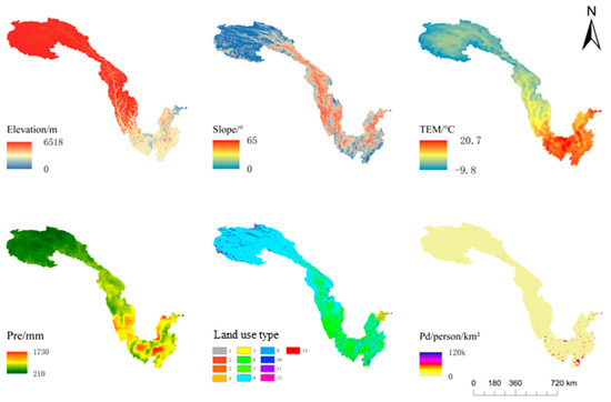
Figure 7.
Spatial distribution of the factors influencing the LAI. (Land use type: 1. cultivated land; 2. herbaceous vegetation coverage; 3. orchard; 4. evergreen broad-leaved forest; 5. deciduous broad-leaved forest; 6. coniferous forest; 7. shrub; 8. grassland; 9. impermeable water surface; 10. bare land; 11. water area; 12. wetland; 13. ice and snow area.)
Figure 8 shows the q-value of the individual factors and the interaction factors obtained by the Geodetector. The q-value is a measure of each factor’s ability to explain the target variable. A higher q-value denotes a greater explanatory influence of the factor on the target variable. With a q-value of 0.54, temperature demonstrated a notably strong influence on the LAI. The q-value of precipitation was 0.48, indicating that precipitation had a strong influence on the LAI. The q-value of elevation was 0.57, which was the highest among all individual factors, indicating that elevation had the strongest ability to explain the LAI. The interaction q-value represents the ability of the interaction between two factors to explain the target variable. The q-value of elevation and precipitation (interaction between elevation and precipitation, the same below) was 0.64, suggesting that the interplay between elevation and precipitation significantly impacted the target variable. The q-value of land use type and population density was 0.03, indicating that the interaction of these two factors had a weak explanatory power to the target variable. Elevation emerged as the most influential individual factor, indicating that elevation had the greatest influence on the LAI among all single factors. Elevation and precipitation interaction demonstrated the highest explanatory power among all interaction factors, revealing the interaction between elevation and precipitation had the greatest influence on the LAI.
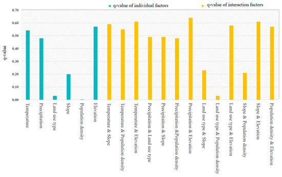
Figure 8.
Individual and interaction impacts of the LAI.
This correlation matrix heat map shows the correlation between the different variables (Figure 9). To be consistent with the Geodetector method, the reclassified LAI data was adopted in this section of the analysis. The results obtained by multiple linear regression analysis here were consistent with those obtained by Geodetector. Focus was placed on the target variable of the reclassified LAI, which had a strong positive correlation with temperature (0.66), indicating that temperature increase might promote LAI growth, while having a moderate negative correlation with elevation (−0.58). These results indicate that the LAI may be lower in higher elevations. In addition, the negative correlation between temperature and elevation was very strong (−0.83), which conformed to the geographical law, that is, the higher the elevation, the lower the temperature, but it may also cause multi-collinearity problems. In terms of land use types, there was a strong positive correlation with precipitation (0.62), suggesting that precipitation may affect the distribution of land use types. In contrast, the correlation between precipitation and the reclassified LAI was weak (0.13), which may indicate that precipitation had no obvious effect on LAI or was regulated by other factors. Hence, in the following modeling phase, temperature and elevation should be prioritized as key influencing variables.
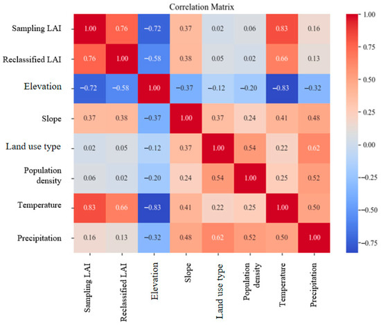
Figure 9.
Correlation matrix of the drivers influencing the LAI.
3.3. Future Prediction
Figure 10 illustrates the annual mean MODIS LAI trend from 2000 to 2023 and the forecast for the next five years (2024–2028) based on the ARIMA (1,1,0) model. According to the historical observations, the LAI exhibited a generally slow upward trend, particularly between 2000 and 2009, reflecting progressive improvements in vegetation cover. After 2010, LAI fluctuations remained within a relatively stable range (approximately 1.02 to 1.11 m2/m2), indicating ecosystem stabilization. Results of the ADF test confirmed that the time series was non-stationary. Therefore, first-order differencing was applied prior to ARIMA modeling.
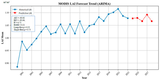
Figure 10.
Future trend prediction of the LAI in the Jinsha River Basin to 2028.
To ensure model robustness, we employed the auto ARIMA function from the R forecast package to determine the optimal (p, d, q) configuration by minimizing the AIC and BIC. ARIMA (1,1,0) model was selected, achieving the lowest AIC (−93.92) and BIC (−91.64), indicating optimal balance between model fit and parsimony. Diagnostic tests confirmed model adequacy: the Ljung–Box test showed no significant residual autocorrelation (p = 0.55), and the Jarque–Bera test indicated normally distributed residuals (p = 0.73). The AR (1) term was highly significant (p < 0.001), and no heteroscedasticity was detected (p = 0.14). In terms of predictive accuracy, the model yielded an R2 of 0.72 and RMSE of 0.21, reflecting a good fit to the observed LAI data. These evaluation metrics were included in Figure 10 to enhance the transparency and credibility of the forecasting results.
4. Discussion
This study comprehensively analyzed the spatial and temporal dynamics of the LAI in the Jinsha River Basin from 2000 to 2023, revealing a general upward trend that indicated steady improvements in vegetation cover and ecosystem health [41]. The wavelet analysis revealed pronounced LAI fluctuations during 2012–2015, suggesting the presence of low-frequency drivers. While our study did not conduct formal attribution analysis, this period coincided with the strong El Niño event of 2014–2015, which was known to cause regional temperature and precipitation anomalies [42]. These hydroclimatic shifts could have indirectly contributed to enhanced vegetation growth. Additionally, this period overlapped with ecological restoration efforts, such as reforestation and land use restructuring, as well as potential natural vegetation succession following earlier interventions. Although speculative, these overlapping events provided contextual clues that may help explain the observed LAI changes and warrant further investigation.
Spatially, the LAI presented a distinct gradient in its spatial distribution, with values decreasing from the lower to the upper reaches of the basin. The upper basin was characterized by alpine meadows and glacial regions, which were less conducive to vegetation growth due to harsh environmental conditions. In contrast, the lower basin, however, was dominated by cultivated land, forest land, and impermeable water surface, where vegetation cover was denser and more actively managed. Geodetector results further supported the dominant role of natural factors: elevation and temperature alone explained 57% and 54% of the spatial variation in the LAI, respectively, which suggested that future management strategies should be spatially differentiated and climate-adaptive. Moreover, seasonal variations in LAI trends underscored the high sensitivity of vegetation growth to climatic fluctuations—particularly changes in temperature and precipitation—highlighting the critical role of hydrothermal conditions in regulating vegetation dynamics. In addition to natural controls, socio-economic factors were playing an increasingly significant role in shaping vegetation patterns. On the positive side, ecological restoration policies and land management efforts had contributed to vegetation enhancement in many regions [43]. However, negative impacts stemming from urban expansion, deforestation, and land conversion were also evident in areas where LAI had declined [44]. These findings suggest that while environmental constraints still dominate at a macro scale, anthropogenic influences—both beneficial and detrimental—are becoming more prominent and must be integrated into future management framework. The growing interplay between human activity and environmental conditions emphasizes the need for integrated and adaptive ecological governance [45]. However, in terms of the selection of influencing factors, this study mainly focused on some typical natural and socio-economic variables and has not yet comprehensively considered other potentially important ecological and human interfering factors, such as soil type, vegetation type, ecological policies, etc.
Nevertheless, the interpretation of individual and interactive driving factors should be approached with caution due to potential multicollinearity among variables. While these variables may independently exhibit strong influence, their spatial overlap can reduce the added value of their interaction terms. Future research should consider applying multi-dimensional reduction techniques—such as Principal Component Analysis (PCA) or screening based on the Variance Inflation Factor (VIF)—to mitigate redundancy and improve interpretability [46,47].
The Geodetector model itself, while powerful for detecting spatial stratified heterogeneity and identifying driver interactions, presented several limitations. Most notably, it did not support causal inference and is highly sensitive to the classification schemes used in variable discretization. Although this study followed established reclassification strategies, the absence of confidence intervals or permutation testing for q-value limits the robustness of the results. As our goal was primarily exploratory, these limitations were deemed acceptable. However, future research should apply uncertainty quantification methods such as bootstrapping or Monte Carlo permutation tests to enhance statistical credibility.
To cross-validate the Geodetector results, a MLR model was employed to assess the relative influence of selected drivers. However, it is acknowledged that the MLR model was not used for prediction purposes, and its construction lacked formal multicollinearity diagnostics or interaction terms, which limited the reliability of coefficient estimates. Nonetheless, the MLR results were generally consistent with Geodetector findings, thereby serving as a useful supplementary validation.
In this study, land use types were incorporated as a key driver to explain the spatiotemporal variations in LAI. However, we acknowledged that the use of a single static land use map from 2020 to represent land use characteristics throughout the entire study period (2000–2023) introduced potential temporal bias [48]. Vegetation dynamics were strongly influenced by land use transitions over time, and relying on static land use type data may obscure the impact of significant land use changes, particularly in rapidly developing or ecologically restored regions. Future research can incorporate temporally explicit land use metrics, such as land use change rates, transition matrices, or dynamic land use intensity indices, to more accurately capture temporal variability and enhance the explanatory power of the driving factor.
In terms of temporal modeling, the ARIMA approach was adopted to analyze and forecast short-term LAI trends. Despite its wide application in ecological time-series modeling, ARIMA relies on assumptions of stationarity and linearity, which may not adequately capture the nonlinear and potentially non-stationary nature of vegetation dynamics under global environmental change. In this study, differencing was applied to achieve stationarity, and residual diagnostics confirmed model adequacy to a reasonable extent. However, no formal cross-validation or split-sample testing was conducted for either ARIMA or MLR, raising concerns about overfitting and limited generalizability—particularly under shifting climate and land use conditions [49]. These issues underscore the need for future studies to adopt more robust validation frameworks and consider nonlinear or hybrid models, such as machine learning-based time series models, to improve predictive accuracy.
Although this study did not partition the Jinsha River Basin into distinct ecological or climatic sub-regions, this decision was made to maintain a holistic perspective on the basin’s overall spatiotemporal dynamics. Given the pronounced gradients in elevation, temperature, and land use across the basin, the spatial heterogeneity of the LAI and its driving mechanisms could still be effectively captured using high-resolution data (250 m) and spatially explicit models such as Geodetector and spatial autocorrelation analysis. These methods allowed us to quantify dominant influencing factors and their interactions without the need for a priori zoning, ensuring comparability across the study area.
In summary, the following four directions are the research directions for the future. Firstly, from the perspective of influencing factors, more ecological environmental variables and human activity indicators should be introduced to construct a multi-dimensional driving factor system so as to improve the scientificity and comprehensiveness of the analysis of LAI change mechanisms [38]. Secondly, in terms of model construction and prediction, information such as climate model output, socio-economic scenarios, and land use change simulations should be incorporated to support scenario-based analysis of future vegetation trends. Thirdly, advances in remote sensing technology and data fusion offer new opportunities for enhancing LAI estimation. Specifically, the integration of multi-source remote sensing products with high-resolution temporal reconstruction can significantly improve the spatial and temporal accuracy of LAI datasets, providing stronger support for long-term ecological monitoring and river basin-scale management. Fourthly, more robust statistical analyses should be conducted to improve inference reliability and model transparency. As discussed above, approaches such as multicollinearity diagnostics (e.g., VIF), uncertainty quantification (e.g., bootstrapping, permutation tests), and dimensionality reduction techniques (e.g., PCA) are critical for reducing redundancy and enhancing interpretability. Finally, sub-regional analyses should be further explored to account for the pronounced ecological and climatic heterogeneity within the basin. Dividing the study area into stratified zones (e.g., high-altitude vs. low-altitude regions, or ecological function zones) would allow for more targeted investigation of spatially heterogeneous drivers and could yield insights more relevant to localized land management and policy formulation.
5. Conclusions
As a critical ecological barrier in southwest China, the Jinsha River Basin is vital for safeguarding regional ecological stability and biodiversity. By integrating MODIS LAI products with meteorological and socio-economic data, this study has conducted a comprehensive analysis of the spatiotemporal variation and driving forces of the LAI from 2000 to 2023. The findings offer valuable insights to support ecological conservation, land use optimization, and sustainable development planning in mountainous river basins.
The main conclusions are as follows: (1) During 2000–2023, the LAI in the Jinsha River Basin has shown a stable growth trend with seasonal differences, indicating that the ecological conditions have been gradually improving. (2) The LAI exhibits a clear spatial gradient, characterized by lower levels in the upper basin and higher levels in the lower basin. This distribution was primarily influenced by variations in elevation and temperature. (3) The results of Geodetector further supported the significant role of elevation and temperature, explaining 57% and 54% of the spatial variations of the LAI, respectively. These findings emphasized the dominant role of natural environmental factors in influencing vegetation distribution at the regional scale. However, socio-economic activities were also playing an increasingly important role. Active human intervention, such as ecological restoration policies, can help improve the LAI, while the adverse effects of urban expansion and land use change may lead to vegetation degradation. (4) The future LAI trend during 2024–2028 appeared stable without significant changes. These results offer a scientific foundation for regional ecological conservation and land use planning and offer important insights into vegetation changes under the dual pressures of climate change and human activities.
Based on a comprehensive understanding of the spatiotemporal evolution of the LAI and its dominant natural and anthropogenic drivers, this study proposes five targeted policy recommendations to support ecological management, land use planning, and sustainable development in mountainous river basins such as the Jinsha River Basin. Firstly, ecological restoration should be prioritized in areas where the LAI has shown a persistent LAI decline, especially in ecologically fragile zones in the upper basin. These efforts should be guided by spatially explicit, long-term monitoring data to enhance restoration effectiveness and resource allocation precision. Secondly, land use planning should integrate topographic and climatic zoning principles. Elevation and temperature, as the most influential environmental variables identified in this study, should be embedded into regional planning frameworks to ensure that land management strategies are adapted to environmental gradients. Thirdly, it is necessary to balance urban development and ecological protection through integrated land use strategies. This includes restricting high-intensity land conversion in ecologically sensitive areas and enhancing landscape connectivity to maintain biodiversity and ecological function. Fourthly, the transformation of socio-economic activities towards sustainability should be promoted. Efforts should focus on developing eco-friendly agricultural practices, advancing ecological infrastructure, and adopting low-impact urban design to mitigate anthropogenic pressures on vegetation systems. Fifthly, remote sensing and big data infrastructure should be further enhanced to support high-resolution, long-term ecological monitoring. Such improvements will facilitate evidence-based and adaptive decision-making, particularly in complex mountain ecosystems vulnerable to both climate change and human disturbances. By translating empirical results into actionable strategies, this study contributes valuable scientific support for integrated land governance, ecosystem restoration, and the realization of climate-resilient, sustainable development goals in the Jinsha River Basin and help achieve ecosystem resilience, sustainable territorial development, and improved ecological service provision under the dual pressures of climate change and anthropogenic influence.
Author Contributions
Conceptualization, R.Z., J.L., and Y.B.; methodology, J.Y. and J.T.; software, J.Y. and Z.L.; validation, Z.X., X.C., and Y.B.; formal analysis, Z.X., J.T., and Z.L.; investigation, J.L., L.X., and X.C.; resources, R.Z. and J.L.; data curation, R.Z., Z.X., and L.X.; writing—original draft preparation, R.Z., J.T., and J.Y.; writing—review and editing, J.L., X.C., J.Y., and Y.B.; visualization, J.Y., L.X., and Z.L.; supervision, Y.B.; project administration, R.Z., X.C., Y.B., and Z.L.; funding acquisition, J.L., Y.B., R.Z., and Z.L. All authors have read and agreed to the published version of the manuscript.
Funding
This work was supported by China Yangtze Power Co., Ltd., Three Gorges Jinsha River Yunchuan Hydropower Development Co., Ltd. (Contract No. Z542302008), the National Natural Science Foundation of China (No. 42201050), and the Hubei Provincial Natural Science Foundation of China (No. 2022CFB836).
Data Availability Statement
The original contributions presented in this study are included in this article. Further inquiries can be directed to the corresponding author.
Conflicts of Interest
The authors declare no conflicts of interest.
References
- Zhang, L.; Hu, X.; Cherubini, F. Accounting for exact vegetation index recording date to enhance evaluation of time-lagged and accumulated climatic effects on global vegetation greenness. Environ. Res. 2025, 275, 121398. [Google Scholar] [CrossRef]
- Shi, W.; Lu, P.; Yang, H.; Han, J.; Wang, Q. Quantifying the relative importance of natural and human factors on vegetation dynamics in China’s western frontiers during 2010–2021. Environ. Res. 2025, 271, 121120. [Google Scholar] [CrossRef]
- Zhang, Z.; Xin, Q.; Li, W. Machine learning-based modeling of vegetation leaf area index and gross primary productivity across North America and comparison with a process-based model. J. Adv. Model. Earth Syst. 2021, 13, e2021MS002802. [Google Scholar] [CrossRef]
- Chen, J.M.; Black, T.A.; Adams, R.S. Evaluation of hemispherical photography for determining plant area index and geometry of a forest stand. Agric. For. Meteorol. 1991, 56, 129–143. [Google Scholar] [CrossRef]
- Fang, H.; Baret, F.; Plummer, S.; Schaepman-Strub, G. An overview of global leaf area index (LAI): Methods, products, validation, and applications. Rev. Geophys. 2019, 57, 739–799. [Google Scholar] [CrossRef]
- Wei, B.; Ma, X.; Guan, H.; Yu, M.; Yang, C.; He, H.; Wang, F.; Shen, P. Dynamic simulation of leaf area index for the soybean canopy based on 3D reconstruction. Ecol. Inform. 2023, 75, 102070. [Google Scholar] [CrossRef]
- Hashimoto, H.; Wang, W.; Milesi, C.; White, M.A.; Ganguly, S.; Gamo, M.; Hirata, R.; Myneni, R.B.; Nemani, R.R. Exploring Simple Algorithms for Estimating Gross Primary Production in Forested Areas from Satellite Data. Remote Sens. 2012, 4, 303–326. [Google Scholar] [CrossRef]
- Leuning, R.; Zhang, Y.Q.; Rajaud, A.; Cleugh, H.; Tu, K. A simple surface conductance model to estimate regional evaporation using MODIS leaf area index and the Penman-Monteith equation. Water Resour. Res. 2008, 406, W10419. [Google Scholar] [CrossRef]
- Ahlström, A.; Xia, J.; Arneth, A.; Luo, Y.; Smith, B. Importance of vegetation dynamics for future terrestrial carbon cycling. Environ. Res. Lett. 2015, 10, 054019. [Google Scholar] [CrossRef]
- Sun, Y.; Qin, Q.; Zhang, Y.; Ren, H.; Han, G.; Zhang, Z.; Zhang, T.; Wang, B. A leaf chlorophyll vegetation index with reduced LAI effect based on Sentinel-2 multispectral red-edge information. Comput. Electron. Agric. 2025, 236, 110500. [Google Scholar] [CrossRef]
- Zhuang, Z.-H.; Tsai, H.P.; Chen, C.-I.; Yang, M.-D. Subtropical region tea tree LAI estimation integrating vegetation indices and texture features derived from UAV multispectral images. Smart Agric. Technol. 2024, 9, 100650. [Google Scholar] [CrossRef]
- Piao, S.; Yin, G.; Tan, J.; Cheng, L.; Huang, M.; Li, Y.; Liu, R.; Mao, J.; Myneni, R.B.; Peng, S.; et al. Detection and attribution of vegetation greening trend in China over the last 30 years. Glob. Change Biol. 2015, 21, 1601–1609. [Google Scholar] [CrossRef] [PubMed]
- Tesemma, Z.K.; Wei, Y.; Western, A.W.; Peel, M.C. Leaf area index variation for crop, pasture, and tree in response to climatic variation in the Goulburn–Broken catchment, Australia. J. Hydrometeorol. 2014, 15, 1592–1606. [Google Scholar] [CrossRef]
- Sun, K.; Zeng, X.; Li, F. Study on the dominant climatic driver affecting the changes of LAI of ecological fragile zones in China. J. Nat. Resour. 2021, 36, 1873–1892. [Google Scholar] [CrossRef]
- Huang, A.; Shen, R.; Shi, C.; Sun, S. Effects of satellite LAI data on modelling land surface temperature and related energy budget in the Noah-MP land surface model. J. Hydrol. 2022, 613, 128351. [Google Scholar] [CrossRef]
- Yao, L.; Wang, X.; Zhang, J.; Yao, F. Analysis of spatiotemporal variation and driving forces of leaf area index in Hainan Island over the last 20 years based on MODIS data. Chin. J. Eco-Agric. 2024, 32, 1719–1730. [Google Scholar]
- Zou, Y.; Chen, W.; Li, S.; Wang, T.; Yu, L.; Xu, M.; Singh, R.P.; Liu, C.-Q. Spatiotemporal Changes in Vegetation in the Last Two Decades (2001–2020) in the Beijing–Tianjin–Hebei Region. Remote Sens. 2022, 14, 3958. [Google Scholar] [CrossRef]
- Reygadas, Y.; Jensen, J.L.R.; Moisen, G.G.; Currit, N.; Chow, E.T. Assessing the relationship between vegetation greenness and surface temperature through Granger causality and Impulse-Response coefficients: A case study in Mexico. Int. J. Remote Sens. 2020, 41, 3761–3783. [Google Scholar] [CrossRef]
- Liang, S.; Yi, Q.; Liu, J. Vegetation dynamics and responses to recent climate change in Xinjiang using leaf area index as an indicator. Ecol. Indic. 2015, 58, 64–76. [Google Scholar] [CrossRef]
- Ning, L.; Peng, W.; Yu, Y.; Xiang, J.; Wang, Y. Quantifying vegetation change and driving mechanism analysis in Sichuan from 2000 to 2020. Front. Environ. Sci. 2023, 11, 1261295. [Google Scholar] [CrossRef]
- Chen, Y.; Zhao, Q.; Liu, Y.; Zeng, H. Exploring the impact of natural and human activities on vegetation changes: An integrated analysis framework based on trend analysis and machine learning. J. Environ. Manag. 2025, 374, 124092. [Google Scholar] [CrossRef] [PubMed]
- Bai, Y.; Liu, M.; Guo, Q.; Wu, G.; Wang, W.; Li, S. Diverse responses of gross primary production and leaf area index to drought on the Mongolian Plateau. Sci. Total Environ. 2023, 902, 166507. [Google Scholar] [CrossRef] [PubMed]
- Chen, B.; Li, X.; Xiao, X.; Zhao, B.; Dong, J.; Kou, W.; Qin, Y.; Yang, C.; Wu, Z.; Sun, R.; et al. Mapping tropical forests and deciduous rubber plantations in Hainan Island, China by integrating PALSAR 25-m and multi-temporal Landsat images. Int. J. Appl. Earth Obs. Geoinf. 2016, 50, 117–130. [Google Scholar] [CrossRef]
- Guo, Y.; Cheng, L.; Ding, A.; Yuan, Y.; Li, Z.; Hou, Y.; Ren, L.; Zhang, S. Geodetector model-based quantitative analysis of vegetation change characteristics and driving forces: A case study in the Yongding River basin in China. Int. J. Appl. Earth Obs. Geoinf. 2024, 132, 104027. [Google Scholar] [CrossRef]
- Guo, D.; Song, X.; Hu, R.; Ma, R.; Zhang, Y.; Gao, L.; Zhu, X.; Kardol, P. Spatio-temporal variation in leaf area index in the Yan Mountains over the past 40 years and its relationship to hydrothermal conditions. Ecol. Indic. 2023, 157, 111291. [Google Scholar] [CrossRef]
- Pennino, M.G.; Bellido, J.M.; Conesa, D.; Coll, M.; Tortosa-Ausina, E. The analysis of convergence in ecological indicators: An application to the Mediterranean fisheries. Ecol. Indic. 2017, 78, 449–457. [Google Scholar] [CrossRef]
- Stokes, E.C.; Seto, K.C. Characterizing urban infrastructural transitions for the Sustainable Development Goals using multi-temporal land, population, and nighttime light data. Remote Sens. Environ. 2019, 234, 111430. [Google Scholar] [CrossRef]
- Li, C.; Jin, Z.; Gou, L.F.; Xu, Y.; Deng, L. Hydrological regulation of seasonal Mg isotopic variation in the upper Jinsha River draining the eastern Tibetan Plateau. Chem. Geol. 2025, 684, 122773. [Google Scholar] [CrossRef]
- Zhang, Z.F.; Liu, S.Y.; Ma, K.; Zhang, X.; Yang, Y.; Cui, F. Runoff simulation of the upper Jinsha River Basin based on LSTM driven by elevation dependent climatic forcing. Prog. Geogr. 2023, 42, 1139–1152. [Google Scholar] [CrossRef]
- An, N.; Zhang, H.; Xu, Y.; Liu, H.; Sun, J. Spatiotemporal evolution characteristics of meteorological and agricultural droughts in Jinsha River Basin. Res. Soil Water Conserv. 2025, 32, 176–188. [Google Scholar]
- Lv, H.; Gao, Z.; Yan, D.; Shang, W.; Zheng, X. Ecological flow research in response to hydrological variation: A case study of the Jinsha River Basin, China. Desalination Water Treat. 2024, 320, 100777. [Google Scholar] [CrossRef]
- Gao, F.; Pan, J.; Gong, Z. Detection of spatial and temporal variation characteristics of vegetation cover in the Lower Mekong region and the influencing factors. Sci. Rep. 2024, 14, 26673. [Google Scholar] [CrossRef]
- Mann, H.B. Nonparametric tests against trend. Econom. J. Econom. Soc. 1945, 13, 245–259. [Google Scholar] [CrossRef]
- Cheruiyot, K. Detecting spatial economic clusters using kernel density and global and local Moran’s I analysis in Ekurhuleni metropolitan municipality, South Africa. Reg. Sci. Policy Pract. 2022, 14, 307–328. [Google Scholar] [CrossRef]
- Lu, Y.; Yang, X.; Bian, D.; Chen, Y.; Li, Y.; Yuan, Z.; Wang, K. A novel approach for quantifying water resource spatial equilibrium based on the regional evaluation, spatiotemporal heterogeneity and geodetector analysis integrated model. J. Clean. Prod. 2023, 424, 138791. [Google Scholar] [CrossRef]
- Wang, Z.; Li, X.; Zhao, H. Identifying spatial influence of urban elements on road-deposited sediment and the associated phosphorus by coupling Geodetector and Bayesian Networks. J. Environ. Manag. 2022, 315, 115170. [Google Scholar] [CrossRef]
- Siddique, M.A.B.; Mahalder, B.; Haque, M.M.; Ahammad, A.K.S. Forecasting air temperature and rainfall in Mymensingh, Bangladesh with ARIMA: Implications for aquaculture management. Egypt. J. Aquat. Res. 2025, 1687–4285. [Google Scholar] [CrossRef]
- Juraphanthong, W.; Kesorn, K. Autoregressive integrated moving average with semantic information: An efficient technique for intelligent prediction of dengue cases. Eng. Appl. Artif. Intell. 2025, 143, 109985. [Google Scholar] [CrossRef]
- Wang, X.; Kang, Y.; Hyndman, R.J.; Li, F. Distributed ARIMA models for ultra-long time series. Int. J. Forecast. 2023, 39, 1163–1184. [Google Scholar] [CrossRef]
- Lu, J.; Li, J.; Fu, H.; Zou, W.; Kang, J.; Yu, H.; Lin, X. Estimation of rice yield using multi-source remote sensing data combined with crop growth model and deep learning algorithm. Agric. For. Meteorol. 2025, 370, 110600. [Google Scholar] [CrossRef]
- Liu, X.; Zhao, W.; Yao, Y.; Pereira, P. The rising human footprint in the Tibetan Plateau threatens the effectiveness of ecological restoration on vegetation growth. J. Environ. Manag. 2024, 351, 119963. [Google Scholar] [CrossRef] [PubMed]
- Nizamani, M.M.; Hughes, A.C.; Wang, Y.; Zhang, H.L.; Lai, Z. Climate extremes and socioeconomic impact of El Niño and La Niña events. Environ. Dev. 2025, 56, 101276. [Google Scholar] [CrossRef]
- Tian, Z.; Wang, C.; Wang, T.; Liu, Z.; Ding, L.; Mao, X. Natural and anthropogenic influences on short-term forest growth status: Evidence and mechanisms from China. J. Environ. Manag. 2025, 389, 126084. [Google Scholar] [CrossRef]
- Wang, C.; Wang, Q.; Liu, N.; Sun, Y.; Guo, H.; Song, X. The impact of LUCC on the spatial pattern of ecological network during urbanization: A case study of Jinan City. Ecol. Indic. 2023, 155, 111004. [Google Scholar] [CrossRef]
- Gong, D.; Huang, M.; Ge, Y.; Zhu, D.; Chen, J.; Chen, Y.; Zhang, L.; Hu, B.; Lai, S.; Lin, H. Revolutionizing ecological security pattern with multi-source data and deep learning: An adaptive generation approach. Ecol. Indic. 2025, 173, 113315. [Google Scholar] [CrossRef]
- Mohammadreza, B.; Behnood, H.R.; Forward, S.; Andersson, J. A tree-based extended model to predict intention to speed for taxi drivers. Transp. Res. Part F Traffic Psychol. Behav. 2024, 103, 190–200. [Google Scholar]
- Zeng, W.; Wan, X.; Lei, M.; Gu, G.; Chen, T. Influencing factors and prediction of arsenic concentration in Pteris vittata: A combination of geodetector and empirical models. Environ. Pollut. 2022, 292, 118240. [Google Scholar] [CrossRef]
- Mazy, F.-R.; Longaretti, P.-Y. Towards a generic theoretical framework for pattern-based LUCC modeling: An accurate and powerful calibration–estimation method based on kernel density estimation. Environ. Model. Softw. 2022, 158, 105551. [Google Scholar] [CrossRef]
- Jiang, B.; Zhang, C.; Liu, Z.; Wen, J.; Zhu, J.; Xu, L.; Wang, F. Tailoring an economic-ecological-tourism coupling framework for arid-region ski resorts: A PSR model-based case study of Xinjiang, China. Ecol. Indic. 2025, 178, 113881. [Google Scholar] [CrossRef]
Disclaimer/Publisher’s Note: The statements, opinions and data contained in all publications are solely those of the individual author(s) and contributor(s) and not of MDPI and/or the editor(s). MDPI and/or the editor(s) disclaim responsibility for any injury to people or property resulting from any ideas, methods, instructions or products referred to in the content. |
© 2025 by the authors. Licensee MDPI, Basel, Switzerland. This article is an open access article distributed under the terms and conditions of the Creative Commons Attribution (CC BY) license (https://creativecommons.org/licenses/by/4.0/).